IB-UQ: Information bottleneck based uncertainty quantification for neural function regression and neural operator learning
Abstract
We propose a novel framework for uncertainty quantification via information bottleneck (IB-UQ) for scientific machine learning tasks, including deep neural network (DNN) regression and neural operator learning (DeepONet). Specifically, we incorporate the bottleneck by a confidence-aware encoder, which encodes inputs into latent representations according to the confidence of the input data belonging to the region where training data is located, and utilize a Gaussian decoder to predict means and variances of outputs conditional on representation variables. Furthermore, we propose a data augmentation based information bottleneck objective which can enhance the quantification quality of the extrapolation uncertainty, and the encoder and decoder can be both trained by minimizing a tractable variational bound of the objective. In comparison to uncertainty quantification (UQ) methods for scientific learning tasks that rely on Bayesian neural networks with Hamiltonian Monte Carlo posterior estimators, the model we propose is computationally efficient, particularly when dealing with large-scale data sets. The effectiveness of the IB-UQ model has been demonstrated through several representative examples, such as regression for discontinuous functions, real-world data set regression, learning nonlinear operators for partial differential equations, and a large-scale climate model. The experimental results indicate that the IB-UQ model can handle noisy data, generate robust predictions, and provide confident uncertainty evaluation for out-of-distribution data.
Keywords:
Information bottleneck , Uncertainty quantification, Deep neural networks , Operator learning , DeepONetMain text
Scientific machine learning, particularly physics-informed deep learning, has achieved significant success in modelling and predicting the response of complex physical systems Karniadakis et al. 2021, Willard et al. 2022. Deep neural networks (DNNs), which possess the universal approximation property for continuous functions Chen and Chen 1993, has been widely employed in approximating the solutions of forward and inverse ordinary/partial differential equations Lagaris et al. 1998, Khoo et al. 2021, Raissi et al. 2017, Liao and Ming 2021, Guo et al. 2022a, Guo et al. 2022b, Huang et al. 2022, Gao et al. 2022. They have also been proven useful in solving high-dimensional partial differential equations E and Yu 2018, Zang et al. 2020 and discovering equations from data Brunton et al. 2016, Long et al. ????. Another prominent direction in scientific machine learning lie in learning continuous operators or complex systems from streams of scattered data. One representitave approach is the deep operator network (DeepONet) proposed by Lu et al. Lu et al. 2021. DeepONet’s original structure is based on the universal approximation theorem of nonlinear operators Chen and Chen 1995 and has been successfully used in multiscale and multiphysics problems Lin et al. 2021, Mao et al. 2021. To further enhance the performance of DeepONet, a physics-informed architecture was proposed in Wang et al. 2021. Another structure for operator learning is the Fourier Neural Operator Li et al. 2020, which parameterizes the integral kernel in Fourier space. Recently, a novel kernel-coupled attention operator learning method was developed in Kissas et al. 2022 inspired by the attention mechanism’s success in deep learning.
There are several sources of uncertainty that can arise when using DNNs in scientific machine learning tasks, including noisy and limited data, neural network parameters, unknown parameters, and incomplete physical models, among others Psaros et al. 2022. Thus it is crucial to accurately quantify and predict uncertainty for deep learning to be reliably used in practical applications. Proper uncertainty estimates are essential to evaluate a model’s confidence in its predictions. The most popular approach of uncertainty quantification (UQ) in the deep learning community is based on the Bayesian framework MacKay 1995, Neal 2012, Gal and Ghahramani ????, where the uncertainty is obtained by performing posterior inference using Bayes’ rule given observational data and prior beliefs. Alternative UQ methods are based on ensembles of DNN optimization iterates or independently trained DNNs Lakshminarayanan et al. 2017, Malinin and Gales 2018, Fort et al. 2019, as well as on the evidential framework Sensoy et al. 2018, Amini et al. 2020. Uncertainty quantification (UQ) in the context of scientific machine learning is a more challenging task due to the inclusion of physical models. There have been few works on UQ for scientific machine learning especially for operator learning till now. Psaros et al. provided an extensive review and proposed novel methods of UQ for scientific machine learning in Psaros et al. 2022, accompanied by an open-source Python library termed NeuralUQ Zou et al. 2022. Other related UQ research for operator learning and reliable DeepONet method can be found in Moya et al. 2023, Lin et al. 2021, Yang et al. 2022, Zhu et al. 2022.
The information bottleneck (IB) principle was initially introduced by Tishby et al. in their work Tishby 1999. The principle seeks to find an encoding that can maximally express the target variable while being maximally compressive about the input . To achieve this, the principle proposes maximizing the objective function , where is the Lagrange multiplier. The theoretical framework of the IB principle is used to analyze deep neural networks in Tishby and Zaslavsky ????. A variational approximation of IB (VIB) was then established in Alemi et al. 2016, where a nerual network is used to parameterise the information bottleneck model. Further results in Alemi et al. 2018 show VIB incorporates uncertainty naturally thus can improve calibration and detect out-of-distribution data. Addational related research including different approximation approaches for the IB objective, the connection between IB and the stochastic gradient descent training dynamics can be found in Kolchinsky et al. 2019, Shwartz-Ziv and Tishby 2017, Saxe et al. 2019 and references therein. While many existing studies on IB-based uncertainty quantification have focused on classification tasks, there has been limited attention given to regression tasks thus far.

In this paper, we put effort into establishing a novel framework for uncertainty quantification via information bottleneck (IB-UQ) in scientific machine learning tasks, including deep neural network regression and DeepONet operator learning. A schematic of IB-UQ method for function regression is shown in Figure 1, which is specifically designed to improve uncertainty prediction for both in-distribution and out-of-distribution inputs. To achieve this, we employ the general incompressible-flow network (GIN) to generate augmented data from a "wide" distribution, that has a high entropy and can cover the domain of the training data, and establish a data augmentation based IB objective. Additionally, we introduce a confidence-aware encoder that maps the input to a latent representation that can be used to predict the mean and covariance of the output, allowing for more accurate and reliable uncertainty estimates. To ensure that our model can be trained efficiently, we construct a tractable variational bound on the IB objective using a normalizing flow reparameterization, which enables all parameters of the model to be trained according to the bound. The main contributions of this work can be summarized as follows:
- 1.
We introduce a novel framework for quantifying uncertainty in scientific machine learning tasks, including deep neural network (DNN) regression and neural operator learning (DeepONet).
- 2.
The proposed IB-UQ method can obtain both mean and uncertainty estimates of the prediction via explicitly modeling the random representation variables. In comparison to the existing gold standard UQ method, such as Bayesian Neural Network with Hamiltonian Monte Carlo posterior estimation Psaros et al. 2022, the proposed new model is both easy to implement and efficient for large-scale data problems.
- 3.
The proposed model is capable of providing confident uncertainty evaluation for out-of-distribution data, which is crucial for the use of neural network-based methods in risk-related tasks and applications. This capability enhances the model’s reliability and applicability in real-world scenarios where the presence of such data is inevitable.
Results
We demonstrate the effectiveness of our proposed IB-UQ method on various deep neural network (DNN) function regression and deep operator learning problems. We will present detailed experimental results for several benchmark problems, including regression of a discontinuous function, operator learning for two partial differential equations, California housing prices regression, and a large-scale climate modeling task. Additionally, we report more experimental analysis and comparison results for the discontinuous function regression problem and climate modeling in S7 Additional results. The hyperparameters and neural network architectures we used in these examples are summarized in Supplementary Information S8 Hyperparameters and neural network architectures used in the numerical examples.
The numerical results indicate the IB-UQ model’s ability to provide robust functional predictions, while also demonstrate its ability to handle noisy data and provide confident uncertainty estimates for out-of-distribution samples.
The codes used to generate the results will be released in GitHub upon publication of the paper.
Discontinuous function regression
We first consider a one-dimensional discontinuous test function
| (1) |
The training dataset consists of , unless otherwise specified, equidistant measurements of at . The data is contaminated with zero-mean Gaussian noise .
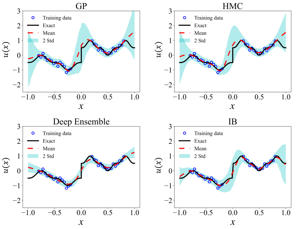
We use the IB-UQ algorithm to predict the values of at any unseen position with uncertainty estimates with , and compare IB-UQ method with three efficient UQ methods for scientific machine learning problems given in Psaros et al. 2022, including Gaussian processes regression (GP), Bayesian Neural networks with Hamiltonian Monte Carlo posterior sampling method (HMC), and Deep Ensemble method. Figure 2 presents the mean prediction and uncertainty estimates, i.e. the standard deviations, obtained by the four UQ methods. We can see that (1) all the four methods provide good mean prediction compared with the exact solution; (2) similar as GP and HMC methods, IB-UQ method can also provide larger standard deviations (i.e., uncertainty) at the regions with fewer training data, i.e., , which is important in risk-sensitive applications, where computational methods should be able to distinguish between interpolation domain and extrapolation domain. However, the uncertainty of the Deep Ensemble method does not increase obviously for the out-of-distribution (OOD) test data. Although GP and HMC are often considered the gold standard for Bayesian neural network (BNN) methods, they both have limitations. Gaussian processes regression, for instance, is hard to cope with nonlinearities when applied to solve partial differential equations (PDEs). Additionally, the HMC method can be computationally expensive, particularly for large data sets, compared to our IB-UQ method, which does not require posterior distribution sampling and is easy to implement.
Diffusion-reaction equation
Here we consider the following diffusion-reaction equation
| (2) |
with zero initial and boundary conditions Zhu et al. 2022. Here denotes the diffusion coefficient and the reaction rate. In this example, is set at and is set at . We aim to use our information bottleneck based UQ method to learn the operator that maps the source term to the solution of the system (2) with :
The training and testing data are generated as follows. The input functions are sampled from a mean-zero Gaussian random process with an squared-exponential kernel
where represents the correlation length. The training dataset uses and each realization of is recorded on an equi-spaced grid of sensor locations. Then we solve the diffusion-reaction system using a second-order implicit finite-difference method on a grid to obtain the training data of .
We totally generate input/output function pairs for training the IB-UQ model. To report the performance of the IB-UQ model for out-of-distribution data detection, the test data are obtained from Gaussian process with different correlation length scales. Specifically, for in-distribution (ID) test data, corresponds to a sample from the same stochastic process as used for training, i.e . For out-of-distribution (OOD) test data, corresponds to a sample from a stochastic process with different correlation length of the training data, i.e. or . We consider the scenario that both the training/test data values are contaminated with Gaussian noise with standard deviation equal to . The regularization parameter in IB-UQ objective function (6) for operator learning is set to .

The root mean square error (RMSE) between the ground truth solution and the IB-UQ DeepONet predictive mean as well as the uncertainty estimate are reported in Figure 3. We can see that when the training and test functions are sampled from the same space (), i.e. ID test data, the error is smaller. However, the RMSE of IB-UQ model increases significantly for OOD data with . Nevertheless, for OOD data with , IB-UQ DeepONet still has a small error. Potential explanation is with a larger leading to smoother kernel functions and DeepONet structure can predict accurately for smoother functions. These results are consistent with the observations reported in Lu et al. 2021, Yang et al. 2022. Figure 4 presents comparison between the ground truth solution and the IB-UQ predictive mean and uncertainty tested on data generated with different correlation length. We obsever that the computational absolute errors between the predicted means and the reference solutions are bounded by the predicted uncertainties, 2 standard deviation, for the the three different cases. Moreover, despite the predictions of the IB-UQ not being accurate on testing data with smaller , the larger uncertainty obtained from IB-UQ reflects the inaccuracy of the predictions. Thus IB-UQ model can provide reliable uncertainty estimates for OOD data.


Advection equation
We now consider to train the IB-UQ model to learn the operator that maps to the solution :
defined by the following advection equation Zhu et al. 2022
| (3) |
with the initial conditional and boundary conditioal . We take in form of to guarantee .


The training data set is constructed by sampling from a Gaussian random field with an squared exponential kernel with correlation length , and then use them as inputs to solve the advection equation via a finite difference method to obtain input and output function pairs, where the measurements on grid points of each are available. To test the performance of the IB-UQ method on ID and OOD data, we generate three test datasets of 1000 functions with respectively. We consider the scenario that both training/test data values are contaminated with Gaussian noise with standard deviation equal to 0.01.
We present the comparison between the ground truth solution and the IB-UQ predictive mean and uncertainty in Figure 5 for testing cases with different correlation length . We also plot 4 time-snapshots from 1 out of 1000 randomly choosing testing samples. We can see that the absolute errors between the predicted means and the reference solutions are bounded by the predicted uncertainties. We also observe that for OOD test sample generated with correlation length , the prediction mean is less accurate than those of ID and OOD test sample with larger correlation length . Thus larger uncertainty is obtained in the cases where the predictive mean is not accurate. This example also demonstrate that the IB-UQ model can provide resonable predictions with confident uncertainty estimates on noisy unseen dataset.
California housing prices data set
To further evaluate the performance of the proposed IB-UQ method on real data set applications, we next consider the California housing prices regression problem with data set distributed via the scikit-learn package Pedregosa et al. 2011, which was originally published in Pace and Barry 1997. The data set consists of 20640 total samples and 8 features including median household income, median age of housing use, average number of rooms, etc. To obtain the ID and OOD data set, we employ the local outlier factor method (LOF) Breunig et al. ???? to divide the whole data set into four blocks based on three local outlier factor, i.e. -2, -1.5 and -1.2, as shown in the schematic diagram Figure 6(a). We regard the corresponding data with LOF score larger than -1.2 as in-distribution data(ID), including 18,090 samples. Data with LOF score smaller than -1.2 is recorded as the OOD data, which is divided into three parts according to the LOF score. Specifically, OOD part1 contains 2192 samples satisfying -1.5<score<-1.2, OOD part2 contains 305 samples satisfying -2<score<-1.5, OOD part3 contains 53 samples satisfying, respectively. We randomly choose of the ID data set for training and the rest samples are used for testing.
The absolute error of the predict mean and uncertainty estimates for both ID test data and OOD test data are reported in Figure 6(b)-(c). We can see from the plots that the absolute error of ID data mean prediction is smaller than those of OOD test data. Further, The absolute error increases significantly for OOD data with decreasing LOF and the uncertainty covers the absolute error of the mean for both ID and OOD data.
Climate Model
Finally, we consider a large-scale climate modeling task, which aims to learn an operator that maps the surface air temperature field over the Earth to the surface air pressure field given real historical weather station data Yang et al. 2022. This mapping takes the form
| (4) |
with represent the temperature and pressure respectively and correspond to latitude and longitude coordinates pairs to specify the location on the surface of the earth.


The training and testing data sets are obtained according to the data sets used in Yang et al. 2022. The training data set is generated by taking measurements from daily data of surface air temperature and pressure from 2000 to 2005. Concretely, input/output function pairs are obtained on a mesh with grid. We randomly select points during the training stage. The testing data is measured in the same way and contains input/output function pairs on a mesh with grid. For the details of the data generation, please see the github code accompanying reference Yang et al. 2022.
To enhance the performance of IB-UQ DeepONet for this example, we use following Harmonic Feature Expansion established in Lu et al. 2022
| (5) |
as the input of the trunk network (see Eqs. (11, 14)), where is the order of the harmonic basis and we set it equal to 5 in our simulation. Meanwhile, to demonstrate that the IB-UQ method can detect OOD data, we consider three cases in our training process: 1) Case 1 uses full training data set with sample pairs; 2) Case 2 uses training data after removing the data of the second quarter of each year. The training data set has sample pairs; 3) Case 3 uses data after removing all data from the second and third quarter of each year. The training data set for this case has sample pairs. In Figure 7, we show the exact pressure field, the predictive mean pressure field, and representative predictions for the three different cases. We observe that the model obtain larger error and uncertainty for the prediction of the unseen data. While for the in distribution data, the model can provide more accurate mean prediction and reasonable uncertainty estimates, which means the uncertainty bound can cover the absolute error.
Methods
IB-UQ for DNN function regression
Our proposed approach, termed IB-UQ, utilizes the information bottleneck method for function regression and provides scalable uncertainty estimation in function learning. In this section, we will describe the theory of the method and the architecture of the model in detail.
Formulation: Assume and is a function defined on , i.e. . Given a set of paired noisy observations , where , . Our goal is to construct a deep learning model that can predict the value of at any new location as well as provide reliable uncertainty estimation. Following the main idea of information bottleneck developed by Tishby et al. Tishby and Zaslavsky ????, we encode the input to a latent representation by enforcing the extraction of essential information relevant to the prediction task and incorporating noise according to the uncertainty caused by the limited training data, and predict the output from by a stochastic decoder which can characterize the inherent randomness of the function . Since the dependence between random variables can be quantified by their mutual information, the IB principle states that the ideal can maximize the IB objective , where denotes the mutual information and is a constant that controls the trade off between prediction and information extraction.
In contrast to the deterministic approach of DNN regression, the IB-UQ approach treats both the latent variable and the output as random variables. Moreover, IB-UQ can model both mean and variance in the prediction process and thus provide reliable uncertainty estimation.
IB objective with data augmentation: In conventional IB methods, and are calculated based on the same joint distribution given by the training set and encoder. However, such an objective often suffers from the out-of-distribution (OOD) problem. In order to effectively explore areas of the input space with low data distribution density and improve the extrapolation quality, we utilize a general incompressible-flow network (GIN) to generate , where is a more wide distribution than the training data distribution with , and calculate the mutual information instead of in the IB objective, i.e.,
| (6) |
As analyzed in Supplementary Information S5 Analysis of data augmentation with GIN, such an objective yields that the latent variable is approximately independent of an OOD input. Moreover, the variational approximation of involves the conditional density estimation of , which may lead to severe overfitting when the training data size is extremely small (see e.g., discussions in Dutordoir et al. 2018, Rothfuss et al. 2019). In our experiments, we deal with this problem by using Mixup perturbation of the empirical mutual information with small noise intensity. All implementation details of the data augmentation is provided in Supplementary Information S3 General Incompressible-Flow Network and Mixup.
Confidence-aware encoder and Gaussian decoder: Inspired by the stochastic attention mechanism proposed in Mardt et al. 2022, the latent representation of the input is given by a confidence-aware encoder
| (7) |
in IB-UQ as shown in Figure 8, where , are deep neural networks, each element of is in [0,1], and . Here is a deterministic and nonlinear feature vector, and the th element of represents the confidence of the th feature. In the case where the encoder is ideally trained, implies that is close to one of training data and the corresponding output can then be reliably predicted with the deterministic latent variable . If , is considered as an OOD data and becomes an uninformative variable . Moreover, to appropriately evaluate the confidence for inputs that have very low density in both the training data and GIN model, we set to be close to zero, which effectively renders the latent variable z uninformative. Further implementation details can be found in the Supplementary Information S4 Information bottleneck based UQ for DNN function regression algorithm.
The decoder is selected as a -dimensional Gaussian model in this paper, i.e., is conditionally distributed according to for given in this paper, where is considered as a diagonal covariance matrix, and are also parameterized as neural networks. It is worth noting that in practical applications, more complex density models such as normalizing flows can be utilized if necessary to capture the distribution of the output more accurately.
IB-UQ learning algorithm: In general optimizing the IB objective (6) remains difficulty. Here, we utilize the variational approach proposed by Alemi et al. Alemi et al. 2016 and derive a tractable lower bound on which can be efficiently evaluated:
| (8) | |||||
| (9) |
where are trainable conditional densities of given by the encoder and decoder, is a parametric model of the marginal distribution of which is employed as normalizing flow (see S2 Normalizing Flow) in our IB-UQ model, denotes the entropy of , and denotes the joint data distribution. The equality of (9) holds if are perfectly trained and the maximum value of is achieved. (See Supplementary Information S1 Variational approximation of the information bottleneck objective for derivations.) Therefore, considering that the entropy of the output is independent of our regression model, we can maximize the variational IB objective by stochastic gradient descent to find the optimal model parameters. After training, we can predict the mean and uncertainty of for a new by Monte Carlo simulation of the distribution .
The schematic of our IB-UQ model is shown in Figure 1 and implementation details of the proposed algorithm is summarized in Supplementary Information S4 Information bottleneck based UQ for DNN function regression algorithm.
IB-UQ for neural operator learning
In this section, we will establish the information bottleneck method for operator learning. The motivation here is to enhance the robustness of the DeepONet predictions while providing confident uncertainty estimation for out-of-distribution samples.
Formulation: Given and , we use and to denote the spaces of continuous input and output functions, and , respectively. is a nonlinear operator, are data locations of and . Suppose we have observations of input and output functions, where , , the goal of operator learning is to learn an operator satisfying
| (10) |
Base on the universal operator approximation theorem developed by Chen & Chen in Chen and Chen 1995 for single hidden layer neural networks, Lu et.al. proposed the DeepONet methods for approximating functional and nonlinear operators with deep neural networks in Lu et al. 2021. The DeepONet architecture consists of two sub-networks: a trunk network and a branch network. The trunk network takes the data location in as input, while the branch network that takes the sensor measurements of as input. Then the outputs of these two sub-networks are combined together by a dot-product operation and finally the output of the DeepONet can be expressed as
| (11) |
where denotes the outputs of branch network, denotes the outputs of trunk network, and denotes all trainable parameters of branch and trunk networks, respectively.
Given a data-set consisting of input/output function pairs , for each pair we assume that we have access to discrete measurements of the input function at i.e., , and discrete measurements of the output function at query locations . The original DeepONet model in Lu et al. 2021 is trained via minimizing the following loss function
| (12) |
Recent findings in Yang et al. 2022 and the references therein demonstrate some drawbacks that are inherent to the deterministic training of DeepONet based on (12). For example, DeepONet can be biased towards approximating function with large magnitudes. Thus this motivate us to build efficient uncertainty quantification methods for operator learning.
IB-UQ operator learning algorithm:
We consider to build the information bottleneck in the branch network by assuming that the domain of output functions is contained in a low-dimensional space and sufficiently sampled, and construct a stochastic map between the DeepONet input and output functions for UQ by maxmizing the following IB objective
where uppercase letters denote the random variables corresponded to lowercase realizations, denotes the synthetic sensor measurements generated by GIN with distribution , and is the latent variable encoding .
Now we demonstrate how to compute the variational IB objective of the information bottleneck based UQ for DeepONet. We model the encoder as
| (13) |
with characterized by neural networks as in (7), i.e., the conditional distribution of only depends on input sensor measurements. The decoder density is also Gaussian with mean and covariance given by a deterministic DeepONet in the form of
| (14) |
The encoder and decoder lead to the following variational lower bound of the IB objective
The schematic of our IB-UQ for DeepONet model is shown in Figure 9, and all the derivation and implementation details are given in Supplementary Information S6 Information bottleneck based UQ for operator learning.

Remark 1.
In this section, we only consider the uncertainty in estimate of at a single location . The UQ for joint prediction values at multiple locations is beyond the scope of this paper and will be investigated in future.
Remark 2.
The truck net can also have bottleneck while we choose to use the information bottleneck in the branch network here.
Conclusions
We have proposed a novel and efficient uncertainty quantification approach based on information bottleneck for function regression and operator learning, coined as IB-UQ. The performance of the proposed IB-UQ methods is tested via several examples, including nonlinear discontinuous function regression, the California housing prices data set and learning the operators of nonlinear partial differential equations. The simulation results demonstrate that the proposed methods can provide robust predictions for function/operator learning as well as reliable uncertainty estimates for noisy limited data and outliers, which is crucial for decision-making in real applications.
This work is the first attempt to employ information bottleneck for uncertainty quantification in scientific machine learning. In terms of future research, there are several open questions that need further investigation, e.g., extension of the proposed method to high-dimensional problems will be studied in the future work. In addition, while herein we consider only uncertainty quantification for data-driven scientific machine learning, but in practice, we may have partial physics with sparse observations. Thus, IB-UQ for physics informed machine learning need to be investigated. Finally, the capabilities of the proposed IB-UQ methods for active learning for UQ in extreme events and multiscale systems should also be tested and further developed.
Acknowledgement
We would like to thank Paris Perdikaris (UPenn) for providing the cleaned climate modeling dataset. The first author is supported by the NSF of China (under grant numbers 12071301, 92270115) and the Shanghai Municipal Science and Technology Commission (No. 20JC1412500). The second author is supported by the NSF of China (under grant number 12171367) and the Shanghai Municipal Science and Technology Commission (under grant numbers 20JC1413500 and 2021SHZDZX0100). The last author is supported by the National Key R&D Program of China (2020YFA0712000), the NSF of China (under grant numbers 12288201), and youth innovation promotion association (CAS).
References
- Karniadakis et al. [2021] G. E. Karniadakis, I. G. Kevrekidis, L. Lu, P. Perdikaris, S. Wang, L. Yang, Physics-informed machine learning, Nature Reviews Physics 3 (2021) 422–440.
- Willard et al. [2022] J. Willard, X. Jia, S. Xu, M. Steinbach, V. Kumar, Integrating scientific knowledge with machine learning for engineering and environmental systems, ACM Computing Surveys 55 (2022) 1–37.
- Chen and Chen [1993] T. Chen, H. Chen, Approximations of continuous functionals by neural networks with application to dynamic systems, IEEE Transactions on Neural networks 4 (1993) 910–918.
- Lagaris et al. [1998] I. E. Lagaris, A. C. Likas, D. I. Fotiadis, Artificial neural networks for solving ordinary and partial differential equations, IEEE Transactions on Neural Networks 9 (1998) 987–1000.
- Khoo et al. [2021] Y. Khoo, J. Lu, L. Ying, Solving parametric pde problems with artificial neural networks, European Journal of Applied Mathematics 32 (2021) 421–435.
- Raissi et al. [2017] M. Raissi, P. Perdikaris, G. E. Karniadakis, Physics informed deep learning (part I): Data-driven solutions of nonlinear partial differential equations, arXiv preprint (2017) arXiv:1711.10561.
- Liao and Ming [2021] Y. Liao, P. Ming, Deep Nitsche method: Deep Ritz method with essential boundary conditions, Commun. Comput. Phys, 29:1365-1384 (2021).
- Guo et al. [2022a] L. Guo, H. Wu, T. Zhou, Normalizing field flows: Solving forward and inverse stochastic differential equations using physics-informed flow models, Journal of Computational Physics 461 (2022a) 111202.
- Guo et al. [2022b] L. Guo, H. Wu, X. Yu, T. Zhou, Monte carlo pinns: deep learning approach for forward and inverse problems involving high dimensional fractional partial differential equations, arXiv preprint arXiv:2203.08501 (2022b).
- Huang et al. [2022] J. Huang, H. Wang, T. Zhou, An augmented lagrangian deep learning method for variational problems with essential boundary conditions, Communications in Computational Physics 31 (2022) 966–986.
- Gao et al. [2022] Z. Gao, L. Yan, T. Zhou, Failure-informed adaptive sampling for pinns, arXiv preprint arXiv:2210.00279 (2022).
- E and Yu [2018] W. E, B. Yu, The deep Ritz method: a deep learning-based numerical algorithm for solving variational problems, Commun. Math. Stat., 6:1-12 (2018).
- Zang et al. [2020] Y. Zang, G. Bao, X. Ye, H. Zhou, Weak adversarial networks for high-dimensional partial differential equations, J. Comput. Phys., 411:109409 (2020).
- Brunton et al. [2016] S. L. Brunton, J. L. Proctor, J. N. Kutz, Discovering governing equations from data by sparse identification of nonlinear dynamical systems, Proceedings of the national academy of sciences 113 (2016) 3932–3937.
- Long et al. [????] Z. Long, Y. Lu, X. Ma, B. Dong, Pde-net: Learning pdes from data, in: International conference on machine learning (2018) 3208–3216, PMLR.
- Lu et al. [2021] L. Lu, P. Jin, G. Pang, Z. Zhang, G. E. Karniadakis, Learning nonlinear operators via deeponet based on the universal approximation theorem of operators, Nature Machine Intelligence 3 (2021) 218–229.
- Chen and Chen [1995] T. Chen, H. Chen, Universal approximation to nonlinear operators by neural networks with arbitrary activation functions and its application to dynamical systems, IEEE Transactions on Neural Networks 6 (1995) 911–917.
- Lin et al. [2021] C. Lin, Z. Li, L. Lu, S. Cai, M. Maxey, G. E. Karniadakis, Operator learning for predicting multiscale bubble growth dynamics, The Journal of Chemical Physics 154 (2021) 104118.
- Mao et al. [2021] Z. Mao, L. Lu, O. Marxen, T. A. Zaki, G. E. Karniadakis, Deepm&mnet for hypersonics: Predicting the coupled flow and finite-rate chemistry behind a normal shock using neural-network approximation of operators, Journal of computational physics 447 (2021) 110698.
- Wang et al. [2021] S. Wang, H. Wang, P. Perdikaris, Learning the solution operator of parametric partial differential equations with physics-informed deeponets, Science advances 7 (2021) eabi8605.
- Li et al. [2020] Z. Li, N. B. Kovachki, K. Azizzadenesheli, K. Bhattacharya, A. Stuart, A. Anandkumar, et al., Fourier neural operator for parametric partial differential equations, in: International Conference on Learning Representations (2020).
- Kissas et al. [2022] G. Kissas, J. H. Seidman, L. F. Guilhoto, V. M. Preciado, G. J. Pappas, P. Perdikaris, Learning operators with coupled attention, Journal of Machine Learning Research 23 (2022) 1–63.
- Psaros et al. [2022] A. F. Psaros, X. Meng, Z. Zou, L. Guo, G. E. Karniadakis, Uncertainty quantification in scientific machine learning: Methods, metrics, and comparisons, arXiv preprint arXiv:2201.07766 (2022).
- MacKay [1995] D. J. MacKay, Bayesian neural networks and density networks, Nuclear Instruments and Methods in Physics Research Section A: Accelerators, Spectrometers, Detectors and Associated Equipment 354 (1995) 73–80.
- Neal [2012] R. M. Neal, Bayesian learning for neural networks, volume 118, Springer Science & Business Media, 2012.
- Gal and Ghahramani [????] Y. Gal, Z. Ghahramani, Dropout as a bayesian approximation: Representing model uncertainty in deep learning, in: international conference on machine learning (2016) 1050–1059, PMLR.
- Lakshminarayanan et al. [2017] B. Lakshminarayanan, A. Pritzel, C. Blundell, Simple and scalable predictive uncertainty estimation using deep ensembles, Advances in neural information processing systems 30 (2017).
- Malinin and Gales [2018] A. Malinin, M. Gales, Predictive uncertainty estimation via prior networks, Advances in neural information processing systems 31 (2018).
- Fort et al. [2019] S. Fort, H. Hu, B. Lakshminarayanan, Deep ensembles: A loss landscape perspective, arXiv preprint arXiv:1912.02757 (2019).
- Sensoy et al. [2018] M. Sensoy, L. Kaplan, M. Kandemir, Evidential deep learning to quantify classification uncertainty, Advances in neural information processing systems 31 (2018).
- Amini et al. [2020] A. Amini, W. Schwarting, A. Soleimany, D. Rus, Deep evidential regression, Advances in Neural Information Processing Systems 33 (2020) 14927–14937.
- Zou et al. [2022] Z. Zou, X. Meng, A. F. Psaros, G. E. Karniadakis, Neuraluq: A comprehensive library for uncertainty quantification in neural differential equations and operators, arXiv preprint arXiv:2208.11866 (2022).
- Moya et al. [2023] C. Moya, S. Zhang, G. Lin, M. Yue, Deeponet-grid-uq: A trustworthy deep operator framework for predicting the power grid’s post-fault trajectories, Neurocomputing 535 (2023) 166–182.
- Lin et al. [2021] G. Lin, C. Moya, Z. Zhang, Accelerated replica exchange stochastic gradient langevin diffusion enhanced bayesian deeponet for solving noisy parametric pdes, arXiv preprint arXiv:2111.02484 (2021).
- Yang et al. [2022] Y. Yang, G. Kissas, P. Perdikaris, Scalable uncertainty quantification for deep operator networks using randomized priors, Computer Methods in Applied Mechanics and Engineering 399 (2022) 115399.
- Zhu et al. [2022] M. Zhu, H. Zhang, A. Jiao, G. E. Karniadakis, L. Lu, Reliable extrapolation of deep neural operators informed by physics or sparse observations, arXiv preprint arXiv:2212.06347 (2022).
- Tishby [1999] N. Tishby, The information bottleneck method, in: Proc. 37th Annual Allerton Conference on Communications, Control and Computing (1999).
- Tishby and Zaslavsky [????] N. Tishby, N. Zaslavsky, Deep learning and the information bottleneck principle, in: ieee information theory workshop (itw) (2015) 1–5.
- Alemi et al. [2016] A. A. Alemi, I. Fischer, J. V. Dillon, K. Murphy, Deep variational information bottleneck, arXiv preprint arXiv:1612.00410 (2016).
- Alemi et al. [2018] A. A. Alemi, I. Fischer, J. V. Dillon, Uncertainty in the variational information bottleneck, arXiv preprint arXiv:1807.00906 (2018).
- Kolchinsky et al. [2019] A. Kolchinsky, B. D. Tracey, D. H. Wolpert, Nonlinear information bottleneck, Entropy 21 (2019) 1181.
- Shwartz-Ziv and Tishby [2017] R. Shwartz-Ziv, N. Tishby, Opening the black box of deep neural networks via information, arXiv preprint arXiv:1703.00810 (2017).
- Saxe et al. [2019] A. M. Saxe, Y. Bansal, J. Dapello, M. Advani, A. Kolchinsky, B. D. Tracey, D. D. Cox, On the information bottleneck theory of deep learning, Journal of Statistical Mechanics: Theory and Experiment 2019 (2019) 124020.
- Pedregosa et al. [2011] F. Pedregosa, G. Varoquaux, A. Gramfort, V. Michel, B. Thirion, O. Grisel, M. Blondel, P. Prettenhofer, R. Weiss, V. Dubourg, et al., Scikit-learn: Machine learning in python, the Journal of machine Learning research 12 (2011) 2825–2830.
- Pace and Barry [1997] R. K. Pace, R. Barry, Sparse spatial autoregressions, Statistics & Probability Letters 33 (1997) 291–297.
- Breunig et al. [????] M. M. Breunig, H.-P. Kriegel, R. T. Ng, J. Sander, Lof: identifying density-based local outliers, in: Proceedings of the 2000 ACM SIGMOD international conference on Management of data (2000) 93–104.
- Lu et al. [2022] L. Lu, X. Meng, S. Cai, Z. Mao, S. Goswami, Z. Zhang, G. E. Karniadakis, A comprehensive and fair comparison of two neural operators (with practical extensions) based on fair data, Computer Methods in Applied Mechanics and Engineering 393 (2022) 114778.
- Dutordoir et al. [2018] V. Dutordoir, H. Salimbeni, J. Hensman, M. Deisenroth, Gaussian process conditional density estimation, Advances in neural information processing systems 31 (2018).
- Rothfuss et al. [2019] J. Rothfuss, F. Ferreira, S. Boehm, S. Walther, M. Ulrich, T. Asfour, A. Krause, Noise regularization for conditional density estimation, arXiv preprint arXiv:1907.08982 (2019).
- Mardt et al. [2022] A. Mardt, T. Hempel, C. Clementi, F. Noé, Deep learning to decompose macromolecules into independent markovian domains, Nature Communications 13 (2022) 7101.
- Dinh et al. [2016] L. Dinh, J. Sohl-Dickstein, S. Bengio, Density estimation using real nvp, arXiv preprint arXiv:1605.08803 (2016).
- Kobyzev et al. [2020] I. Kobyzev, S. J. Prince, M. A. Brubaker, Normalizing flows: An introduction and review of current methods, IEEE transactions on pattern analysis and machine intelligence 43 (2020) 3964–3979.
- Sorrenson et al. [2020] P. Sorrenson, C. Rother, U. Köthe, Disentanglement by nonlinear ica with general incompressible-flow networks (gin), in: International Conference on Learning Representations (2020).
- Dibak et al. [2022] M. Dibak, L. Klein, A. Krämer, F. Noé, Temperature steerable flows and boltzmann generators, Physical Review Research 4 (2022) L042005.
- Cornish et al. [????] R. Cornish, A. Caterini, G. Deligiannidis, A. Doucet, Relaxing bijectivity constraints with continuously indexed normalising flows, in: International conference on machine learning (2020) 2133–2143, PMLR.
- Zhang et al. [2017] H. Zhang, M. Cisse, Y. N. Dauphin, D. Lopez-Paz, mixup: Beyond empirical risk minimization, arXiv preprint arXiv:1710.09412 (2017).
- Yang et al. [2021] L. Yang, X. Meng, G. E. Karniadakis, B-pinns: Bayesian physics-informed neural networks for forward and inverse pde problems with noisy data, Journal of Computational Physics 425 (2021) 109913.
Supplementary Information
In the Supplementary Information, for convenience of notation, we let denote the “true” density given by the data distribution and denote the density obtained from the augmented data generated by the GIN. and denote the conditional densities defined by the encoder (7) and the decoder. Notice that for both training data and synthetic data, and are exactly known as
for the given encoder. Hence,
The decoder density can be interpreted as a variational approximation of .
In experiments, both and are set to be Gaussian distributions, where is a Gaussian distribution with mean and covariance , is a Gaussian distribution with mean and covariance .
S1 Variational approximation of the information bottleneck objective
Here, we show the derivation of the variational IB objective (8) for the sake of completeness, which is similar to the derivation in Alemi et al. 2016.
Let us start with the first term in (6), i.e. the mutual information between the latent variable and the output variables . Notice that
The second term on the r.h.s of the above equation is the mean value of the Kullback–Leibler (KL) divergence between and , and the last term in the last inequality is the entropy of labels that is independent of the optimization procedure and thus can be ignored during the training process. Due to the nonnegativity of the KL divergence, we have
| (15) |
and the equality holds if .
We next consider the term , i.e. the mutual information between the augmented latent and input variables. Notice that
| (16) | |||||
with
| (17) |
where is an arbitrary probability density function and the equality holds if .
S2 Normalizing Flow
Let be a known random variable with tractable probability density function (e.g. standard Gaussian distribution) and be an unknown random variable with density function . The normalizing flow model seeks to find a bijective mapping satisfying . Then we can compute the probability density function of the random variable by using the change of variables formula:
| (18) |
where is the inverse map of . Assume the map is parameterized by . Given a set of observed training data from , the log likelihood is given as following by taking log operator on both sides of (18):
| (19) | ||||
with . The parameters can be optimized during the training by maximizing the above log-likelihood.
In this work, we will adopt the Non-Volume Preserving (RealNVP) model proposed by Dinh et al. in Dinh et al. 2016 to construct the invertible transformation , and is selected to be a standard Gaussian distribution. For more details on this topic, readers are referred to Kobyzev et al. 2020 and references therein.
S3 General Incompressible-Flow Network and Mixup
The General Incompressible-Flow Networks (GIN) model is similar in form to RealNVP but remains the volume-preserving dynamics, i.e. , which can be done by subtracting the mean of logarithm of outputs from each scaling layer as in Sorrenson et al. 2020. For given samples of a random variable , we can train the parameters of GIN by maximum likelihood to approximate the data distribution as , and new samples of can be generated by with , where is a standard Gaussian distribution. As shown in Dibak et al. 2022, if we scale the variable by a scalar in GIN, we can obtain a new random variable with distribution .
In our experiments, we utilize a GIN to approximate the data distribution and generate samples distributed according to . It is worth pointing out that normalizing flows usually over-estimate the density of areas between modes of multi-modal distributions Cornish et al. ????. But this limitation is not critical for applications of the GIN in IB-UQ, since the over-estimation of density can lead to more OOD samples for data augmentation.
According to our numerical experience, if the size of the training data set is extremely small, the empirical data distribution based approximation of may yield overfitting. We can optionally smooth the empirical training data distribution by employing data augmentation technique such as Mixup Zhang et al. 2017, and perform estimation based on the new , :
| (20) | ||||
where the interpolation ratio is sampled from Beta() with a small which will be specified later in the numerical examples, and (, ) and () are independently sampled from the training data. The interpolated samples, still denotes as for simplicity, are then used in the training process to compute . (See Line 4 in Algorithm 1.) In contrast to the original Mixup paper Zhang et al. 2017 where is typically set to , we found that a much smaller value of () can provide satisfactory uncertainty quantification results in our experiments.
S4 Information bottleneck based UQ for DNN function regression algorithm
According to (15) and (17), we can use a mini-batch of samples from training dataset and generated by GIN to obtain unbiased estimates of and as
where are sampled from . Therefore, we can maximize by stochastic gradient denscent, and the proposed IB-UQ algorithm is summarized in Algorithm 1.
- 1.
1. Given the training set , hyperparameters , batch size and learning rate
- 2.
2. Utilize the GIN model to obtain based on
- 3.
3. Randomly draw a mini-batch from the training data
- 4.
4. Perform Mixup (optional):
(a) Generate a random permutation of , and sample from Beta
(b) Let and for - 5.
5. Draw by GIN
- 6.
6. Let
where for
- 7.
7. Estimate by
- 8.
8. Update all the parameters of as
- 9.
9. Repeat Steps 37 until convergence
In this paper, to model in the encoder, we employ an multilayer perceptron (MLP) with linear output activation, while is modeled using an MLP with LogSigmoid output activation. To ensure that approaches for low-density samples of , we modify the output as
where , are the st and th percentiles of . It can be easily verified that if and for . In the decoder, we assume that is a diagonal matrix, and we use an MLP with linear output activation to model and the logarithm of the diagonal elements of . Additionally, we model using a normalizing flow. Detailed architectures of the neural network are described in S8 Hyperparameters and neural network architectures used in the numerical examples.
After training, for a new input , we can draw a large number of samples of from the distribution , and perform the prediction and UQ by calculating the mean and variance of samples of .
S5 Analysis of data augmentation with GIN
For simplicity of notation, we denote by the set of all density models involved in IB-UQ, and denote by the optimal model that maximizes the variational IB objective (8). Here we shall prove the following property of the optimal encoder: If there exists a constant so that for all , the Kullback-Leibler divergence between and is not larger than for all and satisfying .
Here we define
where denotes the density obtained from the data distribution, and denotes the density of inputs generated by the GIN. Then the variational IB objective can be written as
which implies that the optimal maiximizes the value of for all . Furthermore, it can be seen that is equal to the the Kullback-Leibler divergence for a given .
Considering if and , we get
| (21) |
In addition, according to the assumption of and the condition for equality in inequality (15), we have
and
| (22) | |||||
if . Combining inequalities (21, 22) leads to
Thus, for an OOD satisfying with a small , the latent variable is approximately independent of for the optimal encoder obtained by maximizing the data-augmentation based IB objective.
S6 Information bottleneck based UQ for operator learning
Similar to conclusion in S1 Variational approximation of the information bottleneck objective, we have
and
Hence,
and the equality holds if and . We can perform stochastic gradient descent to maximize as shown in Algorithm 2.
S7 Additional results
Discontinuous function regression
We now conduct a study on how different values of the regularization parameter in the IB objective affect the model output. We use the information plane to visualize the performance of different in terms of the approximation of and in the loss function at the final training stage. We run the IB-UQ code three times for every , and pick up the one which has the smallest loss to report the corresponding values of and in Figure S1. As the motivation of information bottleneck is to maximize the mutual information of and , thus we can see from the plot that the optimal regularization parameter should vary in . Thus, for this function regression example, we choose to obtain the model prediction. The mixup parameter in (20) is sampled from Beta() with a small .
- 1.
1. Given the training set , where measurements and are available, hyperparameters , batch sizes and learning rate
- 2.
2. Utilize the GIN model to obtain based on
- 3.
3. Randomly draw a mini-batch from the training data, and sensor locations11 1 In our experiments, sensor locations are fixed and we draw for all in each iteration. for each
- 4.
4. Perform Mixup (optional):
(a) Generate a random permutation of , and sample from Beta
(b) Let and for and - 5.
5. Draw by GIN
- 6.
6. Let
where for
- 7.
7. Estimate by
- 8.
8. Update all the parameters of as
- 9.
9. Repeat Steps 38 until convergence


We further test the performance of the IB-UQ method for cases with larger noise scales and smaller training data set sizes. Here, the parameter of mixup is taken as 0.005 and 0.01 for training data set size 32 and 16 respectively. As shown in Figure S2, the standard deviations (i.e., uncertainty) is expected to increase with increasing data noise scale and decreasing data set size.
Climate model
In the large-scale climate model, we used the vanilla DeepONet method to learn the mapping from surface temperature to surface pressure. Figure S3 illustrates the results of this experiment. This case demonstrates the capability of our proposed IB-UQ model to provide meaningful uncertainty estimates simultaneously for operator learning, which is an improvement over the vanilla DeepONet method.


S8 Hyperparameters and neural network architectures used in the numerical examples
In this supplementary Information, we provide all hyperparameters and neural network architectures, as well as hyperparameters used in data augmentation for IB-UQ method in all the numerical experiments. For the function approximation problem, Gaussian process regression that corresponds to BNN with as prior distribution is considered as in Yang et al. 2021. The parameters for HMC method and Deep Ensemble method are inherited from Psaros et al. 2022 (see Table S1). The prior for (the weights and bias in the neural networks) is set as independent standard Gaussian distribution for each component. In HMC, the mass matrix is set to the identity matrix, i.e., , the leapfrog step is set to , the time step is = 0.1, the burn-in steps are set to 2000, and the total number of samples is 1000. For the Deep Ensemble methods, we run the DNN approximation code for times to get the ensemble results. The details of neural networks architecture settings of RealNVP, GIN, , and the decoder net used in IB-UQ methods for function regression are summarized in Table S2. The temperatures of the GIN model are set to 16 (discontinuous function regression) and 4 (California housing prices prediction) and the latent dimension is 20. The Adam optimizer with batch size is used to optimize all models with a base learning rate , which we decrease by a factor of 0.1. The batch size of sensor locations in operator learning is (see Line 3 in Algorithm 2), i.e., for each output function in the mini-batch, we select measurements at query locations points randomly drawn from the grid points for training. For the discontinuous function regression problem, considering the training data size is small, we repeated the available data for each mini-batch in order to maintain a batch size of , which resulted in the generation of more noisy data due to Mixup.
For learning the nonlinear operator of partial differential equations using the proposed IB-UQ model, we parametrize the branch and trunk networks in the DeepONet method using a multilayer perceptron with 3 hidden layers and 128 neurons per layer. The details of neural networks architecture settings of RealNVP, GIN, , and the decoder net used in IB-UQ model are summarized in Table S2. The temperature in the GIN model is set to 1.4 and the latent dimension is 16. The Adam optimizer with batch size 256 is used to optimize all models with a base learning rate , which we decrease by a factor of 0.1.
Additionally, as part of the training procedure, we adopt a pre-training phase and set during the initial epochs. According to our experience, this strategy significantly enhances the stability and overall performance of the training results. All the implementation settings for the training algorithm are summarized in Table S3.
| Method | Hyperparameter | ||||
| HMC | burn-in steps | net-size | |||
| Deep Ensemble | train-steps | weight-decay | init | net-size | |
| 20 | Xavier (normal) | ||||
| RealNVP | GIN-RealNVP | |||||
| width depth | width depth | blocks | width depth | blocks | width depth | |||
| Function regression | Decoder-Nets | |||||
| 32 2 | 32 2 | 3 256 6 | 3 256 6 | width depth | ||
| 32 2 | ||||||
| Operator learning | branch-net | trunk-net | ||||
| 128 3 | 128 3 | 3 256 6 | 3 256 6 | width depth | width depth | |
| 128 3 | 128 3 | |||||
| Hyperparameter | Learning rate | Optimizer | Epochs | Learning rate decay | |
| Function regression | GIN | Adam | 200 | 0.1/50 epochs | |
| IB-UQ | 5000 (including 1000 pre-training epochs) | 0.1/2000 epochs | |||
| Operator learning | GIN | 100 | 0.1/50 epochs | ||
| IBUQONet | 600 (including 100 pre-training epochs) | 0.1/200 epochs |