跳到论文正文
W Papers独立论文阅读器 arXiv:2302.03217 论文正文 计算阅读时间 · 0%
引用这篇论文根据当前论文元数据生成,正式投稿前建议核对。


License: arXiv.org perpetual non-exclusive license
arXiv:2302.03217v1 [gr-qc] 07 Feb 2023

Effect of Extended Gravitational Decoupling on Isotropization and Complexity in f⁡(ℝ,𝕋)f(\mathbb{R},\mathbb{T}) Theory

M. Sharif Thanks: msharif.math@pu.edu.pk Affiliation:  Department of Mathematics and Statistics, The University of Lahore,1-KM Defence Road Lahore, Pakistan.    Tayyab Naseer Thanks: tayyabnaseer48@yahoo.com Affiliation:  Department of Mathematics and Statistics, The University of Lahore,1-KM Defence Road Lahore, Pakistan. Affiliation:  Department of Mathematics, University of the Punjab,Quaid-i-Azam Campus, Lahore-54590, Pakistan.
Abstract

This paper develops some new analytical solutions to the f⁡(ℝ,𝕋)f(\mathbb{R},\mathbb{T}) field equations through extended gravitational decoupling. For this purpose, we take spherical anisotropic configuration as a seed source and extend it to an additional source. The modified field equations comprise the impact of both sources which are then decoupled into two distinct sets by applying the transformations on gt​tg_{tt} and gr​rg_{rr} metric potentials. The original anisotropic source is adorned by the first sector, and we make it solvable by considering two different well-behaved solutions. The second sector is in terms of an additional source and we adopt some constraints to find deformation functions. The first constraint is the isotropization condition which transforms the total fluid distribution into an isotropic system only for a specific value of the decoupling parameter. The other constraint is taken as the complexity-free fluid distribution. The unknown constants are calculated at the hypersurface through matching conditions. The preliminary information (mass and radius) of a compact star 4​U​1820−304U1820-30 is employed to analyze physical attributes of the resulting models. We conclude that certain values of both the coupling as well as decoupling parameter yield viable and stable solutions in this theory.

Keywords: f⁡(ℝ,𝕋)f(\mathbb{R},\mathbb{T}) gravity; Anisotropy; Self-gravitating systems; Gravitational decoupling.
PACS: 04.50.Kd; 04.40.Dg; 04.40.-b.

1 Introduction

The well-structured but perplexing composition of our cosmos includes massive geometrical bodies such as stars, clusters and other mysterious constituents. Since the universe has passed through different epochs, its evolution has become a topic of great interest for astrophysicists. The cosmos, in which we are living, is going through a very special era, i.e., it is currently expanding with an acceleration rate. Cosmologists confirmed such expansion by performing several attempts on distant galaxies. It is claimed that an abundance of a mysterious force with large repulsive pressure (known as the dark energy) causes this rapid expansion. General relativity (𝔾​ℝ\mathbb{GR}) is the first ever theory which helps researchers to figure out both cosmological and astrophysical phenomena properly. However, this theory faces two major drawbacks (cosmic coincidence and fine-tuning), and thus its multiple extensions have recently been introduced to tackle with these issues. The f⁡(ℝ)f(\mathbb{R}) theory is the simplest extension to 𝔾​ℝ\mathbb{GR} which was obtained by putting generic function of the Ricci scalar in place of ℝ\mathbb{R} in an Einstein-Hilbert action. Various authors [1, 2] discussed this theory to explain inflationary as well as present eras. The regions in which multiple f⁡(ℝ)f(\mathbb{R}) models show stable behavior have been discussed with the help of different techniques [3, 4].

The concept of matter-geometry interaction in f⁡(ℝ)f(\mathbb{R}) framework was introduced by Bertolami et al. [5] for the very first time. They added the role of geometrical quantity ℝ\mathbb{R} in the Lagrangian 𝕃m\mathbb{L}_{m} and analyzed how physical features of celestial bodies vary. After this, many people put their attention to generalize such couplings at some action level which may help in figuring out cosmic accelerated expansion. Harko et al. [6] developed f⁡(ℝ,𝕋)f(\mathbb{R},\mathbb{T}) theory, in which 𝕋\mathbb{T} expresses trace of the energy-momentum tensor (𝔼​𝕄​𝕋\mathbb{EMT}) whose inclusion yields new gravitational aspects. The role of minimal as well as non-minimal interaction on test particles can be studied through different models of this gravity. There exists an additional force (depends on density and pressure [7]) due to the non-conserved nature of the corresponding 𝔼​𝕄​𝕋\mathbb{EMT} in this theory. A minimal f⁡(ℝ,𝕋)f(\mathbb{R},\mathbb{T}) model has been employed to explain switching of the matter-dominated epoch into late-time acceleration era [8]. A particular ℝ+2​ϖ​𝕋\mathbb{R}+2\varpi\mathbb{T} model has widely been used by researchers through which several noteworthy results are obtained. Das et al. [9] studied gravastar model with three different equations of state, representing its inner, intermediate and outer regions in this theory. Deb et al. [10] explored strange star with isotropic distribution and obtained acceptable behavior of the developed solution. Various authors [11, 12] labeled this theory as the best approach to discuss stellar interiors.

The non-linear nature of the field equations describing a self-gravitating object makes it much difficult to solve them analytically. It has always been interesting to calculate well-behaved solutions of such complicated equations and study physical feasibility of realistic systems. In this regard, a large body of literature is stuffed with solutions which have been formulated through multiple techniques. The gravitational decoupling is one of the recently developed techniques to formulate feasible solutions analogous to the fluid distribution involving multiple sources (such as anisotropy, dissipation flux and shear). The minimal geometric deformation (MGD) was firstly developed by Ovalle [13] in the context of braneworld to find exact solutions representing compact models. Later on, Ovalle et al. [14] employed this strategy to calculate extended solutions from the seed isotropic domain and observed their nature through graphical analysis. Sharif and Sadiq [15] determined two exact solutions corresponding to charged sphere in 𝔾​ℝ\mathbb{GR} through which the influence of electromagnetic field was observed on them. An isotropic solution was extended into multiple anisotropic models in f⁡(𝔾)f(\mathbb{G}) and f⁡(ℝ)f(\mathbb{R}) frameworks [16].

Estrada and Tello-Ortiz [17] developed some stable models by extending the domain of isotropic Heintzmann solution in this framework. Hensh and Stuchlik [18] found that modified Tolman VII solution entails pressure anisotropy on which the influence of decoupling parameter is also observed. The MGD approach has proved to be successful in obtaining analytical solutions, however it has a drawback, i.e., it does not explain a black hole structure with a well-defined horizon. As a result, Ovalle [19] deformed both the metric components, and thus named it as the extended geometric deformation (EGD). Contreras and Bargueño [20] assumed vacuum BTZ ansatz and extended it to exterior charged BTZ solution by means of EGD. Sharif and his collaborators [21] constructed multiple acceptable extensions in 𝔾​ℝ\mathbb{GR}, f⁡(ℝ)f(\mathbb{R}) and Brans-Dicke theories. Zubair et al. [22] formulated the extended charged Heintzmann solutions and found them stable for specific values of the decoupling parameter. We have analyzed the role of matter-geometry coupling on several anisotropic compact models [23].

The notion of complexity in self-gravitating systems has been recognized as an interesting topic in the last few years. Researchers developed multiple definitions in such a way that the parameters defining complexity of the physical structure can completely describe that system but found them inadequate. In this regard, the most appropriate definition was recently established for the case of static sphere [24] and then extended to the dynamical matter source [25]. It was found that the orthogonal decomposition of the curvature tensor yields some scalars incorporating different physical attributes such as the inhomogeneous energy density and local anisotropy. This idea has been extended for static/dynamical configurations in modified framework [26, 27]. The complexity-free condition can be used as a constraint to solve the complicated field equations. This constraint has been used to formulate acceptable solutions through decoupling scheme [28]. Casadio et al. [29] applied MGD strategy on the field equations and calculated their solutions corresponding to the isotropization as well as complexity-free conditions. Maurya et al. [30] explored the impact of decoupling parameters on both these solutions with the help of MGD and EGD. Sharif and Majid [31] adopted two different forms of metric components to extend this work in the context of Brans-Dicke theory and found physically feasible models.

This paper explores the effect of f⁡(ℝ,𝕋)f(\mathbb{R},\mathbb{T}) gravity on two different decoupled solutions representing static spherically symmetric interior distribution. We firstly isotropize the system by considering the vanishing anisotropy for β=1\beta=1, and obtain the corresponding solution. We then formulate the other solution by using the complexity dependent constraint, i.e., total matter source with zero complexity. The paper has the following format. In the next section, we discuss some basic quantities and the modified field equations influenced from additional source. We then apply EGD scheme to decouple these equations in section 3. We formulate two solutions corresponding to the above constraints in sections 4 and 5. The graphical interpretation of physical features is given in section 6. Finally, we conclude our results in section 7.

2 The f⁡(ℝ,𝕋)f(\mathbb{R},\mathbb{T}) Theory

The inclusion of an additional field along with the modified functional in the Einstein-Hilbert action (with κ=8​π\kappa=8\pi) yields [6]

Sf⁡(ℝ,𝕋)=∫116​π​[f⁡(ℝ,𝕋)+𝕃m+β​𝕃𝔅]​−g​d4​x,S_{f(\mathbb{R},\mathbb{T})}=\int\frac{1}{16\pi}\left[f(\mathbb{R},\mathbb{T})+\mathbb{L}_{m}+\beta\mathbb{L}_{\mathfrak{B}}\right]\sqrt{-g}d^{4}x, (1)

where the Lagrangian corresponding to the seed and additional sources are represented by 𝕃m\mathbb{L}_{m} and 𝕃𝔅\mathbb{L}_{\mathfrak{B}}, respectively. Here, the influence of an extra source (gravitationally coupled to the original source) on self-gravitating system is controlled by the decoupling parameter β\beta. The variation of the action (1) with respect to gη​ζg_{\eta\zeta} provides the field equations in modified gravity as

𝔾η​ζ=8​π​𝕋η​ζ(T​o​t),\mathbb{G}_{\eta\zeta}=8\pi\mathbb{T}_{\eta\zeta}^{(Tot)}, (2)

where the Einstein tensor 𝔾η​ζ\mathbb{G}_{\eta\zeta} describes geometry of the considered structure whereas the matter configuration is characterized by right hand side which can further be classified as

𝕋η​ζ(T​o​t)=𝕋η​ζ(E​f​f)+β​𝔅η​ζ=1fℝ​𝕋η​ζ+𝕋η​ζ(D)+β​𝔅η​ζ.\mathbb{T}_{\eta\zeta}^{(Tot)}=\mathbb{T}_{\eta\zeta}^{(Eff)}+\beta\mathfrak{B}_{\eta\zeta}=\frac{1}{f_{\mathbb{R}}}\mathbb{T}_{\eta\zeta}+\mathbb{T}_{\eta\zeta}^{(D)}+\beta\mathfrak{B}_{\eta\zeta}. (3)

Here, 𝔅η​ζ\mathfrak{B}_{\eta\zeta} is a newly added source and 𝕋η​ζ(E​f​f)\mathbb{T}_{\eta\zeta}^{(Eff)} is the effective 𝔼​𝕄​𝕋\mathbb{EMT} of f⁡(ℝ,𝕋)f(\mathbb{R},\mathbb{T}) theory. The modified sector 𝕋η​ζ(D)\mathbb{T}_{\eta\zeta}^{(D)} of this gravity has the form

𝕋η​ζ(D)\displaystyle\mathbb{T}_{\eta\zeta}^{(D)} =\displaystyle= 18​π​fℝ[f𝕋𝕋η​ζ+{12(f−ℝfℝ)−𝕃mf𝕋}gζ​η\displaystyle\frac{1}{8\pi f_{\mathbb{R}}}\bigg[f_{\mathbb{T}}\mathbb{T}_{\eta\zeta}+\bigg\{\frac{1}{2}\big(f-\mathbb{R}f_{\mathbb{R}}\big)-\mathbb{L}_{m}f_{\mathbb{T}}\bigg\}g_{\zeta\eta} (4)
+\displaystyle+ (∇η∇ζ−gη​ζ□)fℝ+2f𝕋gρ​α∂2𝕃m∂gη​ζ​∂gρ​α],\displaystyle\big(\nabla_{\eta}\nabla_{\zeta}-g_{\eta\zeta}\Box\big)f_{\mathbb{R}}+2f_{\mathbb{T}}g^{\rho\alpha}\frac{\partial^{2}\mathbb{L}_{m}}{\partial g^{\eta\zeta}\partial g^{\rho\alpha}}\bigg],

where f𝕋=∂f⁡(ℝ,𝕋)∂𝕋f_{\mathbb{T}}=\frac{\partial f(\mathbb{R},\mathbb{T})}{\partial\mathbb{T}} and fℝ=∂f⁡(ℝ,𝕋)∂ℝf_{\mathbb{R}}=\frac{\partial f(\mathbb{R},\mathbb{T})}{\partial\mathbb{R}}. Furthermore, □≡1−g∂η(−ggη​ζ∂ζ)\Box\equiv\frac{1}{\sqrt{-g}}\partial_{\eta}\big(\sqrt{-g}g^{\eta\zeta}\partial_{\zeta}\big) and ∇η\nabla_{\eta} symbolize the D’Alembert operator and covariant derivative, respectively.

The nature of the original (seed) fluid distribution is assumed to be anisotropic which can be characterized by the 𝔼​𝕄​𝕋\mathbb{EMT} given as

𝕋η​ζ=(μ+P⊥)​𝒦η​𝒦ζ+(Pr−P⊥)​𝒲η​𝒲ζ+P⊥​gη​ζ,\mathbb{T}_{\eta\zeta}=(\mu+P_{\bot})\mathcal{K}_{\eta}\mathcal{K}_{\zeta}+\left(P_{r}-P_{\bot}\right)\mathcal{W}_{\eta}\mathcal{W}_{\zeta}+P_{\bot}g_{\eta\zeta}, (5)

where μ\mu is the energy density, PrP_{r} and P⊥P_{\bot} are the radial/tangential pressures. Also, 𝒲η\mathcal{W}_{\eta} and 𝒦η\mathcal{K}_{\eta} are treated as the four-vector and four-velocity, respectively. One can determine the trace of f⁡(ℝ,𝕋)f(\mathbb{R},\mathbb{T}) field equations as follows

3​∇η​∇ηfℝ+4​f𝕋​𝕃m+ℝ​fℝ−2​f−𝕋⁡(f𝕋+1)−2​gη​ζ​gρ​α​f𝕋​∂2𝕃m∂gη​ζ​∂gρ​α=0.\displaystyle 3\nabla^{\eta}\nabla_{\eta}f_{\mathbb{R}}+4f_{\mathbb{T}}\mathbb{L}_{m}+\mathbb{R}f_{\mathbb{R}}-2f-\mathbb{T}\big(f_{\mathbb{T}}+1\big)-2g^{\eta\zeta}g^{\rho\alpha}f_{\mathbb{T}}\frac{\partial^{2}\mathbb{L}_{m}}{\partial g^{\eta\zeta}\partial g^{\rho\alpha}}=0.

The results of f⁡(ℝ)f(\mathbb{R}) gravity can be recovered for the case when f𝕋=0f_{\mathbb{T}}=0. As this theory involves the interaction between geometry and matter, thus the covariant divergence of the corresponding 𝔼​𝕄​𝕋\mathbb{EMT} is non-null. Consequently, there appears an additional force in the gravitational field of massive structures. Thus we obtain

∇η𝕋η​ζ=f𝕋8​π−f𝕋​[∇ηΘη​ζ+(𝕋η​ζ+Θη​ζ)​∇η​ln⁡f𝕋−8​π​βf𝕋​∇η𝔅η​ζ−12​gρ​α​∇ζ𝕋ρ​α],\nabla^{\eta}\mathbb{T}_{\eta\zeta}=\frac{f_{\mathbb{T}}}{8\pi-f_{\mathbb{T}}}\bigg[\nabla^{\eta}\Theta_{\eta\zeta}+(\mathbb{T}_{\eta\zeta}+\Theta_{\eta\zeta})\nabla^{\eta}\ln{f_{\mathbb{T}}}-\frac{8\pi\beta}{f_{\mathbb{T}}}\nabla^{\eta}\mathfrak{B}_{\eta\zeta}-\frac{1}{2}g_{\rho\alpha}\nabla_{\zeta}\mathbb{T}^{\rho\alpha}\bigg], (6)

where Θη​ζ=−2​𝕋η​ζ+gη​ζ​𝕃m−2​gρ​α​∂2𝕃m∂gη​ζ​∂gρ​α\Theta_{\eta\zeta}=-2\mathbb{T}_{\eta\zeta}+g_{\eta\zeta}\mathbb{L}_{m}-2g^{\rho\alpha}\frac{\partial^{2}\mathbb{L}_{m}}{\partial g^{\eta\zeta}\partial g^{\rho\alpha}} and 𝕃m\mathbb{L}_{m} is considered to be P=Pr+2​P⊥3P=\frac{P_{r}+2P_{\bot}}{3} in this case leading to ∂2𝕃m∂gη​ζ​∂gρ​α=0\frac{\partial^{2}\mathbb{L}_{m}}{\partial g^{\eta\zeta}\partial g^{\rho\alpha}}=0.

The geometry of spacetime structure contains two regions, namely inner and outer which are distinguished by the hypersurface Σ\Sigma, thus the interior of static spherical system is defined by the following metric

d​s2=−eχ​d​t2+eσ​d​r2+r2​d​θ2+r2​sin2⁡θ​d​ϑ2,ds^{2}=-e^{\chi}dt^{2}+e^{\sigma}dr^{2}+r^{2}d\theta^{2}+r^{2}\sin^{2}\theta d\vartheta^{2}, (7)

where χ=χ⁡(r)\chi=\chi(r) and σ=σ⁡(r)\sigma=\sigma(r). The terms 𝒲η\mathcal{W}^{\eta} and 𝒦η\mathcal{K}^{\eta} for this line element are calculated as

𝒲η=(0,e−σ2,0,0),𝒦η=(e−χ2,0,0,0),\mathcal{W}^{\eta}=(0,e^{\frac{-\sigma}{2}},0,0),\quad\mathcal{K}^{\eta}=(e^{\frac{-\chi}{2}},0,0,0), (8)

satisfying the relations

𝒲η​𝒲η=1,𝒲η​𝒦η=0,𝒦η​𝒦η=−1.\mathcal{W}^{\eta}\mathcal{W}_{\eta}=1,\quad\mathcal{W}^{\eta}\mathcal{K}_{\eta}=0,\quad\mathcal{K}^{\eta}\mathcal{K}_{\eta}=-1.

We adopt a particular f⁡(ℝ,𝕋)f(\mathbb{R},\mathbb{T}) model to make our results meaningful. The structural transformation of spherical objects can entirely be discussed by taking the linear model as follows

f⁡(ℝ,𝕋)=f1​(ℝ)+2​f2​(𝕋)=ℝ+2​ϖ​𝕋,f(\mathbb{R},\mathbb{T})=f_{1}(\mathbb{R})+2f_{2}(\mathbb{T})=\mathbb{R}+2\varpi\mathbb{T}, (9)

with f2​(𝕋)=ϖ​𝕋,ϖf_{2}(\mathbb{T})=\varpi\mathbb{T},~\varpi is a real-valued coupling parameter and 𝕋=2​P⊥+Pr−μ\mathbb{T}=2P_{\bot}+P_{r}-\mu. Houndjo and Piattella [32] observed that the holographic dark energy features may be discussed through model (9) while exploring the pressureless fluid configuration. The standard conservation of the 𝔼​𝕄​𝕋\mathbb{EMT} is also observed to be compatible with this model [33].

The field equations analogous to spherical self-gravitating system (7) and modified model (9) are

e−σ​(σ′r−1r2)+1r2=8​π​(μ−β​𝔅00)+ϖ3​(9​μ−Pr−2​P⊥),\displaystyle e^{-\sigma}\left(\frac{\sigma^{\prime}}{r}-\frac{1}{r^{2}}\right)+\frac{1}{r^{2}}=8\pi\left(\mu-\beta\mathfrak{B}_{0}^{0}\right)+\frac{\varpi}{3}\big(9\mu-P_{r}-2P_{\bot}\big), (10)
e−σ​(1r2+χ′r)−1r2=8​π​(Pr+β​𝔅11)−ϖ3​(3​μ−7​Pr−2​P⊥),\displaystyle e^{-\sigma}\left(\frac{1}{r^{2}}+\frac{\chi^{\prime}}{r}\right)-\frac{1}{r^{2}}=8\pi\left(P_{r}+\beta\mathfrak{B}_{1}^{1}\right)-\frac{\varpi}{3}\big(3\mu-7P_{r}-2P_{\bot}\big), (11)
e−σ4​{2​χ′′+χ′2−σ′​χ′+2​(χ′−σ′)r}=8​π​(P⊥+β​𝔅22)−ϖ3​(3​μ−Pr−8​P⊥),\displaystyle\frac{e^{-\sigma}}{4}\left\{2\chi^{\prime\prime}+\chi^{\prime 2}-\sigma^{\prime}\chi^{\prime}+\frac{2\big(\chi^{\prime}-\sigma^{\prime}\big)}{r}\right\}=8\pi\left(P_{\bot}+\beta\mathfrak{B}_{2}^{2}\right)-\frac{\varpi}{3}\big(3\mu-P_{r}-8P_{\bot}\big), (12)

where the factors multiplied with ϖ\varpi appear due to the modified theory and prime means ∂∂r\frac{\partial}{\partial r}. Moreover, Eq.(6) after some manipulation yields

d​Prd​r+χ′2​(μ+Pr)+β​χ′2​(𝔅11−𝔅00)+2r​(Pr−P⊥)\displaystyle\frac{dP_{r}}{dr}+\frac{\chi^{\prime}}{2}\left(\mu+P_{r}\right)+\frac{\beta\chi^{\prime}}{2}\left(\mathfrak{B}_{1}^{1}-\mathfrak{B}_{0}^{0}\right)+\frac{2}{r}\left(P_{r}-P_{\bot}\right)
+β​d​𝔅11d​r+2​βr​(𝔅11−𝔅22)=−ϖ4​π−ϖ​(μ′−P′),\displaystyle+\beta\frac{d\mathfrak{B}_{1}^{1}}{dr}+\frac{2\beta}{r}\left(\mathfrak{B}_{1}^{1}-\mathfrak{B}_{2}^{2}\right)=-\frac{\varpi}{4\pi-\varpi}\big(\mu^{\prime}-P^{\prime}\big), (13)

where the term on the right hand side reveals non-conserved nature of f⁡(ℝ,𝕋)f(\mathbb{R},\mathbb{T}) theory. The variations in the structure of any self-gravitating body can be studied through Eq.(13) which is also identified as the generalized Tolman-Opphenheimer-Volkoff equation. The unknowns are now increased as the additional source is incorporated in the field equations. These unknowns are χ,σ,μ,Pr,P⊥,𝔅00,𝔅11\chi,~\sigma,~\mu,~P_{r},~P_{\bot},~\mathfrak{B}_{0}^{0},~\mathfrak{B}_{1}^{1} and 𝔅22\mathfrak{B}_{2}^{2}, thus the only possibility to obtain analytic solution is the consideration of some constraints. In this regard, we use an efficient approach [14] to obtain solutions for the considered setup.

3 Gravitational Decoupling

A systematic approach which allows both the temporal as well as radial metric potentials to be transformed to get solutions of the field equations is known as the extended gravitational decoupling. We employ this scheme to decouple the field equations so that we can solve each sector separately. We assume the following solution of Eqs.(10)-(12) to implement this technique as

d​s2=−eξ⁡(r)​d​t2+1ρ⁡(r)​d​r2+r2​d​θ2+r2​sin2⁡θ​d​ϑ2.ds^{2}=-e^{\xi(r)}dt^{2}+\frac{1}{\rho(r)}dr^{2}+r^{2}d\theta^{2}+r^{2}\sin^{2}\theta d\vartheta^{2}. (14)

The linear transformations on temporal and radial metric coefficients are of the form

ξ→χ=ξ+β​𝒢,ρ→e−σ=ρ+β​ℱ,\xi\rightarrow\chi=\xi+\beta\mathcal{G},\quad\rho\rightarrow e^{-\sigma}=\rho+\beta\mathcal{F}, (15)

where 𝒢=𝒢⁡(r)\mathcal{G}=\mathcal{G}(r) and ℱ=ℱ⁡(r)\mathcal{F}=\mathcal{F}(r) are the temporal and radial deformation functions, respectively. It is worth noting that these linear mappings do not disturb the spherical symmetry. The set representing seed (anisotropic) source can be separated from the field equations (10)-(12) by implementing the transformations (15) (for β=0\beta=0) as

e−σ​(σ′r−1r2)+1r2=8​π​μ+ϖ3​(9​μ−Pr−2​P⊥),\displaystyle e^{-\sigma}\left(\frac{\sigma^{\prime}}{r}-\frac{1}{r^{2}}\right)+\frac{1}{r^{2}}=8\pi\mu+\frac{\varpi}{3}\big(9\mu-P_{r}-2P_{\bot}\big), (16)
e−σ​(1r2+χ′r)−1r2=8​π​Pr−ϖ3​(3​μ−7​Pr−2​P⊥),\displaystyle e^{-\sigma}\left(\frac{1}{r^{2}}+\frac{\chi^{\prime}}{r}\right)-\frac{1}{r^{2}}=8\pi P_{r}-\frac{\varpi}{3}\big(3\mu-7P_{r}-2P_{\bot}\big), (17)
e−σ4​(χ′2−σ′​χ′+2​χ′′−2​σ′r+2​χ′r)=8​π​P⊥−ϖ3​(3​μ−Pr−8​P⊥),\displaystyle\frac{e^{-\sigma}}{4}\left(\chi^{\prime 2}-\sigma^{\prime}\chi^{\prime}+2\chi^{\prime\prime}-\frac{2\sigma^{\prime}}{r}+\frac{2\chi^{\prime}}{r}\right)=8\pi P_{\bot}-\frac{\varpi}{3}\big(3\mu-P_{r}-8P_{\bot}\big), (18)

which yield the explicit expressions of the state variables as

μ\displaystyle\mu =e−σ48​r2​(ϖ+2​π)​(ϖ+4​π)[2{r2ϖχ′′+8rσ′(ϖ+3π)+8(ϖ+3π)\displaystyle=\frac{e^{-\sigma}}{48r^{2}(\varpi+2\pi)(\varpi+4\pi)}\big[2\big\{r^{2}\varpi\chi^{\prime\prime}+8r\sigma^{\prime}(\varpi+3\pi)+8(\varpi+3\pi)
×(eσ−1)}+r2ϖχ′2+rϖχ′(4−rσ′)],\displaystyle\times\big(e^{\sigma}-1\big)\big\}+r^{2}\varpi\chi^{\prime 2}+r\varpi\chi^{\prime}\big(4-r\sigma^{\prime}\big)\big], (19)
Pr\displaystyle P_{r} =e−σ48​r2​(ϖ+2​π)​(ϖ+4​π)[2{4rϖσ′−r2ϖχ′′−8(ϖ+3π)(eσ−1)}\displaystyle=\frac{e^{-\sigma}}{48r^{2}(\varpi+2\pi)(\varpi+4\pi)}\big[2\big\{4r\varpi\sigma^{\prime}-r^{2}\varpi\chi^{\prime\prime}-8(\varpi+3\pi)\big(e^{\sigma}-1\big)\big\}
−r2ϖχ′2+rσ′(20ϖ+rϖσ′+48π)],\displaystyle-r^{2}\varpi\chi^{\prime 2}+r\sigma^{\prime}\big(20\varpi+r\varpi\sigma^{\prime}+48\pi\big)\big], (20)
P⊥\displaystyle P_{\bot} =e−σ48​r2​(ϖ+2​π)​(ϖ+4​π)[10r2ϖχ′′+(5ϖ+12π)r2χ′2+24πr2χ′′\displaystyle=\frac{e^{-\sigma}}{48r^{2}(\varpi+2\pi)(\varpi+4\pi)}\big[10r^{2}\varpi\chi^{\prime\prime}+(5\varpi+12\pi)r^{2}\chi^{\prime 2}+24\pi{r^{2}}\chi^{\prime\prime}
−8ϖ+rχ′{8(ϖ+3π)−(5ϖ+12π)rσ′}−4rσ′(ϖ+6π)+8ϖeσ].\displaystyle-8\varpi+r\chi^{\prime}\big\{8(\varpi+3\pi)-(5\varpi+12\pi)r\sigma^{\prime}\big\}-4r\sigma^{\prime}(\varpi+6\pi)+8{\varpi}e^{\sigma}\big]. (21)

Another set characterizing the role of additional source (𝔅η​ζ\mathfrak{B}_{\eta\zeta}) is obtained for β=1\beta=1 as

8​π​𝔅00\displaystyle 8\pi\mathfrak{B}_{0}^{0} =1r​(ℱ′+ℱr),\displaystyle=\frac{1}{r}\left(\mathcal{F}^{\prime}+\frac{\mathcal{F}}{r}\right), (22)
8​π​𝔅11\displaystyle 8\pi\mathfrak{B}_{1}^{1} =ℱr​(χ′+1r)+e−σ​𝒢′r,\displaystyle=\frac{\mathcal{F}}{r}\left(\chi^{\prime}+\frac{1}{r}\right)+\frac{e^{-\sigma}\mathcal{G}^{\prime}}{r}, (23)
8​π​𝔅22\displaystyle 8\pi\mathfrak{B}_{2}^{2} =ℱ4​(2​χ′′+χ′2+2​χ′r)+ℱ′4​(χ′+2r)\displaystyle=\frac{\mathcal{F}}{4}\left(2\chi^{\prime\prime}+\chi^{\prime 2}+\frac{2\chi^{\prime}}{r}\right)+\frac{\mathcal{F}^{\prime}}{4}\left(\chi^{\prime}+\frac{2}{r}\right)
+e−σ2​(𝒢′′+χ′​𝒢′+β​𝒢′22+𝒢′r−σ′​𝒢′2).\displaystyle+\frac{e^{-\sigma}}{2}\left(\mathcal{G}^{\prime\prime}+\chi^{\prime}\mathcal{G}^{\prime}+\frac{\beta\mathcal{G}^{\prime 2}}{2}+\frac{\mathcal{G}^{\prime}}{r}-\frac{\sigma^{\prime}\mathcal{G}^{\prime}}{2}\right). (24)

The EGD scheme allows the two (seed and newly added) matter distributions to exchange energy between them. Both of these sources are not conserved individually but the system becomes conserved by coupling them into a single framework. A successful partition of the system (10)-(12) has now been done into two sets. For the case of first set, we have three equations (19)-(21) along with five unknown quantities (μ,Pr,P⊥,χ,σ\mu,P_{r},P_{\bot},\chi,\sigma), so we will assume a well-behaved solution to make this system solvable. The other set (22)-(24) comprises of five unknowns (𝒢,ℱ,𝔅00,𝔅11,𝔅22\mathcal{G},\mathcal{F},\mathfrak{B}_{0}^{0},\mathfrak{B}_{1}^{1},\mathfrak{B}_{2}^{2}), thus two constraints on 𝔅\mathfrak{B}-sector will be required at the same time to close the system. We define the effective state variables as follows

μ˘=μ−β​𝔅00,P˘r=Pr+β​𝔅11,P˘⊥=P⊥+β​𝔅22,\breve{\mu}=\mu-\beta\mathfrak{B}_{0}^{0},\quad\breve{P}_{r}=P_{r}+\beta\mathfrak{B}_{1}^{1},\quad\breve{P}_{\bot}=P_{\bot}+\beta\mathfrak{B}_{2}^{2}, (25)

and the total anisotropy is

Π˘=P˘⊥−P˘r=(P⊥−Pr)+β⁡(𝔅22−𝔅11)=Π+Π𝔅,\breve{\Pi}=\breve{P}_{\bot}-\breve{P}_{r}=(P_{\bot}-P_{r})+\beta(\mathfrak{B}_{2}^{2}-\mathfrak{B}_{1}^{1})=\Pi+\Pi_{\mathfrak{B}}, (26)

where Π\Pi and Π𝔅\Pi_{\mathfrak{B}} are anisotropic factors corresponding to the seed and new source, respectively.

4 Isotropization of Compact Sources

We can observe from Eq.(26) that there may be a difference between anisotropic factors generated by the original source 𝕋ζ​η\mathbb{T}_{\zeta\eta} and the total matter distribution, i.e., Π\Pi and Π˘\breve{\Pi}, respectively. In this sector, we assume that the incorporation of new source in the original anisotropic source makes it an isotropic which means Π˘=0\breve{\Pi}=0. This variation in spherical system is controlled by parameter β\beta, since β=0\beta=0 specifies anisotropic distribution and 11 represents an isotropic one. We now discuss the later case in order to isotropize the system which gives

Π𝔅=−Π⇒𝔅22−𝔅11=Pr−P⊥.\Pi_{\mathfrak{B}}=-\Pi\quad\Rightarrow\quad\mathfrak{B}_{2}^{2}-\mathfrak{B}_{1}^{1}=P_{r}-P_{\bot}. (27)

Casadio et al. [29] considered a self-gravitating system comprising anisotropic distribution at some initial time and then used the constraint (27) to convert it into an isotropic configuration through gravitational decoupling. As we have mentioned earlier, we are required to take a solution associated with the original source to construct our solution, thus we have

χ⁡(r)\displaystyle\chi(r) =\displaystyle= ln⁡{𝒜2​(1+r2ℬ2)},\displaystyle\ln\bigg\{\mathcal{A}^{2}\bigg(1+\frac{r^{2}}{\mathcal{B}^{2}}\bigg)\bigg\}, (28)
ρ⁡(r)\displaystyle\rho(r) =\displaystyle= e−σ=ℬ2+r2ℬ2+3​r2,\displaystyle e^{-\sigma}=\frac{\mathcal{B}^{2}+r^{2}}{\mathcal{B}^{2}+3r^{2}}, (29)
μ\displaystyle\mu =\displaystyle= 3​ℬ2​(3​ϖ+8​π)+2​r2​(5​ϖ+12​π)4​(ℬ2+3​r2)2​(ϖ+4​π)​(ϖ+2​π),\displaystyle\frac{3\mathcal{B}^{2}\big(3\varpi+8\pi\big)+2r^{2}\big(5\varpi+12\pi\big)}{4\big(\mathcal{B}^{2}+3r^{2}\big)^{2}\big(\varpi+4\pi\big)\big(\varpi+2\pi\big)}, (30)
Pr\displaystyle P_{r} =\displaystyle= ϖ⁡(3​ℬ2+2​r2)4​(ℬ2+3​r2)2​(ϖ+4​π)​(ϖ+2​π),\displaystyle\frac{\varpi\big(3\mathcal{B}^{2}+2r^{2}\big)}{4\big(\mathcal{B}^{2}+3r^{2}\big)^{2}\big(\varpi+4\pi\big)\big(\varpi+2\pi\big)}, (31)
P⊥\displaystyle P_{\bot} =\displaystyle= 3​ϖ​ℬ2+4​r2​(2​ϖ+3​π)4​(ℬ2+3​r2)2​(ϖ+4​π)​(ϖ+2​π),\displaystyle\frac{3\varpi\mathcal{B}^{2}+4r^{2}\big(2{\varpi}+3{\pi}\big)}{4\big(\mathcal{B}^{2}+3r^{2}\big)^{2}\big(\varpi+4\pi\big)\big(\varpi+2\pi\big)}, (32)

where we employe matching criteria to calculate the unknowns, i.e., 𝒜2\mathcal{A}^{2} and ℬ2\mathcal{B}^{2}. When a cluster of test particles moves in circular orbit in any gravitational field, the above solution may help to determine that field [34]. This form of metric potentials has also been employed in 𝔾​ℝ\mathbb{GR} to develop decoupled solutions [29].

Some constraints play a significant role in the study of various characteristics of self-gravitating bodies, known as junction conditions that provide solutions at the hypersurface (Σ:r=ℛ\Sigma:r=\mathcal{R}). To discuss the matching conditions, we take the most appropriate choice of exterior geometry, i.e., the Schwarzschild metric. The inclusion of higher-order curvature terms in f⁡(ℝ)f(\mathbb{R}) gravity (like the Starobinsky model given by ℝ+α​ℝ2\mathbb{R}+\alpha\mathbb{R}^{2}, where α\alpha is a restricted constant) make the junction conditions different from that in 𝔾​ℝ\mathbb{GR} [35, 36]. However, for the case of model (9), the first term represents 𝔾​ℝ\mathbb{GR} and the second entity does not contribute to the current setup. Therefore, the exterior geometry is taken as that of 𝔾​ℝ\mathbb{GR} by

d​s2=−r−2​ℳ˘r​d​t2+rr−2​ℳ˘​d​r2+r2​d​θ2+r2​sin2⁡θ​d​ϑ2,ds^{2}=-\frac{r-2\breve{\mathcal{M}}}{r}dt^{2}+\frac{r}{r-2\breve{\mathcal{M}}}dr^{2}+r^{2}d\theta^{2}+r^{2}\sin^{2}\theta d\vartheta^{2}, (33)

where ℳ˘\breve{\mathcal{M}} is the total mass. This provides after matching with interior spherical geometry (7) as

𝒜2\displaystyle\mathcal{A}^{2} =\displaystyle= ℛ−2​ℳ˘ℳ˘​ℛℛ−3​ℳ˘+ℛ,\displaystyle\frac{\mathcal{R}-2\breve{\mathcal{M}}}{\frac{\breve{\mathcal{M}}\mathcal{R}}{\mathcal{R}-3\breve{\mathcal{M}}}+\mathcal{R}}, (34)
ℬ2\displaystyle\mathcal{B}^{2} =\displaystyle= ℛ2​(ℛ−3​ℳ˘)ℳ˘.\displaystyle\frac{\mathcal{R}^{2}\big(\mathcal{R}-3\breve{\mathcal{M}}\big)}{\breve{\mathcal{M}}}. (35)

Further, the graphical interpretation of different physical features will be studied by using mass (ℳ˘=1.58±0.06​M⨀\breve{\mathcal{M}}=1.58\pm 0.06M_{\bigodot}) and radius (ℛ=9.1±0.4​k​m\mathcal{R}=9.1\pm 0.4km) of 4​U​1820−304U1820-30 star model [37]. Using the constraint (27) and modified field equations, we obtain a non-linear differential equation in terms of metric functions (28)-(29) as

r(ℬ2+r2)[(ℬ2+r2){2r((ϖ+4π)(ℬ4+4ℬ2r2+3r4)𝒢′′(r)+24πr2)\displaystyle r\big(\mathcal{B}^{2}+r^{2}\big)\big[\big(\mathcal{B}^{2}+r^{2}\big)\big\{2r\big((\varpi+4\pi)\big(\mathcal{B}^{4}+4\mathcal{B}^{2}r^{2}+3r^{4}\big)\mathcal{G}^{\prime\prime}(r)+24\pi r^{2}\big)
+(ϖ+4​π)​r​(ℬ4+4​ℬ2​r2+3​r4)​𝒢′​(r)2−2​(ϖ+4​π)​(ℬ4+4​ℬ2​r2−3​r4)\displaystyle+(\varpi+4\pi)r\big(\mathcal{B}^{4}+4\mathcal{B}^{2}r^{2}+3r^{4}\big)\mathcal{G}^{\prime}(r)^{2}-2(\varpi+4\pi)\big(\mathcal{B}^{4}+4\mathcal{B}^{2}r^{2}-3r^{4}\big)
×𝒢′(r)}+2(ϖ+4π)(ℬ2+2r2)(ℬ2+3r2)2ℱ′(r)]−4(ℬ2+3r2)2\displaystyle\times\mathcal{G}^{\prime}(r)\big\}+2(\varpi+4\pi)\big(\mathcal{B}^{2}+2r^{2}\big)\big(\mathcal{B}^{2}+3r^{2}\big)^{2}\mathcal{F}^{\prime}(r)\big]-4\big(\mathcal{B}^{2}+3r^{2}\big)^{2}
×(ϖ+4​π)​(ℬ4+2​ℬ2​r2+2​r4)​ℱ​(r)=0.\displaystyle\times(\varpi+4\pi)\big(\mathcal{B}^{4}+2\mathcal{B}^{2}r^{2}+2r^{4}\big)\mathcal{F}(r)=0. (36)

This is the first and second order in ℱ⁡(r)\mathcal{F}(r) and 𝒢⁡(r)\mathcal{G}(r), respectively. To solve this equation for ℱ⁡(r)\mathcal{F}(r) is an easy task, thus we take 𝒢⁡(r)=g​r2\mathcal{G}(r)=gr^{2} with gg as a constant. After substituting this in Eq.(36), the analytic solution takes the form

ℱ⁡(r)\displaystyle\mathcal{F}(r) =r2​(ℬ2+r2)ℬ2+2​r2[ℂ1−19​(ϖ+4​π){(ϖ+4π)g2(ℬ2+3r2)+2g\displaystyle=\frac{r^{2}\big(\mathcal{B}^{2}+r^{2}\big)}{\mathcal{B}^{2}+2r^{2}}\bigg[\mathbb{C}_{1}-\frac{1}{9(\varpi+4\pi)}\bigg\{(\varpi+4\pi)g^{2}\big(\mathcal{B}^{2}+3r^{2}\big)+2g
×(ϖ+4π)(ℬ2g+3)ln(ℬ2+3r2)+6​(ϖ​ℬ2​g+π⁡(4​ℬ2​g−6))ℬ2+3​r2}],\displaystyle\times(\varpi+4\pi)(\mathcal{B}^{2}g+3)\ln\big(\mathcal{B}^{2}+3r^{2}\big)+\frac{6(\varpi\mathcal{B}^{2}g+\pi(4\mathcal{B}^{2}g-6))}{\mathcal{B}^{2}+3r^{2}}\bigg\}\bigg], (37)

where ℂ1\mathbb{C}_{1} is an integration constant.

The deformed temporal and radial metric components (15) now become

eχ\displaystyle e^{\chi} =𝒜2​eβ​g​r2​(1+r2ℬ2),\displaystyle=\mathcal{A}^{2}e^{\beta{gr^{2}}}\bigg(1+\frac{r^{2}}{\mathcal{B}^{2}}\bigg), (38)
eσ\displaystyle e^{\sigma} =ρ−1=9(ℬ2+2r2)(ℬ2+3r2)[βr2(ℬ2+r2){9ℂ1(ℬ2+3r2)\displaystyle=\rho^{-1}=9\big(\mathcal{B}^{2}+2r^{2}\big)\big(\mathcal{B}^{2}+3r^{2}\big)\bigg[\beta{r^{2}}\big(\mathcal{B}^{2}+r^{2}\big)\bigg\{9\mathbb{C}_{1}\big(\mathcal{B}^{2}+3r^{2}\big)
−g2​(ℬ2+3​r2)2−2​g​(ℬ2+3​r2)​(ℬ2​g+3)​ln⁡(ℬ2+3​r2)−6​ℬ2​g\displaystyle-g^{2}\big(\mathcal{B}^{2}+3r^{2}\big)^{2}-2g\big(\mathcal{B}^{2}+3r^{2}\big)(\mathcal{B}^{2}g+3)\ln\big(\mathcal{B}^{2}+3r^{2}\big)-6\mathcal{B}^{2}g
+36​πϖ+4​π}+9(ℬ2+r2)(ℬ2+2r2)]−1.\displaystyle+\frac{36\pi}{\varpi+4\pi}\bigg\}+9\big(\mathcal{B}^{2}+r^{2}\big)\big(\mathcal{B}^{2}+2r^{2}\big)\bigg]^{-1}. (39)

Hence, the extended gravitationally decoupled solution representing the sphere (10)-(12) is given by the following metric as

d​s2\displaystyle ds^{2} =−𝒜2​eβ​g​r2​(1+r2ℬ2)​d​t2+ℬ2+3​r2ℬ2+r2+β​ℱ​(ℬ2+3​r2)​d​r2\displaystyle=-\mathcal{A}^{2}e^{\beta{gr^{2}}}\bigg(1+\frac{r^{2}}{\mathcal{B}^{2}}\bigg)dt^{2}+\frac{\mathcal{B}^{2}+3r^{2}}{\mathcal{B}^{2}+r^{2}+\beta\mathcal{F}\big(\mathcal{B}^{2}+3r^{2}\big)}dr^{2}
+r2​d​θ2+r2​sin2⁡θ​d​ϑ2.\displaystyle+r^{2}d\theta^{2}+r^{2}\sin^{2}\theta d\vartheta^{2}. (40)

The resulting state variables (the energy density and radial/tangential pressures) are

μ˘\displaystyle\breve{\mu} =172​(ϖ+4​π)​(ℬ2+3​r2)2[18​ϖ​(9​ℬ2+10​r2)+432​π​(ℬ2+r2)ϖ+2​π\displaystyle=\frac{1}{72\big(\varpi+4\pi\big)\big(\mathcal{B}^{2}+3r^{2}\big)^{2}}\bigg[\frac{18\varpi\big(9\mathcal{B}^{2}+10r^{2}\big)+432\pi\big(\mathcal{B}^{2}+r^{2}\big)}{\varpi+2\pi}
+βπ​(ℬ2+2​r2)2{3(ϖ+4π)ℬ10g2+(ϖ+4π)ℬ8(2g(26r2g+9)\displaystyle+\frac{\beta}{\pi\big(\mathcal{B}^{2}+2r^{2}\big)^{2}}\bigg\{3(\varpi+4\pi)\mathcal{B}^{10}g^{2}+(\varpi+4\pi)\mathcal{B}^{8}\big(2g\big(26r^{2}g+9\big)
−27ℂ1)+3ℬ6(ϖr2(4g(23r2g+8)−75ℂ1)−4π(r2(75ℂ1−4g\displaystyle-27\mathbb{C}_{1}\big)+3\mathcal{B}^{6}\big(\varpi r^{2}\big(4g\big(23r^{2}g+8\big)-75\mathbb{C}_{1}\big)-4\pi\big(r^{2}\big(75\mathbb{C}_{1}-4g
×(23r2g+8))+9))+45ℬ4r2(ϖr2(2g(7r2g+3)−15ℂ1)+4π\displaystyle\times\big(23r^{2}g+8\big)\big)+9\big)\big)+45\mathcal{B}^{4}r^{2}\big(\varpi r^{2}\big(2g\big(7r^{2}g+3\big)-15\mathbb{C}_{1}\big)+4\pi
×(r2(2g(7r2g+3)−15ℂ1)−2))+2(ϖ+4π)g(ℬ2+3r2)2\displaystyle\times\big(r^{2}\big(2g\big(7r^{2}g+3\big)-15\mathbb{C}_{1}\big)-2\big)\big)+2(\varpi+4\pi)g\big(\mathcal{B}^{2}+3r^{2}\big)^{2}
×(3​ℬ4+7​ℬ2​r2+6​r4)​(ℬ2​g+3)​ln⁡(ℬ2+3​r2)+9​ℬ2​r4​(ϖ​r2​(gCLOSECLOSE\displaystyle\times\big(3\mathcal{B}^{4}+7\mathcal{B}^{2}r^{2}+6r^{4}\big)(\mathcal{B}^{2}g+3)\ln\big(\mathcal{B}^{2}+3r^{2}\big)+9\mathcal{B}^{2}r^{4}\big(\varpi r^{2}\big(g
×(73r2g+48)−99ℂ1)+4π(r2(g(73r2g+48)−99ℂ1)−9))+54r6\displaystyle\times\big(73r^{2}g+48\big)-99\mathbb{C}_{1}\big)+4\pi\big(r^{2}\big(g\big(73r^{2}g+48\big)-99\mathbb{C}_{1}\big)-9\big)\big)+54r^{6}
×(ϖr2(g(5r2g+4)−9ℂ1)+4π(r2(g(5r2g+4)−9ℂ1)−1))}],\displaystyle\times\big(\varpi r^{2}\big(g\big(5r^{2}g+4\big)-9\mathbb{C}_{1}\big)+4\pi\big(r^{2}\big(g\big(5r^{2}g+4\big)-9\mathbb{C}_{1}\big)-1\big)\big)\bigg\}\bigg], (41)
P˘r\displaystyle\breve{P}_{r} =172​π[18​π​ϖ​(3​ℬ2+2​r2)(ϖ+2​π)​(ϖ+4​π)​(ℬ2+3​r2)2+β(ℬ2+2​r2)​(ℬ2+3​r2)\displaystyle=\frac{1}{72\pi}\bigg[\frac{18\pi\varpi(3\mathcal{B}^{2}+2r^{2})}{\big(\varpi+2\pi\big)\big(\varpi+4\pi\big)\big(\mathcal{B}^{2}+3r^{2}\big)^{2}}+\frac{\beta}{\big(\mathcal{B}^{2}+2r^{2}\big)\big(\mathcal{B}^{2}+3r^{2}\big)}
×{(ℬ2+3r2)(36​πϖ+4​π+9ℂ1(ℬ2+3r2)−g2(ℬ2+3r2)2−2g\displaystyle\times\bigg\{\big(\mathcal{B}^{2}+3r^{2}\big)\bigg(\frac{36\pi}{\varpi+4\pi}+9\mathbb{C}_{1}\big(\mathcal{B}^{2}+3r^{2}\big)-g^{2}\big(\mathcal{B}^{2}+3r^{2}\big)^{2}-2g
×(ℬ2+3r2)(ℬ2g+3)ln(ℬ2+3r2)−6ℬ2g)+18g(ℬ2+r2)\displaystyle\times\big(\mathcal{B}^{2}+3r^{2}\big)(\mathcal{B}^{2}g+3)\ln\big(\mathcal{B}^{2}+3r^{2}\big)-6\mathcal{B}^{2}g\bigg)+18g\big(\mathcal{B}^{2}+r^{2}\big)
(ℬ2+2r2)}],\displaystyle\big(\mathcal{B}^{2}+2r^{2}\big)\bigg\}\bigg], (42)
P˘⊥\displaystyle\breve{P}_{\bot} =−172​π​(ℬ2+2​r2)​(ℬ2+3​r2)2​(ϖ+2​π)​(ϖ+4​π)[β(ϖ+2π)\displaystyle=-\frac{1}{72\pi\big(\mathcal{B}^{2}+2r^{2}\big)\big(\mathcal{B}^{2}+3r^{2}\big)^{2}\big(\varpi+2\pi\big)\big(\varpi+4\pi\big)}\bigg[\beta(\varpi+2\pi)
×(ϖ⁡(ℬ2+3​r2)​(g2​(ℬ2+3​r2)3−12​g​(ℬ4+3​ℬ2​r2+3​r4)−9​ℂ1CLOSECLOSE\displaystyle\times\big(\varpi\big(\mathcal{B}^{2}+3r^{2}\big)\big(g^{2}\big(\mathcal{B}^{2}+3r^{2}\big)^{3}-12g\big(\mathcal{B}^{4}+3\mathcal{B}^{2}r^{2}+3r^{4}\big)-9\mathbb{C}_{1}
×(ℬ2+3r2)2)+4π(−9(ℬ4(ℬ2ℂ1+1)+3r4(9ℬ2ℂ1+1)\displaystyle\times\big(\mathcal{B}^{2}+3r^{2}\big)^{2}\big)+4\pi\big(-9\big(\mathcal{B}^{4}(\mathcal{B}^{2}\mathbb{C}_{1}+1)+3r^{4}(9\mathcal{B}^{2}\mathbb{C}_{1}+1)
OPEN+3​ℬ2​r2​(3​ℬ2​ℂ1+1)+27​ℂ1​r6)−12​g​(ℬ4+3​ℬ2​r2+3​r4)​(ℬ2+3​r2)\displaystyle+3\mathcal{B}^{2}r^{2}(3\mathcal{B}^{2}\mathbb{C}_{1}+1)+27\mathbb{C}_{1}r^{6}\big)-12g\big(\mathcal{B}^{4}+3\mathcal{B}^{2}r^{2}+3r^{4}\big)\big(\mathcal{B}^{2}+3r^{2}\big)
OPENOPEN+g2​(ℬ2+3​r2)4))−18​π​ϖ​(ℬ2+2​r2)​(3​ℬ2+2​r2)+2​β​g​(ϖ+2​π)\displaystyle+g^{2}\big(\mathcal{B}^{2}+3r^{2}\big)^{4}\big)\big)-18\pi\varpi\big(\mathcal{B}^{2}+2r^{2}\big)\big(3\mathcal{B}^{2}+2r^{2}\big)+2\beta g(\varpi+2\pi)
×(ϖ+4π)(ℬ2+3r2)3(ℬ2g+3)ln(ℬ2+3r2)].\displaystyle\times(\varpi+4\pi)\big(\mathcal{B}^{2}+3r^{2}\big)^{3}(\mathcal{B}^{2}g+3)\ln\big(\mathcal{B}^{2}+3r^{2}\big)\bigg]. (43)

The pressure anisotropy in this case becomes

Π˘\displaystyle\breve{\Pi} =\displaystyle= 3​r2​(1−β)2​(ϖ+4​π)​(ℬ2+3​r2)2,\displaystyle\frac{3r^{2}\big(1-\beta\big)}{2\big(\varpi+4\pi\big)\big(\mathcal{B}^{2}+3r^{2}\big)^{2}}, (44)

which vanishes on account of β=1\beta=1. These equations represent our first analytic solution to the modified field equations for β∈[0,1]\beta\in[0,1]. It is observed that the original anisotropic system is now transformed into an isotropic system (for β=1\beta=1). Consequently, the change in β\beta from 00 to 11 follows the process of isotropization of the considered setup.

5 Complexity of Compact Sources

In this section, we are dealing with the complexity of static spherical source which was recently presented by Herrera [24]. Later, this definition was also extended to the case of non-static dissipative scenario [25]. The fundamental notion of this definition is that the structure coupled with uniform/isoropic fluid distribution considered to be the complexity-free. On the other hand, some scalars can be calculated from orthogonal splitting of the Riemann tensor, one of them is 𝕐T​F\mathbb{Y}_{TF} that involves inhomogenious/anisotropic factors, and thus adopted as the complexity factor. We extend Herrera’s definition [24] to f⁡(ℝ,𝕋)f(\mathbb{R},\mathbb{T}) theory to explore the effects of modified corrections on the complexity. Consequently, 𝕐T​F\mathbb{Y}_{TF} becomes

𝕐T​F(r)=−4​πr3∫0ry3μ′(y)dy+8πΠ(ϖ+1),\mathbb{Y}_{TF}(r)=-\frac{4\pi}{r^{3}}\int_{0}^{r}y^{3}\mu^{\prime}(y)dy+8\pi\Pi\big(\varpi+1\big), (45)

and the Tolman mass for this scenario can be specified as

mT=4​π​∫0ry2​e(χ+σ)2​(μ+3​P)​𝑑y,m_{T}=4\pi\int_{0}^{r}y^{2}e^{\frac{(\chi+\sigma)}{2}}\big(\mu+3P\big)dy, (46)

which helps in determining the sphere’s total energy. Combining the complexity factor (45) with Tolman mass, we obtain

mT=ℳ˘T​(rℛ)3+r3​∫rℛe(χ+σ)2y​(𝕐T​F−8​π​Π​ϖ)​𝑑y,m_{T}=\breve{\mathcal{M}}_{T}\left(\frac{r}{\mathcal{R}}\right)^{3}+r^{3}\int_{r}^{\mathcal{R}}\frac{e^{\frac{(\chi+\sigma)}{2}}}{y}\big(\mathbb{Y}_{TF}-8\pi\Pi\varpi\big)dy, (47)

where ℳ˘T\breve{\mathcal{M}}_{T} indicates the Tolman mass at the hypersurface.

As we have coupled two different sources, thus the factor 𝕐˘T​F\breve{\mathbb{Y}}_{TF} corresponding to the total distribution (10)-(12) comes out to be

𝕐˘T​F​(r)\displaystyle\breve{\mathbb{Y}}_{TF}(r) =\displaystyle= 8​π​Π~​(ϖ+1)−4​πr3​∫0ry3​μ˘′​(y)​𝑑y\displaystyle 8\pi\tilde{\Pi}\big(\varpi+1\big)-\frac{4\pi}{r^{3}}\int_{0}^{r}y^{3}\breve{\mu}^{\prime}(y)dy (48)
=\displaystyle= 8​π​Π​(ϖ+1)−4​πr3​∫0ry3​μ′​(y)​𝑑y\displaystyle 8\pi\Pi\big(\varpi+1\big)-\frac{4\pi}{r^{3}}\int_{0}^{r}y^{3}\mu^{\prime}(y)dy
+\displaystyle+ 8πΠ𝔅(ϖ+1)+4​πr3∫0ry3𝔅′00(y)dy,\displaystyle 8\pi\Pi_{\mathfrak{B}}\big(\varpi+1\big)+\frac{4\pi}{r^{3}}\int_{0}^{r}y^{3}\mathfrak{B}{{}_{0}^{0}}^{\prime}(y)dy,

whose compact form is

𝕐˘T​F=𝕐T​F+𝕐T​F𝔅,\displaystyle\breve{\mathbb{Y}}_{TF}=\mathbb{Y}_{TF}+\mathbb{Y}_{TF}^{\mathfrak{B}}, (49)

where 𝕐T​F\mathbb{Y}_{TF} and 𝕐T​F𝔅\mathbb{Y}_{TF}^{\mathfrak{B}} associate with the seed (19)-(21) and additional source (22)-(24), respectively. The solution (41)-(44) is established for the constraint Π˘=0\breve{\Pi}=0 that assists Eq.(48) to yield

𝕐˘T​F\displaystyle\breve{\mathbb{Y}}_{TF} =\displaystyle= −4​πr3∫0ry3μ˘′(y)dy,\displaystyle-\frac{4\pi}{r^{3}}\int_{0}^{r}y^{3}\breve{\mu}^{\prime}(y)dy, (50)

representing the complexity factor of geometry (40). Its value in terms of the field equations is casted as

𝕐˘T​F\displaystyle\breve{\mathbb{Y}}_{TF} =−1216​r3​(ϖ+2​π)​(ϖ+4​π)[1(ℬ4+5​ℬ2​r2+6​r4)2{48(ϖ+2π)βr5\displaystyle=-\frac{1}{216r^{3}\big(\varpi+2\pi\big)\big(\varpi+4\pi\big)}\bigg[\frac{1}{\big(\mathcal{B}^{4}+5\mathcal{B}^{2}r^{2}+6r^{4}\big)^{2}}\bigg\{48(\varpi+2\pi)\beta r^{5}
×(4π(ℬ4(ℬ2g(4ℬ2g−3)+18)+9gr6(7ℬ2g+6)+9r4(ℬ2g(7ℬ2g+9)\displaystyle\times\big(4\pi\big(\mathcal{B}^{4}(\mathcal{B}^{2}g(4\mathcal{B}^{2}g-3)+18)+9gr^{6}(7\mathcal{B}^{2}g+6)+9r^{4}\big(\mathcal{B}^{2}g(7\mathcal{B}^{2}g+9)
OPENOPEN+3)+9​ℬ2​r2​(ℬ2​g​(3​ℬ2​g+2)+6)+27​g2​r8)+ϖ​g​(ℬ6​(4​ℬ2​g−3)+9​ℬ4CLOSE\displaystyle+3\big)+9\mathcal{B}^{2}r^{2}(\mathcal{B}^{2}g(3\mathcal{B}^{2}g+2)+6)+27g^{2}r^{8}\big)+\varpi g\big(\mathcal{B}^{6}(4\mathcal{B}^{2}g-3)+9\mathcal{B}^{4}
×r2(3ℬ2g+2)+9r6(7ℬ2g+6)+9ℬ2r4(7ℬ2g+9)+27gr8)−ℬ2g\displaystyle\times r^{2}(3\mathcal{B}^{2}g+2)+9r^{6}(7\mathcal{B}^{2}g+6)+9\mathcal{B}^{2}r^{4}(7\mathcal{B}^{2}g+9)+27gr^{8}\big)-\mathcal{B}^{2}g
×(ϖ+4π)(ℬ2g+3)(ℬ2+3r2)2ln(ℬ2+3r2))−36π(ℬ2+2r2)2\displaystyle\times(\varpi+4\pi)(\mathcal{B}^{2}g+3)\big(\mathcal{B}^{2}+3r^{2}\big)^{2}\ln\big(\mathcal{B}^{2}+3r^{2}\big)\big)-36\pi\big(\mathcal{B}^{2}+2r^{2}\big)^{2}
×(3​ϖ​r​(ℬ4+5​ℬ2​r2+40​r4)−3​ϖ​ℬ2​(ℬ2+3​r2)2​tan−1⁡(3​rℬ2)CLOSE\displaystyle\times\bigg(3\varpi r\big(\mathcal{B}^{4}+5\mathcal{B}^{2}r^{2}+40r^{4}\big)-\sqrt{3}\varpi\sqrt{\mathcal{B}^{2}}\big(\mathcal{B}^{2}+3r^{2}\big)^{2}\tan^{-1}\bigg(\frac{\sqrt{3}r}{\sqrt{\mathcal{B}^{2}}}\bigg)
+288πr5)}+216​(ϖ+2​π)​(ϖ+4​π)​ℬ2​β​ℂ1​r5(ℬ2+2​r2)2].\displaystyle+288\pi r^{5}\bigg)\bigg\}+\frac{216(\varpi+2\pi)(\varpi+4\pi)\mathcal{B}^{2}\beta\mathbb{C}_{1}r^{5}}{\big(\mathcal{B}^{2}+2r^{2}\big)^{2}}\bigg]. (51)

5.1 Two Systems possessing the Same Complexity Factor

Here, the newly added source 𝔅η​ζ\mathfrak{B}_{\eta\zeta} is assumed to be complexity-free, i.e., 𝕐T​F𝔅=0\mathbb{Y}_{TF}^{\mathfrak{B}}=0, thus its insertion in the seed source does not affect the corresponding 𝕐T​F\mathbb{Y}_{TF} and hence leading to 𝕐˘T​F=𝕐T​F\breve{\mathbb{Y}}_{TF}=\mathbb{Y}_{TF} or

8πΠ𝔅(ϖ+1)=−4​πr3∫0ry3𝔅′00(y)dy.\displaystyle 8\pi\Pi_{\mathfrak{B}}\big(\varpi+1\big)=-\frac{4\pi}{r^{3}}\int_{0}^{r}y^{3}\mathfrak{B}{{}_{0}^{0}}^{\prime}(y)dy. (52)

The right side together with Eq.(22) provides

−4​πr3∫0ry3𝔅′00(y)dy=1r2(ℱ−r​ℱ′2),\displaystyle-\frac{4\pi}{r^{3}}\int_{0}^{r}y^{3}\mathfrak{B}{{}_{0}^{0}}^{\prime}(y)dy=\frac{1}{r^{2}}\bigg(\mathcal{F}-\frac{r\mathcal{F}^{\prime}}{2}\bigg), (53)

which after substitution in Eq.(52) yields the differential equation as

(ϖ+1){ℱ′(r)(χ′4+12​r)+ℱ(r)(χ′′2−1r2+χ′24−χ′2​r)\displaystyle(\varpi+1)\bigg\{\mathcal{F}^{\prime}(r)\bigg(\frac{\chi^{\prime}}{4}+\frac{1}{2r}\bigg)+\mathcal{F}(r)\bigg(\frac{\chi^{\prime\prime}}{2}-\frac{1}{r^{2}}+\frac{\chi^{\prime 2}}{4}-\frac{\chi^{\prime}}{2r}\bigg)
+e−σ(𝒢′′​(r)2+𝒢′​(r)​χ′2−𝒢′​(r)​σ′4+β​𝒢′​(r)24−𝒢′​(r)2​r)}\displaystyle+e^{-\sigma}\bigg(\frac{\mathcal{G}^{\prime\prime}(r)}{2}+\frac{\mathcal{G}^{\prime}(r)\chi^{\prime}}{2}-\frac{\mathcal{G}^{\prime}(r)\sigma^{\prime}}{4}+\frac{\beta\mathcal{G}^{\prime}(r)^{2}}{4}-\frac{\mathcal{G}^{\prime}(r)}{2r}\bigg)\bigg\}
−12​(2​ℱ​(r)r2−ℱ′​(r)r)=0.\displaystyle-\frac{1}{2}\bigg(\frac{2\mathcal{F}(r)}{r^{2}}-\frac{\mathcal{F}^{\prime}(r)}{r}\bigg)=0. (54)

This is in terms of both the deformation functions, thus we again take 𝒢⁡(r)=g​r2\mathcal{G}(r)=gr^{2} as used earlier to solve this for ℱ⁡(r)\mathcal{F}(r). Equation (54) depends on unknown metric components describing the original source 𝕋η​ζ\mathbb{T}_{\eta\zeta}, thus we need to employ the Tolman IV ansatz to determine the solution. These components are

χ⁡(r)\displaystyle\chi(r) =ln⁡{𝒜2​(1+r2ℬ2)},\displaystyle=\ln\bigg\{\mathcal{A}^{2}\bigg(1+\frac{r^{2}}{\mathcal{B}^{2}}\bigg)\bigg\}, (55)
ρ⁡(r)\displaystyle\rho(r) =e−σ=(ℬ2+r2)​(𝒞2−r2)𝒞2​(ℬ2+2​r2),\displaystyle=e^{-\sigma}=\frac{\big(\mathcal{B}^{2}+r^{2}\big)\big(\mathcal{C}^{2}-r^{2}\big)}{\mathcal{C}^{2}\big(\mathcal{B}^{2}+2r^{2}\big)}, (56)

which produce the energy density (19) and isotropic pressure (PrP_{r} and P⊥P_{\bot} are equal in this case) as

μ\displaystyle\mu =14​𝒞2​(ℬ2+2​r2)2​(ϖ+2​π)​(ϖ+4​π)[4(ϖ+3π)ℬ4+ℬ2\displaystyle=\frac{1}{4\mathcal{C}^{2}\big(\mathcal{B}^{2}+2r^{2}\big)^{2}\big(\varpi+2\pi\big)\big(\varpi+4\pi\big)}\big[4\big(\varpi+3\pi\big)\mathcal{B}^{4}+\mathcal{B}^{2}
×(8ϖr2+5ϖ𝒞2+28πr2+12π𝒞2)+2r2{4π(3r2+𝒞2)\displaystyle\times\big(8\varpi{r^{2}}+5\varpi\mathcal{C}^{2}+28\pi{r^{2}}+12\pi\mathcal{C}^{2}\big)+2r^{2}\big\{4\pi\big(3r^{2}+\mathcal{C}^{2}\big)
+ϖ(3r2+2𝒞2)}],\displaystyle+\varpi\big(3r^{2}+2\mathcal{C}^{2}\big)\big\}\big], (57)
P\displaystyle P =14​𝒞2​(ℬ2+2​r2)2​(ϖ+2​π)​(ϖ+4​π)[ℬ2{4π(𝒞2−5r2)−4ϖr2\displaystyle=\frac{1}{4\mathcal{C}^{2}\big(\mathcal{B}^{2}+2r^{2}\big)^{2}\big(\varpi+2\pi\big)\big(\varpi+4\pi\big)}\big[\mathcal{B}^{2}\big\{4\pi\big(\mathcal{C}^{2}-5r^{2}\big)-4\varpi{r^{2}}
+3ϖ𝒞2}−4πℬ4+2r2{2ϖ𝒞2−3ϖr2−4π(3r2−𝒞2)}].\displaystyle+3\varpi\mathcal{C}^{2}\big\}-4\pi\mathcal{B}^{4}+2r^{2}\big\{2\varpi\mathcal{C}^{2}-3\varpi{r^{2}}-4\pi\big(3r^{2}-\mathcal{C}^{2}\big)\big\}\big]. (58)

Equations (34) and (35) provide two constants 𝒜2\mathcal{A}^{2} and ℬ2\mathcal{B}^{2}, while we have 𝒞2\mathcal{C}^{2} as

𝒞2\displaystyle\mathcal{C}^{2} =ℛ3ℳ˘.\displaystyle=\frac{\mathcal{R}^{3}}{\breve{\mathcal{M}}}. (59)

Substituting the metric potentials (55) and (56) in (54), we have

ℱ⁡(r)\displaystyle\mathcal{F}(r) =r2​(ℬ2+r2)ℬ2​(2+ϖ)+r2​(2​ϖ+3)[ℂ2−g⁡(1+ϖ)8​𝒞2{(ℬ2+2𝒞2)\displaystyle=\frac{r^{2}\big(\mathcal{B}^{2}+r^{2}\big)}{\mathcal{B}^{2}\big(2+\varpi\big)+r^{2}\big(2\varpi+3\big)}\bigg[\mathbb{C}_{2}-\frac{g\big(1+\varpi\big)}{8\mathcal{C}^{2}}\bigg\{\big(\mathcal{B}^{2}+2\mathcal{C}^{2}\big)
×(ℬ2​β​g+4)​ln⁡(ℬ2+2​r2)−2​r2​(ℬ2​β​g−2​β​𝒞2​g+6)\displaystyle\times(\mathcal{B}^{2}\beta{g}+4)\ln\big(\mathcal{B}^{2}+2r^{2}\big)-2r^{2}\big(\mathcal{B}^{2}\beta{g}-2\beta\mathcal{C}^{2}g+6\big)
+2​ℬ2​(ℬ2+2​𝒞2)ℬ2+2​r2−2βgr4}],\displaystyle+\frac{2\mathcal{B}^{2}(\mathcal{B}^{2}+2\mathcal{C}^{2})}{\mathcal{B}^{2}+2r^{2}}-2\beta{g}r^{4}\bigg\}\bigg], (60)

where ℂ2\mathbb{C}_{2} identifies as an integration constant. Hence, the temporal metric function is the same as given in Eq.(38) whereas the radial component has the form

eσ\displaystyle e^{\sigma} =ρ−1=8𝒞2{(ϖ+2)ℬ2+(2ϖ+3)r2}[8(𝒞2−r2){(ϖ+2)ℬ2\displaystyle=\rho^{-1}=8\mathcal{C}^{2}\big\{\big(\varpi+2\big)\mathcal{B}^{2}+\big(2\varpi+3\big)r^{2}\big\}\bigg[8\big(\mathcal{C}^{2}-r^{2}\big)\big\{\big(\varpi+2\big)\mathcal{B}^{2}
+(2ϖ+3)r2}+βr2(ℬ2+r2){8𝒞2ℂ2+g(1+ϖ)(2r2(βg\displaystyle+\big(2\varpi+3\big)r^{2}\big\}+\beta{r^{2}}\big(\mathcal{B}^{2}+r^{2}\big)\bigg\{8\mathcal{C}^{2}\mathbb{C}_{2}+g\big(1+\varpi)\bigg(2r^{2}\big(\beta{g}
×(ℬ2−2𝒞2)+6)−(ℬ2+2𝒞2)(βℬ2g+4)ln(ℬ2+2r2)\displaystyle\times\big(\mathcal{B}^{2}-2\mathcal{C}^{2}\big)+6\big)-\big(\mathcal{B}^{2}+2\mathcal{C}^{2}\big)\big(\beta\mathcal{B}^{2}g+4\big)\ln\big(\mathcal{B}^{2}+2r^{2}\big)
+2βgr4−2​ℬ2​(ℬ2+2​𝒞2)ℬ2+2​r2)}]−1.\displaystyle+2\beta{g}r^{4}-\frac{2\mathcal{B}^{2}\big(\mathcal{B}^{2}+2\mathcal{C}^{2}\big)}{\mathcal{B}^{2}+2r^{2}}\bigg)\bigg\}\bigg]^{-1}. (61)

Equation (48) offers the definition of 𝕐˘T​F\breve{\mathbb{Y}}_{TF} which in the current setup leads to

𝕐˘T​F\displaystyle\breve{\mathbb{Y}}_{TF} =𝕐T​F=π⁡(ℬ2+2​𝒞2)16​r3​𝒞2​(ℬ2+2​r2)2​(ϖ+2​π)​(ϖ+4​π)[6ϖℬ4r+128πr5\displaystyle=\mathbb{Y}_{TF}=\frac{\pi\big(\mathcal{B}^{2}+2\mathcal{C}^{2}\big)}{16r^{3}\mathcal{C}^{2}\big(\mathcal{B}^{2}+2r^{2}\big)^{2}\big(\varpi+2\pi\big)\big(\varpi+4\pi\big)}\bigg[6\varpi\mathcal{B}^{4}r+128\pi{r^{5}}
−3ϖ2​ℬ2(ℬ2+2r2)2tan−1(r2ℬ2)+64ϖr5+20ϖℬ2r3].\displaystyle-3\varpi\sqrt{2\mathcal{B}^{2}}\big(\mathcal{B}^{2}+2r^{2}\big)^{2}\tan^{-1}\bigg(r\sqrt{\frac{2}{\mathcal{B}^{2}}}\bigg)+64\varpi{r^{5}}+20\varpi\mathcal{B}^{2}r^{3}\bigg]. (62)

5.2 Generating Solutions with Zero Complexity

We now find the other solution by discussing the case in which the original source with complexity 𝕐T​F≠0\mathbb{Y}_{TF}\neq 0 becomes free from complexity after the inclusion of an additional source. Therefore, the total fluid configuration has no complexity, i.e., 𝕐˘T​F=0\breve{\mathbb{Y}}_{TF}=0, which makes Eq.(49) in terms of Tolman IV components and 𝒢⁡(r)=g​r2\mathcal{G}(r)=gr^{2} as

8​r​{r​ℱ′​(r)−2​ℱ​(r)}+1𝒞2​(ℬ2+r2)2​(ℬ2+2​r2)2​(ϖ+2​π)​(ϖ+4​π)\displaystyle 8r\big\{r\mathcal{F}^{\prime}(r)-2\mathcal{F}(r)\big\}+\frac{1}{\mathcal{C}^{2}\big(\mathcal{B}^{2}+r^{2}\big)^{2}\big(\mathcal{B}^{2}+2r^{2}\big)^{2}\big(\varpi+2\pi\big)\big(\varpi+4\pi\big)}
[π(ℬ2+r2)2(ℬ2+2𝒞2){ϖ(6ℬ4r+20ℬ2r3−32​ℬ2(ℬ2+2r2)2\displaystyle\bigg[\pi\big(\mathcal{B}^{2}+r^{2}\big)^{2}(\mathcal{B}^{2}+2\mathcal{C}^{2})\bigg\{\varpi\bigg(6\mathcal{B}^{4}r+20\mathcal{B}^{2}r^{3}-3\sqrt{2\mathcal{B}^{2}}\big(\mathcal{B}^{2}+2r^{2}\big)^{2}
×tan−1(2​rℬ2)+64r5)+128πr5}−8(ϖ+4π)(ϖ+2π)(ϖ+1)\displaystyle\times\tan^{-1}\bigg(\frac{\sqrt{2}r}{\sqrt{\mathcal{B}^{2}}}\bigg)+64r^{5}\bigg)+128\pi r^{5}\bigg\}-8(\varpi+4\pi)(\varpi+2\pi)(\varpi+1)
×r{𝒞2(ℬ2+2r2)2(2(ℬ4+2ℬ2r2+2r4)ℱ(r)−rℱ′(r)(ℬ2+r2)\displaystyle\times r\big\{\mathcal{C}^{2}\big(\mathcal{B}^{2}+2r^{2}\big)^{2}\big(2\big(\mathcal{B}^{4}+2\mathcal{B}^{2}r^{2}+2r^{4}\big)\mathcal{F}(r)-r\mathcal{F}^{\prime}(r)\big(\mathcal{B}^{2}+r^{2}\big)
×(ℬ2+2r2))+2r4g(ℬ2+r2)2(βg(ℬ2+r2)(ℬ2+2r2)(r2−𝒞2)\displaystyle\times\big(\mathcal{B}^{2}+2r^{2}\big)\big)+2r^{4}g\big(\mathcal{B}^{2}+r^{2}\big)^{2}\big(\beta g\big(\mathcal{B}^{2}+r^{2}\big)\big(\mathcal{B}^{2}+2r^{2}\big)\big(r^{2}-\mathcal{C}^{2}\big)
+ℬ4+4ℬ2r2−ℬ2𝒞2+6r4−4r2𝒞2)}]=0,\displaystyle+\mathcal{B}^{4}+4\mathcal{B}^{2}r^{2}-\mathcal{B}^{2}\mathcal{C}^{2}+6r^{4}-4r^{2}\mathcal{C}^{2}\big)\big\}\bigg]=0, (63)

which is the first order differential equation whose solution is

ℱ⁡(r)\displaystyle\mathcal{F}(r) =r2​(ℬ2+r2)8​𝒞2​(ϖ2+6​π​ϖ+8​π2)​(ϖ​ℬ2+2​ϖ​r2+2​ℬ2+3​r2)[(2π+ϖ)\displaystyle=\frac{r^{2}\big(\mathcal{B}^{2}+r^{2}\big)}{8\mathcal{C}^{2}\big(\varpi^{2}+6\pi\varpi+8\pi^{2}\big)\big(\varpi\mathcal{B}^{2}+2\varpi{r^{2}}+2\mathcal{B}^{2}+3r^{2}\big)}\bigg[\big(2\pi+\varpi\big)
×(4π+ϖ){8ℂ3𝒞2+2(ϖ+1)r2g(gβ(ℬ2−2𝒞2)+6)−g(ϖ+1)\displaystyle\times\big(4\pi+\varpi\big)\big\{8\mathbb{C}_{3}\mathcal{C}^{2}+2(\varpi+1)r^{2}g(g\beta(\mathcal{B}^{2}-2\mathcal{C}^{2})+6)-g(\varpi+1)
×(ℬ2+2𝒞2)ln(ℬ2+2r2)(ℬ2gβ+4)+2(ϖ+1)βr4g2}+2​π​ϖr2\displaystyle\times(\mathcal{B}^{2}+2\mathcal{C}^{2})\ln\big(\mathcal{B}^{2}+2r^{2}\big)(\mathcal{B}^{2}g\beta+4)+2(\varpi+1)\beta{r^{4}g^{2}}\big\}+\frac{2\pi\varpi}{r^{2}}
×(ℬ2+2𝒞2)−2​(ℬ2+2​𝒞2)(ℬ2+2​r2){6πϖ((ϖ+1)ℬ2g−1)+(ϖ+1)\displaystyle\times\big(\mathcal{B}^{2}+2\mathcal{C}^{2}\big)-\frac{2(\mathcal{B}^{2}+2\mathcal{C}^{2})}{(\mathcal{B}^{2}+2r^{2})}\big\{6\pi\varpi\big((\varpi+1)\mathcal{B}^{2}g-1\big)+(\varpi+1)
×ϖ2ℬ2g+8π2((ϖ+1)ℬ2g−2)}−1r3{πϖ2​ℬ2(ℬ2+2𝒞2)\displaystyle\times\varpi^{2}\mathcal{B}^{2}g+8\pi^{2}\big((\varpi+1)\mathcal{B}^{2}g-2\big)\big\}-\frac{1}{r^{3}}\bigg\{\pi\varpi\sqrt{2\mathcal{B}^{2}}\big(\mathcal{B}^{2}+2\mathcal{C}^{2}\big)
×tan−1(r2ℬ2)}],\displaystyle\times\tan^{-1}\bigg(r\sqrt{\frac{2}{\mathcal{B}^{2}}}\bigg)\bigg\}\bigg], (64)

where ℂ3\mathbb{C}_{3} refers to an integration constant with dimension 1l2\frac{1}{l^{2}}. Henceforth, the corresponding deformed radial metric coefficient can be obtained as

eσ\displaystyle e^{\sigma} =ρ−1=𝒞2​(ℬ2+2​r2)(ℬ2+r2)​(𝒞2−r2)+β​𝒞2​ℱ​(r)​(ℬ2+2​r2).\displaystyle=\rho^{-1}=\frac{\mathcal{C}^{2}\big(\mathcal{B}^{2}+2r^{2}\big)}{\big(\mathcal{B}^{2}+r^{2}\big)\big(\mathcal{C}^{2}-r^{2}\big)+\beta\mathcal{C}^{2}\mathcal{F}(r)\big(\mathcal{B}^{2}+2r^{2}\big)}. (65)

Finally, the second solution for the constraint 𝕐˘T​F=0\breve{\mathbb{Y}}_{TF}=0 is given as

μ˘\displaystyle\breve{\mu} =164​𝒞2​(ϖ+4​π)​(ϖ+2​π)[16(ℬ2+2​r2)2{4(ϖ+3π)ℬ4+ℬ2(28πr2\displaystyle=\frac{1}{64\mathcal{C}^{2}\big(\varpi+4\pi\big)\big(\varpi+2\pi\big)}\bigg[\frac{16}{(\mathcal{B}^{2}+2r^{2})^{2}}\big\{4(\varpi+3\pi)\mathcal{B}^{4}+\mathcal{B}^{2}\big(28\pi r^{2}
+8ϖr2+5ϖ𝒞2+12π𝒞2)+2r2(ϖ(3r2+2𝒞2)+4π(3r2+𝒞2))}\displaystyle+8\varpi r^{2}+5\varpi\mathcal{C}^{2}+12\pi\mathcal{C}^{2}\big)+2r^{2}\big(\varpi\big(3r^{2}+2\mathcal{C}^{2}\big)+4\pi\big(3r^{2}+\mathcal{C}^{2}\big)\big)\big\}
−βπ​((ϖ+2)​ℬ2+(2​ϖ+3)​r2)2{2r2ϱ1((ϖ+2)ℬ2+(2ϖ+3)r2)\displaystyle-\frac{\beta}{\pi\big((\varpi+2)\mathcal{B}^{2}+(2\varpi+3)r^{2}\big)^{2}}\bigg\{2r^{2}\varrho_{1}\big((\varpi+2)\mathcal{B}^{2}+(2\varpi+3)r^{2}\big)
+3​ϱ1​(ℬ2+r2)​((ϖ+2)​ℬ2+(2​ϖ+3)​r2)−2​(2​ϖ+3)​r2​ϱ1​(ℬ2+r2)\displaystyle+3\varrho_{1}\big(\mathcal{B}^{2}+r^{2}\big)\big((\varpi+2)\mathcal{B}^{2}+(2\varpi+3)r^{2}\big)-2(2\varpi+3)r^{2}\varrho_{1}\big(\mathcal{B}^{2}+r^{2}\big)
+1r3​(ℬ2+r2)​(ℬ2+2​r2)2​((ϖ+2)​ℬ2+(2​ϖ+3)​r2)​(8​r5​(ℬ2+2​𝒞2)CLOSE\displaystyle+\frac{1}{r^{3}\big(\mathcal{B}^{2}+r^{2}\big)\big(\mathcal{B}^{2}+2r^{2}\big)^{2}\big((\varpi+2)\mathcal{B}^{2}+(2\varpi+3)r^{2}\big)}\bigg(8r^{5}(\mathcal{B}^{2}+2\mathcal{C}^{2})
×((ϖ+1)​ϖ2​ℬ2​g+6​π​ϖ​((ϖ+1)​ℬ2​g−1)+8​π2​((ϖ+1)​ℬ2​g−2))\displaystyle\times\big((\varpi+1)\varpi^{2}\mathcal{B}^{2}g+6\pi\varpi((\varpi+1)\mathcal{B}^{2}g-1)+8\pi^{2}((\varpi+1)\mathcal{B}^{2}g-2)\big)
−4​π​ϖ​r​(ℬ2+2​r2)2​(ℬ2+2​𝒞2)−2​π​ϖ​ℬ2​r​(ℬ2+2​r2)​(ℬ2+2​𝒞2)\displaystyle-4\pi\varpi r\big(\mathcal{B}^{2}+2r^{2}\big)^{2}(\mathcal{B}^{2}+2\mathcal{C}^{2})-2\pi\varpi\mathcal{B}^{2}r\big(\mathcal{B}^{2}+2r^{2}\big)(\mathcal{B}^{2}+2\mathcal{C}^{2})
+3​2​ℬ2​π​ϖ​(ℬ2+2​r2)2​(ℬ2+2​𝒞2)​tan−1⁡(r​2ℬ2)+8​r5​g​(ϖ+1)\displaystyle+3\sqrt{2\mathcal{B}^{2}}\pi\varpi\big(\mathcal{B}^{2}+2r^{2}\big)^{2}(\mathcal{B}^{2}+2\mathcal{C}^{2})\tan^{-1}\bigg(r\sqrt{\frac{2}{\mathcal{B}^{2}}}\bigg)+8r^{5}g(\varpi+1)
×(ϖ+2​π)​(ϖ+4​π)​(ℬ2+2​r2)​(ℬ2​(2​β​r2​g−2​β​g​𝒞2+1)+2​β​r4​gCLOSE\displaystyle\times(\varpi+2\pi)(\varpi+4\pi)\big(\mathcal{B}^{2}+2r^{2}\big)\big(\mathcal{B}^{2}\big(2\beta r^{2}g-2\beta g\mathcal{C}^{2}+1\big)+2\beta r^{4}g
+r2(6−2βg𝒞2)−4𝒞2))}],\displaystyle+r^{2}(6-2\beta{g}\mathcal{C}^{2})-4\mathcal{C}^{2}\big)\bigg)\bigg\}\bigg], (66)
P˘r\displaystyle\breve{P}_{r} =164​𝒞2​(ϖ+2​π)​(ϖ+4​π)[16(ℬ2+2​r2)2{ℬ2(4π(𝒞2−5r2)−4ϖr2\displaystyle=\frac{1}{64\mathcal{C}^{2}\big(\varpi+2\pi\big)\big(\varpi+4\pi\big)}\bigg[\frac{16}{(\mathcal{B}^{2}+2r^{2})^{2}}\big\{\mathcal{B}^{2}\big(4\pi\big(\mathcal{C}^{2}-5r^{2}\big)-4\varpi r^{2}
+3ϖ𝒞2)−4πℬ4+2r2(−3ϖr2+4π(𝒞2−3r2)+2ϖ𝒞2)}\displaystyle+3\varpi\mathcal{C}^{2}\big)-4\pi\mathcal{B}^{4}+2r^{2}\big(-3\varpi r^{2}+4\pi\big(\mathcal{C}^{2}-3r^{2}\big)+2\varpi\mathcal{C}^{2}\big)\big\}
+1π​β​(ϖ+2​π)​(ϖ+4​π)​(ℬ2+r2){16​g​(𝒞2−r2)ℬ2+2​r2+ϱ1(ℬ2+3​r2ℬ2+r2)\displaystyle+\frac{1}{\pi\beta\big(\varpi+2\pi\big)\big(\varpi+4\pi\big)\big(\mathcal{B}^{2}+r^{2}\big)}\bigg\{\frac{16g\big(\mathcal{C}^{2}-r^{2}\big)}{\mathcal{B}^{2}+2r^{2}}+\varrho_{1}\bigg(\frac{\mathcal{B}^{2}+3r^{2}}{\mathcal{B}^{2}+r^{2}}\bigg)
×1(ϖ+4​π)​(ϖ+2​π)​((ϖ+2)​ℬ2+(2​ϖ+3)​r2)}],\displaystyle\times\frac{1}{\big(\varpi+4\pi\big)\big(\varpi+2\pi\big)\big((\varpi+2)\mathcal{B}^{2}+(2\varpi+3)r^{2}\big)}\bigg\}\bigg], (67)
P˘⊥\displaystyle\breve{P}_{\bot} =1128​𝒞2​(ℬ2+2​r2)2​(ϖ+2​π)​(ϖ+4​π)[32{ℬ2(4π(𝒞2−5r2)\displaystyle=\frac{1}{128\mathcal{C}^{2}\big(\mathcal{B}^{2}+2r^{2}\big)^{2}\big(\varpi+2\pi\big)\big(\varpi+4\pi\big)}\bigg[32\big\{\mathcal{B}^{2}\big(4\pi\big(\mathcal{C}^{2}-5r^{2}\big)
−4ϖr2+3ϖ𝒞2)−4πℬ4+2r2(4π(𝒞2−3r2)−3ϖr2+2ϖ𝒞2)}\displaystyle-4\varpi r^{2}+3\varpi\mathcal{C}^{2}\big)-4\pi\mathcal{B}^{4}+2r^{2}\big(4\pi\big(\mathcal{C}^{2}-3r^{2}\big)-3\varpi r^{2}+2\varpi\mathcal{C}^{2}\big)\big\}
+1π​β​(ℬ2+r2)​((ϖ+2)​ℬ2+(2​ϖ+3)​r2)2{16(ϖ+2π)(ϖ+4π)\displaystyle+\frac{1}{\pi\beta\big(\mathcal{B}^{2}+r^{2}\big)\big((\varpi+2)\mathcal{B}^{2}+(2\varpi+3)r^{2}\big)^{2}}\bigg\{16(\varpi+2\pi)(\varpi+4\pi)
×g⁡(ℬ2+r2)​((ϖ+2)​ℬ2+(2​ϖ+3)​r2)2​(ℬ4​(−g​r4+r2​(g​𝒞2−3)CLOSECLOSE\displaystyle\times g\big(\mathcal{B}^{2}+r^{2}\big)\big((\varpi+2)\mathcal{B}^{2}+(2\varpi+3)r^{2}\big)^{2}\big(\mathcal{B}^{4}\big(-gr^{4}+r^{2}(g\mathcal{C}^{2}-3)
OPEN+2​𝒞2)+ℬ2​(−3​r6​g+r4​(3​g​𝒞2−10)+7​r2​𝒞2)+2​r6​(g​𝒞2−5)\displaystyle+2\mathcal{C}^{2}\big)+\mathcal{B}^{2}\big(-3r^{6}g+r^{4}(3g\mathcal{C}^{2}-10)+7r^{2}\mathcal{C}^{2}\big)+2r^{6}(g\mathcal{C}^{2}-5)
OPEN−2​r8​g+8​r4​𝒞2)+2​r2​ϱ1​(2​ℬ2+r2)​(ℬ2+2​r2)2+r−3​(ℬ2+r2)\displaystyle-2r^{8}g+8r^{4}\mathcal{C}^{2}\big)+2r^{2}\varrho_{1}\big(2\mathcal{B}^{2}+r^{2}\big)\big(\mathcal{B}^{2}+2r^{2}\big)^{2}+r^{-3}\big(\mathcal{B}^{2}+r^{2}\big)
×(ℬ2+2​r2)​((ϖ+2)​ℬ2+(2​ϖ+3)​r2)​(8​r5​(ℬ2+2​𝒞2)​(ϖ2​ℬ2CLOSECLOSE\displaystyle\times\big(\mathcal{B}^{2}+2r^{2}\big)\big((\varpi+2)\mathcal{B}^{2}+(2\varpi+3)r^{2}\big)\bigg(8r^{5}(\mathcal{B}^{2}+2\mathcal{C}^{2})\big(\varpi^{2}\mathcal{B}^{2}
×g(ϖ+1)+6πϖ((ϖ+1)ℬ2g−1)+8π2((ϖ+1)ℬ2g−2))\displaystyle\times g(\varpi+1)+6\pi\varpi((\varpi+1)\mathcal{B}^{2}g-1)+8\pi^{2}((\varpi+1)\mathcal{B}^{2}g-2)\big)
−4​π​ϖ​r​(ℬ2+2​r2)2​(ℬ2+2​𝒞2)−2​π​ϖ​ℬ2​r​(ℬ2+2​r2)​(ℬ2+2​𝒞2)\displaystyle-4\pi\varpi r\big(\mathcal{B}^{2}+2r^{2}\big)^{2}(\mathcal{B}^{2}+2\mathcal{C}^{2})-2\pi\varpi\mathcal{B}^{2}r\big(\mathcal{B}^{2}+2r^{2}\big)(\mathcal{B}^{2}+2\mathcal{C}^{2})
+3​2​ℬ2​π​ϖ​(ℬ2+2​r2)2​(ℬ2+2​𝒞2)​tan−1⁡(r​2ℬ2)+8​r5​g​(ϖ+1)\displaystyle+3\sqrt{2\mathcal{B}^{2}}\pi\varpi\big(\mathcal{B}^{2}+2r^{2}\big)^{2}(\mathcal{B}^{2}+2\mathcal{C}^{2})\tan^{-1}\bigg(r\sqrt{\frac{2}{\mathcal{B}^{2}}}\bigg)+8r^{5}g(\varpi+1)
×(ϖ+2​π)​(ϖ+4​π)​(ℬ2+2​r2)​(ℬ2​(2​β​r2​g−2​β​g​𝒞2+1)+2​β​r4​gCLOSE\displaystyle\times(\varpi+2\pi)(\varpi+4\pi)\big(\mathcal{B}^{2}+2r^{2}\big)\big(\mathcal{B}^{2}\big(2\beta r^{2}g-2\beta g\mathcal{C}^{2}+1\big)+2\beta r^{4}g
OPENOPEN+r2​(6−2​β​g​𝒞2)−4​𝒞2))−(ℬ2+2​r2)3​(2​(2​ϖ+3)​r2​ϱ1​(ℬ2+r2)CLOSE\displaystyle+r^{2}(6-2\beta{g}\mathcal{C}^{2})-4\mathcal{C}^{2}\big)\bigg)-\big(\mathcal{B}^{2}+2r^{2}\big)^{3}\big(2(2\varpi+3)r^{2}\varrho_{1}\big(\mathcal{B}^{2}+r^{2}\big)
−2​r2​ϱ1​((ϖ+2)​ℬ2+(2​ϖ+3)​r2)−2​ϱ1​(ℬ2+r2)​((ϖ+2)​ℬ2CLOSE\displaystyle-2r^{2}\varrho_{1}\big((\varpi+2)\mathcal{B}^{2}+(2\varpi+3)r^{2}\big)-2\varrho_{1}\big(\mathcal{B}^{2}+r^{2}\big)\big((\varpi+2)\mathcal{B}^{2}
+(2ϖ+3)r2))}],\displaystyle+(2\varpi+3)r^{2}\big)\big)\bigg\}\bigg], (68)

where ϱ1\varrho_{1} and the anisotropic factor for this solution are given in Appendix A.

6 Graphical Interpretation of the Obtained Solutions

The following differential equation interlinks mass and energy density of the sphere that can be solved numerically along with the condition m⁡(0)=0m(0)=0 to calculate mass as

d​m​(r)d​r=4​π​r2​μ˘,\frac{dm(r)}{dr}=4\pi r^{2}\breve{\mu}, (69)

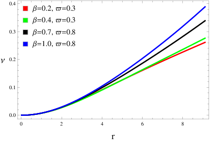
where μ˘\breve{\mu} is provided in Eqs.(41) and (66) with respect to each solution. The compactness of a geometrical structure primarily measures how intricate particles of that object are arranged, and we represent it as ν⁡(r)\nu(r) in this case. The tightness of these particles can be determined by calculating compactness factor, which is also defined by the mass-radius ratio. It was observed to be less than 49\frac{4}{9} by Buchdahl [38] for a spherical model. The noteworthy fact is that the wavelength of electromagnetic radiations in the neighborhood of a self-gravitating system is affected by its compactness. These radiations change their path from geodesic motion due to the gravitational attraction of the compact object. Such radiations are then redshifted which can mathematically be determined as

z⁡(r)={1−2​ν​(r)}−12−1,z(r)=\big\{1-2\nu(r)\big\}^{-\frac{1}{2}}-1, (70)

whose maximum value is observed as 2 and 5.211 for perfect [38] and anisotropic fluids [39], respectively.

In the field of astrophysics, it is interesting to know whether a compact structure incorporates an ordinary matter or not. The presence of such a fluid and viability of the resulting model can be guaranteed by the fulfillment of energy conditions. On the other hand, if any of these bounds does not satisfy then there must be an exotic matter inside the system. They have the following form in the considered setup

μ˘≥0,μ˘+P˘r≥0,\displaystyle\breve{\mu}\geq 0,\quad\breve{\mu}+\breve{P}_{r}\geq 0,
μ˘+P˘⊥≥0,μ˘−P˘r≥0,\displaystyle\breve{\mu}+\breve{P}_{\bot}\geq 0,\quad\breve{\mu}-\breve{P}_{r}\geq 0,
μ˘−P˘⊥≥0,μ˘+P˘r+2​P˘⊥≥0.\displaystyle\breve{\mu}-\breve{P}_{\bot}\geq 0,\quad\breve{\mu}+\breve{P}_{r}+2\breve{P}_{\bot}\geq 0. (71)

The obtained isotropic/anisotropic models which show stable behavior are considered as an important subject of discussion among all the celestial structures. Multiple techniques have been introduced in this regard to check the stability. Firstly, we use the causality condition according to which the inequalities 0<vs⊥2<10<v_{s\bot}^{2}<1 and 0<vs​r2<10<v_{sr}^{2}<1 should be satisfied to get stable behavior [40]. Here,

vs⊥2=d​P˘⊥d​μ˘,vs​r2=d​P˘rd​μ˘,v_{s\bot}^{2}=\frac{d\breve{P}_{\bot}}{d\breve{\mu}},\quad v_{sr}^{2}=\frac{d\breve{P}_{r}}{d\breve{\mu}},

are the tangential and radial sound speeds, respectively. If the absolute value of the difference between both the sound speeds, i.e., |vs⊥2−vs​r2||v_{s\bot}^{2}-v_{sr}^{2}| lies in the interval (0,1)(0,1), then the solution must be stable, named as the Herrera cracking concept [41]. Lastly, the adiabatic index (Γ\Gamma) is analyzed which states that the stable star must satisfy the inequality Γ>43\Gamma>\frac{4}{3} [42]. Here, Γ˘\breve{\Gamma} in terms of effective energy density and pressure is given as

Γ˘=μ˘+P˘rP˘r​(d​P˘rd​μ˘).\breve{\Gamma}=\frac{\breve{\mu}+\breve{P}_{r}}{\breve{P}_{r}}\bigg(\frac{d\breve{P}_{r}}{d\breve{\mu}}\bigg). (72)

We take a linear f⁡(ℝ,𝕋)f(\mathbb{R},\mathbb{T}) model (9) to explore deformation functions, the scalar 𝕐T​F\mathbb{Y}_{TF} and the effective state variables corresponding to different constraints through graphical analysis. We consider multiple choices of the decoupling and coupling parameters to study their role on physical attributes of a particular 4​U​1820−304U1820-30 model by fixing ℂ1=0.01\mathbb{C}_{1}=0.01 and g=0.003g=0.003. Figure 1 manifests graphs of the deformed gr​rg_{rr} metric function (39) showing increasing and non-singular trend for 0<r<ℛ0<r<\mathcal{R}. The parameters governing the matter distribution (such as pressure and energy density) are required to be maximum, positive and finite at the center, and show linear decrement towards the boundary to meet acceptability criteria of the developed model. We observe acceptable behavior of our first solution (41)-(44) from Figure 2. The upper left plot shows that the effective energy density is maximum in the core. Further, it decreases by increasing both the parameters ϖ\varpi and β\beta near the center, while shows opposite trend near the boundary. On the other hand, the pressure in both directions is observed to be in direct relation with ϖ\varpi as well as β\beta. The vanishing of the radial pressure at r=ℛr=\mathcal{R} can also be seen from the upper right plot. We transform anisotropic system to an isotropic for β=1\beta=1 that can be confirmed from the last plot, as the anisotropy is zero throughout for that value. Moreover, this factor shows increasing behavior for the remaining values of β\beta.

Refer to caption
Figure 1: Deformed gr​rg_{rr} component (39) for the solution corresponding to Π˘=0\breve{\Pi}=0.
Refer to captionRefer to captionRefer to captionRefer to caption
Figure 2: Matter variables and pressure anisotropy for the solution corresponding to Π˘=0\breve{\Pi}=0.
Refer to captionRefer to captionRefer to caption
Figure 3: Mass, compactness and redshift for the solution corresponding to Π˘=0\breve{\Pi}=0.
Refer to captionRefer to caption
Figure 4: Dominant energy conditions for the solution corresponding to Π˘=0\breve{\Pi}=0.
Refer to captionRefer to captionRefer to captionRefer to caption
Figure 5: Radial/tangential velocities, |vs⊥2−vs​r2||v_{s\bot}^{2}-v_{sr}^{2}| and adiabatic index for the solution corresponding to Π˘=0\breve{\Pi}=0.

Figure 3 (upper left plot) reveals that the isotropic system is initially less massive than anisotropic analog, but exhibits counter consequence towards the hypersurface. The compactness and redshift are plotted in the upper right and lower plots, respectively which meet their required limits. All the energy bounds must be fulfilled due to positive nature of the state variables except dominant conditions (μ˘−P˘r≥0\breve{\mu}-\breve{P}_{r}\geq 0 and μ˘−P˘⊥≥0\breve{\mu}-\breve{P}_{\bot}\geq 0), thus they are needed to be checked. Figure 4 assures validity of these conditions, hence our first solution is physically viabile. We check the stability by using three different approaches in Figure 5. The developed model (41)-(44) is unstable near the center for β=0.2\beta=0.2 (upper left plot) as well as near the boundary for β=1\beta=1 (upper two plots), while becomes stable for all the remaining considered choices of ϖ\varpi and β\beta . Meanwhile, the resulting solution is observed to be stable everywhere by using the adiabatic index and the cracking condition (lower two plots). Figure 6 indicates that the increment in both ϖ\varpi and β\beta decreases the complexity factors (51) and (62) which follows that the impact of complexity in f⁡(ℝ,𝕋)f(\mathbb{R},\mathbb{T}) theory is much lesser than that of 𝔾​ℝ\mathbb{GR}.

Refer to captionRefer to caption
Figure 6: Complexity factors (51) and (62).
Refer to caption
Figure 7: Deformed gr​rg_{rr} component (65) for the solution corresponding to 𝕐˘T​F=0\breve{\mathbb{Y}}_{TF}=0.

We adopt another constraint 𝕐˘T​F=0\breve{\mathbb{Y}}_{TF}=0 and obtain the corresponding solution (66)-(68) whose physical characteristics are analyzed by choosing ℂ3=0.01\mathbb{C}_{3}=0.01. Figure 7 provides the plot of deformed gr​rg_{rr} component presenting non-singular trend throughout. The matter variables and pressure anisotropy are analyzed in Figure 8 which show acceptable behavior as we have discussed earlier. The tangential pressure in this case is lesser than the radial component (except at the center), thus anisotropy appears to be negative throughout. Figure 9 (upper left) exhibits that the sphere becomes more massive by increasing both parameters ϖ\varpi and β\beta, in contrast to the result obtained through MGD. The right and lower plots confirm the acceptance of other two factors. Figure 10 discloses that our second solution as well as extended model (9) are also viable. Figure 11 reveals the stability of this solution everywhere.

Refer to captionRefer to captionRefer to captionRefer to caption
Figure 8: Matter variables and pressure anisotropy for the solution corresponding to 𝕐˘T​F=0\breve{\mathbb{Y}}_{TF}=0.
Refer to captionRefer to captionRefer to caption
Figure 9: Mass, compactness and redshift for the solution corresponding to 𝕐˘T​F=0\breve{\mathbb{Y}}_{TF}=0.
Refer to captionRefer to caption
Figure 10: Dominant energy conditions for the solution corresponding to 𝕐˘T​F=0\breve{\mathbb{Y}}_{TF}=0.
Refer to captionRefer to captionRefer to captionRefer to caption
Figure 11: Radial/tangential velocities, |vs⊥2−vs​r2||v_{s\bot}^{2}-v_{sr}^{2}| and adiabatic index for the solution corresponding to 𝕐˘T​F=0\breve{\mathbb{Y}}_{TF}=0.

7 Conclusions

The main objective of this paper is to extend some solutions for anisotropic self-gravitating distribution (𝕋η​ζ\mathbb{T}_{\eta\zeta}) through the addition of an extra source (𝔅η​ζ\mathfrak{B}_{\eta\zeta}) by employing gravitational decoupling scheme in f⁡(ℝ,𝕋)=ℝ+2​ϖ​𝕋f(\mathbb{R},\mathbb{T})=\mathbb{R}+2\varpi\mathbb{T} gravity. The corresponding field equations representing the total fluid configuration (seed and additional sources) have been formulated which are then split into two distinct sets by means of an EGD technique. Both sets of equations have ultimately represented their parent sources. For the first set describing seed source, we have taken the following metric potentials

χ⁡(r)=ln⁡{𝒜2​(1+r2ℬ2)},ρ⁡(r)=e−σ⁡(r)=ℬ2+r2ℬ2+3​r2,\chi(r)=\ln\bigg\{\mathcal{A}^{2}\bigg(1+\frac{r^{2}}{\mathcal{B}^{2}}\bigg)\bigg\},\quad\rho(r)=e^{-\sigma(r)}=\frac{\mathcal{B}^{2}+r^{2}}{\mathcal{B}^{2}+3r^{2}},

and the Tolman IV ansatz, resulting in two extended solutions. We have used the radius and mass of compact 4​U​1820−304U1820-30 model in order to determine three unknowns involving in these components. There have been five unknowns (ℱ,𝒢,𝔅00,𝔅11,𝔅22\mathcal{F},\mathcal{G},\mathfrak{B}_{00},\mathfrak{B}_{11},\mathfrak{B}_{22}) incorporated in Eqs.(22)-(24), thus we required to implement two constraints simultaneously to get the solution. We have considered a particular form of 𝒢⁡(r)\mathcal{G}(r) along with two independent constraints leading to first and second solution. One constraint has been taken as disappearance of the effective anisotropy for β=1\beta=1, therefore the system becomes an isotropic for this value. We have then implemented another limitation on the complexity, i.e., the total setup has been considered to be the complexity-free.

The role of modified gravity and gravitational decoupling on physical attributes of the developed models have been explored by choosing ϖ=0.3,0.8\varpi=0.3,~0.8 and β=0.2,0.4,0.7,1\beta=0.2,~0.4,~0.7,~1. The graphical interpretation of corresponding state determinants ((41)-(43) and (66)-(68)), anisotropic pressure ((44) and (A2)) and the energy constraints (71) have provided acceptable results for specific values of multiple constants. The redshift and compactness have also been shown to be within their required limits (Figures 3 and 9). We have observed that the obtained model corresponding to 𝕐˘T​F=0\breve{\mathbb{Y}}_{TF}=0 yields denser stellar structure, in comparison with the other solution. All the deformation functions have been found to be zero in the core of considered star and increasing towards the boundary. Further, the solution corresponding to Π˘\breve{\Pi} is stable throughout only for β=0.4,0.7\beta=0.4,~0.7 with causality condition, whereas the other solution is stable everywhere (Figures 5 and 11). The adiabatic index and Herrera’s cracking concept have provided stable structures, thus our obtained solutions are compatible with those of 𝔾​ℝ\mathbb{GR} [29]. The constraint Π˘=0\breve{\Pi}=0 has also been used in the the Brans-Dicke scenario to get solution which shows inconsistent behavior with f⁡(ℝ,𝕋)f(\mathbb{R},\mathbb{T}) gravity, as β=1\beta=1 provides unstable system in this case [31]. Finally, ϖ=0\varpi=0 reduces all of our results to 𝔾​ℝ\mathbb{GR}.

Appendix A

The value of ϱ1\varrho_{1} appearing in Eqs.(66)-(68) is

ϱ1\displaystyle\varrho_{1} =(ϖ+2π)(ϖ+4π){2(ϖ+1)r2g(βg(ℬ2−2𝒞2)+6)−(ϖ+1)g\displaystyle=(\varpi+2\pi)(\varpi+4\pi)\big\{2(\varpi+1)r^{2}g(\beta g(\mathcal{B}^{2}-2\mathcal{C}^{2})+6)-(\varpi+1)g
×(ℬ2+2𝒞2)ln(ℬ2+2r2)(ℬ2βg+4)+8ℂ3𝒞2+2(ϖ+1)βr4g2}\displaystyle\times(\mathcal{B}^{2}+2\mathcal{C}^{2})\ln\big(\mathcal{B}^{2}+2r^{2}\big)(\mathcal{B}^{2}\beta g+4)+8\mathbb{C}_{3}\mathcal{C}^{2}+2(\varpi+1)\beta r^{4}g^{2}\big\}
+2​π​ϖ​(ℬ2+2​𝒞2)r2−1(ℬ2+2​r2){2(ℬ2+2𝒞2)((ϖ+1)ϖ2ℬ2g\displaystyle+\frac{2\pi\varpi(\mathcal{B}^{2}+2\mathcal{C}^{2})}{r^{2}}-\frac{1}{(\mathcal{B}^{2}+2r^{2})}\big\{2(\mathcal{B}^{2}+2\mathcal{C}^{2})\big((\varpi+1)\varpi^{2}\mathcal{B}^{2}g
+6πϖ((ϖ+1)ℬ2g−1)+8π2((ϖ+1)ℬ2g−2))}−π​ϖ​2​ℬ2r3\displaystyle+6\pi\varpi((\varpi+1)\mathcal{B}^{2}g-1)+8\pi^{2}((\varpi+1)\mathcal{B}^{2}g-2)\big)\big\}-\frac{\pi\varpi\sqrt{2\mathcal{B}^{2}}}{r^{3}}
×(ℬ2+2​𝒞2)​tan−1⁡(2​rℬ2).\displaystyle\times(\mathcal{B}^{2}+2\mathcal{C}^{2})\tan^{-1}\bigg(\frac{\sqrt{2}r}{\sqrt{\mathcal{B}^{2}}}\bigg). (A1)

The anisotropy for our second solution (66)-(68) is

Π˘\displaystyle\breve{\Pi} =β8​π[2​g​(ℬ2+r2)​(r2−𝒞2)𝒞2​(ℬ2+2​r2)+g𝒞2​(ℬ2+2​r2)2{ℬ4(r2(g𝒞2−3)\displaystyle=\frac{\beta}{8\pi}\bigg[\frac{2g\big(\mathcal{B}^{2}+r^{2}\big)\big(r^{2}-\mathcal{C}^{2}\big)}{\mathcal{C}^{2}\big(\mathcal{B}^{2}+2r^{2}\big)}+\frac{g}{\mathcal{C}^{2}\big(\mathcal{B}^{2}+2r^{2}\big)^{2}}\big\{\mathcal{B}^{4}\big(r^{2}(g\mathcal{C}^{2}-3)
OPEN−r4​g+2​𝒞2)+ℬ2​(−3​r6​g+r4​(3​g​𝒞2−10)+7​r2​𝒞2)−2​r8​g\displaystyle-r^{4}g+2\mathcal{C}^{2}\big)+\mathcal{B}^{2}\big(-3r^{6}g+r^{4}(3g\mathcal{C}^{2}-10)+7r^{2}\mathcal{C}^{2}\big)-2r^{8}g
+2r6(g𝒞2−5)+8r4𝒞2}−2​ℬ2​r2+ℬ4+3​r48​(ℬ2+r2)​{(ϖ+2)​ℬ2+(2​ϖ+3)​r2}\displaystyle+2r^{6}(g\mathcal{C}^{2}-5)+8r^{4}\mathcal{C}^{2}\big\}-\frac{2\mathcal{B}^{2}r^{2}+\mathcal{B}^{4}+3r^{4}}{8\big(\mathcal{B}^{2}+r^{2}\big)\big\{(\varpi+2)\mathcal{B}^{2}+(2\varpi+3)r^{2}\big\}}
×(ϱ2𝒞2​(ϖ+2​π)​(ϖ+4​π)+8ℂ3)+{16(ϖ+2π)(ϖ+4π)\displaystyle\times\bigg(\frac{\varrho_{2}}{\mathcal{C}^{2}\big(\varpi+2\pi\big)\big(\varpi+4\pi\big)}+8\mathbb{C}_{3}\bigg)+\big\{16(\varpi+2\pi\big)\big(\varpi+4\pi\big)
×(ℬ2+r2)((ϖ+2)ℬ2+(2ϖ+3)r2)}−1(ℬ2+2r2){𝒞2(16ℂ3r2\displaystyle\times\big(\mathcal{B}^{2}+r^{2}\big)\big((\varpi+2)\mathcal{B}^{2}+(2\varpi+3)r^{2}\big)\big\}^{-1}\big(\mathcal{B}^{2}+2r^{2}\big)\bigg\{\mathcal{C}^{2}\big(16\mathbb{C}_{3}r^{2}
×((ϖ+2)​ℬ2+(2​ϖ+3)​r2)−16​(2​ϖ+3)​ℂ3​r2​(ℬ2+r2)+16​ℂ3\displaystyle\times\big((\varpi+2)\mathcal{B}^{2}+(2\varpi+3)r^{2}\big)-16(2\varpi+3)\mathbb{C}_{3}r^{2}\big(\mathcal{B}^{2}+r^{2}\big)+16\mathbb{C}_{3}
×(ℬ2+r2)((ϖ+2)ℬ2+(2ϖ+3)r2))(ϖ2+6πϖ+8π2)−2r2\displaystyle\times\big(\mathcal{B}^{2}+r^{2}\big)\big((\varpi+2)\mathcal{B}^{2}+(2\varpi+3)r^{2}\big)\big)\big(\varpi^{2}+6\pi\varpi+8\pi^{2}\big)-2r^{2}
×(2​ϖ+3)​ϱ2​(ℬ2+r2)+2​r2​ϱ2​((ϖ+2)​ℬ2+(2​ϖ+3)​r2)+2​ϱ2\displaystyle\times(2\varpi+3)\varrho_{2}\big(\mathcal{B}^{2}+r^{2}\big)+2r^{2}\varrho_{2}\big((\varpi+2)\mathcal{B}^{2}+(2\varpi+3)r^{2}\big)+2\varrho_{2}
×(ℬ2+r2)​((ϖ+2)​ℬ2+(2​ϖ+3)​r2)+r⁡(ℬ2+r2)​((ϖ+2)​ℬ2CLOSE\displaystyle\times\big(\mathcal{B}^{2}+r^{2}\big)\big((\varpi+2)\mathcal{B}^{2}+(2\varpi+3)r^{2}\big)+r\big(\mathcal{B}^{2}+r^{2}\big)\big((\varpi+2)\mathcal{B}^{2}
OPEN+(2​ϖ+3)​r2)​(4​(ϖ+1)​(ϖ2+6​π​ϖ+8​π2)​(ℬ2​β​g−2​β​g​𝒞2+6)CLOSE\displaystyle+(2\varpi+3)r^{2}\big)\bigg(4(\varpi+1)\big(\varpi^{2}+6\pi\varpi+8\pi^{2}\big)(\mathcal{B}^{2}\beta g-2\beta g\mathcal{C}^{2}+6)
×r​g+8​β​r3​g2​(ϖ+1)​(ϖ2+6​π​ϖ+8​π2)−4​π​ϖ​(ℬ2+2​𝒞2)r3\displaystyle\times rg+8\beta r^{3}g^{2}(\varpi+1)\big(\varpi^{2}+6\pi\varpi+8\pi^{2}\big)-\frac{4\pi\varpi(\mathcal{B}^{2}+2\mathcal{C}^{2})}{r^{3}}
−2​π​ϖ​ℬ2​(ℬ2+2​𝒞2)r3​(ℬ2+2​r2)+3​r−4​2​ℬ2​π​ϖ​(ℬ2+2​𝒞2)​tan−1⁡(2​rℬ2)\displaystyle-\frac{2\pi\varpi\mathcal{B}^{2}(\mathcal{B}^{2}+2\mathcal{C}^{2})}{r^{3}\big(\mathcal{B}^{2}+2r^{2}\big)}+3r^{-4}\sqrt{2\mathcal{B}^{2}}\pi\varpi(\mathcal{B}^{2}+2\mathcal{C}^{2})\tan^{-1}\bigg(\frac{\sqrt{2}r}{\sqrt{\mathcal{B}^{2}}}\bigg)
+8​r​(ℬ2+2​𝒞2)​(ℬ2+2​r2)−2​(6​π​ϖ​((ϖ+1)​ℬ2​g−1)+8​π2​((ϖ+1)CLOSECLOSE\displaystyle+8r(\mathcal{B}^{2}+2\mathcal{C}^{2})(\mathcal{B}^{2}+2r^{2})^{-2}\big(6\pi\varpi\big((\varpi+1)\mathcal{B}^{2}g-1\big)+8\pi^{2}((\varpi+1)
×ℬ2g−2)+(ϖ+1)ϖ2ℬ2g)−4(ϖ+1)(ℬ2+2r2)−1(ℬ2+2𝒞2)\displaystyle\times\mathcal{B}^{2}g-2)+(\varpi+1)\varpi^{2}\mathcal{B}^{2}g\big)-4(\varpi+1)(\mathcal{B}^{2}+2r^{2})^{-1}(\mathcal{B}^{2}+2\mathcal{C}^{2})
×rg(ϖ2+6πϖ+8π2)(ℬ2βg+4))}],\displaystyle\times rg\big(\varpi^{2}+6\pi\varpi+8\pi^{2}\big)(\mathcal{B}^{2}\beta g+4)\bigg)\bigg\}\bigg], (A2)

where

ϱ2\displaystyle\varrho_{2} =(ϖ+2π)(ϖ+4π){2(ϖ+1)r2g(βg(ℬ2−2𝒞2)+6)+2βg2\displaystyle=(\varpi+2\pi)(\varpi+4\pi)\big\{2(\varpi+1)r^{2}g(\beta g(\mathcal{B}^{2}-2\mathcal{C}^{2})+6)+2\beta g^{2}
×(ϖ+1)r4−(ϖ+1)g(ℬ2+2𝒞2)ln(ℬ2+2r2)(ℬ2βg+4)}\displaystyle\times(\varpi+1)r^{4}-(\varpi+1)g(\mathcal{B}^{2}+2\mathcal{C}^{2})\ln\big(\mathcal{B}^{2}+2r^{2}\big)(\mathcal{B}^{2}\beta g+4)\big\}
+2​π​ϖ​(ℬ2+2​𝒞2)r2−1(ℬ2+2​r2){2(ℬ2+2𝒞2)((ϖ+1)ϖ2ℬ2g\displaystyle+\frac{2\pi\varpi(\mathcal{B}^{2}+2\mathcal{C}^{2})}{r^{2}}-\frac{1}{(\mathcal{B}^{2}+2r^{2})}\big\{2(\mathcal{B}^{2}+2\mathcal{C}^{2})\big((\varpi+1)\varpi^{2}\mathcal{B}^{2}g
+6πϖ((ϖ+1)ℬ2g−1)+8π2((ϖ+1)ℬ2g−2))}−π​ϖ​2​ℬ2r3\displaystyle+6\pi\varpi((\varpi+1)\mathcal{B}^{2}g-1)+8\pi^{2}((\varpi+1)\mathcal{B}^{2}g-2)\big)\big\}-\frac{\pi\varpi\sqrt{2\mathcal{B}^{2}}}{r^{3}}
×(ℬ2+2​𝒞2)​tan−1⁡(2​rℬ2).\displaystyle\times(\mathcal{B}^{2}+2\mathcal{C}^{2})\tan^{-1}\bigg(\frac{\sqrt{2}r}{\sqrt{\mathcal{B}^{2}}}\bigg). (A3)

References

  • [1] Nojiri, S. and Odintsov, S.D.: Phys. Rep. 505(2011)59; Capozziello, S. et al.: Class. Quantum Grav. 25(2008) 085004; Nojiri, S. et al.: Phys. Lett. B 681(2009)74.
  • [2] Capozziello, S. et al.: Mon. Not. R. Astron. Soc. 394(2009)947; de Felice, A. and Tsujikawa, S.: Living Rev. Relativ. 13(2010)3.
  • [3] Sharif, M. and Kausar, H.R.: J. Cosmol. Astropart. Phys. 07(2011)022; Sharif, M. and Yousaf, Z.: Astrophys. Space Sci. 354(2014)471.
  • [4] Astashenok, A.V., Capozziello, S. and Odintsov, S.D.: J. Cosmol. Astropart. Phys. 01(2015)001; Phys. Lett. B 742(2015)160.
  • [5] Bertolami, O. et al.: Phys. Rev. D 75(2007)104016.
  • [6] Harko, T. et al.: Phys. Rev. D 84(2011)024020.
  • [7] Deng, X.M. and Xie, Y.: Int. J. Theor. Phys. 54(2015)1739.
  • [8] Houndjo, M.J.S.: Int. J. Mod. Phys. D 21(2012)1250003.
  • [9] Das, A. et al.: Phys. Rev. D 95(2017)124011.
  • [10] Deb, D. et al.: Phys. Rev. D 97(2018)084026.
  • [11] Sharif, M. and Siddiqa, A.: Eur. Phys. J. Plus 133(2018)226; Sharif, M. and Nawazish, I.: Astrophys. Space Sci. 363(2018)67; Sharif, M. and Naseer, T.: Eur. Phys. J. Plus 137(2022)1304.
  • [12] Rej, P., Bhar, Piyali. and Govender, M.: Eur. Phys. J. C 81(2021)316; Zubair, M. et al.: New Astron. 88(2021)101610; Azmat, H. and Zubair M.: Eur. Phys. J. Plus 136(2018)112.
  • [13] Ovalle, J.: Phys. Rev. D 95(2017)104019.
  • [14] Ovalle, J. et al.: Eur. Phys. J. C 78(2018)960.
  • [15] Sharif, M. and Sadiq, S.: Eur. Phys. J. C 78(2018)410.
  • [16] Sharif, M. and Saba, S.: Eur. Phys. J. C 78(2018)921; Chin. J. Phys. 59(2019)481; Sharif, M. and Waseem, A.: Ann. Phys. 405(2019)14.
  • [17] Estrada, M. and Tello-Ortiz, F.: Eur. Phys. J. Plus 133(2018)453.
  • [18] Hensh, S. and Stuchlík, Z.: Eur. Phys. J. C 79(2019)834.
  • [19] Ovalle, J.: Phys. Lett. B 788(2019)213.
  • [20] Contreras, E. and Bargueño, P.: Class. Quantum Grav. 36(2019)215009.
  • [21] Sharif, M. and Ama-Tul-Mughani, Q.: Ann. Phys. 415(2020)168122 ; Sharif, M. and Majid, A.: Phys. Dark Universe 30(2020)100610; ibid. 32(2021)100803; Sharif, M. and Aslam, M.: 81(2021)641.
  • [22] Zubair, M., Amin, M. and Azmat, H.: Phys. Scr. 96(2021)125008.
  • [23] Sharif, M. and Naseer, T.: Chin. J. Phys. 73(2021)179; Int. J. Mod. Phys. D 31(2022)2240017; Phys. Scr. 97(2022)055004; ibid. 97(2022)125016; Pramana 96(2022)119; Naseer, T. and Sharif, M.: Universe 8(2022)62.
  • [24] Herrera, L.: Phys. Rev. D 97(2018)044010.
  • [25] Herrera, L., Di Prisco, A. and Ospino, J.: Phys. Rev. D 98(2018)104059.
  • [26] Yousaf, Z., Bhatti, M.Z. and Naseer, T.: Eur. Phys. J. Plus 135(2020)353; Phys. Dark Universe 28(2020)100535; Int. J. Mod. Phys. D 29(2020)2050061; Ann. Phys. 420(2020)168267.
  • [27] Yousaf, Z. et al.: Phys. Dark Universe 29(2020)100581; Yousaf, Z. et al.: Mon. Not. R. Astron. Soc. 495(2020)4334; Sharif, M. and Naseer, T.: Chin. J. Phys. 77(2022)2655; Eur. Phys. J. Plus 137(2022)947.
  • [28] Carrasco-Hidalgo, M. and Contreras, E.: Eur. Phys. J. C 81(2021)757; Andrade, J. and Contreras, E.: Eur. Phys. J. C 81(2021)889; Arias, C. et al.: Ann. Phys. 436(2022)168671.
  • [29] Casadio, R. et al.: Eur. Phys. J. C 79(2019)826.
  • [30] Maurya, S.K. and Nag, R.: Eur. Phys. J. C 82(2022)48; Maurya, S.K. et al.: Eur. Phys. J. C 82(2022)100.
  • [31] Sharif, M. and Majid, A.: Eur. Phys. J. Plus 137(2022)114.
  • [32] Houndjo, M.J.S. and Piattella, O.F.: Int. J. Mod. Phys. D 2(2012)1250024.
  • [33] Moraes, P.H.R.S., Correa, R.A.C. and Ribeiro, G.: Eur. Phys. J. C 78(2018)192.
  • [34] Einstein, A.: Ann. Math. 40(1939)922.
  • [35] Clifton, T., Dunsby, P., Goswami, R. and Nzioki, A.M.: Phys. Rev. D 87(2013)063517.
  • [36] Goswami, R., Nzioki, A.M., Maharaj, S.D. and Ghosh, S.G.: Phys. Rev. D 90(2014)084011.
  • [37] Güver, T., Wroblewski, P., Camarota, L. and Özel, F.: Astrophys. J. 719(2010)1807.
  • [38] Buchdahl, H.A.: Phys. Rev. 116(1959)1027.
  • [39] Ivanov, B.V.: Phys. Rev. D 65(2002)104011.
  • [40] Abreu, H., Hernandez, H. and Nunez, L.A.: Class. Quantum Gravit. 24(2007)4631.
  • [41] Herrera, L.: Phys. Lett. A 165(1992)206.
  • [42] Heintzmann, H. and Hillebrandt, W.: Astron. Astrophys. 38(1975)51.