High Resolution Global Precipitation Downscaling with Latent Gaussian Models and Nonstationary SPDE StructureThanks: scastruc@nd.edu
Abstract
Obtaining high-resolution maps of precipitation data can provide key insights to stakeholders to assess a sustainable access to water resources at urban scale. Mapping a nonstationary, sparse process such as precipitation at very high spatial resolution requires the interpolation of global datasets at the location where ground stations are available with statistical models able to capture complex non-Gaussian global space-time dependence structures. In this work, we propose a new approach based on capturing the spatial dependence of a latent Gaussian process via a locally deformed Stochastic Partial Differential Equation (SPDE) with a buffer allowing for a different spatial structure across land and sea. The finite volume approximation of the SPDE, coupled with Integrated Nested Laplace Approximation ensures feasible Bayesian inference for tens of millions of observations. The simulation studies showcase the improved predictability of the proposed approach against stationary and no-buffer alternatives. The proposed approach is then used to yield high resolution simulations of daily precipitation across the United States.
Keywords: Latent Gaussian Model; Precipitation; Stochastic Partial Differential Equation; Integrated Nested Laplace Approximation
1 Introduction
Accurate high-resolution information of precipitation data is essential to effective prediction and management of water resources (Clark et al. 2015). Dramatic improvements in modeling physical processes driving precipitation have resulted in more realistic simulations from global climate models and hence more reliable predictions. The high complexity of modern climate models, however, implies a computational and storage cost which limit the spatial resolution at which global climate simulations can be performed. As such, there are significant uncertainties and mismatches with observations, due to precipitation patterns that coarse resolutions do not sufficiently represent as they cannot capture the scale of the physical processes of interest (Wood et al. 2021). The consequences can be over- or under-attribution of a particular location or incorrect timing of events, that can for example be the difference between a local flooding or not (Sapountzis et al. 2021). It is therefore of high scientific interest to refine global predictions and produce maps of both probability of rain occurrence and precipitation intensity at a high spatial scale, in order to inform impact assessment models for flood resilience and agricultural models for drought predictions.
It is in principle possible to produce high resolution precipitation using a coarse global dataset as boundary condition for a regional weather model such as the Weather and Research Forecasting (WRF, Skamarock et al. 2019). This dynamical downscaling approach (Sain et al. 2011) has the appealing advantage of producing physically consistent spatial fields at high resolution, but comes with a substantial associated cost in terms of computational and storage resources, as well as expertise for model setup that only few research centers, universities or businesses could afford. A more affordable solution lies in the formulation of an empirical relationship between global data and ground observations to be fit at locations where ground data are available. Under the assumption that this relationship is at least approximately valid at unobserved locations, high resolution maps can be produced by correcting the global dataset. This statistical downscaling approach (Berrocal et al. 2010) is fast, computationally affordable, and has a long established track record of success in the geoscience literature. In order to work, such approach requires that the global and the ground data are co-located, which is not a priori the case since global data are defined as averages over large areas. It becomes therefore necessary to use spatial statistical models to interpolate the global simulation values at the same locations of the ground observations, and to have an assessment of the uncertainty around these estimates.
Global spatial data require the formulation of specialized models whose theoretical properties are substantially different from spatial processes on Euclidean spaces. In fact, Gneiting 2013 highlighted how a valid process on the sphere with great circle distance could be achieved only with severe restrictions on the parameter space of the most widespread covariance model, the Matérn function. In the past two decades, new modeling approaches tailored for global data have emerged. Among them, Jun and Stein 2007; Jun and Stein 2008 proposed to embed the sphere in a three dimensional space, consider a Matérn model and apply partial derivatives to achieve more flexibility. The proposed class of models was able to capture not just an isotropic behavior, but also axial symmetry, i.e., a nonstationary behavior across latitude (Jones 1963). Jun 2011 generalized this approach to multivariate global processes. A fast and flexible spectral class of axially symmetric models was proposed in the case of gridded data by Castruccio and Stein 2013. The approach was then generalized to non-parametric spectral estimation (Castruccio and Genton 2014), three-dimensional variables (Castruccio and Genton 2016), different land/ocean behavior (Castruccio and Guinness 2017) and also multivariate processes (Edwards et al. 2019). On the more theoretical side, substantial progress has been made in the determination of properties of high dimensional spheres for isotropic processes via basis decomposition see, e.g., Arafat et al. 2020; Porcu et al. 2020. We refer to Jeong et al. 2017; Porcu et al. 2018 for two recent reviews on the topic.
A novel, different perspective was raised in the seminal work of Lindgren et al. 2011, where a subclass of Matérn models was associated with the solution of a diffusion-reaction Stochastic Partial Differential Equation (SPDE) with the Markov property and inference was performed with finite volumes. The key insight of this approach, as far as global models are concerned, is that the original SPDE on the plane can be just adapted to the sphere, with the additional benefit of not requiring boundary conditions. While in its original formulation the SPDE resulted in stationary models, non-stationary extensions have been proposed by allowing spatially varying coefficients. Several alternatives have been proposed, from nested SPDE (Bolin and Lindgren 2011) to models with physical barriers (Bakka et al. 2019). Recently, Fuglstad et al. 2015; Fuglstad and Castruccio 2020 extended this approach by allowing models with local deformation of the SPDE via a spatially varying scalar and vector field. The proposed approach showed promising results, but has been so far limited to the Gaussian case and generalization to non-Gaussian data is by no means straightforward, given the challenges in modeling non-Gaussian data and the computational overhead implied by these models.
In this work, we propose a non-Gaussian, non-stationary SPDE-based global spatio-temporal model with local deformation and a buffer between land and sea to account for abrupt changes in spatial dependence. Non-Gaussianity is modeled via a latent Gaussian model, i.e., by assuming that the non-Gaussian marginal behavior is conditionally independent across locations, and then the spatial dependence is captured via a latent process with a Gaussian structure. Inference is still achievable for very large datasets by means of 1) a sparse precision matrix of the latent Gaussian model emerging from the finite volume solution of the SPDE and 2) a fast approximation of the high-dimensional integrals required for posterior computation via Integrated Nested Laplace Approximation (INLA, Rue et al. 2009). The model is ideally suited to highly non-Gaussian data such as daily global precipitation, and it is then used to 1) fit global reanalysis data, 2) provide interpolated data at the same location as the ground observations, 3) downscale precipitation using both ground and interpolated data, so that 4) high resolution maps of precipitation are provided.
The work proceeds as follows. Section 2 introduces the data which will be used in this work. Section 3 details the methodology for the latent Gaussian model, specifically the temporal and the spatial component. Section 4 shows how inference is performed and how sparsity and numerical approximations alleviate the computational burden. Section 5 assesses numerically the posterior consistency, as well as the improved predictability of the proposed model against simpler alternatives. Section 6 applies the proposed model to the precipitation data and shows it can provide high resolution maps of daily precipitation across the continental United States. Section 7 concludes with a discussion. For reproducibility, at the end of this work we provide information about the repository where the code and data are available.
2 Data Description
We focus on daily global precipitation data from the Modern-Era Retrospective Analysis for Research and Applications, version 2 (MERRA-2, Gelaro et al. 2017) produced by the NASA Global Modeling and Assimilation Office (GMAO). MERRA-2 is a reanalysis data product that incorporates observations from satellite instruments and is considered one of the best representations of the state of the Earth’s system. The data is available on a regular grid with a resolution of in longitude and latitude, respectively, for a total of locations. We focus on the year 2021, the latest year with a continuous record available, and we use the daily Maximum Rainfall Rate (MRR, in . To convert the MRR into precipitation, we divided it by the water density, 1,000 , and convert the unit to millimeter by multiplying by 1,000, as well as multiply by 86,400 to obtain the daily precipitation. We assume that for each location, the MRR lasts for the whole day, which leads to some overestimation, as it can be clearly seen from the two different legend scales in Figure 1. The downscaling approach in Section 6 will be able to account for this by performing a linear transformation between (interpolated) MERRA-2 and USCRN.

For ground observations, we consider the U.S. Surface Climate Reference Network (USCRN, NOAA 2022), a data product containing continuous records from climate monitoring stations across the continental United States. The USCRN monitoring stations record measurements for total precipitation, measured in millimeters (mm), in real-time in 5-minute intervals. The data are collected with a Geonor T-200B precipitation gauge, whose maximum capacity is 600mm. This gauge uses a precipitation collection bucket which is surrounded by a wind/snow shield and heated in order to prevent ice buildup in cold regions. Three wires attached to this collection device vibrate with frequencies relative to the weight of the bucket, and these vibration frequencies are then converted to gauge depth (in mm). For this work, we consider data from 131 different monitoring stations post-processed to daily resolution forming a continuous record from January , 2021 to December, 31 2021. Figure 1 shows the locations of the USCRN sensors along with the average total daily precipitation throughout 2021. For comparison, the same figure also shows the average daily precipitation for the MERRA-2 grid points during the same time frame. It is readily apparent from this Figure that the regions of highest average daily precipitation are the northwest and southeast regions of the country whereas the drier region of the country spans from the eastern border of California through to the Mississippi River.
3 Methodology
3.1 Latent Gaussian Model
We propose a spatio-temporal latent Gaussian model (Rue et al. 2009), defined for a generic spatial point on the sphere and time as:
| (1a) | ||||
| (1b) | ||||
| (1c) | ||||
where represents the marginal distribution of conditional on the latent field and the hyperparameters, and belongs to the exponential family with some mean , whose structure is determined by a latent Gaussian process through a link function . The marginal parameters characterize moments higher than the first, and could be empty. If the marginal distribution is Gaussian, we have , and the link function is simply the identity function (Dunn and Smyth 2018). For example, if the marginal distribution is the Bernoulli distribution instead, we have , and the logit function can be chosen as the link function (Dunn and Smyth 2018). We assume that the transformed mean in the latent space is modeled by a location specific time effect, , location-specific covariates , and a spatial error . The time effect is described by harmonics with parameters and . If we assume that we have a sample observed at , the total number of temporal parameters in equation (1c) is , where , for a total of parameters. The period depends on the leap/no-leap year considered. We assume that the spatial random effect is a realization from a mean-zero Gaussian random field independent in time, whose covariance function depends on some parameters which will be specified in the next Section.
3.2 Spatial Correlation Structure
The simplest models for the spatial dependence of are stationary and isotropic, i.e., they assume that the dependence is a function of . Among them, one of the most popular choices is arguably the Matérn model, whose correlation between two locations is defined as (Stein 1999)
where is the modified Bessel function of the second kind with smoothness parameter (i.e., controlling the degree of mean squared differentiability) and range parameter . If inference is sought for a large dataset, a matrix comprising of the covariance among all locations could not be stored, and likelihood evaluation could become computationally challenging or just impossible. Instead of operating directly with the covariance matrix, a popular solution in the past decade has been to rely on the identification of a Gaussian process with Matérn covariance as the (unique) stationary solution of the following fractional reaction diffusion SPDE (Whittle 1954):
| (2) |
where is the Laplacian operator and is a spatial Gaussian white noise. By exploiting an ‘explicit link’ between a continuous Markov process when is integer in (2) and a discrete Gaussian Markov Random Field (GMRF), Lindgren et al. 2011 proved that if all locations are arranged on a 2D lattice, then the covariance structure of the GMRF could be approximated by applying the convolution of a sparse precision matrix. Moreover, any location that is not on the lattice could also be interpolated and approximated by means of a triangulation over the domain. Ultimately, this implies that the Matérn covariance can be approximated by a sparse precision matrix, and hence allow faster and feasible inference on the spatial structure of . In this work, we rely on a similar SPDE defined on a sphere defined as
| (3) |
where is the Laplacian operator.
The aforementioned SPDE approach has clear computational advantages, but in its formulation is limited to stationary and isotropic processes (Rue et al. 2009). The SPDE operator can, however, be generalized to allow for nonstationary constructs, while still yielding sparse precision matrices. In this work we rely on a spatially varying SPDE originally formulated in Fuglstad et al. 2019, but other approaches for spatially varying parameters (Rue et al. 2009) or nested SPDE (Bolin and Lindgren 2011) have been proposed. We assume a location on the sphere has polar coordinates , where is the latitude and is the longitude. We introduce two terms: a vector field and a positive-valued scalar field . We then define the inverse deformation tensor as:
One can show that with the spatially varying metric tensor defined above, the distance along the direction is scaled by . In the orthogonal direction of , the distance is scaled by . Therefore, the vector field specifies the direction of the local anisotropic effect at each location, while represents its strength. After specifying the metric tensor , it case be shown that an appropriate change of variable in the SPDE (3) yields (Fuglstad and Castruccio 2020):
| (4) |
3.3 Spherical Harmonics
Both the vector field and the scalar field can be specified through basis decomposition such as spherical vector harmonics and spherical harmonics, respectively. However, a more flexible approach is necessary for global models, which must account not just for slowly changing nonstationarity, but also for abrupt changes dictated by large geographical descriptors such as land and ocean (Castruccio and Guinness 2017). In order to formulate a valid model via SPDE while still accounting for abrupt changes, we consider the buffering approach proposed by Bakka et al. 2019. More specifically, we use a buffer area along coastlines with a separate parameter that describes the multiplicative drop in the strength of dependence in the buffer area, so that for each of the land/ocean domain we propose a separate spherical harmonics decomposition:
where are real-valued coefficients and are Laplace’s spherical harmonic of degree and order and specifies the geographical descriptor where is located. Similarly, the vector field can be described as:
where is the unit vector in the positive radial direction, and are real coefficients, is the highest order in the bases. Additionally, in order to account for micro-scale variability, we assume that the process for both land and sea also has a nugget . In summary, the spatial parameters of the model are , for a total of parameters.
We use a priori independent standard normal distributions as priors for all parameters, with log transformation if they are constrained to be positive. The same setting is applied to the parameters used in simulation study and application.
4 Inference
We propose a stepwise inference approach to reduce the overall dimension of the parameter space in each step. We first estimate at each location independently, then conditionally on the temporal parameters. In Edwards et al. 2020 it was shown that the stepwise approach results in an asymptotically consistent inference, and Castruccio and Guinness 2017 showed that uncertainty and bias propagation have small impact for large yet finite datasets such as the one we work with here.
4.1 Step 1: Temporal Structure
In the first step, the inference is performed at each location independently without spatial and covariate effect. We redefine equation (1) as the following:
| (5) |
The vector of temporal parameters and the linear parameters are estimated using least-squares and the parameters are considered fixed in the following inference steps. Once are obtained, conditional on them the spatial parameters of the spatial process can be estimated.
4.2 Step 2: Spatial Covariance Structure
We define a collection of triangles on the sphere, and use a finite volume method to discretize the SPDE in (4). We redefine the inverse matrix tensor as , where , and we integrate it over triangles generated on a global mesh and seek for a piece-wise constant solution to the SPDE. For all triangles , we have the following equality in distribution:
| (6) |
Here is the divergence operator, is the gradient operator, and is a piecewise continuously differentiable diffusion tensor and is the surface measure on the triangles. This allows to translate the SPDE into a set of linear equations for a Gaussian vector that is assumed to be constant across each triangle.
Similarly to Bertolazzi and Manzini 2007; Fuglstad and Castruccio 2020, let be the vector of values at triangle center, then the following matrix could be calculated to describe a discrete approximation:
Here, represents the three faces of the triangle . Then, we combine this with a diagonal matrix , in which , so that we have:
With this approximation, the equality in distribution expressed in equation (6) can now be expressed as:
where is a diagonal matrix with elements . This implies that , and is a sparse precision matrix defined as:
Therefore, the finite volume method ensures a sparse precision matrix, which mitigates the computational burden for large global data and boosts the computing speed of the nonstationary model during inference.
4.3 Inference for Latent Gaussian model
In order to perform inference on the latent Gaussian Model, in this work we make use of the Nested Laplace Approximation (INLA, Rue et al. 2009) a method for Bayesian inference alternative to traditional Markov Chain Monte Carlo (MCMC), which could further ease the computational burden. INLA is a deterministic method for fast approximation of high dimensional integrals which takes advantage of computational properties of models that can be expressed as a latent GMRF. Thus, the INLA approach is used for performing the inference in this study. Under the proposed latent Gaussian Model structure, we have the observed data vector denoted here as at locations that can be described by hyperparameter vector . For simplicity, throughout this section, we will use to represent hyperparameter vector . If conditioned on latent spatial field , the observations are marginally independent with likelihood:
where is a Gaussian field with mean zero and modeled by a SPDE approach with precision matrix . Therefore, the joint distribution of latent effect and hyperparameters can be written as:
where is the determinant of the precision matrix. The main goal is to approximate the posterior marginals , and . The marginal posterior distributions of interest can be written as:
The key idea of INLA approach is to use the form above to construct nested approximations. The approximations of the marginals for the latent field are computed by approximating and , and using numerical integration to integrate out . In other words, the posterior marginals of the latent parameter would be obtained by:
where are the weights associated with a vector of hyperparameters in a grid.
5 Simulation Studies
Throughout this section, we denote with NS-LS the proposed nonstationary latent Gaussian model (4) with land/sea effect with NS the nonstationary model with no land/sea effect. We further consider the stationary SPDE model (3), and denote with S-LS the model with land/sea effect and with S without it. In Section 5.1, we perform simulations from the Gaussian marginal distribution for NS-LS to numerically assess posterior consistency for both the hyperparameters and the resulting covariance matrix. In Section 5.2 and Section 5.3, we perform simulations from Gaussian and Bernoulli marginal distributions with identity and logit link, respectively, to assess the interpolation (kriging) performance of the NS-LS against NS, S-LS and S.
Since the key contribution of this work lies in the spatial component of the model, throughout this section we will assume a purely spatial process with no covariates. In other words, model (1) simplifies to
| (7a) | ||||
| (7b) | ||||
In the Gaussian case we also have , while in the Bernoulli case no marginal parameters are defined, so that .
For each simulation, we sample data points on the unit sphere, and then draw the parameters of from a Normal distribution with mean 1 and standard deviation 0.5, assume them fixed (similar results have been observed for other samples or distributions). Each simulation comprises of replicates from the resulting covariance matrix . We simulate data from a NS-LS model with , so that there is a total of hyperparameters. We perform independent simulations and report the results both in terms of aggregated performance and their uncertainty .
5.1 Posterior consistency in the Gaussian case
In order to numerically assess posterior consistency, for each simulation we consider an increasing number of replicates . Inference is performed assuming the same model (7) and with a mesh of triangles. For varying levels of , the hyperparameters’ posterior distributions is retrieved and is compared with the true value. Posterior consistency can be empirically verified in the extent to which the hyperparameters’ posterior distributions converges to the true parameters as increases.

| 20 | 40 | 60 | 80 | 100 | |
| Median MSE (IQR) | 0.32 (0.13) | 0.25 (0.07) | 0.14 (0.05) | 0.05 (0.05) | 0.01 (0.007) |
Figure 2 shows the functional boxplot (Sun and Genton 2011) for all of the posterior distributions, for two hyperparameters for increasing values of realizations . It is readily apparent how the posterior mean aligns to the true parameter value and the posterior standard deviations decreases as the replicates increase. While results are shown for NS-LS, similar patterns have been observed across all other models (NS, S-LS and S). Table 1 shows the median MSE and InterQuartile Range (IQR) of the hyperparameters posterior means estimated from the NS-LS model and the true values across all hyperparameters and across all simulations. The median MSE decreases as the replicates increases.
In order to perform a uniform comparison across all hyperparameters, whose number quickly becomes overbearing (e.g., with we would have hyperparameters), we also compare the covariance matrix implied by the hyperparameters with the true one. We assess the discrepancy in the covariances via the Kullback-Leibler Divergence (KLD), which in the case of an -dimensional Gaussian distributions with mean and and covariance matrices and simplifies to:
In our case , and , so that the KLD measures the distance between the true and estimated covariance. The results as shown in Figure 3 for NS-LS (panel (a)) and S (panel (b)), where the functional boxplot (Sun and Genton 2011) of KLD across all simulations for an increasing number of realizations is shown. The functional boxplot is used to report the envelope of the 50% central region (pink area), the median curve (black line) and the maximum non-outlying envelope (outer blue line). As in the case of the estimated parameters, we observe how even with a relatively small number of replicates in the training set, the estimated covariance is converging to the true one. In particular, after 40 replicates the estimated covariance is practically indistinguishable from the true one.

5.2 Interpolation performance in the Gaussian case
In order to assess the interpolation performance, we perform inference on the hyperparameters for all four models and use them to interpolate at specified locations. We consider two cases (1) all data points are used in the training set and interpolation is performed at the same sites (2) 92% of the locations are considered in the training set, and the others 8% are withheld for crossvalidation. The test locations are located in within three selected areas indicated in Figure S1. Interpolation performance is measured with the MSE.
Results for both cases are reported in Table 2, and it is readily apparent how the MSE of NS-LS model is the smallest among all four models for the both the all location case (1) and the cross-validation setting (2). More specifically, compared to the S-LS model, the NS-LS model shows an improvement of the median MSE across all locations by 14.6%. The NS-LS model also shows an appreciable improvement in MSE by 10.4% and 16.7%, compared with the NS and S models respectively. From these results it is clear how the land/sea effect and buffer area construction yield significant improvement when used in conjunction with the NS model.
| Model | locations | NS-LS | S-LS | NS | S |
| Gaussian | All locations | 90.12 (8.17) | 105.47 (9.94) | 100.55 (11.25) | 108.25 (11.23) |
| Crossvalidation | 9.11 (1.04) | 21.88 (1.18) | 19.35 (1.62) | 21.39 (1.59) | |
| Bernoulli | All locations | 0.824 (0.048) | 0.769 (0.074) | 0.782 (0.051) | 0.753 (0.050) |
| Crossvalidation | 0.707 (0.072) | 0.676 (0.081) | 0.672 (0.079) | 0.641 (0.079) |
5.3 Interpolation performance in the Bernoulli case
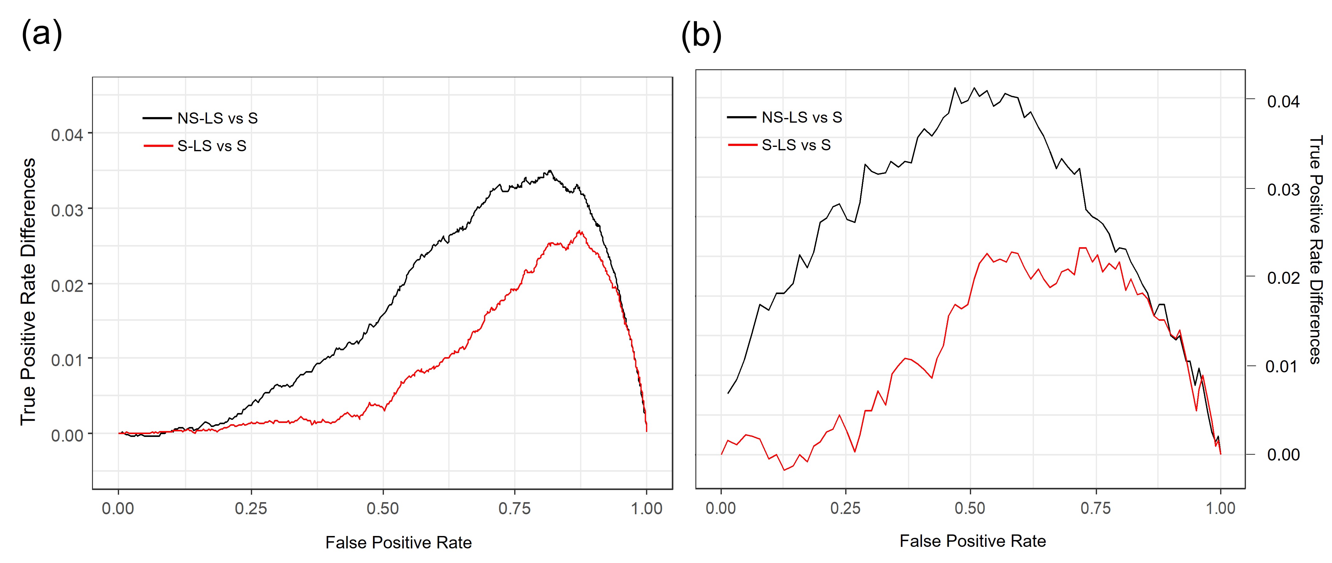
We now assess predictability in the case of a Bernoulli distribution with logit link, and as in Section 5.2 we assess both the case where all locations are used as training set, as well as cross-validation with the same testing locations as before. Figure 4 shows the average differences across all simulations between receiver operating characteristic curve (ROC) for NS-LS and S-LS, using S as reference for all locations and validation locations. The ROC for NS are visually indistinguishable to that of the S-LS model, so the results associated to that model are not show. The ROC difference in both cases show how the NS-LS model is uniformly better than the stationary S model (as the ROC difference is always positive), and also uniformly better than the S-LS model, especially in the middle of the curve. As expected, the extent of improvement of NS-LS is larger in the case of cross-validation (panel (b)), where the added value of the model at unobserved locations is more apparent.
In order to have a comprehensive assessment across all possible choice of thresholds, we consider the area under the curve (AUC) of the ROC for all models and we report it in Table 2. In the best case of a perfect prediction, i.e., 100% true positive rate uniformly across the choice the threshold the AUC should equal 1, and in the worst case of a random guess it should be 0.5. The extent to which the AUC is close to 1 is a measure of predictive performance in this case. As it is shown in Table 2, the NS-LS outperforms every other model in both cases. More specifically, across all locations, the NS-LS yields an improvement by 7.2%, 5.3% and 9.4% for the S-LS, NS and S models respectively. These results agree with those presented in Section 5.2, for the use of the land/sea effect and buffer area construction definitively yields improved performance when included in the NS model.
6 Application
In this section, we use the data detailed in Section 2 and the proposed latent Gaussian model with nonstationary SPDE introduced in Section 3 to estimate the global probability of a rain event and the precipitation intensity. In section 6.1, we discuss both the fit of the global MERRA-2 dataset and the downscaling approach to adjust interpolated MERRA-2 data with ground USCRN precipitation measurement. In section 6.2, we provide evaluation metrics to assess the model performance.


6.1 Modeling global precipitation and downscaling
We initially focus on the MERRA-2 data and consider two global data sets 1) a binary rain occurrence event and 2) in case of rain, the actual rain intensity. We then fit the latent Gaussian model (1) with nonstationary PDE (4) with , using a Bernoulli marginal distribution with a logit link function for rain occurrence and a Gamma distribution with negative inverse link function for rain intensity. Validation for the choice of the marginal distribution can be found in the supplementary along with Figure S3 showing the histogram of precipitation at 456 sample locations (resolution of in longitude and latitude) with estimated Gamma density. The sample locations are sparse in space to mitigate any spatial influences.
In both cases, no additional covariates are assumed, and we assume harmonics for the temporal component, as it was shown to be the optimal choice according to the model selection in Figure S2. Formally, model (1) now specializes in the following two models:
| (8a) | |||
| (8b) | |||
The histogram shows that precipitation intensity follows a Gamma distribution with shape parameter 0.826 and scale parameter 0.184. Inference is performed with a global triangulation of triangles, of which are within the area of interest (contiguous United States), while the remaining cover the rest of the world.
The hyperparameters’ posterior distributions is obtained and used to predict both the precipitation probability and intensity at the locations where the 131 USCRN ground observations locations are located, see Figure 1. These predictions are then adjusted (downscaled) to point resolution via linear regression. Since we perform downscaling independently for every time point, for simplicity we now drop the time dependence, and we denote as and the precipitation intensity for USCRN and MERRA2, respectively (G=ground, S=simulation), and with and the probability of precipitation occurrence. We further denote as and the estimated intensity and probability of occurrence, respectively, according to the proposed SPDE model. Finally, we estimate the probability of precipitation occurrence for the USCRN data by fitting the latent Gaussian model (1) for each location independently as a time series model, i.e., assuming no spatial dependence and denote the estimate as . We further assume a linear relationship between USCRN and MERRA2 precipitation occurrence probability and intensity:
| (9a) | |||
| (9b) | |||
where independent and identically distributed in space. A functional boxplot of the variogram of the residuals in Figure S4 (with each curve representing a different time point) lends support to the assumption of spatial independence of the error. The downscaling parameters and for precipitation intensity are then estimated using the ordinary least squares.
6.2 Results and Evaluation
Downscaled probabilities of precipitation occurrence and precipitation intensity according to the aforementioned model are displayed in Figure 5(a) and (b), respectively, with the dark bubbles representing average values from the USCRN data. The prediction maps of the United States show high daily precipitation and high precipitation intensity around Seattle, while the lowest values can be found near Las Vegas, and overall the model prediction resembles the ground observation values across the United States. To evaluate the model performance, we calculate the root mean squared error (RMSE) for both probability of precipitation occurrence and precipitation intensity. The RMSE for intensity and probability of precipitation occurrence is 2.01 mm and 0.14 mm, respectively. In order to assess the value added by the smoothing of our SPDE model, we also perform downscaling with the linear models in (9), but assuming that no spatial model is fit, i.e., that the MERRA-2 data are not interpolated at the locations of the USCRN sites. Instead, we consider MERRA-2 data at their original resolution, and attribute to each USCRN site the value in the same cell. In other words, we consider as covariates and . The resulting RMSE for this model in the case of precipitation intensity and probability of precipitation occurrence is 82.74 mm and 0.28 mm, respectively. Therefore, the proposed SPDE approach has narrowed the discrepancy between MERRA-2 and USCRN significantly, as it has reduced the RMSE for precipitation intensity and probability of precipitation occurrence by 97.6% and 50%, respectively. Figure 6 shows the fitted lines using downscaling model in (9a) and (9b) on February , 2021. The for the two linear models are 0.78 and 0.67 for precipitation probability and intensity, respectively.
We also evaluate the model uncertainty by crossvalidation. First, we remove the data from one ground observation location and fit the model using the remaining observations. Next, we construct the 95% credibility interval for the posterior mean of the probability of precipitation occurrence or precipitation intensity at the removed location with the estimated posterior distributions of the hyperparameters of the model. Then, we repeat the same procedure for all the 131 locations in USCRN. Finally, we determine how many intervals among the 131 the 95% credibility intervals cover the true value. For precipitation, 93.1% (122/131) of the 95% credibility intervals cover the true value, while for probability of raining, 91.6% (120/131) of the 95% credibility intervals cover the true value.
7 Conclusion and Discussion
In this work, we have proposed a novel non-stationary spatio-temporal SPDE model able to smooth both probability of precipitation occurrence and probability intensity from a global datasets. Such interpolated dataset is then used in conjuction with ground observation to produce high resolution (downscaled) precipitation maps, which allow to predict what would ground observations would look like in unsampled location with a higher degree of accuracy compared to the original simulated data (i.e., the global data at their native resolution). One may in principle use MERRA-2 as a boundary condition to drive regional simulations with models such as WRF to obtain precipitation maps at equally high spatial resolution, with the added benefit of being able to produce predictions compliant with physical laws. Such dynamical downscaling approach is however considerably more involved as it require substantial computational and storage resources, as well as considerable expertise to set up WRF properly. As such, our proposed statistical downscaling approach is considerably faster and easier to implement without specialized computational resources. The proposed method of adjustment of a simulation via ground observation can also be seen as a bias correction approach, i.e., a method to correct simulations (see, e.g., Yuan et al. 2019; Kim et al. 2015 and Ho et al. 2012; Hawkins et al. 2013 for a general review). While a large body of literature in geoscience focuses on bias correction as a means to adjust the first (Hemer et al. 2012; Chen et al. 2012) and possibly the second moment (Teutschbein and Seibert 2012; Li et al. 2019) of the marginal distribution, such approach can be used also to adjust non-Gaussian features, similarly to other recent efforts (Piani and Haerter 2012; Vrac and Friederichs 2014).
The proposed statistical model is scalable to future reanalysis data products with even higher spatial resolution, owing to the finite volume approximation of the SPDE generating the spatial model. Even more realistic downscaled patters could be generated if additional physical variables such as temperature and humidity could be considered as covariates. An incorporation of covariates could be performed either as the latent Gaussian model in (1b), as suggested in this work, or as as additional input of the scalar or vector field which dictate the deformation of the SPDE model. This could be implemented assuming either a linear contribution, or a non-linear one by means of neural networks (Hu et al. 2022). In principle, multiple variables could be modeled jointly. However, this would considerably increase both the methodological challenge and the computational overhead, as fast, flexible, multivariate and non-Gaussian global models are currently an active area of investigation (Genton and Kleiber 2015).
Acknowledgements
This research is supported by grant NSF DMS 2014166.
References
- Arafat et al. [2020] Ahmed Arafat, Pablo Gregori, and Emilio Porcu. Schoenberg coefficients and curvature at the origin of continuous isotropic positive definite kernels on spheres. Statistics & Probability Letters, 156:108618, 2020. ISSN 0167-7152. doi: https://doi.org/10.1016/j.spl.2019.108618.
- Bakka et al. [2019] Haakon Bakka, Jarno Vanhatalo, Janine B. Illian, Daniel Simpson, and Håvard Rue. Non-stationary gaussian models with physical barriers. Spatial Statistics, 29:268–288, 2019. ISSN 2211-6753. doi: https://doi.org/10.1016/j.spasta.2019.01.002. URL https://www.sciencedirect.com/science/article/pii/S221167531830099X.
- Berrocal et al. [2010] V.J. Berrocal, A.E. Gelfand, and D.M. Holland. A spatio-temporal downscaler for output from numerical models. Journal of Agricultural Biological and Environmental Sciences, 15:176–197, 2010.
- Bertolazzi and Manzini [2007] Enrico Bertolazzi and Gianmarco Manzini. On vertex reconstructions for cell-centered finite volume approximations of 2d anisotropic diffusion problems. Mathematical Models and Methods in Applied Sciences, 17(01):1–32, 2007. doi: 10.1142/S0218202507001814. URL https://doi.org/10.1142/S0218202507001814.
- Bolin and Lindgren [2011] David Bolin and Finn Lindgren. Spatial models generated by nested stochastic partial differential equations, with an application to global ozone mapping. The Annals of Applied Statistics, 5(1):523 – 550, 2011. doi: 10.1214/10-AOAS383. URL https://doi.org/10.1214/10-AOAS383.
- Castruccio and Genton [2014] Stefano Castruccio and Marc G. Genton. Beyond axial symmetry: An improved class of models for global data. Stat, 3(1):48–55, 2014.
- Castruccio and Genton [2016] Stefano Castruccio and Marc G. Genton. Compressing an ensemble with statistical models: An algorithm for global 3d spatio-temporal temperature. Technometrics, 58(3):319–328, 2016.
- Castruccio and Guinness [2017] Stefano Castruccio and Joseph Guinness. An evolutionary spectrum approach to incorporate large-scale geographical descriptors on global processes. Journal of the Royal Statistical Society. Series C (Applied Statistics), 66(2):329–344, 2017. ISSN 00359254, 14679876. URL http://www.jstor.org/stable/44682577.
- Castruccio and Stein [2013] Stefano Castruccio and Michael L. Stein. Global space–time models for climate ensembles. The Annals of Applied Statistics, 7(3):1593 – 1611, 2013. doi: 10.1214/13-AOAS656. URL https://doi.org/10.1214/13-AOAS656.
- Chen et al. [2012] Lian Chen, S. C. Pryor, and Dongliang Li. Assessing the performance of intergovernmental panel on climate change ar5 climate models in simulating and projecting wind speeds over china. Journal of Geophysical Research: Atmospheres, 117:D24102, 2012. doi: 10.1029/2012JD017533. URL https://agupubs.onlinelibrary.wiley.com/doi/abs/10.1029/2012JD017533.
- Clark et al. [2015] Martyn P Clark, Ying Fan, David M Lawrence, Jennifer C Adam, Diogo Bolster, David J Gochis, Richard P Hooper, Mukesh Kumar, L Ruby Leung, D Scott Mackay, et al. Improving the representation of hydrologic processes in earth system models. Water Resources Research, 51(8):5929–5956, 2015.
- Dunn and Smyth [2018] Peter K. Dunn and Gordon K. Smyth. Generalized Linear Models With Examples in R. Springer New York, NY, 1 edition, 2018.
- Edwards et al. [2019] M. Edwards, S. Castruccio, and D. Hammerling. A multivariate global spatio-temporal stochastic generator for climate ensembles. Journal of Agricultural, Biological and Environmental Sciences, 24(3):464–483, 2019.
- Edwards et al. [2020] M. Edwards, S. Castruccio, and D. Hammerling. Marginally parametrized spatio-temporal models and stepwise maximum likelihood estimation. Computational Statistics and Data Analysis, 151:107018, 2020.
- Fuglstad and Castruccio [2020] Geir-Arne Fuglstad and Stefano Castruccio. Compression of climate simulations with a nonstationary global SpatioTemporal SPDE model. The Annals of Applied Statistics, 14(2):542 – 559, 2020. doi: 10.1214/20-AOAS1340. URL https://doi.org/10.1214/20-AOAS1340.
- Fuglstad et al. [2015] Geir-Arne Fuglstad, Finn Lindgren, Daniel Simpson, and Håvard Rue. Exploring a new class of non-stationary spatial gaussian random fields with varying local anisotropy. Statistica Sinica, 25(1):115–133, 2015. ISSN 10170405, 19968507. URL http://www.jstor.org/stable/24311007.
- Fuglstad et al. [2019] Geir-Arne Fuglstad, Daniel Simpson, Finn Lindgren, and Håvard Rue. Constructing priors that penalize the complexity of gaussian random fields. Journal of the American Statistical Association, 114(525):445–452, 2019. doi: 10.1080/01621459.2017.1415907. URL https://doi.org/10.1080/01621459.2017.1415907.
- Gelaro et al. [2017] Ronald Gelaro, Will McCarty, Max J. Suárez, Ricardo Todling, Andrea Molod, Lawrence Takacs, Cynthia A. Randles, Anton Darmenov, Michael G. Bosilovich, Rolf Reichle, Krzysztof Wargan, Lawrence Coy, Richard Cullather, Clara Draper, Santha Akella, Virginie Buchard, Austin Conaty, Arlindo M. da Silva, Wei Gu, Gi-Kong Kim, Randal Koster, Robert Lucchesi, Dagmar Merkova, Jon Eric Nielsen, Gary Partyka, Steven Pawson, William Putman, Michele Rienecker, Siegfried D. Schubert, Meta Sienkiewicz, and Bin Zhao. The Modern-Era Retrospective Analysis for Research and Applications, Version 2 (MERRA-2). Journal of Climate, 30(14):5419–5454, 06 2017. ISSN 0894-8755. doi: 10.1175/JCLI-D-16-0758.1. URL https://doi.org/10.1175/JCLI-D-16-0758.1.
- Genton and Kleiber [2015] Marc G. Genton and William Kleiber. Cross-Covariance Functions for Multivariate Geostatistics. Statistical Science, 30(2):147 – 163, 2015. doi: 10.1214/14-STS487.
- Gneiting [2013] Tilmann Gneiting. Strictly and non-strictly positive definite functions on spheres. Bernoulli, 19(4):1327 – 1349, 2013. doi: 10.3150/12-BEJSP06. URL https://doi.org/10.3150/12-BEJSP06.
- Hawkins et al. [2013] Ed Hawkins, Thomas M. Osborne, Chun Kit Ho, and Andrew J. Challinor. Calibration and bias correction of climate projections for crop modelling: An idealised case study over europe. Agricultural and Forest Meteorology, 170:19–31, 2013. ISSN 0168-1923. doi: https://doi.org/10.1016/j.agrformet.2012.04.007. Agricultural prediction using climate model ensembles.
- Hemer et al. [2012] Mark Hemer, Kathleen McInnes, and Roshanka Ranasinghe. Climate and variability bias adjustment of climate model-derived winds for a southeast australian dynamical wave model. Ocean Dynamics, 62(1):87–104, 2012. ISSN 16167341. URL http://search.ebscohost.com.proxy.library.nd.edu/login.aspx?direct=true&db=aph&AN=70162084&site=ehost-live.
- Ho et al. [2012] Chun Kit Ho, David B. Stephenson, Matthew Collins, Christopher A. T. Ferro, and Simon J. Brown. Calibration strategies: a source of additional uncertainty in climate change projections. Bulletin of the American Meteorological Society, 93(1):21–26, 01 2012. doi: 10.1175/2011BAMS3110.1.
- Hu et al. [2022] Wenjing Hu, Geir-Arne Fuglstad, and Stefano Castruccio. A stochastic locally diffusive model with neural network-based deformations for global sea surface temperature. Stat, 11(1):e431, 2022. doi: https://doi.org/10.1002/sta4.431.
- Jeong et al. [2017] Jaehong Jeong, Mikyoung Jun, and Marc G. Genton. Spherical Process Models for Global Spatial Statistics. Statistical Science, 32(4):501 – 513, 2017. doi: 10.1214/17-STS620. URL https://doi.org/10.1214/17-STS620.
- Jones [1963] R.H. Jones. Stochastic processes on a sphere. Annals of Mathematical Statistics, 34:213–218, 1963.
- Jun [2011] M. Jun. Non-stationary cross-covariance models for multivariate processes on a globe. Scandinavian Journal of Statistics, 38(4):726–747, 2011.
- Jun and Stein [2007] Mikyoung Jun and Michael L Stein. An approach to producing space–time covariance functions on spheres. Technometrics, 49(4):468–479, 2007. doi: 10.1198/004017007000000155. URL https://doi.org/10.1198/004017007000000155.
- Jun and Stein [2008] Mikyoung Jun and Michael L. Stein. Nonstationary covariance models for global data. The Annals of Applied Statistics, 2(4):1271 – 1289, 2008. doi: 10.1214/08-AOAS183. URL https://doi.org/10.1214/08-AOAS183.
- Kim et al. [2015] Kue Bum Kim, Hyun-Han Kwon, and Dawei Han. Bias correction methods for regional climate model simulations considering the distributional parametric uncertainty underlying the observations. Journal of Hydrology, 530:568–579, 2015. ISSN 0022-1694. doi: https://doi.org/10.1016/j.jhydrol.2015.10.015. URL http://www.sciencedirect.com/science/article/pii/S002216941500774X.
- Li et al. [2019] Delei Li, Jianlong Feng, Zhenhua Xu, Baoshu Yin, Hongyuan Shi, and Jifeng Qi. Statistical bias correction for simulated wind speeds over cordex-east asia. Earth and Space Science, 6(2):200–211, 2019. doi: 10.1029/2018EA000493. URL https://agupubs.onlinelibrary.wiley.com/doi/abs/10.1029/2018EA000493.
- Lindgren et al. [2011] Finn Lindgren, Håvard Rue, and Johan Lindström. An explicit link between gaussian fields and gaussian markov random fields: the stochastic partial differential equation approach. Journal of the Royal Statistical Society: Series B (Statistical Methodology), 73(4):423–498, 2011. doi: https://doi.org/10.1111/j.1467-9868.2011.00777.x. URL https://rss.onlinelibrary.wiley.com/doi/abs/10.1111/j.1467-9868.2011.00777.x.
- NOAA [2022] NOAA. U.S. climate reference network. https://www.ncei.noaa.gov/access/crn/, 2022. last accessed 2022/10/25.
- Piani and Haerter [2012] C. Piani and J. O. Haerter. Two dimensional bias correction of temperature and precipitation copulas in climate models. Geophysical Research Letters, 39:L20401, 2012. doi: 10.1029/2012GL053839.
- Porcu et al. [2018] Emilio Porcu, Alfredo Alegria, and Reinhard Furrer. Modeling temporally evolving and spatially globally dependent data. International Statistical Review, 86(2):344–377, 2018.
- Porcu et al. [2020] Emilio Porcu, Rachid Senoussi, Enner Mendoza, and Moreno Bevilacqua. Reduction problems and deformation approaches to nonstationary covariance functions over spheres. Electronic Journal of Statistics, 14(1):890 – 916, 2020. doi: 10.1214/19-EJS1670. URL https://doi.org/10.1214/19-EJS1670.
- Rue et al. [2009] Håvard Rue, Sara Martino, and Nicolas Chopin. Approximate bayesian inference for latent gaussian models by using integrated nested laplace approximations. Journal of the Royal Statistical Society: Series B (Statistical Methodology), 71(2):319–392, 2009. doi: https://doi.org/10.1111/j.1467-9868.2008.00700.x. URL https://rss.onlinelibrary.wiley.com/doi/abs/10.1111/j.1467-9868.2008.00700.x.
- Sain et al. [2011] Stephan R. Sain, Doug Nychka, and Linda Mearns. Functional anova and regional climate experiments: a statistical analysis of dynamic downscaling. Environmetrics, 22(6):700–711, 2011.
- Sapountzis et al. [2021] M Sapountzis, A Kastridis, AP Kazamias, A Karagiannidis, P Nikopoulos, and K Lagouvardos. Utilization and uncertainties of satellite precipitation data in flash flood hydrological analysis in ungauged watersheds. Glob. Nest J, 23:388–399, 2021.
- Skamarock et al. [2019] W. C. Skamarock, J. B. Klemp, J. Dudhia, D. O. Gill, Z. Liu, J. Berner, J. G. Wang, Powers, M. G. Duda, D. M. Barker, and Huang X.-Y. A description of the advanced research wrf version 4. Technical report, NCAR Tech. Note NCAR/TN-556+STR, 2019.
- Stein [1999] M.L. Stein. Interpolation for Spatial Data: Some Theory for Kriging. Springer, NY, 1999.
- Sun and Genton [2011] Ying Sun and Marc G. Genton. Functional boxplots. Journal of Computational and Graphical Statistics, 20(2):316–334, 2011. doi: 10.1198/jcgs.2011.09224. URL https://doi.org/10.1198/jcgs.2011.09224.
- Teutschbein and Seibert [2012] Claudia Teutschbein and Jan Seibert. Bias correction of regional climate model simulations for hydrological climate-change impact studies: Review and evaluation of different methods. Journal of Hydrology, 456-457:12–29, 2012. ISSN 0022-1694. doi: https://doi.org/10.1016/j.jhydrol.2012.05.052. URL http://www.sciencedirect.com/science/article/pii/S0022169412004556.
- Vrac and Friederichs [2014] Mathieu Vrac and Petra Friederichs. Multivariate—intervariable, spatial, and temporal—bias correction. Journal of Climate, 28(1):218–237, 12 2014. ISSN 0894-8755. doi: 10.1175/JCLI-D-14-00059.1. URL https://doi.org/10.1175/JCLI-D-14-00059.1.
- Whittle [1954] P. Whittle. On stationary processes in the plane. Biometrika, 41(3-4):434–449, 12 1954. ISSN 0006-3444. doi: 10.1093/biomet/41.3-4.434. URL https://doi.org/10.1093/biomet/41.3-4.434.
- Wood et al. [2021] Raul R Wood, Flavio Lehner, Angeline G Pendergrass, and Sarah Schlunegger. Changes in precipitation variability across time scales in multiple global climate model large ensembles. Environmental Research Letters, 16(8):084022, 2021.
- Yuan et al. [2019] Qifen Yuan, Thordis L. Thorarinsdottir, Stein Beldring, Wai Kwok Wong, Shaochun Huang, and Chong-Yu Xu. New approach for bias correction and stochastic downscaling of future projections for daily mean temperatures to a high-resolution grid. Journal of Applied Meteorology and Climatology, 58(12):2617–2632, 12 2019. doi: 10.1175/JAMC-D-19-0086.1. URL https://doi.org/10.1175/JAMC-D-19-0086.1.