Numerical validation of Ehrenfest theorem in a Bohmian perspective for non-conservative systems
Abstract
In this work we make a high precision numerical study of the Ehrenfest theorem using the Bohmian approach, where we obtain classical solutions from the quantum trajectories performing the Bohmian averages. We analyse the one-dimensional quantum harmonic and Duffing oscillator cases, finding numerical solutions of the time-dependent Schrödinger equation and the guidance equation for different sets of initial conditions and connects these results with the corresponding classical solutions. We also investigate the effect of introducing external forces of three types: a simple constant force, a fast-acting Gaussian impulse, and an oscillatory force with different frequencies. In the last case the resonance in the quantum trajectories was observed.
1 Introduction
The de Broglie-Bohm interpretation of quantum mechanics [1, 2, 3] has been frequently studied in the last decades, due to its wide applicability and its ability to dialogue with different areas of physics. The quantum-classical treatment of quantum systems allows us to study many topics, for instance, quantum chaos [4, 5, 6, 7, 8, 9, 10], quantum synchronization [11], and quantum hydrodynamics [12, 13, 14, 15, 16]. Bohmian mechanics is useful to comprehend the dynamics of molecules [17] , the strong-field enhanced ionization [18, 19, 20, 21, 22], entanglement [23, 24, 25], and scattering processes [26, 27] as well. Moreover, this alternative interpretation is useful to cosmology, since it solves the measurement problem and enable the understanding of cosmological quantum singularities [28, 29].
The aim of this work is to study the validity of Ehrenfest theorem [30] through a Bohmian perspective in some simple non-conservative systems, which is a barely addressed topic in the literature [31]. In this sense, the validation of such theorem fulfills the investigations of the equivalence between the Copenhagen and this alternative interpretation. For the one-dimensional quantum harmonic oscillator, for example, we know that classical laws emerge when we consider the mean values of quantum operators. From a Bohmian point of view, however, such averages are computed, in the quantum equilibrium regime [32], over a set of initial positions distributed according to the probability density . Each initial condition generates a distinct trajectory, which is the solution of the guidance equation. Since the Bohmian mechanics is built based on a classical interpretation of the quantum particles dynamics, we expect that the average value of a considerable number of possible trajectories would follow a classical law.
For this purpose, we investigate the dependency of the trajectories and oscillation amplitudes over the initial state which we assume to be a superposition of eigenstates of the harmonic oscillator properly normalized. We also verify the effect of including time-dependent external forces of three types: a simple constant force, a fast-acting Gaussian impulse, and a sinusoidal with different frequencies.
2 Bohmian Mechanics
In Bohmian mechanics (or pilot wave interpretation), the trajectories of quantum systems are guided by a wave function through the following relation
| (1) |
where and are the radial part and phase of , respectively.
Given a set of initial positions, we can integrate the Eq. (1) and obtain the trajectories of the particles at any instant. Inserting the previous wave function into the Schrödinger equation we have two real expressions
| (2) | ||||
| (3) |
The first one can be interpreted as a Hamilton-Jacobi equation for with a supplementary potential , called quantum potential, given by . The second expression is a continuity equation where is a probability density and is a velocity field.
3 Ehrenfest theorem
In traditional quantum mechanics the Ehrenfest theorem are mathematical relations that concerns the temporal evolution of the mean values of the position and momentum operators, being similar to Hamilton’s equations. For a generic operator , for instance, its average is usually defined as , where is a general state . In Bohmian mechanics, however, the average of a physical property is defined as
| (4) |
where is the trajectory probability density. The quantities from which we perform the averages may have an intrinsic quantum contribution, namely the quantum potential. For a significant large number of initial positions we can approximate the mean value by , with the total number of trajectories [33, 35].
The Bohmian one-dimensional version of the Ehrenfest theorem [33, 34] is given by
| (5) | ||||
| (6) |
where we substitute the operators brackets of the usual version by Bohmian averages. Combining Eqs. (5) and (6) we find the Newton’s second law for the quantum harmonic oscillator, since, for this case, . It is predicted that the addition of an external force that only depends on time does not change this result. In fact, we simply need to add this force to the classic potential contribution, as we usually do in classical mechanics. In the next sections we will study such effect introducing different types of force.
4 Model and methods
Let us consider a forced harmonic oscillator with Hamiltonian , with and the position and momentum operators, respectively, and being a time-dependent force. In order to make a numerical analysis, we replace temporal and spatial variables by dimensionless ones, and , implying that . Let us apprise that Eqs. (2) and (3) in terms of the radial part and the phase are, in general, hard to solve numerically due to the non-linearity of and the high number of derivatives in Eq. (2). An alternative to achieve higher precision with less computational effort is obtained separating the general wave function as , where and are the real and imaginary part, respectively. Thus, the time-dependent Schrödinger equation leads us to two linear coupled dimensionless partial differential equations:
| (7) | ||||
| (8) |
The original polar form is recovered from and via and .
We solve this system using the method of lines [36, 37, 38], which is a method of solving PDEs consisting in discretize all the dimensions except by one, turning the problem into a system of ODEs, where we can apply the numerical techniques available. We consider the tensor-product grid technique to make the spatial discretization [39]. We consider Dirichlet boundary conditions for , demanding that , where we take in the most of the cases. As initial conditions we set as a combination with the same weight of the eigenstates of the harmonic oscillator, namely, . Both methods are available in recent versions of Mathematica software.
Each solution passes to a second step whose task is to solve the guidance equation (1), which is a simple ordinary differential equation (ODE), but strongly dependent on the set of initial positions and wave packets. The ODE is solved with a sample between 400 and 2000 initial positions randomly distributed according to , in which more complex forces demand a greater number of initial points to achieve higher precision. All trajectories are included in the average of the coordinates and we use a simple nonlinear least square method to find the function that fits better in our solutions. We fix the time step of the ODE in .
5 Results
We consider in our simulations three distinct cases: 1) A constant force . 2) An impulsive force of Gaussian type that acts as a perturbation over the system, with . 3) A sinusoidal force of the form .
Note that the pure classical solution for the general case is given by
| (9) |
where the first term is the solution of the simple harmonic oscillator, while the second one is a convolution relating the external force. Therefore, we expect for the validation of the Ehrenfest theorem something similar to Eq. (9), where the positions are replaced by their averages.
5.1 Quantum harmonic oscillator ()
In this case, for we have static solutions, since the wave function phase does not depend on . For , on the other hand, the quantum trajectories have a non-trivial dynamics, since . The position of the dimensionless classical harmonic oscillator is given by , so the phase space obtained by the energy has concentric circles of radius as surface levels. The trajectories are represented in FIG. 1 for and . Once we are dealing with a periodic system, the phase spaces are closed and periodic.


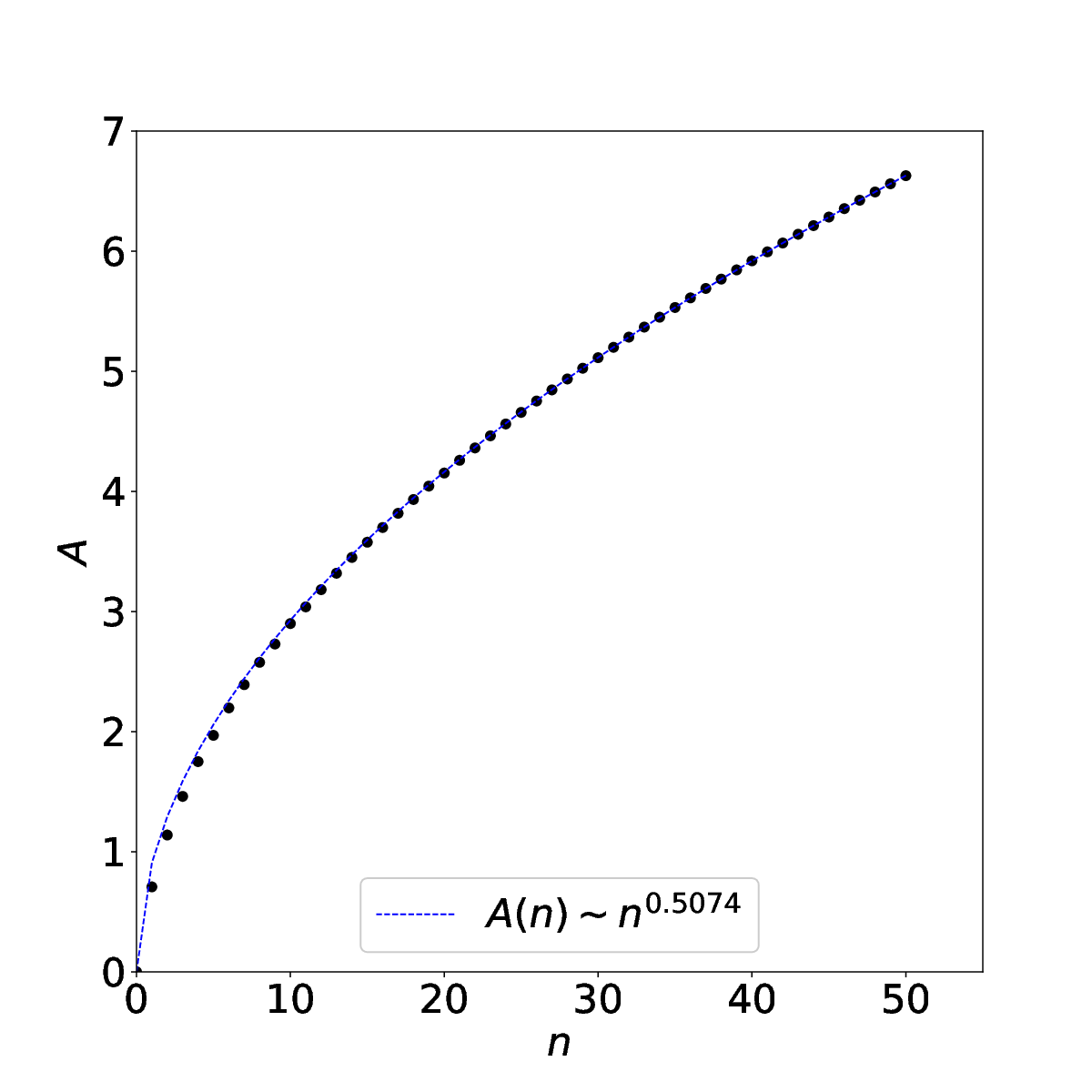
Computing the average positions, we find that the best fit is given by , which is very consistent with the classical curves (see FIG. 2). The amplitude depends on the initial wave function and is exactly , in such way that as grows, the amplitude of the mean oscillations also grows. To be more precise, , according to FIG. 3. As a result, considering more initial states, more energy is available for the system. Therefore, the phase space volume increases linearly with , because the classical energy is given by . The phase space volume can be easily calculated, in dimensionless variables, by the ellipses area , where is the proportionality constant. Thence, thermal properties can be estimated from these results, for instance the classical internal energy . By the canonical ensemble, the partition function can be written as follows
| (10) |
assuming a continuum sum of states. The internal energy yields , in agreement with the equipartition theorem. Even whether we consider a discrete number of states for in the canonical ensemble , we have the same result. Indeed,
| (11) |
where, by taking and using the definition of , we have , as expected.
5.2 Constant force
Let us focus on the constant force case. Despite of its simplicity, this example can be used, for instance, to simulate a charged harmonic oscillator in a uniform external electric field, and the effect of a weak gravitational field as well. We set, without loss of generality, . We notice that the general solution for the mean positions is given by , as expected (see FIG. 5 ). The classical solution is exactly the same of the previous one, despite of the translation of the position and amplitude by the value of 0.7. For an arbitrary constant, we must have and . The mean trajectories reproduce such property. Furthermore, in contrast with null force case, now for the particles have non-static trajectories and oscillatory averages, since the initial positions are not distributed around the equilibrium point. However, the momentum remains the same, implying that the phase space is shifted in the direction.


5.3 Impulsive Force
The impulsive forces have a wide class of applications in quantum systems. As examples we can cite non-adiabatic transitions [40], optomechanics [41, 42] and prediction of Gaussian quantum systems [43]. In our simulations we consider a fast acting impulsive force, modeled by , were we set the values of and . The asymptotic initial and final states are just the quantum harmonic oscillator, studied in the previous case. The difference is that the force brings more energy to the system, exciting more eingenstates and changing each individual weight of the linear superposition. The effect of such perturbation can be viewed in FIG. 6. Before the force acts, we have the same trajectories than the unforced case, passing to present a different behavior close to the peak of the Gaussian at . For , for example, the trajectories that are initially static pass to oscillate after the force ceases. As the effect of this perturbation, the volume of the phase space increases.


The averages are illustrated in FIG. 7. For all considered values of , the initial and final states have a sinusoidal form with different amplitudes, increasing the mean energy of the ensemble. This can be best understood looking to the phase space. In all examples we start in a circle of specific radius and, when the force starts to become relevant we are rapidly induced into a larger radius orbit, remaining there after the force stops. As we also expect, the averages obey Eq. (9).
5.4 Sinusoidal force
Let us focus on the sinusoidal force , where is the dimensionless temporal variable and is the ratio between the frequency of the external force and the fundamental frequency , this is to say, . The values of for the high and low frequency cases are chosen as and , respectively, with an amplitude of . We anticipate that their averages obey, with high precision, the classical laws (see FIG. 8).


As in the classic case, when a vibrating system is excited by a force with the same frequency, which is equivalent to take , the quantum resonance is observed . This phenomenon has been intensively investigated in the literature, with many applications as we can see in atom optics [44], experimental quasi-momentum measurements [45], multichromophoric energy transfer [46], electric-dipole moment experiments [47], and nano-resonance [48]. We restrict ourselves to show and to asses the quantum phase spaces and trajectories only for . In order to avoid the interference from unwanted boundary effects in the results, we take and . The trajectories are presented in FIG. 9. From the phase space we can see a monotonic increase in energy, since the trajectories spiral outwards as time passes, always expanding the volume of the phase space. We observe a typical resonant phenomenon for the mean trajectories, where the amplitude grows linearly with (see FIG. 10) as the force acts.


5.5 Quantum Duffing oscillator and resonance
Let us consider the quantum Duffing oscillator modeled by the following Hamiltonian
| (12) |
which can be viewed as a driven anharmonic oscillator with defined as the ratio between the external force frequency and the natural frequency of the correspondent harmonic oscillator obtained by taking . This model corresponds to a particular case of the Duffing equation [49], which finds applications in classical and quantum systems such as stiffening springs, beam buckling, nonlinear electronic circuits, superconducting Josephson parametric amplifiers, and ionization waves in plasmas [50]. In order to compare the results with the resonant case in the previous subsection, we consider , , and for the quartic potential responsible for the anharmonicity we set as a small perturbation.


In this case, a non-trivial difference between the first and third momentum, and , emerges as a consequence of the nonlinear force, namely , as in FIG. 11. The difference makes the quantum result slightly different from the classical one. Even for a small perturbation constant, as the values of the coordinate become large, this difference also increases. This result is naturally expected since the Ehrenfest theorem corresponds to the classical analogue only for linear and constant forces. The Ehrenfest theorem in the form of Eqs. (5) and (6) is still valid, however it does not correspond to an exact classical solution, but an approximate one. Let us emphasize that the average of the trajectories shown in FIG. 11 are in good agreement with the classical solution, evidencing that, at small perturbations, the correspondence between the classical and quantum equations still holds. At the beginning, when is small, the quadratic potential prevails. As a result, the quantum trajectories are subject to a resonant force that increases the amplitude of the oscillations as time passes. This leads the trajectories far away from the origin, where the effects of the anharmonic potential start to become relevant. Instead of having a constantly increasing amplitude as in the previous subsection, we have a beat-like pattern, since there is only a slight difference between the external frequency and the fundamental frequency , where is a small correction due to the anharmonic perturbation.
We would like to point out that for more complicated potentials as Coulomb or Morse potential, among others, which can not be accurately described by polynomials, the Ehrenfest theorem remains valid and can be studied by this numerical approach. However, focusing in classical-quantum equivalence of the trajectories, we concentrated on small corrections of the quantum harmonic oscillator and linear response theory, since this equivalence is achieved exactly () or almost exactly () for these cases.
Conclusions
In this work we prove numerically that the Ehrenfest theorem is also valid in the Bohmian mechanics, even for a certain non-conservative system as the forced quantum harmonic oscillator and Duffing oscillator. Since our approach is quite simple and has a few number of derivatives, it allows us to investigate a wide class of quantum systems without compute and simulate non-linear partial differential equations such as Eqs. (2) and (3). This method possibly can be a simpler manner to achieve classical results with very small boundary effects, at least for simple geometries. We observe that, as we increase the number of states , the quantum trajectories become more and more different of the classical analogues, however the averages obeys a classical law given in terms of the convolution (9), and the amplitudes of the oscillations depend on the number of states in the initial conditions. For we obtain that and the classical energy linearly depends on as well as its classical phase space volume. Thence, we reproduce the equipartition theorem by taking as a coordinate. Additionally, we can raise a question about the correspondence principle, since in the resonant case in subsection 5.4, the quantum trajectories preserved the structure of the classical result without taking account their average, and curiously, their time evolution was preserved even for non-zero values of .
For the Duffing oscillator, the Ehrenfest theorem can provide a satisfactory result for small perturbations when we performed the trajectories average, becoming a good starting point to explore other types of nonlinear potentials, even in the cases where the quantum-classical equivalence is not satisfied. Therefore, we conclude that the numerical procedures presented here can be used to investigate other quantum models where high accuracy and precision are necessary, such as integrable systems exhibiting unstable orbits, chaotic behavior, and can be extended for two and three-dimensional systems. We also can explore the noise effects in the quantum trajectories after adding an external random force instead of a deterministic one.
Acknowledgments
We acknowledge fruitful remarks by W. B. de Lima and P. de Fabritiis, as well as partial financial support from Conselho Nacional de Desenvolvimento Científico e Tecnológico (CNPq).
Author contributions
All the authors are responsible for the concept, design, execution, and physical interpretation of the research.
Declaration of Competing interests
The authors declare no competing interests.
References
- [1] L. de Broglie, Interference and Corpuscular Light. Nature, 118, 441–442 (1926).
- [2] D. Bohm, A Suggested Interpretation of the Quantum Theory in Terms of "Hidden" Variables. I. Phys. Rev., 85, 166 (1952).
- [3] D. Bohm, A Suggested Interpretation of the Quantum Theory in Terms of "Hidden" Variables. II. Phys. Rev., 85, 180 (1952).
- [4] D. A. Wisniacki and E. R. Pujals, Motion of vortices implies chaos in Bohmian mechanics, EPL, 71, 159 (2005).
- [5] C. Efthymiopoulos and G. Contopoulos, Chaos in Bohmian quantum mechanics, J. Phys. A: Math. Gen., 39, 1819 (2006).
- [6] S. Dey and A. Fring, Bohmian quantum trajectories from coherent states,Phys. Rev. A, 88, 022116 (2013).
- [7] I. A. Ivanov et al, Quantum chaos in strong field ionization of hydrogen, J. Phys. B: At. Mol. Opt. Phys., 52 , 225002 (2019).
- [8] A. C. Tzemos and G. Contopoulos, Chaos and ergodicity in an entangled two-qubit Bohmian system, Phys. Scr., 95, 065225 (2020).
- [9] A. Drezet, Justifying Born’s Rule Using Deterministic Chaos, Decoherence, and the de Broglie–Bohm Quantum Theory, Entropy, 23(11), 1371 (2021).
- [10] A. C. Tzemos, G. Contopoulos, Bohmian quantum potential and chaos, Chaos, Solitons and Fractals, 160, 112151 (2022).
- [11] W. Li, Analyzing quantum synchronization through Bohmian trajectories, Phys. Rev. A, 106, 023512 (2022).
- [12] R. Tsekov et al, Relating quantum mechanics with hydrodynamic turbulence, EPL, 122, 40002 (2018).
- [13] M. Bonilla-Licea, D. Schuch, Quantum hydrodynamics with complex quantities, Physics Letters A, 392, 127171 (2021).
- [14] M. Bonilla-Licea, D. Schuch, M. B. Estrada, Diffusion Effect in Quantum Hydrodynamics, Axioms, 11(10), 552 (2022).
- [15] M. Bonilla-Licea, D. Schuch, Uncertainty Relations in the Madelung Picture, Entropy, 24(1), 20 (2022).
- [16] V. Frumkin, D. Darrow, J. W. M. Bush, and Ward Struyve, Real surreal trajectories in pilot-wave hydrodynamics, Phys. Rev. A, 106, L010203 (2022).
- [17] F. Avanzini and G. J. Moro, Quantum Stochastic Trajectories: The Fokker-Planck-Bohm Equation Driven by the Reduced Density Matrix, J. Phys. Chem. A , 122, 2751-2763 (2018).
- [18] S. Wei, S. Li, F. Guo, Y. Yang, and B. Wang, Dynamic stabilization of ionization for an atom irradiated by high-frequency laser pulses studied with the Bohmian-trajectory scheme, Phys. Rev. A, 87, 063418 (2013).
- [19] H. Z. Jooya, D. A. Telnov, and S. Chu, Exploration of the electron multiple recollision dynamics in intense laser fields with Bohmian trajectories, Phys. Rev. A, 93, 063405 (2013).
- [20] Y. Song, S. Li, X. Liu, F. Guo, and Yu-Jun Yang, Investigation of atomic radiative recombination processes by the Bohmian-mechanics method Phys. Rev. A 88, 053419 (2013).
- [21] R. Sawada, T. Sato, and K. L. Ishikawa, Analysis of strong-field enhanced ionization of molecules using Bohmian trajectories, Phys. Rev. A, 90, 023404 (2014).
- [22] W. Xie, M. Li, Y. Zhou, and P. Lu, Interpreting attoclock experiments from the perspective of Bohmian trajectories Phys. Rev. A, 105, 013119 (2022).
- [23] B. Braverman and C. Simon, Proposal to Observe the Nonlocality of Bohmian Trajectories with Entangled Photons, Phys. Rev. Lett., 110, 060406 (2013).
- [24] A. C. Tzemos and G. Contopoulos, Ergodicity and Born’s rule in an entangled two-qubit Bohmian system, Phys. Rev. E, 102, 042205 (2020).
- [25] A.C. Tzemos, G. Contopoulos, Chaos and ergodicity in entangled non-ideal Bohmian qubits, Chaos, Solitons and Fractals, 156,111827 (2022).
- [26] O. V. Prezhdo and C. Brooksby, Quantum Backreaction through the Bohmian Particle, Phys. Rev. Lett., 86, 3215 (2001).
- [27] W. S. Santana et al, Evaluating Bohm’s quantum force in the scattering process by a classical potential, Eur. J. Phys., 42, 025406 (2021).
- [28] N. Pinto-Neto, The de Broglie-Bohm Quantum Theory and Its Applications to Quantum Cosmology,Universe, 7, 134 (2021).
- [29] N. Pinto-Neto Bouncing Quantum Cosmology, Universe, 241 (7), 110 (2021).
- [30] P. Ehrenfest, Bemerkung über die angenäherte Gültigkeit der klassischen Mechanik innerhalb der Quantenmechanik , Zeitschrift für Physik, 45 (7–8), 455–45 (1927).
- [31] V. Alonso, S. De Vincenzo, L. González-Díaz, Ehrenfest’s theorem and Bohm’s quantum potential in a “one-dimensional box”, Phys. Lett. A, 287, 23-30 (2001).
- [32] A. Valentini, Signal-locality, uncertainty, and the subquantum H-theorem. I, Physics Letters A, 156(1–2),5-11 (1991).
- [33] P. R. Holland, The quantum theory of motion: An Account of the de Broglie-Bohm Interpretation of Quantum Mechanics, Cambridge University Press, Cambridge, (1993).
- [34] S. De Vincenzo, On time derivatives for and : formal 1D calculations, Rev. Bras. Ensino Fís., 35 (2), 2308 (2013).
- [35] J. Wu, B. B. Augstein, and C. F. de Morisson Faria, Bohmian-trajectory analysis of high-order-harmonic generation: Ensemble averages, nonlocality, and quantitative aspects, Phys. Rev. A, 88, 063416 (2013).
- [36] E.N. Sarmin, L.A. Chudov, On the stability of the numerical integration of systems of ordinary differential equations arising in the use of the straight line method, USSR Computational Mathematics and Mathematical Physics, 3 (6), 1537–1543 (1963).
- [37] P. W. C. Northrop, P. A. Ramachandran, W. E. Schiesser, and V. R. Subramanian , A Robust False Transient Method of Lines for Elliptic Partial Differential Equations, Chem. Eng. Sci., 90, pp. 32–39 (2013).
- [38] S.Hamdi, W. E. Schiesser G. W. Griffiths , "Method of lines", Scholarpedia, 2 (7), 2859 (2017).
- [39] P.A. Zegeling, Tensor-product adaptive grids based on coordinate transformations, Journal of Computational and Applied Mathematics, 166, 343-360 (2004).
- [40] D. F. Coker and L. Xiao, Methods for molecular dynamics with nonadiabatic transitions, J. Chem. Phys., 102, 496 (1995).
- [41] D. Vitali, S. Mancini, and P. Tombesi, Optomechanical scheme for the detection of weak impulsive forces, Phys. Rev. A, 64, 051401(R) (2001).
- [42] J. S. Bennett and W. P. Bowen, New J. Phys., 20, 113016 (2018).
- [43] Z. Huang and M. Sarovar, Smoothing of Gaussian quantum dynamics for force detection, Phys. Rev. A, 97, 042106 (2018).
- [44] S. Fishman, I. Guarneri, and L. Rebuzzini, Stable Quantum Resonances in Atom Optics Phys. Rev. Lett., 89, 084101 (2002).
- [45] I. Dana, V. Ramareddy, I. Talukdar, and G. S. Summy, Experimental Realization of Quantum-Resonance Ratchets at Arbitrary Quasimomenta, Phys. Rev. Lett., 100, 024103 (2008).
- [46] S. Duque, P. Brumer, and L. A. Pachón, Classical Approach to Multichromophoric Resonance Energy Transfer, Phys. Rev. Lett., 115, 110402 (2015).
- [47] A.J. Silenko, General classical and quantum-mechanical description of magnetic resonance: an application to electric-dipole-moment experiments, Eur. Phys. J. C , 77, 341 (2017).
- [48] V.V. Egorov, Quantum–Classical Mechanics: Nano-Resonance in Polymethine Dyes, Mathematics, 10, 1443 (2022).
- [49] G. Duffing, Erzwungene Schwingung bei veränderlicher Eigenfrequenz und ihre technische Bedeutung, Vieweg, Braunschweig (1918).
- [50] H. J. Korsch, H. Jodl and T. Hartmann, Chaos: A Program Collection for the PC, Springer, Berlin (2008).