When, where, and how many planets end up in first-order resonances?2022When, where, and how many planets end up in first-order resonances?--B.2

As most observed transiting planets are located within $\sim$1 au of their host star, we will describe the possible structures of the inner disc. We assume that the gas surface density always follows a power-law distribution:

$$\Sigma(r)=\Sigma_{\mathrm{1au}}\left(\frac{r}{1\,\mathrm{au}}\right)^{s},$$

(2)

where $\Sigma_{\mathrm{1au}}$ is the gas surface density at $1\,\mathrm{au}$ and $s$ is its slope. The gas aspect ratio also follows a power-law distribution:

$$h(r)=h_{\mathrm{1au}}\left(\frac{r}{1\,\mathrm{au}}\right)^{q}$$

(3)

where $h_{\mathrm{1au}}$ is the gas aspect ratio at $1\,\mathrm{au}$ and $q$ is its slope. Different assumptions about the disc structure, e.g., heating mechanisms, result in distinct values of $s$, $q$, $\Sigma_{\mathrm{1au}}$, and $h_{\mathrm{1au}}$. Typically, the inner disc is optically thick and the main heating energy comes from viscous dissipation (Ruden & Lin 1986), while the outer disc is optically thin and stellar irradiation mainly heat the disc onto its surface layer (Chiang & Goldreich 1997).

For discs dominated by stellar radiation, we make use of the disc structure from Liu et al. 2019. The gas surface density is:

$$\Sigma_{\mathrm{g,irr}}=250\left(\frac{\dot{M}_{g}}{10^{-8}M_{\odot}/\mathrm{yr}}\right)\left(\frac{M_{\star}}{M_{\odot}}\right)^{\frac{9}{14}}\left(\frac{L_{\star}}{L_{\odot}}\right)^{-\frac{2}{7}}\left(\frac{r}{\mathrm{au}}\right)^{-\frac{15}{14}}\mathrm{g\,cm}^{-2}$$

(4)

where $\dot{M}_{g}$ is stellar accretion rate and $L_{\star}$ is the star luminosity. The aspect ratio is:

$\displaystyle h_{\mathrm{g,irr}}=$

$\displaystyle 0.0245\left(\frac{M_{\star}}{1M_{\odot}}\right)^{-4/7}\left(\frac{L_{\star}}{1L_{\odot}}\right)^{1/7}\left(\frac{r}{1\,\mathrm{au}}\right)^{2/7}.$

(5)

For stars of mass between $0.43M_{\odot}$ and $2M_{\odot}$, which covers most of our star sample, the mass-luminosity relation is well represented by ${L_{\star}}/{L_{\odot}}=\left({M_{\star}}/{M_{\odot}}\right)^{4}$ (Duric 2004). Therefore, the disc aspect ratio simplifies to:

$$h_{\mathrm{g,irr}}=0.0245\left(\frac{r}{1\,\mathrm{au}}\right)^{2/7}$$

(6)

independent of stellar mass.

If the inner disc is dominated by viscous heating, its temperature structure is highly related to the viscous accretion rate and opacity. Following Liu et al. 2019, $s$ and $q$ are taken to be $-3/8$ and $-1/16$, while $\Sigma_{\mathrm{1au}}$ and $h_{\mathrm{1au}}$ are not specified.

In the Type I migration regime, planet migration is the result of a net torque $\Gamma_{\mathrm{net}}$ consisting of the Lindblad (Ward 1986; Ward 1997), corotation (Goldreich & Tremaine 1979; Ward 1992) and thermal torques (Benítez-Llambay et al. 2015; Masset 2017; Guilera et al. 2019; Guilera et al. 2021), etc. Usually, the net torque is negative and the planet migrates inward. In the Type I limit the migration speed is proportional to disc mass and planet mass. In the limit of a locally isothermal disc, which implies that temperature is a function of radius only, $T(r)$, the type I migration time-scale for the $i$-th planet at distance $r_{i}$ is:

$$\tau_{a_{i}}=\frac{L_{i}}{\Gamma_{\mathrm{net}}}=\frac{\gamma_{I}\tau_{w_{i}}}{h(r_{i})^{2}},$$

(7)

where $L_{i}$ is the angular momentum of the planet, $\gamma_{I}=2.7-1.1s$ (Tanaka et al. 2002) is the Type I migration prefactor (D’Angelo & Lubow 2010), and $h(r_{i})$ is the disc gas aspect ratio at $r_{i}$. The characteristic time of the orbital evolution (Tanaka & Ward 2004) is:

$$\tau_{w_{i}}=\frac{1}{\mu_{i}}\frac{M_{\star}}{\Sigma(r_{i})r_{i}^{2}}\frac{h(r_{i})^{4}}{\Omega_{K}(r_{i})},$$

(8)

where $\mu_{i}$ is the mass ratio of the $i$-th planet over its host star and $\Omega_{K}(r_{i})=\sqrt{GM_{\star}/r_{i}^{3}}$ is the Keplerian angular velocity at distance $r_{i}$. The eccentricity damping rate is proportional to the local surface density and planet mass. It is given by:

$$\tau_{e_{i}}=\frac{C_{e}\tau_{w_{i}}}{0.78}=\frac{C_{e}}{0.78\gamma_{I}}h^{2}\tau_{a},$$

(9)

where $C_{e}$ stands for eccentricity damping efficiency. Although Cresswell & Nelson 2008 gives $C_{e}\approx 1$, lower values are needed in other studies to reproduce specific systems. TRAPPIST-1 planets demand $C_{e}\approx 0.1$ (Huang & Ormel 2022) and K2-24 requires $C_{e}\approx 0.28$ (Teyssandier & Libert 2020). A recently discovered ${\sim}100\,\mathrm{Myr}$ old exoplanet system TOI-1136, on the other hand, suggest $C_{e}\sim 10$ (Dai et al. 2022). We are therefore agnostic about the value of $C_{e}$, which value we intend to constrain through our MCMC fitting.

Resonance trapping is a natural outcome of convergent disc migration and eccentricity damping, especially for first-order resonances $(j+1){:}j$. When two planets are in first-order resonance, their eccentricities and period ratio librate around their equilibrium values. Such equilibrium has been studied by Goldreich & Schlichting 2014 and Terquem & Papaloizou 2019. They both give the equilibrium eccentricity (the eccentricity where tidal damping equals resonant excitation) of the inner planet:

$$e_{\mathrm{1,eq}}^{2}=\frac{\tau_{e_{1}}/\tau_{a_{2}}-\tau_{e_{1}}/\tau_{a_{1}}}{2(j+1)\left(1+\frac{j}{j+1}\frac{\mu_{1}}{\alpha\mu_{2}}\right)\left[1+\frac{\mu_{1}}{\alpha\mu_{2}}\left(\frac{j}{j+1}\right)^{2}\left(\frac{f_{2}^{\prime}}{f1}\right)^{2}\frac{\tau_{e_{1}}}{\tau_{e_{2}}}\right]}$$

(10)

where $\alpha$ is ratio of the inner-to-outer semi-major axis . Here, and in the following, the subscription ’1’ stands for the inner planet and ’2’ for the outer planet. The relationship between the eccentricities of the inner and outer planets is:

$$\frac{e_{2}^{2}}{e_{1}^{2}}=\left(\frac{\mu_{1}}{\alpha\mu_{2}}\frac{j}{j+1}\frac{f_{2}^{\prime}}{f_{1}}\right)^{2},$$

(11)

where $f_{1}$ and $f_{2}^{\prime}$ are coefficients tabulated in Terquem & Papaloizou 2019. The equilibrium value for the offset from exact resonance is:

$$\Delta_{\mathrm{eq}}=-f_{2}^{\prime}\mu_{1}\frac{1}{j}\frac{1}{e_{\mathrm{2,eq}}}.$$

(12)

At this distance, the resonance repulsion equals the Type-I inward migration.

In order to calculate the period ratios for planets in resonance, we need to know what their equilibrium eccentricities are. This calculation can be done only after the values of ${\tau_{e_{1}}}/{\tau_{e_{2}}}$, ${\tau_{e_{1}}}/{\tau_{a_{2}}}$ and ${\tau_{e_{1}}}/{\tau_{a_{1}}}$ are known. Combining the disc model and migration model, we have

$$\frac{\tau_{e_{1}}}{\tau_{e_{2}}}=\frac{\mu_{2}}{\mu_{1}}\left(\frac{r_{1}}{r_{2}}\right)^{4q-s-0.5}$$

(13)

and

$$\frac{\tau_{e_{1}}}{\tau_{a_{2}}}=\frac{\tau_{e_{2}}}{\tau_{a_{2}}}\frac{\tau_{e_{1}}}{\tau_{e_{2}}}=\frac{C_{e}h(r_{2})^{2}}{0.78\gamma_{I}}\frac{\mu_{2}}{\mu_{1}}\left(\frac{r_{1}}{r_{2}}\right)^{4q-s-0.5}$$

(14)

where $s$ and $q$ are gas surface density and aspect ratio gradient.

For the eccentricity-to-semi-major axis damping of the inner planet, we distinguish it between two cases:

1. 1.

   Migrating pair. If resonances are formed during migration and the ambient disc disperses before the planet pairs reach a migration barrier, planet migration and eccentricity damping follow Eq. (7) and Eq. (9). Therefore,

   $$\frac{\tau_{e_{1}}}{\tau_{a_{1}}}=\frac{C_{e}h(r_{1})^{2}}{0.78\gamma_{I}}$$

   (15)

   It requires that the outer planet migrates faster than the inner planet to guarantee convergent migration.

2. 2.

   Braking pair. On the other hand, if resonances are formed before/after the inner planet’s migration is halted by a barrier (could be disc inner edge or the radius where reverse migration occurs), there is no net torque on the two planets. Angular momentum conservation gives $\tau_{a_{1}}/\tau_{a_{2}}=-\sqrt{\mu_{1}r_{1}/\mu_{2}r_{2}}$. Hence,

   	$\displaystyle\frac{\tau_{e_{1}}}{\tau_{a_{1}}}$	$\displaystyle=-\frac{C_{e}h(r_{2})^{2}}{0.78\gamma_{I}}\left(\frac{\mu_{2}}{\mu_{1}}\right)^{\frac{3}{2}}\left(\frac{r_{1}}{r_{2}}\right)^{4q-s-1}$		(16)
   		$\displaystyle=-\frac{C_{e}h(r_{1})^{2}}{0.78\gamma_{I}}\left(\frac{\mu_{2}}{\mu_{1}}\right)^{\frac{3}{2}}\left(\frac{r_{1}}{r_{2}}\right)^{2q-s-1}$

For the outer planet ${\tau_{e_{2}}}/{\tau_{a_{2}}}={C_{e}h(r_{2})^{2}}/{0.78\gamma_{I}}$ is always true. It is also apparent that the resonant equilibrium does not depend on disc mass ($\Sigma_{\mathrm{1au}}$) but on power law indices and aspect ratio ($s$, $q$, and $h_{\mathrm{1au}}$).

Planets’ masses are also needed to calculate the equilibrium period ratios in resonance. However, most transiting planets have poorly constrained masses compared to their radii.

If the planet mass is not yet constrained from e.g., Transit Timing Variation (Agol et al. 2005, TTV) or Radial Velocity (RV), we then obtain the planet mass using a mass-radius relation. The planet sample for fitting the mass-radius relation is based on the data of transiting planets from the NASA Exoplanet Archive¹¹ 1 https://exoplanetarchive.ipac.caltech.edu. Planets with masses lower than $200M_{\earth}$, radii smaller than $20R_{\earth}$, or periods longer than $5$ days (see Sect. 4.1) are selected while planets with periods shorter than $5$ days are excluded.

Our fitting approach is identical to Ramos et al. 2017. They use a broken power law expression, which fits two different power law relations for larger bodies ($R>R_{\mathrm{crit}}$) and smaller bodies ($R<R_{\mathrm{crit}}$).

$$\log_{10}\left(\frac{\overline{M}_{i}}{M_{\earth}}\right)=\left\{\begin{array}[]{ll}a+b\log_{10}\left(\frac{R_{i}}{R_{\earth}}\right)&\text{if }R_{i}\leq R_{\mathrm{crit}}\\ c+d\log_{10}\left(\frac{R_{i}}{R_{\earth}}\right)&\text{if }R_{i}>R_{\mathrm{crit}}\end{array}\right.$$

(17)

where $M_{i}$ and $R_{i}$ is the mass and radius of the $i$-th planet. We make use of the Maximum Likelihood Estimator (MLE) to maximize a Gaussian likelihood centered at Eq. (17). The critical radius $R_{\mathrm{crit}}$ is also fitted. It estimates that: $a=0.69$, $b=0.78$, $c=0.11$, $d=1.7$, $R_{\mathrm{crit}}=4.23R_{\earth}$ and the corresponding dispersion $\sigma_{m}=0.374$. The best-fitting relation is shown in Fig. 1 in comparison with the relation fitted by Ramos et al. 2017. They do not differ significantly. The estimated value for $R_{\mathrm{crit}}$ is consistent with Teske et al. 2021 who suggest a single power law relation for planets with $R<3.25R_{\oplus}$.

Equation (17) allows us to calculate the planet mass and therefore the resonance offset (Eq. (12)). Moreover, the log-normal dispersion in planet mass enables us to check our model consistency. The reason is that any uncertainty in the mass, will propagate, through Eq. (10) and Eq. (12). Therefore, we expect that the obtained value for $\sigma_{\Delta}$ from MCMC fitting is similar to, or exceeds, $\sigma_{m}$.

The log-normal dispersion in planet mass significantly simplifies our analysis. There are arguably more sophisticated forms of M-R relationships, e.g., the one given by Wolfgang et al. 2016 and improved by Teske et al. 2021. However, they assume planet mass follows a normal dispersion instead of a log-normal. In that case, the resulting $\Delta$ would follow a complicated form of the ratio distribution²² 2 If variables $X$ and $Y$ follow a dependent (independent) normal distribution with nonzero mean values, the new variable $Z=X/Y$ follows correlated (uncorrelated) non-central normal ratio distribution (Hinkley 1969; Hayya et al. 1975)..

We define the posterior distribution as: $p(\bm{\theta}|\Delta_{\mathrm{obs},k},\bm{X}_{k})=p(\Delta_{\mathrm{obs},k}|\bm{\theta},\bm{X}_{k})p(\bm{\theta}|\bm{X}_{\mathrm{obs},k}).$ If the disc structure is not specified (without knowing the specific values of $s$, $q$ in Eq. (2) and Eq. (3)), the unknown model parameters are $\bm{\theta}=(\log_{10}(C_{e}h_{\mathrm{1au}}^{2}),\sigma_{\Delta},s,q)$ and the known parameters $\bm{X}_{k}=(M_{\star},M_{1},M_{2},r_{1},r_{2},j)$. The index $k$ indicates the $k$-th planet pair. If a disc structure is specified, the unknown model parameters are $\bm{\theta}=(\log_{10}C_{e},\sigma_{\Delta})$ for the irradiation disc and $\bm{\theta}=(\log_{10}(C_{e}h_{\mathrm{1au}}^{2}),\sigma_{\Delta})$ for the viscous disc, and the known parameters are $\bm{X}_{k}=(M_{\star},M_{1},M_{2},r_{1},r_{2},j,h_{\mathrm{1au}},s,q)$. We assume that the prior $p(\bm{\theta}|\bm{X}_{k})$ follows a uniform distribution (Table 1). The resonance index $j$ is regarded as one of the known parameters such that we can analyse all pairs at once.

As mentioned, resonance trapping naturally results from convergent migration: either two planets get trapped into resonance during migration (both inward) with the outer planet migrating faster than the inner one, or the inner planet reaches a migration barrier with the outer planet arriving at a later time. Following the discussion in Sect. 2.4, we assume that the period ratio of a planet pair that is in resonance obeys a log-normal distribution $\log_{10}\Delta\sim\mathcal{N}(\log_{10}\Delta_{\mathrm{m/s}}(\bm{\theta},\bm{X}_{k}),\sigma_{\Delta}^{2})$:

		$\displaystyle p_{\mathrm{res,m/s}}(\Delta|\bm{\theta},\bm{X}_{k})d\log_{10}{\Delta}$		(18)
		$\displaystyle=\frac{1}{\sqrt{2\pi\sigma_{\Delta}^{2}}}\exp{\left[-\frac{[\log_{10}\Delta-\log_{10}\Delta_{\mathrm{m/s}}(\bm{\theta},\bm{X}_{k})]^{2}}{2\sigma_{\Delta}^{2}}\right]}d\log_{10}{\Delta},$

where $\Delta_{\mathrm{m/s}}$ indicates the resonance commensurability calculated by Eq. (12). The resonance offset $\Delta_{\mathrm{m}}$ indicates the value calculated for Migrating pairs using Eq. (15), while $\Delta_{\mathrm{s}}$ is for Braking pairs and is calculated using Eq. (16).

In the Type I migration regime, if the inner planet is more massive (migrates faster), convergent migration can only occur when the inner planet has reached the migration barrier. On the other hand, if the inner planet’s migration is slower than the outer, migration is always convergent. In that case, trapping can occur when both planets migrate inward or when the inner planet has reached the migration barrier. For ease of the likelihood calculation, we further divide the resonant planet pairs into three categories:

1. Group 1:

   The inner planet migrated slower ($\tau_{a_{1}}>\tau_{a_{2}}$) and it did not reach a migration barrier ($N_{1}$);

2. Group 2:

   The inner planet migrated slower ($\tau_{a_{1}}>\tau_{a_{2}}$) and it reached a migration barrier ($N_{2}$);

3. Group 3:

   The inner planets migrated faster ($\tau_{a_{1}}\leq\tau_{a_{2}}$) and it reached a migration barrier ($N_{3}$).

$N_{1}$, $N_{2}$ and $N_{3}$ represent the number of resonant planet pairs corresponding to each type of resonance. In addition, $N_{4}$ ($N_{5}$) represents the number of pairs that are not in resonance with the inner planet migrating faster (slower) than the outer planet. We provide a sketch to explain the five classes in Fig. 2.

If the inner planets migrate faster ($\tau_{a_{1}}\leq\tau_{a_{2}}$), those pairs in resonance must be Braking pairs. However, if the inner planets migrate slower, they could either be Migrating pairs or Braking pairs. The $\log_{10}\Delta$ distribution of planets in resonance is therefore (hereafter, $p_{\mathrm{res}}(\Delta)$ represents $p_{\mathrm{res}}(\Delta_{\mathrm{obs}}|\bm{\theta},\bm{X}_{k})$, etc):

$\displaystyle p_{\mathrm{res}}(\Delta)$

$\displaystyle=\left\{\begin{array}[]{ll}p_{\mathrm{res,s}}(\Delta)&\mathrm{if}\,\tau_{a_{1}}\leq\tau_{a_{2}},\\ \left[p_{\mathrm{res,s}}(\Delta)+p_{\mathrm{res,m}}(\Delta)\right]&\mathrm{if}\,\tau_{a_{1}}>\tau_{a_{2}}.\end{array}\right.$

(19)

The period ratio of planet pairs that are not in resonance is assumed to follow a uniform distribution:

$$p_{\mathrm{n-res}}(\Delta)d\log_{10}{\Delta}=\frac{(\ln{10})\Delta}{\Delta_{\mathrm{max}}}d\log_{10}{\Delta}$$

(20)

where $\Delta_{\mathrm{max}}$ is the value above which a planet pair with $\Delta_{\mathrm{obs}}$ is not considered in resonance. We use $\Delta_{\mathrm{max}}=(3j+2)/(3j-1)-(j+1)/j$ which is the distance from the first order $(j+1):j$ resonance to its closest external 3rd order $(3j+2):(3j-1)$ resonance.

Finally, the total log-likelihood is written as:

$\displaystyle\ln\mathcal{L}=\sum_{k=1}^{N_{\mathrm{pairs}}}\ln\left[p_{\mathrm{res}}(\Delta_{\mathrm{obs},k})+p_{\mathrm{n-res}}(\Delta_{\mathrm{obs},k})\right],$

(21)

where $N_{\mathrm{pairs}}$ is the number of planet pairs in our sample.

In the restricted three-body problem, the outer planet is on a fixed circular orbit. The inner planet moves outward and its semi-major axis and eccentricity are damped on time-scales of $\tau_{a}$ and $\tau_{e}$, respectively. Lagrange’s planetary equation for the mean motion ($n$) then reads:

$$\dot{n}_{1}=-3j\alpha f_{1}\mu_{2}e_{1}n_{1}^{2}\sin{\phi_{1}}-\frac{3n_{1}}{2\tau_{a}}+\frac{pe_{1}^{2}n_{1}}{\tau_{e}},$$

(22)

where $\alpha=a_{1}/a_{2}$, $\phi_{1}$, $e_{1}$ and $f_{1}$ are the semi-major axis ratio, resonance angle, the eccentricity of the inner planet, and $f_{1}$ is a numerical factor that depends on the resonance index $j$ (Murray & Dermott 1999; Terquem & Papaloizou 2019). By definition, $p=3$ holds when the eccentricity damping operates at constant angular momentum (Teyssandier & Terquem 2014). Lagrange’s planetary equation for eccentricity is:

$$\dot{e}_{1}=-\alpha f_{1}\mu_{2}n_{1}\sin{\phi_{1}}-\frac{e_{1}}{\tau_{e_{1}}},$$

(23)

When two planets are in resonance, the values of different orbital properties e.g., $e_{1}$, $\alpha$ and $\phi_{1}$ librate around their equilibrium values. The equilibrium eccentricity (Goldreich & Schlichting 2014; Terquem & Papaloizou 2019) is derived by putting $\dot{e}=\dot{a}=0$ and eliminating $\sin{\phi_{1}}$ in Eq. (22) and Eq. (23):

$$e_{\mathrm{1,eq}}=\sqrt{\frac{\tau_{e_{1}}}{2(j+1)\tau_{a_{1}}}}.$$

(24)

By inserting the equilibrium eccentricity $e_{\mathrm{1,eq}}$ and $\alpha_{\mathrm{eq}}\approx[j/(j+1)]^{2/3}$ into Eq. (23), $\sin\phi_{1}$ follows:

$$\sin\phi_{1,\mathrm{eq}}=-\frac{1}{\alpha f_{1}\mu_{2}n_{1}}\sqrt{\frac{1}{2(j+1)\tau_{e_{1}}\tau_{a_{1}}}}$$

(25)

Naturally, its absolute value cannot exceed 1. Otherwise, for $|\sin\phi_{1}|>1$, no steady state exists and the planets will cross the resonance. Combining, $\dot{e}_{1}=0$, Eq. (23) and Eq. (24) we can write the resonance trapping condition:

$$\tau_{a_{1}}\tau_{e_{1}}\geq\frac{1}{2(j+1)(\alpha f_{1}\mu_{2}n_{1})^{2}}.$$

(26)

The classical theory about the resonance trapping criterion is that the time for the planet to migrate across the libration width is shorter than the libration time-scale (Ogihara & Kobayashi 2013; Batygin 2015). For comparison, we also provide the criterion derived from the classical pendulum model (Murray & Dermott 1999; Ogihara & Kobayashi 2013; Huang & Ormel 2022):

$$\tau_{a_{1}}\tau_{e_{1}}\geq\frac{\pi(j+1)}{4(\alpha f_{1}\mu_{2}n_{1})^{2}}.$$

(27)

Compared to Eq. (27), the new criterion (Eq. (26)) has the same dependence on planet-to-star mass ratio $\mu_{2}$ and the orbital frequency $n_{1}$ but differs regarding the resonance index $j$.

We compare the new resonance trapping criterion above against the numerical simulation. The fiducial accelerations accounting for migration and eccentricity of planets in the simulations are expressed by:

$$\bm{a}_{\mathrm{m}}=-\frac{\bm{v}}{2\tau_{a}},$$

(28)

$$\bm{a}_{\mathrm{e}}=-2\frac{(\bm{v}\cdot\bm{r})\bm{r}}{2r^{2}\tau_{e}}$$

(29)

(Papaloizou & Larwood 2000; Cresswell & Nelson 2006; Cresswell & Nelson 2008). We make use of the WHfast integrator of the open-source N-body code REBOUND (Rein 2012). The migration and eccentricity damping on planets are implemented through REBOUNDx (Tamayo et al. 2020).

We fix the outer planet on a circular orbit at $[(j+1)/j]^{2/3}$ au. The inner planet starts to migrate outward at $0.8$ au on a time-scale of $\tau_{a}$. Its eccentricity is damped on a time-scale of $\tau_{e}$. The planet mass is fixed at $10\,M_{\oplus}$ and the host mass is $1\,M_{\odot}$. We vary two parameters in the simulation: $\tau_{a}$ from $10^{4}$ yr (fast migration) to $10^{7}$ yr (slow migration), and $\tau_{a}/\tau_{e}$ ranging from $10^{1}$ (inefficient eccentricity damping) to $10^{4}$ (efficient eccentricity damping). Each parameter is sampled by 100 grid points evenly distributed in log-space. In order to capture the probabilistic behavior of resonance trapping, we run five simulations for each point in the $\tau_{a}/\tau_{e}$--$\tau_{a}$ parameter space, where we evenly sample the initial longitude of the inner planet.

We conduct simulations for $j=1$ (2:1 resonance) and $j=2$ (3:2 resonance). We run the simulation until $t=\tau_{a}$, but we take a snapshot at $t=0.2\tau_{a}$. If the period ratio $P_{2}/P_{1}$ decreases below $(j+1)/j$, we classify the simulation outcome as a resonance crossing. The results are shown in Fig. 3 and Fig. 4 for $j=1$ and $j=2$ respectively. Resonance crossing cases are in white and resonance trapping cases are in green. The red dashed line indicates the boundary below which the trapping solution becomes overstable,

$$\left(\frac{\tau_{a}}{\tau_{e}}\right)_{\mathrm{overstable}}=\frac{1}{8(j+1)}\left(-\frac{3j^{2}}{\alpha f_{1}\mu_{2}}\right)^{2/3}$$

(30)

(Goldreich & Schlichting 2014), which evaluates to $\tau_{a}/\tau_{e}\approx$170 for $\mu_{2}=3\times 10^{-5}$, both for $j=1$ and 2. Above this line, all systems are either trapped in resonance or not. The top-right corner indicates the parameter space where the two planets both get captured and permanently stay in resonance and the top-left indicates resonance crossing. Below this line, some systems are still evolving and resonance trapping is only temporary.

We indicate the trapping criterion derived from the pendulum model in blue and the improved trapping criterion (Eq. (26)) with the orange line. From Fig. 3 and 4 it is clear that the pendulum model criterion for resonance trapping (blue line) fails to quantitatively match the numerical simulations. Our new criterion (orange line), however, fits the simulations perfectly. The equilibrium value of $\sin\phi_{\mathrm{1}}$ for the simulation snapshots is calculated by averaging its value over a time span of $0.1\tau_{a}$ before and after the snapshot time, e.g., $0.1-0.3\tau_{a}$ for the snapshot at $t=0.2\tau_{a}$. The values of $\sin\phi_{\mathrm{1,eq}}$ is indicated by grey solid lines (contour) in Fig. 3 and 4. $\sin\phi_{\mathrm{1,eq}}$ increases as getting closer to the orange line, which is also expected by Eq. (25). The picture of resonance trapping/crossing over the entire parameter space of the migration time-scale and eccentricity damping time-scale has now been clarified. Migration plays a role in exciting the planet’s eccentricity, while eccentricity damping reduces it. On one hand, if a planet pair is in resonance, the eccentricity damping balances its excitation and finally librates near the equilibrium value. If the migration speed is so fast that there is no steady state solution for the resonance angle $\phi_{\mathrm{1,eq}}$ (Eq. (26)), the resonance is crossed. Otherwise, resonance trapping is ensured. On the other hand, if eccentricity is excited to be high enough, planets can be captured into resonance, but only temporarily, because of the continuous increase of the resonance libration amplitude (Goldreich & Schlichting 2014, overstability, cf.). Although not evident from the figures presented, all simulations located in the large green corner above the red dashed line exhibit permanent libration of $\sin\phi_{\mathrm{1}}$, indicating that the planets are captured in resonance permanently. The amplitude of $\sin\phi_{\mathrm{1}}$ during libration increases as the ratio $\tau_{a}/\tau_{e}$ decreases, and approaches the red dashed line denoting overstability in Fig. 3 and 4. The green region situated below the red dashed line represents simulations in which planets are temporarily captured in resonance, with their amplitude of $\sin\phi_{\mathrm{1}}$ increasing over time and circulating at the end of the simulation. In conclusion, both efficient eccentricity damping ($\tau_{a}/\tau_{e}$ is high) and slow migration are required for permanent resonance trapping.

Our sample selection and all analysis are based on the NASA Exoplanet Archive. Our attention is drawn to planets detected through transits and TTV. As shown in Sect. 2.3, we need planets’ masses to calculate the equilibrium eccentricities and period ratios in resonance. If only the radius is available, the M-R relationship described in Sect. 2.4 is used to calculate the masses of those transiting planets. Additionally, the semi-major axes and stellar masses are extracted.

We do not consider short-period planets in our sample. We take this simple step to reduce the effects of both photo-evaporation and stellar tides on the M-R relationship. First, photo-evaporation can alter the M-R relationship for planets with low-density atmospheres on time-scale of 1 Gyr (Fulton & Petigura 2018). It is believed to have triggered the so-called ‘radius gap’ (Fulton et al. 2017). When planets get closer to their host stars, this effect is more obvious (Fulton & Petigura 2018). Second, stellar tides alter close-in planets’ orbital properties (Lithwick & Wu 2012; Batygin & Morbidelli 2013; Charalambous et al. 2018; Papaloizou et al. 2018) and blur the information of the planets inherited from their protoplanet disc. Both mechanism are very sensitive to planets’ semi-major axes. Excluding the planets with a cutoff period shorter than 5 days, though crude, can suppress the interference from stellar tides (Choksi & Chiang 2020) and photo-evaporation (Fulton & Petigura 2018) on our sample.

We display the planet mass versus their host mass in Fig. 5. The average planet mass is $10M_{\oplus}$ and the average stellar mass is $1\,M_{\odot}$. The planets’ and stars’ mass uncertainties are indicated by error bars. If the planet mass is inferred from the M-R relation, the log-normal standard deviation is then $\sigma_{m}=0.374$ (Eq. (17)). The migration speed of low-mass planets in the proto-planetary disc scales linearly with planet mass, as dictated by the Type I migration limit. As planets become massive enough to perturb their surrounding disc, their migration gradually switches to Type II (Kanagawa et al. 2018; Pichierri et al. 2022). We set the boundary between two types of migration as $\mu_{\mathrm{trans}}=10^{-4}$. Since our interests focus on Type I migration only planets with $\mu<\mu_{\mathrm{trans}}$ are included in our sample.

Finally, the sample size is reduced to 371 and the period ratios for all planet pairs are given by Fig. 6. The selected planets come from systems with two and more planets, including those with resonance chains.

To calculate the resonance offset, the resonance number $j$ is required. There are excesses of systems (’peaks’) just wide of the integer period ratios, which is suggestive of resonances. We only consider first-order resonances: 2:1, 3:2, 4:3, and 5:4. We assume that planets with period ratios slightly larger than the integer ratios are potentially in resonance until the period ratio "hits" the third-order resonance, because the resonant interaction is weaker as they become further from exact commensurability. Planet pairs with period ratios larger than $(j+1)/j$ but smaller than $(3j+2)/(3j-1)$ are possibly in $(j+1)/j$ resonance. Here, $(3j+2)/(3j-1)$ is the location of the closest third-order resonance. The selection of a period ratio limit for identifying planets in 2:1 resonance may seem arbitrary, given that the period ratio can extend up to 2.5, where planet pairs are unlikely to be in resonance. However, a slightly smaller window for the 2:1 resonance would not affect our conclusions. Nonetheless, this choice is useful for identifying planets in 3:2, 4:3, and higher $j$ first-order resonances because planets located near these resonance locations are close to nearby higher-order resonances, and may therefore be more easily perturbed. The satisfied period ratio windows are highlighted in Fig. 10 (top panel) and the four lower panels zoom in on these four windows, for $j=$1, 2, 3, 4, where we instead show the distribution of the offset from resonance, $\Delta$. Planets out of the windows may still be in first-order resonance, but their fraction must be very low and it is not covered by our analysis. We ignore other first-order resonances and all higher-order resonances.

We use emcee (Foreman-Mackey et al. 2013) to perform the MCMC analysis. We implement three different models:

1. 1.

   General model. The disc structure is not specified and the MCMC is used to fit $\log_{10}(C_{e}h_{\mathrm{1au}}^{2})$, $\sigma_{\Delta}$, $s$, $q$.

2. 2.

   Irradiation model. Stellar irradiation is assumed to be the main heating source and the MCMC is used to fit $\log_{10}C_{e}$ and $\sigma_{\Delta}$.

3. 3.

   Viscous model. Viscosity-driven accretion is assumed to be the main heating source and the MCMC is used to fit $\log_{10}(C_{e}h_{\mathrm{1au}}^{2})$, $\sigma_{\Delta}$.

The prior distribution of parameters $\log_{10}(C_{e}h_{\mathrm{1au}}^{2})$, $\log_{10}C_{e}$, $\sigma_{\Delta}$, $s$, $q$ and the values we take for $s$, $q$ and $h_{\mathrm{1au}}$ for the three different models are shown in Table 1. The convergence of MCMC chains are checked. We make use of the criterion that MCMC converges if the autocorrection time is shorter than 1/50 times its chain length. We checked that our results all satisfied the convergence criterion.

For the General model, we examine whether our method is capable to retrieve all the parameters in Appendix B. It turns out that almost all parameters are degenerate. Therefore, the fitted values for $\{\log_{10}(C_{e}h_{\mathrm{1au}}^{2}),\sigma_{\Delta},s,q\}$ may not be reliable (Appendix B.1). The result of the General model is shown and analysed in Appendix 14. We also calculate the quantity $\log_{10}\tau_{a}/\tau_{e}$, the semi-major axis-to-eccentricity damping time-scale, at the location of the inner planets averaged over all planet pairs. This quantity, however, shows to be independent of the other parameters and can be reproduced within the 1$\sigma$ error bar (Appendix B.1).

We calculate $\log_{10}\tau_{a}/\tau_{e}$ in all three models, and their distributions are shown in Fig. 7. Two key points can be made. First, different disc structures result in nearly identical distributions. The parameter $\log_{10}\tau_{a}/\tau_{e}$ is not sensitive to the assumed disc structure. Second, the value of $\log_{10}{\tau_{a}}/{\tau_{e}}$ -- peaking at 4 and almost always larger than 3 -- is high. The high semi-major axis-to-eccentricity damping time-scale ratio indicates that temporary capture (overstable libration) did not operate for the planets in our sample, which would require $\tau_{a}/\tau_{e}\approx$170 (Goldreich & Schlichting 2014) in Eq. (30).

By specifying the disc structure -- the Irradiation or Viscous model -- the parameters can be successfully retrieved within 1$\sigma$ error bar (Appendix B.2). We show the fit result of $\{\log_{10}C_{e},\ \sigma_{\Delta}\}$ and $\{\log_{10}(C_{e}h_{\mathrm{1au}}^{2})$, $\sigma_{\Delta}\}$ for the Irradiation and Viscous model in Fig. 8 and Fig. 9, respectively. The python package corner.py (Foreman-Mackey 2016) is used to generate the plots of the posterior distributions.

The Irradiation model (Fig. 8) fits $\log_{10}C_{e}=0.24^{+0.25}_{-0.25}$. For the viscous model, the disc aspect ratio is sensitive to the stellar accretion rate and disc opacity. Therefore, we fit the combination $C_{e}h_{\mathrm{1au}}^{2}$, and $\log_{10}(C_{e}h_{\mathrm{1au}}^{2})=-3.60^{+0.30}_{-0.29}$ (Fig. 9). If we take $h_{\mathrm{1au}}=0.0245$, same value as the irradiation model, then $\log_{10}C_{e}=-0.38^{+0.30}_{-0.29}$. Increasing $h_{\mathrm{1au}}$ (or $L_{\star}$ in Eq. (5)) would result in a smaller value of $C_{e}$ ($C_{e}\propto h_{\mathrm{1au}}^{-2}$). Theoretically, Tanaka et al. 2002 and Tanaka & Ward 2004 from the first principle calculate that $\log_{10}C_{e}=0$ for locally isothermal discs. The fitting outcomes from both models are consistent with it.

Additionally, the fitted values for $\sigma_{\Delta}$ are $0.65^{+0.10}_{-0.08}$ and $0.79^{+0.10}_{0.09}$ for the Irradiation and Viscous model, respectively. Their values are twice that of the mass dispersion. Indeed, we expect that the fitted $\sigma_{\Delta}$ is of the same magnitude as $\sigma_{\mathrm{m}}$ (Sect. 2.4). However, $\sigma_{\Delta}$ is fitted to be slightly larger than our expectation. This could be an implication of turbulent discs (Rein & Papaloizou 2009; Goldberg & Batygin 2022) and/or post-disc perturbations (Lithwick & Wu 2012; Chatterjee & Tan 2014; Stock et al. 2020, e.g.). We further run an MCMC fitting fixing $\sigma_{\Delta}$ to 0.374, the resulting posterior distribution of $\log_{10}C_{e}$ or $\log_{10}(C_{e}h_{\mathrm{1au}}^{2})$ are not significantly different from what we present here. It gives $\log_{10}(C_{e}h_{\mathrm{{1au}}}^{2})=-3.95^{+0.29}_{-0.27}$ for the Viscous model and $\log_{10}C_{e}=0.44^{+0.19}_{-0.20}$ for the Irradiation model.

In summary, our MCMC model shows that eccentricity damping is highly effective ($\log_{10}\tau_{a}/\tau_{e}\approx 4$), making resonant over-stability unlikely. The observed period ratio excess of planets is consistent with predictions by Tanaka et al. 2002 and Tanaka & Ward 2004 ($C_{e}\approx 1$), irrespective of whether the disk structure is dominated by irradiation or viscous heating. However, the aspect ratio of a viscous inner disc depends on the disc opacity and stellar accretion rate (Liu et al. 2019, e.g.), which limits our ability to constrain $C_{e}$.

Given the fitted value for $C_{e}$ and $\sigma_{\Delta}$, we can calculate the probability of each planet pair in resonance via two characteristic probability distribution functions (Eq. (19) and Eq. (20)): $P_{\mathrm{res},k}={p_{\mathrm{res}}(\Delta_{\mathrm{obs},k})}/[{p_{\mathrm{res}}(\Delta_{\mathrm{obs},k})+p_{\mathrm{n-res}}(\Delta_{\mathrm{obs},k})}]$. In Fig. 10, we plot the histogram of period ratio and resonance offset distribution of planet pairs weighted by $P_{\mathrm{res},k}$ (red hatches). It indicates the period ratio and resonance offset distribution of resonant pairs. The period ratio of resonant pairs peaks just wide of integer ratios, and, as the period ratio further increases, resonant pairs vanish. Not all pairs with period ratios close to integer ratio are in resonance.

The total number of resonant pairs is the summation of resonant probability over all planet pairs:

$$N_{\mathrm{res}}=\sum_{k=1}^{N_{\mathrm{pairs}}}P_{\mathrm{res},k}.$$

(31)

We label the average fraction of resonant pairs, $f_{\mathrm{res}}={N_{\mathrm{res}}}/{N_{\mathrm{pairs}}}$, on the top right of four lower panels in Fig. 10. $N_{\mathrm{pairs}}$ is the number of pairs in the narrow period ratio windows.

We also calculate the fraction of all resonant pairs among all pairs in our sample: $F_{\mathrm{res}}=N_{\mathrm{res}}/371=14.8^{+0.5}_{-0.7}\%$. The distribution is shown in Fig. 11 left panel. It is consistent with the crude estimation made by Wang & Ji 2014 (10%-20%). This number ignores higher-order resonances and first-order resonances with resonance numbers larger than 4 (5:4). The resonant fraction could therefore be higher.

We split the resonant planets into three groups, each group has a number of resonant pairs $N_{1}$, $N_{2}$, $N_{3}$, respectively, and $N_{\mathrm{res}}=N_{1}+N_{2}+N_{3}$ (see Sect. 2.5 for detail and Fig. 2 for a sketch). Three different resonant fractions are calculated:

• •

  $f_{\mathrm{res}}\mathrm{(Mig|out)}={N_{1}}/{(N_{1}+N_{2}+N_{5})}$: fraction of Migrating pairs among the pairs where the inner planets migrate slower than the outer;

• •

  $f_{\mathrm{res}}\mathrm{(Brk|out)}={N_{2}}/{(N_{1}+N_{2}+N_{5})}$: fraction of Braking pairs among the pairs where the inner planets migrate slower than the outer;

• •

  $f_{\mathrm{res}}\mathrm{(Brk|inn)}={N_{3}}/{(N_{3}+N_{4})}$: fraction of Braking pairs among the pairs where the inner planets migrate faster than the outer.

This classification allows us to compare the fraction of resonant pairs under different physical conditions. The distributions of the three fractions are shown in Fig. 11, right panel. It shows that $f_{\mathrm{res}}\mathrm{(Mig|out)}\approx 0.27$. This implies that in some pairs the ambient gas disc disperses before the pair reaches a migration barrier, i.e., either planet migration is slow or the disc disperses rapidly following planet migration and formation. The gas-poor formation scenario for sub-Neptunes (Dawson et al. 2015; Choksi & Chiang 2020) would be consistent with this picture. However, a still larger fraction of resonant pairs, $f_{\mathrm{res}}\mathrm{(Brk|out)}\approx 0.23$, and $f_{\mathrm{res}}\mathrm{(Brk|inn)}\approx 0.41$ reach their migration barriers. It implies that gas-poor formation applies to some of the observed systems, but not all of them. Interestingly, $f_{\mathrm{res}}\mathrm{(Brk|out)}$ is smaller than $f_{\mathrm{res}}\mathrm{(Brk|inn)}$, i.e., the inner planets tend to be more massive than the outers. A possible explanation would be that the inner edge of the disc -- the location of the pressure maximum -- would also be the place where pebbles accumulate. Pebble accretion at such locations can be very efficient (Chatterjee & Tan 2014; Jiang & Ormel 2023).

We also plot the eccentricity distribution for the planets in resonant pairs, weighted by their probability of being in resonance ($P_{\mathrm{res},k}$), in Fig. 12. Generally, the outer planets have smaller eccentricities consistent with Eq. (11). Their values mostly fall between $10^{-3}$ and $10^{-2}$. It suggests that if we observe a sub-Neptune planet pair with relatively high eccentricities ($e\sim 0.1$), they are not likely to be in first-order resonance irrespective of their near-resonance period ratio. Post-disc perturbations (Choksi & Chiang 2022) could, however, excite eccentricities and change resonant pairs from apsidal anti-alignment to alignment (Laune et al. 2022). These apsidally aligned systems would have slightly larger eccentricities than what Fig. 12 predicts.

The constraints the MCMC model provides cannot be used to determine the absolute value of the natal disc surface density, as it cancels in the $\tau_{a}/\tau_{e}$ expression. An upper limit for the natal disc surface density of resonant planets can, however, be deduced from the resonance trapping criterion. We use Eq. (26) in order to break the degeneracy and to find an upper limit for the disc surface density at the trapping location. It is assumed in the derivation of Eq. (26) that the outer planet is on a fixed circular orbit. Such an assumption is valid because the outer planets on average have lower eccentricities than their inner siblings (Fig. 12). From Sect. 4.2, we already found that $\tau_{a}/\tau_{e}>10^{3}$ for observed transiting planets, that is, overstability is not likely to occur. In this regime, Eq. (26) alone gives the resonance trapping condition. Therefore, we can get the critical migration time-scale, below which the resonance would be crossed. In the Type I migration regime, planet migration speed is proportional to gas disc surface density. We are therefore able to obtain the upper limit of the disc gas surface density.

The upper limit is reached by combining Eq. (7), Eq. (9), Eq. (16) and Eq. (26):

$\displaystyle\Sigma_{\mathrm{max}}(r_{2})=$

$\displaystyle 1.6|f_{1}|h^{3}(r_{2})\left[(j+1)C_{e}\gamma_{I}\frac{\tau_{e_{1}}}{\tau_{e_{2}}}\right]^{\frac{1}{2}}\left(\frac{r_{2}M_{1}}{r_{1}M_{2}}\right)^{\frac{5}{4}}\frac{M_{\star}}{r_{2}^{2}}$

(32)

inserting a disc model and extrapolating to 1 au, we obtain:

	$\displaystyle\Sigma_{\mathrm{1au,max}}=$	$\displaystyle 1.6|f_{1}|h_{\mathrm{1au}}^{3}\left[(j+1)C_{e}\gamma_{I}\right]^{{1}/{2}}\left(\frac{M_{1}}{M_{2}}\right)^{{3}/{4}}$		(33)
		$\displaystyle\times\left(\frac{r_{1}}{r_{2}}\right)^{2q-{s}/{2}-1.5}\left(\frac{r_{2}}{1\,au}\right)^{3q-s}\frac{M_{\star}}{r_{2}^{2}}.$

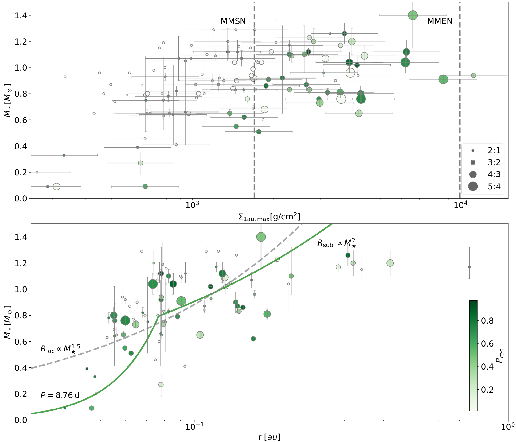
The expression $\Sigma_{\mathrm{1au,max}}\propto h_{\mathrm{1au}}^{3}$ is consistent with what Kajtazi et al. 2022 found in their simulations. In Fig. 13, we plot the $\Sigma_{\mathrm{1au,max}}$ for each planet pair that is possible in resonance, versus their host mass. The deeper the colour, the more likely it is that the pair is in resonance. The size of the symbol indicates the resonance index $j$. The figure shows that high-$j$ resonances tend to be associated with high surface densities. This result is in line with Type-I migration theory. Massive discs result in faster migration, which allows the planets to cross the relatively strong resonance. In addition, Fig. 13 shows that $\Sigma_{\mathrm{max}}$ increases with stellar mass. That is because the migration speeds in the Type I limit depend on the star-to-disc mass ratio. Higher surface density is required to migrate faster. We indicate the surface density of the Minimum mass solar nebula (Hayashi 1981, i.e., MMSN,) and the Minimum mass extra-solar nebula (Chiang & Laughlin 2013, i.e., MMEN,) in Fig. 13. The upper limits of nearly all disc surface densities are below that of the MMEN, while the inferred disc surface densities are centred around the MMSN value.

We conclude this discussion with two final points. First, the value for $\Sigma_{\mathrm{max}}$ we obtained refers to the time when the planets were locked into resonance, not the upper limit over the entire disc lifetime. Second, planets in higher $j$ resonances tend to provide higher upper limits on the disc surface density. However, they might alternatively have formed in close proximity to each other, avoiding crossing of lower-$j$ resonances. In that case, the true value of $\Sigma_{\mathrm{1au}}$ is likely to be less than $\Sigma_{\mathrm{1au,max}}$.

Planets can migrate in the disc, but their migration is believed to be halted somewhere as otherwise all planets would be consumed by the host star. However, the location and mechanism of the migration barrier are under debate. There are two main explanations for the barriers: dust sublimation (Kama et al. 2009; Flock et al. 2019) and the stellar magnetosphere (Königl et al. 2011; Hartmann et al. 2016).

If we assume a mass-luminosity relation for main sequence stars (Duric 2004), the dust sublimation radius becomes:

$$r_{\mathrm{subl}}=r_{\mathrm{sub,0}}\left(\frac{M_{\star}}{M_{\odot}}\right)^{2},$$

(34)

where $r_{\mathrm{sub,0}}$ is the silicate dust sublimation radius for solar mass stars:

$$r_{\mathrm{sub,0}}=0.13\left(\frac{C_{\mathrm{bw}}}{1}\right)^{1/2}\left(\frac{0.1}{\epsilon}\right)^{1/2}\left(\frac{1400\mathrm{K}}{T_{\mathrm{d}}}\right)^{2}\mathrm{au},$$

(35)

where $C_{\mathrm{bw}}$ is the back-warming factor, $\epsilon$ is dust cooling efficiency and $T_{\mathrm{d}}$ is the dust sublimation temperature (Kama et al. 2009).

The magnetospheric infall radius tends to expand and converge to the stellar corotation radius due to angular momentum locking (Long et al. 2005). The stellar corotation radius is expressed as:

$$r_{\mathrm{co}}=0.057\left(\frac{P_{\star}}{5\,\mathrm{d}}\right)^{\frac{2}{3}}\left(\frac{M_{\star}}{M_{\odot}}\right)^{\frac{1}{3}}\mathrm{au}$$

(36)

The rotation periods of T Tauri stars (Bouvier et al. 2007; Lee & Chiang 2017, e.g.) and young star associations (Roquette et al. 2021, e.g.,Upper Sco and NGC 2264) are several days (1-10 days).

The MCMC model is capable to identify (in a probabilistic sense) whether or not the planets have reached a migration barrier. We plot the location of the inner planet of those pairs -- the presumed location of the migration barrier -- in Fig. 13. The symbol size again represents the resonance index $j$ and the colour indicates how likely they are in resonance. From the plot, it can be seen that as the stellar mass increases the location of the migration barrier moves further away from the star. Motivated by the two theories about the migration barrier and aiming to figure out which radius is more consistent with observation, we fit the location of a migration barrier using the single power law expression:

$$r_{\mathrm{bar},k}=r_{0}\left(\frac{M_{\star,k}}{M_{\odot}}\right)^{l},$$

(37)

where $r_{0}$ is the location of the migration barrier for solar-mass stars. The Gaussian likelihood we construct is weighted by the resonance probability $P_{\mathrm{res},k}$:

$\displaystyle\ln\mathcal{L}=\sum_{k=1}^{N_{\mathrm{pairs}}}\ln\left[\mathcal{N}(r_{\mathrm{bar},k}-r_{k},\sigma_{r}^{2})\cdot P_{\mathrm{res},k}\right],$

(38)

where $r_{\mathrm{bar},k}$, $r_{k}$ and $\sigma_{r}$ are the model predicted migration barrier location for the $k$-th pair (Eq. (37)), and the presumed location of the migration barrier and the standard deviation of the fitted migration barrier radius, respectively. If one pair has a larger $P_{\mathrm{res},k}$, it is more likely that the planets are formed in the protoplanet disc and undergo disc migration. The MLE fits $r_{0}=0.13$, $l=1.49$ and $\sigma_{r}$ is 0.079 au. The location of the migration barrier fitted by single power law relation is, however, shallower than the corresponding index of the dust sublimation radius but steeper than that of the magnetospheric radius. It may imply that there are two planet populations whose migration barriers are carved by either dust sublimation radius or magnetospheric radius. For this reason, we also fit a broken power law:

$$r_{\mathrm{bar},k}=\displaystyle\left\{\begin{array}[]{ll}r_{1}\left(\frac{M_{\star,k}}{M_{\odot}}\right)^{1/3}&\text{if }M_{\star,k}\leq M_{\mathrm{crit}}\\ r_{2}\left(\frac{M_{\star,k}}{M_{\odot}}\right)^{2}&\text{if }M_{\star,k}>M_{\mathrm{crit}},\end{array}\right.$$

(39)

where $M_{\mathrm{crit}}=\left(r_{1}/r_{2}\right)^{3/5}M_{\odot}$ is the transition mass between the two different power laws. Similar to the single power law, we use MLE to fit the two parameters $r_{1}=0.08\,\mathrm{au}$ and $r_{2}=0.12\,\mathrm{au}$ and the transition mass $M_{\mathrm{crit}}$ is $0.79M_{\odot}$ (see Fig. 13). The low mass fit corresponds to a corotation period of $P_{\star}=8.76$ days, which is consistent with the observed rotation period for young stars (Bouvier et al. 2007; Lee & Chiang 2017; Roquette et al. 2021). The value of $r_{2}$ agrees with Eq. (35). Around these high-mass stars, planets are trapped at the dust sublimation location as it exceeds $r_{\mathrm{co}}$. However, the uncertainty $\sigma_{r}=0.078$ au is only slightly smaller than the value given by the single power law, suggesting that the broken power law model is only marginally better. A larger sample will make for a more reliable analysis.

References

- Agol et al. (2005) Agol E., Steffen J., Sari R., Clarkson W., 2005, MNRAS, 359, 567
- Andrews et al. (2012) Andrews S. M., et al., 2012, ApJ, 744, 162
- Ataiee & Kley (2021) Ataiee S., Kley W., 2021, arXiv e-prints, p. arXiv:2102.08612
- Bae et al. (2019) Bae J., et al., 2019, ApJ, 884, L41
- Baruteau et al. (2014) Baruteau C., et al., 2014, in Beuther H., Klessen R. S., Dullemond C. P., Henning T., eds, Protostars and Planets VI. p. 667 (arXiv:1312.4293), doi:10.2458/azu_uapress_9780816531240-ch029
- Batygin (2015) Batygin K., 2015, MNRAS, 451, 2589
- Batygin & Morbidelli (2013) Batygin K., Morbidelli A., 2013, AJ, 145, 1
- Batygin & Petit (2023) Batygin K., Petit A. C., 2023, arXiv e-prints, p. arXiv:2303.02766
- Benisty et al. (2021) Benisty M., et al., 2021, ApJ, 916, L2
- Benítez-Llambay et al. (2015) Benítez-Llambay P., Masset F., Koenigsberger G., Szulágyi J., 2015, Nature, 520, 63
- Bitsch et al. (2013) Bitsch B., Crida A., Morbidelli A., Kley W., Dobbs-Dixon I., 2013, A&A, 549, A124
- Bitsch et al. (2014) Bitsch B., Morbidelli A., Lega E., Kretke K., Crida A., 2014, A&A, 570, A75
- Bouvier et al. (2007) Bouvier J., et al., 2007, A&A, 463, 1017
- Cai et al. (2019) Cai M. X., Portegies Zwart S., Kouwenhoven M. B. N., Spurzem R., 2019, MNRAS, 489, 4311
- Caswell et al. (2021) Caswell T. A., et al., 2021, matplotlib/matplotlib: REL: v3.4.2, doi:10.5281/zenodo.592536
- Charalambous et al. (2018) Charalambous C., Martí J. G., Beaugé C., Ramos X. S., 2018, MNRAS, 477, 1414
- Charalambous et al. (2022) Charalambous C., Teyssandier J., Libert A. S., 2022, MNRAS, 514, 3844
- Chatterjee & Ford (2015) Chatterjee S., Ford E. B., 2015, ApJ, 803, 33
- Chatterjee & Tan (2014) Chatterjee S., Tan J. C., 2014, ApJ, 780, 53
- Chiang & Goldreich (1997) Chiang E. I., Goldreich P., 1997, ApJ, 490, 368
- Chiang & Laughlin (2013) Chiang E., Laughlin G., 2013, MNRAS, 431, 3444
- Choksi & Chiang (2020) Choksi N., Chiang E., 2020, MNRAS, 495, 4192
- Choksi & Chiang (2022) Choksi N., Chiang E., 2022, arXiv e-prints, p. arXiv:2211.15701
- Chrenko et al. (2022) Chrenko O., Chametla R. O., Nesvorný D., Flock M., 2022, arXiv e-prints, p. arXiv:2208.10257
- Cresswell & Nelson (2006) Cresswell P., Nelson R. P., 2006, A&A, 450, 833
- Cresswell & Nelson (2008) Cresswell P., Nelson R. P., 2008, A&A, 482, 677
- D’Angelo & Lubow (2010) D’Angelo G., Lubow S. H., 2010, ApJ, 724, 730
- Dai et al. (2022) Dai F., et al., 2022, arXiv e-prints, p. arXiv:2210.09283
- Dawson et al. (2015) Dawson R. I., Chiang E., Lee E. J., 2015, MNRAS, 453, 1471
- Delisle & Laskar (2014) Delisle J. B., Laskar J., 2014, A&A, 570, L7
- Duric (2004) Duric N., 2004, Advanced astrophysics
- Fabrycky et al. (2014) Fabrycky D. C., et al., 2014, ApJ, 790, 146
- Fitzmaurice et al. (2022) Fitzmaurice E., Martin D. V., Fabrycky D. C., 2022, MNRAS, 512, 5023
- Flock et al. (2019) Flock M., Turner N. J., Mulders G. D., Hasegawa Y., Nelson R. P., Bitsch B., 2019, A&A, 630, A147
- Foreman-Mackey (2016) Foreman-Mackey D., 2016, The Journal of Open Source Software, 1, 24
- Foreman-Mackey et al. (2013) Foreman-Mackey D., Hogg D. W., Lang D., Goodman J., 2013, PASP, 125, 306
- Fortney et al. (2007) Fortney J. J., Marley M. S., Barnes J. W., 2007, ApJ, 659, 1661
- Fulton & Petigura (2018) Fulton B. J., Petigura E. A., 2018, AJ, 156, 264
- Fulton et al. (2017) Fulton B. J., et al., 2017, AJ, 154, 109
- Garrido-Deutelmoser et al. (2023) Garrido-Deutelmoser J., Petrovich C., Charalambous C., Guzmán V. V., Zhang K., 2023, arXiv e-prints, p. arXiv:2301.13260
- Ge et al. (2022) Ge J., et al., 2022, arXiv e-prints, p. arXiv:2206.06693
- Ghosh & Chatterjee (2022) Ghosh T., Chatterjee S., 2022, arXiv e-prints, p. arXiv:2209.05138
- Gillon et al. (2017) Gillon M., et al., 2017, Nature, 542, 456
- Ginzburg et al. (2018) Ginzburg S., Schlichting H. E., Sari R., 2018, MNRAS, 476, 759
- Goldberg & Batygin (2022) Goldberg M., Batygin K., 2022, arXiv e-prints, p. arXiv:2211.16725
- Goldreich & Schlichting (2014) Goldreich P., Schlichting H. E., 2014, AJ, 147, 32
- Goldreich & Tremaine (1979) Goldreich P., Tremaine S., 1979, ApJ, 233, 857
- Goldreich & Tremaine (1980) Goldreich P., Tremaine S., 1980, ApJ, 241, 425
- Guilera et al. (2019) Guilera O. M., Cuello N., Montesinos M., Miller Bertolami M. M., Ronco M. P., Cuadra J., Masset F. S., 2019, MNRAS, 486, 5690
- Guilera et al. (2021) Guilera O. M., Miller Bertolami M. M., Masset F., Cuadra J., Venturini J., Ronco M. P., 2021, MNRAS, 507, 3638
- Hartmann et al. (2016) Hartmann L., Herczeg G., Calvet N., 2016, ARA&A, 54, 135
- Hayashi (1981) Hayashi C., 1981, Progress of Theoretical Physics Supplement, 70, 35
- Hayya et al. (1975) Hayya J., Armstrong D., Gressis N., 1975, Management Science, 21, 1338
- Hinkley (1969) Hinkley D. V., 1969, Biometrika, 56, 635
- Huang & Ormel (2022) Huang S., Ormel C. W., 2022, MNRAS, 511, 3814
- Hunter (2007) Hunter J. D., 2007, Computing in Science and Engineering, 9, 90
- Ida & Lin (2004) Ida S., Lin D. N. C., 2004, ApJ, 604, 388
- Ida et al. (2020) Ida S., Muto T., Matsumura S., Brasser R., 2020, MNRAS, 494, 5666
- Isella et al. (2018) Isella A., et al., 2018, ApJ, 869, L49
- Izidoro et al. (2017) Izidoro A., Ogihara M., Raymond S. N., Morbidelli A., Pierens A., Bitsch B., Cossou C., Hersant F., 2017, MNRAS, 470, 1750
- Izidoro et al. (2021) Izidoro A., Bitsch B., Raymond S. N., Johansen A., Morbidelli A., Lambrechts M., Jacobson S. A., 2021, A&A, 650, A152
- Izidoro et al. (2022) Izidoro A., Schlichting H. E., Isella A., Dasgupta R., Zimmermann C., Bitsch B., 2022, ApJ, 939, L19
- Jiang & Ormel (2023) Jiang H., Ormel C. W., 2023, MNRAS, 518, 3877
- Kajtazi et al. (2022) Kajtazi K., Petit A. C., Johansen A., 2022, arXiv e-prints, p. arXiv:2211.06181
- Kama et al. (2009) Kama M., Min M., Dominik C., 2009, A&A, 506, 1199
- Kanagawa et al. (2018) Kanagawa K. D., Tanaka H., Szuszkiewicz E., 2018, ApJ, 861, 140
- Königl et al. (2011) Königl A., Romanova M. M., Lovelace R. V. E., 2011, MNRAS, 416, 757
- Laune et al. (2022) Laune J. T., Rodet L., Lai D., 2022, MNRAS, 517, 4472
- Lee & Chiang (2017) Lee E. J., Chiang E., 2017, ApJ, 842, 40
- Leemker et al. (2022) Leemker M., et al., 2022, A&A, 663, A23
- Lin & Papaloizou (1979) Lin D. N. C., Papaloizou J., 1979, MNRAS, 186, 799
- Lithwick & Wu (2012) Lithwick Y., Wu Y., 2012, ApJ, 756, L11
- Liu et al. (2017) Liu B., Ormel C. W., Lin D. N. C., 2017, A&A, 601, A15
- Liu et al. (2019) Liu B., Lambrechts M., Johansen A., Liu F., 2019, A&A, 632, A7
- Long et al. (2005) Long M., Romanova M. M., Lovelace R. V. E., 2005, ApJ, 634, 1214
- Luger et al. (2017) Luger R., et al., 2017, Nature Astronomy, 1, 0129
- Luque & Pallé (2022) Luque R., Pallé E., 2022, Science, 377, 1211
- Masset (2017) Masset F. S., 2017, MNRAS, 472, 4204
- Masset et al. (2006) Masset F. S., Morbidelli A., Crida A., Ferreira J., 2006, ApJ, 642, 478
- Mayor & Queloz (1995) Mayor M., Queloz D., 1995, Nature, 378, 355
- Mordasini et al. (2015) Mordasini C., Mollière P., Dittkrist K. M., Jin S., Alibert Y., 2015, International Journal of Astrobiology, 14, 201
- Murray & Dermott (1999) Murray C. D., Dermott S. F., 1999, Solar system dynamics
- Ogihara & Kobayashi (2013) Ogihara M., Kobayashi H., 2013, ApJ, 775, 34
- Ogihara et al. (2018) Ogihara M., Kokubo E., Suzuki T. K., Morbidelli A., 2018, A&A, 615, A63
- Owen & Wu (2013) Owen J. E., Wu Y., 2013, ApJ, 775, 105
- Owen & Wu (2017) Owen J. E., Wu Y., 2017, ApJ, 847, 29
- Paardekooper et al. (2010) Paardekooper S. J., Baruteau C., Crida A., Kley W., 2010, MNRAS, 401, 1950
- Paardekooper et al. (2011) Paardekooper S. J., Baruteau C., Kley W., 2011, MNRAS, 410, 293
- Papaloizou & Larwood (2000) Papaloizou J. C. B., Larwood J. D., 2000, MNRAS, 315, 823
- Papaloizou & Szuszkiewicz (2005) Papaloizou J. C. B., Szuszkiewicz E., 2005, MNRAS, 363, 153
- Papaloizou et al. (2018) Papaloizou J. C. B., Szuszkiewicz E., Terquem C., 2018, MNRAS, 476, 5032
- Petigura et al. (2018) Petigura E. A., et al., 2018, AJ, 156, 89
- Piaulet et al. (2022) Piaulet C., et al., 2022, Nature Astronomy,
- Pichierri et al. (2022) Pichierri G., Bitsch B., Lega E., 2022, arXiv e-prints, p. arXiv:2212.03608
- Ramos et al. (2017) Ramos X. S., Charalambous C., Benítez-Llambay P., Beaugé C., 2017, A&A, 602, A101
- Rauer et al. (2014) Rauer H., et al., 2014, Experimental Astronomy, 38, 249
- Raymond et al. (2008) Raymond S. N., Barnes R., Mandell A. M., 2008, MNRAS, 384, 663
- Rein (2012) Rein H., 2012, MNRAS, 427, L21
- Rein & Liu (2012) Rein H., Liu S. F., 2012, A&A, 537, A128
- Rein & Papaloizou (2009) Rein H., Papaloizou J. C. B., 2009, A&A, 497, 595
- Ribas et al. (2014) Ribas Á., Merín B., Bouy H., Maud L. T., 2014, A&A, 561, A54
- Romanova et al. (2019) Romanova M. M., Lii P. S., Koldoba A. V., Ustyugova G. V., Blinova A. A., Lovelace R. V. E., Kaltenegger L., 2019, MNRAS, 485, 2666
- Roquette et al. (2021) Roquette J., Matt S. P., Winter A. J., Amard L., Stasevic S., 2021, MNRAS, 508, 3710
- Ruden & Lin (1986) Ruden S. P., Lin D. N. C., 1986, ApJ, 308, 883
- Sánchez et al. (2020) Sánchez M. B., de Elía G. C., Downes J. J., 2020, A&A, 637, A78
- Seager et al. (2007) Seager S., Kuchner M., Hier-Majumder C. A., Militzer B., 2007, ApJ, 669, 1279
- Snellgrove et al. (2001) Snellgrove M. D., Papaloizou J. C. B., Nelson R. P., 2001, A&A, 374, 1092
- Steffen & Hwang (2015) Steffen J. H., Hwang J. A., 2015, MNRAS, 448, 1956
- Stock et al. (2020) Stock K., Cai M. X., Spurzem R., Kouwenhoven M. B. N., Portegies Zwart S., 2020, MNRAS, 497, 1807
- Tamayo et al. (2020) Tamayo D., Rein H., Shi P., Hernand ez D. M., 2020, MNRAS, 491, 2885
- Tanaka & Ward (2004) Tanaka H., Ward W. R., 2004, ApJ, 602, 388
- Tanaka et al. (2002) Tanaka H., Takeuchi T., Ward W. R., 2002, ApJ, 565, 1257
- Terquem & Papaloizou (2007) Terquem C., Papaloizou J. C. B., 2007, ApJ, 654, 1110
- Terquem & Papaloizou (2019) Terquem C., Papaloizou J. C. B., 2019, MNRAS, 482, 530
- Teske et al. (2021) Teske J., et al., 2021, ApJS, 256, 33
- Teyssandier & Libert (2020) Teyssandier J., Libert A.-S., 2020, A&A, 643, A11
- Teyssandier & Terquem (2014) Teyssandier J., Terquem C., 2014, MNRAS, 443, 568
- Wang & Ji (2014) Wang S., Ji J., 2014, ApJ, 795, 85
- Ward (1986) Ward W. R., 1986, Icarus, 67, 164
- Ward (1991) Ward W. R., 1991, in Lunar and Planetary Science Conference. p. 1463
- Ward (1992) Ward W. R., 1992, in Lunar and Planetary Science Conference. p. 1491
- Ward (1997) Ward W. R., 1997, Icarus, 126, 261
- Weidenschilling (1977) Weidenschilling S. J., 1977, MNRAS, 180, 57
- Winter et al. (2019) Winter A. J., Clarke C. J., Rosotti G. P., Hacar A., Alexander R., 2019, MNRAS, 490, 5478
- Wolfgang et al. (2016) Wolfgang A., Rogers L. A., Ford E. B., 2016, ApJ, 825, 19
- Xie (2014) Xie J.-W., 2014, ApJ, 786, 153
- Ye (2022) Ye Y., 2022, Nature, 604, 415
- Zhu & Dong (2021) Zhu W., Dong S., 2021, ARA&A, 59, 291
Appendix A Results of the General disc model
The full MCMC fitting corner plot of the General model is shown in Fig. 14. The fitted values for all four parameters are , , . However, these values do not necessarily refer to the real physical disc parameters, due to the degeneracy among them. Therefore, we generate mock planet period ratio data (with the same size as our sample used here) and examine this MCMC model without specifying the disc structure in Sect. B.1. Those tests indeed suggest that and are not able to be retrieved.
Fig. 14 reveals the degeneracy: negatively correlates with , correlates positively with and positively with . We found that such correlations are well represented by: