Exemplars and Counterexemplars Explanations for Image Classifiers, Targeting Skin Lesion Labeling

The image $x{\in}\mathbb{R}^{n}$ to be explained is passed as input to the AAE where the $\mathit{encoder}$ returns the latent representation $z\in\mathbb{R}^{k}$ using $k$ latent features with ${k\ll n}$.

abele generates a set $H$ of $N$ instances in the latent feature space, with characteristics close to those of $z$. Since the goal is to learn a predictor on $H$ able to simulate the local behavior of $b$, the neighborhood includes instances with both decisions, i.e., $H=H_{=}\cup H_{\neq}$ where instances $h\in H_{=}$ are such that $b(\widetilde{h})=b(x)$, and $h\in H_{\neq}$ are such that $b(\widetilde{h})\neq b(x)$. We name $\widetilde{h}\in\mathbb{R}^{n}$ the decoded version of an instance $h\in\mathbb{R}^{k}$ in the latent feature space. The neighborhood generation of $H$ ($\mathit{neighgen}$ module in Fig. 2) may be accomplished using different strategies ranging from pure random strategy using a given distribution to a genetic approach maximizing a fitness function [18]. In our experiments we adopt the last strategy. After the generation process, for any instance $h\in H$, abele exploits the $\mathit{disde}$ module (Fig. 1-right) for both checking the validity of $h$ by querying the $\mathit{discriminator}$ and decoding it into $\widetilde{h}$. Then, it queries the black box $b$ with $\widetilde{h}$ to get the class $y$, i.e., $b(\widetilde{h})=y$.

Given the local neighborhood $H$, abele builds a decision tree classifier $c$ trained on $H$ labeled with $b(\widetilde{H})$. The surrogate tree is intended to locally mimic the behavior of $b$ in the neighborhood $H$. It extracts the decision rule $r$ and counter-factual rules $\Phi$ enabling the generation of exemplars and counter-exemplars. Fig. 2 shows the process that, starting from the image to be explained, leads to the decision tree learning, and to the extraction of the decision and counter-factual rules. We name this module llore, as a variant of lore [18].

Often, e.g. in medical or managerial decision making, people explain their decisions by pointing to exemplars with the same (or different) decision outcome. We follow this approach and we model the explanation of an image $x$ returned by abele as a triple ${e=\langle\widetilde{H}_{e},\widetilde{H}_{c},s\rangle}$ composed by exemplars $\widetilde{H}_{e}$, counter-exemplars $\widetilde{H}_{c}$ and a saliency map $s$. Exemplars and counter-exemplars are images representing instances similar to $x$, leading to an outcome equal to or different from $b(x)$. Exemplars and counter-exemplars are generated by abele exploiting the $\mathit{eg}$ module (Fig. 3-left). It first generates a set of latent instances $H$ satisfying the decision rule $r$ (or a set of counter-factual rules $\Phi$), as shown in Fig. 2. Then, it validates and decodes them into exemplars $\widetilde{H}_{e}$ (or counter-exemplars $\widetilde{H}_{c}$) using the $\mathit{disde}$ module. The saliency map $s$ highlights areas of $x$ that contribute to its outcome and areas that push it into another class. The map is obtained by the saliency extractor $\mathit{se}$ module (Fig. 3-right) that first computes the pixel-to-pixel-difference between $x$ and each exemplar in the set $\widetilde{H}_{e}$, and then, it assigns to each pixel of the saliency map $s$ the median value of all differences calculated for that pixel. Thus, formally for each pixel $i$ of the saliency map $s$ we have: $s[i]=\mathit{median}_{\forall\widetilde{h}_{e}\in\widetilde{H}_{e}}(x[i]-\widetilde{h}_{e}[i]).$

The dataset is composed of a training set of 25,331 JPEG images of skin lesions and their category (labels); a test set of 8,238 unlabelled JPEG images of skin lesions. In our experiments we relied on the training set for which ground truth is directly available. In particular, from the training set, we used $80\%$ for training and $20\%$ for validation. For the evaluation, we use the same evaluation protocols as the submission system.

Since the images have different resolutions. We preprocess them as follows:

• •

  For the training process, the images are randomly rescaled, rotated and cropped to generate the input to the network. Note that such preprocessing does not deform the lesions in the image. Resolution of the preprocessed images is 224×224.

• •

  For the validation and test process, each image is firstly rescaled to 256×256 according to the shorter edge, then cropped at the center into a 224×224 image.

Since the UNK category is a reject option and is not available in the training we focused on the 8 other categories.

For the classification, we used a classical ResNet, pretrained on Imagenet, i.e., a black box classifier. In particular, we replaced the last classification layer by the new one adapted to the number of classes in the diagnosis. We trained this layer and fine tuned the rest of the network on ISIC dataset. The $50$-layer ResNet architecture is the following: The network is composed of 18 modules sequentially combined together, including one conv1 module (7×7, 64 filters, stride 2), three conv2 modules (1×1, 64 filters, stride 1; 3×3, 64 filters, stride 1; 1×1, 256 filters, stride 1), four conv3 (1×1, 128 filters, stride 2; 3×3, 128 filters, stride 1; 1×1, 512 filters, stride 1), six conv4 (1×1, 256 filters, stride 2; 3×3, 256 filters, stride 1; 1×1, 1024 filters, stride 1), three conv5 (1×1, 512 filters, stride 2; 3×3, 512 filters, stride 1; 1×1, 2048 filters, stride 1) and one last fully connected module fc (average pooling, 9-output fully connected layer, sigmoid activation). The first module conv1 is composed of one single convolution layer. For conv2 to conv5, each module is a residual block including three convolutional layers in the residual branch. The output of such block is the sum of the input and the output of the convolutional layers. The module fc is the newly trained prediction layer. The spatial size is reduced only at the first layer of the modules conv3, conv4 and conv5. We adopt a binary cross entropy loss for each class, so that the problem is considered as 8 individual one-vs-rest binary classification problems.

The official evaluation criterion for the challenge is the Normalized (or balanced) multi-class accuracy. It is defined as the average of recall obtained in each class. The best value is 1 and the worst is 0. This metric makes all the classes equally important. In terms of balanced multi-class accuracy (mean value of categorical recalls), the trained model achieved 0.838 on the validation set. We report also the performance on the official test set. The score is 0.488, which is potentially impacted by the presence of out-of-distribution samples (UNK) since the model was not tuned for rejection.

Generative Adversarial models are generally not easy to train as they are usually affected by a number of common failures. These problems vary from a diversified spectrum of failures in convergence to the famous Mode Collapse [19], the tendency by the generator network to produce a small variety of output types. Such problems mainly arise from the competing scheme generator and discriminator are trained on: they are trained simultaneously in a zero-sum game, thus the goal is to find an equilibrium between the two competing objectives. Since every time the parameters of one of the models are updated the nature of the optimization problem is changed, this has the effect of creating a dynamic system that easily fails to converge.

Furthermore, even the concept of convergence is not as clear as in other context. As the generator improves during the training, the discriminator performance gets worse because it cannot easily tell the difference between real and fake outputs. At the limit where the generator succeeds perfectly, the discriminator flips a coin to make its prediction. Hence, the discriminator feedback gets less meaningful over time. If the model continues training past the point when the discriminator is giving random feedback, then the generator starts to train on low quality feedback, and its own performance may collapse. For a Generative Adversarial model, convergence is often an unstable transitory region rather than a stable state.
In addition to the previous problems, we often face the further complication to deal with real world datasets that are far from ideal: fragmentation, imbalance, lack of uniform digitization, shortage of data are primary challenges of big data analytics for healthcare. All of them impede efficiency and accuracy of machine learning model trained with these data, especially in the case of inherently fragile generative models.

Training an AAE in a standard fashion to reproduce samples from ISIC dataset without taking special care of all issues mentioned above resulted in extremely poor performance, mostly due to a persistent collapse mode. In order to overcome such generative failure and dataset limitations, we implemented a collection of cutting edge techniques that altogether is capable of addressing all the issues we mentioned and successfully training an AAE with adequate performance.

One usually wants a generative model to produce a large variety of outputs, for example, a different image for every input of our skin lesion generator. However, since the generator is always trying to produce the one output that seems most plausible to the discriminator, it may happen that the generator learns to produce just a single output over and over again, or a small set of outputs. In such case, the discriminator best strategy is to learn to always reject that output. But if the current discriminator gets stuck in a poor local minimum it is not going to find the best strategy, hence it would be too easy for the generator to find the most credible output for the current discriminator.

As a consequence, at each iteration of generator an over-optimization for the current discriminator takes place, and the discriminator never learns to escape out of the trap. Thus, each generation of generator rotates through a small set of output types, possibly a single one. In adversarial generative models, this form of failure is called mode collapse.

In recent years many techniques have been proposed to overcome this ubiquitous form of failure. Ad hoc tricks like Mini Batch Discrimination [20] or Wasserstein Loss [21] have been proved empirically to alleviates mode collapse, while Unrolled GANs [22] or Conditional AAE [23] intervene directly on the internal structure of the training scheme to discouraging over-optimization by the current generator.

The reasons behind mode collapse and other forms of failure remain still unclear and not fully proven. In the health domain, such singularities around the train process appear to be even more frequent. Possible reasons can be the lack of a substantial number of training data, the necessity to deal with high resolution images, fragmented and highly unbalanced datasets (malignant cancers are usually a small proportion of the entire batch). Furthermore, the need of a substantial number of latent features makes the parameter space extremely irregular, non-convex and in need of powerful regularization. In order to overcome failure modes and train an AAE successfully, we used the following collection of techniques.

Progressive Growing GANs [24] have been introduced as an extension to the GANs training process. It helps to achieve a more stable training of generative models for high resolution images. The main idea is to start with a very low resolution image and step by step adding block of layers that simultaneously increase the output size of the generator model and the input size of the discriminator model until the desired size is achieved.

In a general GAN scheme, the discriminator is linked to the generator model output. However, in an AAE the discriminator takes as input the encoded latent space instead of the full reconstructed image. In order to achieve all benefits of a progressive growing model, we need a novel structure to take care of this different dynamics. We then propose a Progressive Growing Adversarial Autoencoder (PGAAE): starting with a single block of convolutional layers for each of the two generating networks (encoder and decoder) we are able to reconstruct low resolution images (7x7 pixels), then step by step we increase the number of blocks until the network is powerful enough to manage images of the desired size (224x224 pixels). The latent space dimension is kept fixed, consequently the discriminator takes as input tensors always the same size. Although one could fix also the discriminator network, we found helpful to progressively increasing also the width of this network so that the discriminator can deal each step with a more structured information. On the contrary, we observe that increasing the depth of the discriminator increases the instability of the training, causing a wide variety of failures ranging from poor performance to catastrophic forgetting [19].

The main idea behind such construction relies on the instability caused to the training process by heavy structured high dimensional data. Generating high-resolution images is challenging for generative models, as the generator must learn how to output both high dimensional structure and fine details at the same time. The high resolution makes any discrepancy in the fine detail of generated images easy to mark for the discriminator, and the training process degenerates. Large images also require significantly more memory, consequently, the batch size used to update model weights each iteration is reduced to ensure that the large images fit into memory. This introduces further instability into the process.

The incremental addition of the layers allows the models to first learn large scale structure and progressively shift the attention to finer detail. At each step, all previous layers remain trainable throughout the training process. From a different point of view, one can think of each block of layers as the initialization of the same common network structure of the subsequent step of the progressive scheme. Such progressive initialization is by all means a powerful form of regularization carried out through both the encoder and decoder networks. A heavy quantity of regularization is indeed needed to smooth the parameter space and, in turn, reducing failure modes like mode collapse.

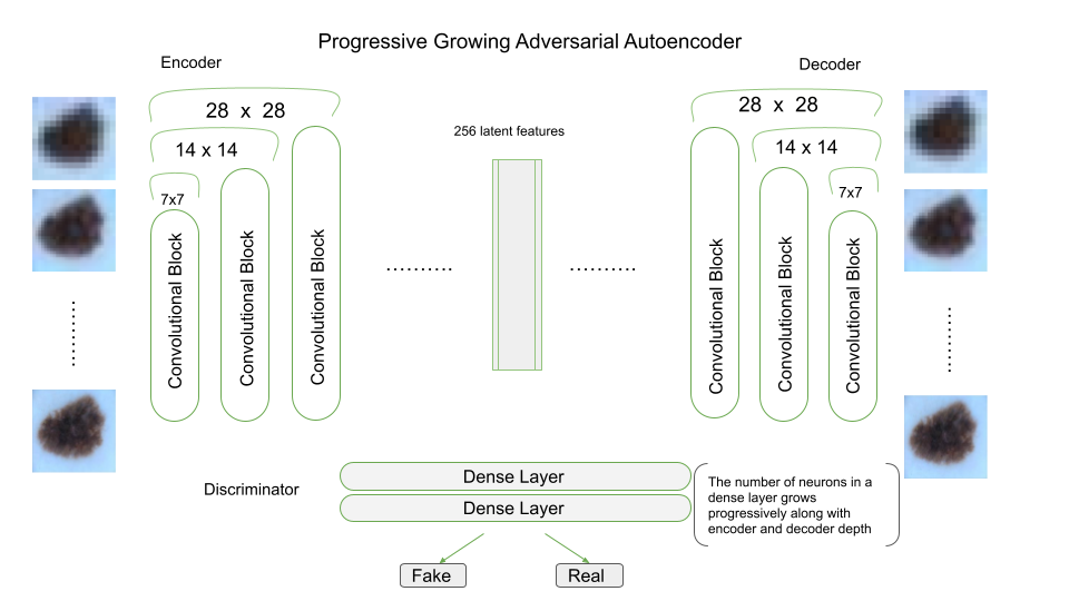
The PGAAE network paradigma is reported in Figure 5. First, we start by training a shallow AAE with just one convolutional block for both the encoder and decoder network. Such first AAE is trained to reconstruct skin lesion images resized to 7x7 pixels. Once the network is fully trained and optimized, it sends its weights to a second AAE with a deeper structure of two convolutional blocks for both the encoder and decoder network. This second AAE is trained with the same dataset resized to 14x14 pixels. At each step, weights are shared just over the common underlying structure and then kept trainable for future training steps, i.e. each AAE is initialized with the previous AAE weights and trained with images doubled in size.

After the sixth step, we have a fully trained AAE able to reproduce skin lesion images of size 224x224 pixels. In order to enhance the discriminator ability to discriminate between more and more complex images, at each step the discriminator grows in width: it consists of two dense layers with a progressive growing number of neurons (from 500 to 3000 with a step increase of 500 neurons after each phase) and a Leaky ReLu activation with parameter $0.2$. All discriminators end with a single neuron dense layer with a sigmoid activation.

Each convolutional block includes two identical sets of three layers: a conv2d layer with stride 3, filters ranging from 16 to 128, followed by a batch normalization with parameter 0.95 and a ReLu activation. Depending on whether we consider the encoder or the decoder network, a max pooling or an up sampling layer is attached at the end of each block.

Another major issue affecting the training of generative models is the tendency of learning the identity function: if the autoencoder has more nodes in the hidden layer than inputs, then it can just learn the data and the output simply equals the input. Hence, it does not perform any useful representation learning or dimensionality reduction.

Denoising autoencoders [25] are a stochastic version of basic autoencoders. A Denoising autoencoder attempts to address the identity function issue by randomly corrupting input images that the autoencoder must then reconstruct. By making the training process and the reconstruction phase more challenging, it is proved that denoising autoencoders mitigate the identity function issue and learn more robust representations.

Another way to gain more generalization, reduce the vanishing gradient problem and improve convergence is to add noise also to the discriminator inputs [26]. Denoising autoencoder, adversarial generative training ad noise injection have been used separately to improve autoencoder performance. We augment the adversarial model with both a denoising feature applied to the generator and a noise injection in to the discriminator. The denoising feature was particularly helpful in achieving good reconstruction performance for latent space with 256 latent features. We opted for a Gaussian noise with standard deviation $\sigma=0.1$ (we tried different value ranging from $0.05$ to $0.9$: it seems there is no significant difference in reconstruction accuracy in the range $\sigma\in[0.1,0.3]$; accuracy starts to deteriorate quickly after $\sigma=0.3$). Despite we are not interested in low dimensional latent space (reconstructed images would be too blurry and not enough variegate), we found no significant advantage in injecting noise in such cases.

Mini Batch Discrimination [20] was originally introduced as a technique to mitigate collapse of the generator network. It is a discriminative technique for generative adversarial networks between whole minibatches of samples rather than between individual samples.

The idea is for the discriminator to consider an entire batch of data, instead of looking to a single input data. The mode collapse is then much easier to spot, since the discriminator understands that whenever all the samples in a batch are very close to each other, the data has to be rejected. This forces the generator to produce many good outputs in each data batch. An $L_{1}$ penalization norm is concatenated with the original input and fed to the discriminator last but one layer. Such penalization quantifies the closeness between data in the same minibatch, causing the discriminator to reject batches that are internally too similar. This discriminative technique along with the progressive growing network structure, helped to avoid the mode collapse for batches of small and middle size (16-64) at the cost of a small increase of discriminator parameters. Indeed, training AAE with small batches size increases the chances of falling in to a mode collapse. However, small batch sizes are forced by hardware limitation due to high resolution images and high dimensional latent space.

Following [20], a minibatch discrimination layer needs two hyperparameters to be fine tuned, namely $B$ and $C$ in the original paper, i.e. the number of discrimination kernels to use and the dimensionality of the space where closeness of samples is calculated. Hypothetically, the larger $B$ and $C$ are, the better results are obtained at the price of a lower computation speed. A good compromise between accuracy and speed was the choice $B=16$ and $C=5$.

After a thorough fine tuning of all three networks structures (encoder, decoder and discriminator) our PGAAE with 256 latent features achieves a reconstruction error measure through RMSE that ranges from $0.08$ to $0.24$ depending on whether we consider the most common or the most rare skin lesion class. Data augmentation was necessary to overcome scarcity and imbalance of the dataset. Mode collapse is greatly reduced, and we are able to generate variegate and good quality skin lesion images. ABELE explainer is now able to generate meaningful explanations.

References

- [1] D. Pedreschi, F. Giannotti, R. Guidotti, A. Monreale, S. Ruggieri, and F. Turini, “Meaningful explanations of black box AI decision systems,” in AAAI. AAAI Press, 2019, pp. 9780–9784.
- [2] I. Iqbal, M. Younus, K. Walayat, M. U. Kakar, and J. Ma, “Automated multi-class classification of skin lesions through deep convolutional neural network with dermoscopic images,” Comput. Medical Imaging Graph., vol. 88, p. 101843, 2021.
- [3] Q. Li, W. Cai, X. Wang, Y. Zhou, D. D. Feng, and M. Chen, “Medical image classification with convolutional neural network,” in ICARCV. IEEE, 2014, pp. 844–848.
- [4] M. Antonie, O. R. Zaïane, and A. Coman, “Application of data mining techniques for medical image classification,” in MDM/KDD. University of Alberta, 2001, pp. 94–101.
- [5] A. Adadi and M. Berrada, “Peeking inside the black-box: A survey on explainable artificial intelligence (XAI),” IEEE Access, vol. 6, pp. 52 138–52 160, 2018.
- [6] T. Miller, “Explanation in artificial intelligence: Insights from the social sciences,” Artif. Intell., vol. 267, pp. 1–38, 2019.
- [7] R. Guidotti, A. Monreale, S. Ruggieri, F. Turini, F. Giannotti, and D. Pedreschi, “A survey of methods for explaining black box models,” ACM Comput. Surv., vol. 51, no. 5, pp. 93:1–93:42, 2019.
- [8] C. Panigutti, A. Perotti, and D. Pedreschi, “Doctor XAI: an ontology-based approach to black-box sequential data classification explanations,” in FAT*. ACM, 2020, pp. 629–639.
- [9] M. T. Ribeiro, S. Singh, and C. Guestrin, “”why should I trust you?”: Explaining the predictions of any classifier,” in KDD. ACM, 2016, pp. 1135–1144.
- [10] S. M. Lundberg and S. Lee, “A unified approach to interpreting model predictions,” in NIPS, 2017, pp. 4765–4774.
- [11] R. Guidotti, A. Monreale, and L. Cariaggi, “Investigating neighborhood generation methods for explanations of obscure image classifiers,” in PAKDD (1), ser. Lecture Notes in Computer Science, vol. 11439. Springer, 2019, pp. 55–68.
- [12] R. Guidotti, A. Monreale, S. Matwin, and D. Pedreschi, “Black box explanation by learning image exemplars in the latent feature space,” in ECML/PKDD (1), ser. Lecture Notes in Computer Science, vol. 11906. Springer, 2019, pp. 189–205.
- [13] M. Sundararajan et al., “Axiomatic attribution for dnn,” in ICML. JMLR, 2017.
- [14] A. Shrikumar, P. Greenside, A. Shcherbina, and A. Kundaje, “Not just a black box: Learning important features through propagating activation differences,” CoRR, vol. abs/1605.01713, 2016.
- [15] S. Bach, A. Binder et al., “On pixel-wise explanations for non-linear classifier decisions by layer-wise relevance propagation,” PloS one, vol. 10, no. 7, p. e0130140, 2015.
- [16] A. Makhzani, J. Shlens, N. Jaitly, and I. J. Goodfellow, “Adversarial autoencoders,” CoRR, vol. abs/1511.05644, 2015.
- [17] I. J. Goodfellow, J. Pouget-Abadie, M. Mirza, B. Xu, D. Warde-Farley, S. Ozair, A. C. Courville, and Y. Bengio, “Generative adversarial nets,” in NIPS, 2014, pp. 2672–2680.
- [18] R. Guidotti, A. Monreale, F. Giannotti, D. Pedreschi, S. Ruggieri, and F. Turini, “Factual and counterfactual explanations for black box decision making,” IEEE Intell. Syst., vol. 34, no. 6, pp. 14–23, 2019.
- [19] H. Thanh-Tung and T. Tran, “Catastrophic forgetting and mode collapse in gans,” in IJCNN, 2020.
- [20] T. Salimans, I. Goodfellow, W. Zaremba, V. Cheung, A. Radford, X. Chen, and X. C. and, “Improved techniques for training gans,” in NIPS, 2016.
- [21] Y. Dukler, W. Li, A. Lin, and G. Montufar, “Wasserstein of wasserstein loss for learning generative models,” in Proceedings of the 36th International Conference on Machine Learning, 2019.
- [22] L. Metz, B. Poole, D. Pfau, and J. Sohl-Dickstein, “Unrolled generative adversarial networks,” in ICLR, 2017.
- [23] Z. Zhang, Y. Song, and H. Qi, “Age progression/regression by conditional adversarial autoencoder,” in IEEE Conference on Computer Vision and Pattern Recognition, 2017.
- [24] T. Karras, T. Aila, S. Laine, and J. Lehtinen, “Progressive growing of gans for improved quality, stability, and variation,” in ICLR, 2018.
- [25] P. Vincent, H. Larochelle, Y. Bengio, and P.-A. Manzagol, “Extracting and composing robust features with denoising autoencoders,” in ICML, 2008.
- [26] M. Arjovsky and L. Bottou, “Towards principled methods for training generative adversarial networks,” in ICLR, 2017.