Spectral Augmentations for Graph Contrastive Learning
Amur Ghose Yingxue Zhang Jianye Hao Mark Coates
Huawei Huawei Huawei, Tianjin University McGill
Abstract
Contrastive learning has emerged as a premier method for learning representations with or without supervision. Recent studies have shown its utility in graph representation learning for pre-training. Despite successes, the understanding of how to design effective graph augmentations that can capture structural properties common to many different types of downstream graphs remains incomplete. We propose a set of well-motivated graph transformation operations derived via graph spectral analysis to provide a bank of candidates when constructing augmentations for a graph contrastive objective, enabling contrastive learning to capture useful structural representation from pre-training graph datasets. We first present a spectral graph cropping augmentation that involves filtering nodes by applying thresholds to the eigenvalues of the leading Laplacian eigenvectors. Our second novel augmentation reorders the graph frequency components in a structural Laplacian-derived position graph embedding. Further, we introduce a method that leads to improved views of local subgraphs by performing alignment via global random walk embeddings. Our experimental results indicate consistent improvements in out-of-domain graph data transfer compared to state-of-the-art graph contrastive learning methods, shedding light on how to design a graph learner that is able to learn structural properties common to diverse graph types.
1 Introduction
Representation learning is of perennial importance, with contrastive learning being a recent prominent technique. Taking images as an example, under this framework, a set of transformations is applied to image samples, without changing the represented object or its label. Candidate transformations include cropping, resizing, Gaussian blur, and color distortion. These transformations are termed augmentations (Chen et al. 2020b; Grill et al. 2020). A pair of augmentations from the same sample are termed positive pairs. During training, their representations are pulled together (Khosla et al. 2020). In parallel, the representations from negative pairs, consisting of augmentations from different samples, are pushed apart. The contrastive objective encourages representations that are invariant to distortions but capture useful features. This constructs general representations, even without labels, that are usable downstream.
Recently, self-supervision has been employed to support the training process for graph neural networks (GNNs). Several approaches (e.g., Deep Graph Infomax (DGI) (Velickovic et al. 2019), InfoGCL (Xu et al. 2021)) rely on mutual information maximization or information bottlenecking between pairs of positive views. Other GNN pre-training strategies construct objectives or views that rely heavily on domain-specific features (Hu et al. 2020b; Hu et al. 2020c). This inhibits their ability to generalize to other application domains. Some recent graph contrastive learning strategies such as GCC (Qiu et al. 2020) and GraphCL (You et al. 2020) can more readily transfer knowledge to out-of-domain graph domains, because they derive embeddings based solely on local graph structure, avoiding possibly unshared attributes entirely. However, these approaches employ heuristic augmentations such as random walk with restart and edge-drop, which are not designed to preserve graph properties and might lead to unexpected changes in structural semantics (Lee et al. 2022). There is a lack of diverse and effective graph transformation operations to generate augmentations. We aim to fill this gap with a set of well-motivated graph transformation operations derived via graph spectral analysis to provide a bank of candidates when constructing augmentations for a graph contrastive objective. This allows the graph encoder to learn structural properties that are common for graph data spanning multiple graphs and domains.
| Approaches | Goal is pre-training or transfer | No requirement for features | Domain transfer | Shareable graph encoder |
| Category 1 (DGI, InfoGraph, MVGRL, DGCL, InfoGCL, AFGRL) | ✗ | ✗ | ✗ | ✗ |
| Category 2 (GPT-GNN, Strategies for pre-training GNNs) | ✔ | ✗ | ✗ | ✔ |
| Category 3 (Deepwalk, LINE, node2vec) | ✗ | ✔ | ✔ | ✗ |
| Category 4 (struc2vec, graph2vec, DGK, Graphwave, InfiniteWalk) | ✗ | ✔ | ✔ | ✗ |
| Category 5 (GraphCL, CuCo⋆, GCC, BYOV, GRACE⋆, GCA⋆, Ours) | ✔ | ✔ | ✔ | ✔ |
Contributions. We introduce three novel methods: (i) spectral graph cropping, (ii) graph frequency component reordering, both being graph data augmentations, and a post-processing step termed (iii) local-global embedding alignment. We also propose a strategy to select from candidate augmentations, termed post augmentation filtering. First, we define a graph transformation that removes nodes based on the graph Laplacian eigenvectors. This generalizes the image crop augmentation. Second, we introduce an augmentation that reorders graph frequency components in a structural Laplacian-derived position embedding. We motivate this by showing its equivalence to seeking alternative diffusion matrices instead of the Laplacian for factorization. This resembles image color channel manipulation. Third, we introduce the approach of aligning local structural positional embeddings with a global embedding view to better capture structural properties that are common for graph data. Taken together, we improve state-of-the-art methods for contrastive learning on graphs for out-of-domain graph data transfer. We term our overall suite of augmentations SGCL (Spectral Graph Contrastive Learning).
2 Related Work
Graph contrastive methods. Table 1 divides existing work into five categories. Category 1 methods rely on mutual information maximization or bottlenecking. Category 2 methods require that pre-train and downstream task graphs come from the same domain. Category 3 includes random walk based embedding methods and Category 4 includes structural similarity-based methods. These methods do not provide shareable parameters (You et al. 2020). Category 5 (our setting): These methods explicitly target pre-training or transfer. Two of the more closely related approaches are Graph Contrastive Coding (GCC) (Qiu et al. 2020) and GraphCL (You et al. 2020). In GCC, the core augmentation is random walk with return (Tong et al. 2006) and Laplacian positional encoding is used to improve out-of-domain generalization. GraphCL (You et al. 2020) expands this augmentation suite by including node dropping, edge perturbations, and attribute masking. Other methods in Category 5 construct adaptive/learnable contrastive views (Zhu et al. 2021; Chu et al. 2021; You et al. 2022; Lee et al. 2022). Please see Appendix 1 for more detailed discussion.
Graph structural augmentations. We focus on the most general, adaptable and transferable structure-only scenario — learning a GNN encoder using a large scale pre-training dataset with solely structural data and no attributes or labels. While not all methods in category address this setting, they can be adapted to run in such conditions by removing domain or attribute-reliant steps. The graph augmentation strategy plays a key role in the success of graph contrastive learning (Qiu et al. 2020; You et al. 2020; Li et al. 2021; Sun et al. 2019; Hassani and Khasahmadi 2020; Xu et al. 2021) and is a natural target as our area of focus. Commonly-used graph augmentations include: 1) attribute dropping or masking (You et al. 2020; Hu et al. 2020c); 2) random edge/node dropping (Li et al. 2021; Xu et al. 2021; Zhu et al. 2020; Zhu et al. 2021); 3) graph diffusion (Hassani and Khasahmadi 2020) and 4) random walks around a center node (Tong et al. 2006; Qiu et al. 2020). Additionally, there is an augmentation called GraphCrop (Wang et al. 2020), which uses a node-centric strategy to crop a contiguous subgraph from the original graph while maintaining its connectivity; this is different from the spectral graph cropping we propose. Existing structure augmentation strategies are not tailored to any special graph properties and might unexpectedly change the semantics (Lee et al. 2022).
Positioning our work. Encoding human-interpretable structural patterns such as degree, triangle count, and graph motifs, is key to successful architectures such as GIN (Xu et al. 2019) or DiffPool (Ying et al. 2018) and these patterns control the quality of out-of distribution transfer (Yehudai et al. 2021) for graph tasks, which naturally relates to the pre-train framework where the downstream dataset may differ in distribution from the pre-train corpus. We seek a GNN which learns to capture structural properties common to diverse types of downstream graphs.
These commonly used structural patterns (e.g., degree, triangle count) are handcrafted. It is preferable to learn these features instead of defining them by fiat. Our goal is to create an unsupervised method that learns functions of the graph structure alone, which can freely transfer downstream to any task. The use of spectral features to learn these structural embeddings is a natural choice; spectral features such as the second eigenvalue or the spectral gap relate strongly to purely structural features such as the number of clusters in a graph, the number of connected components, and the d-regularity (Spielman 2007). Methods based on spectral eigendecomposition such as Laplacian embeddings are ubiquitous, and even random-walk based embeddings such as LINE (Tang et al. 2015) are simply eigendecompositions of transformed adjacency matrices. Instead of handcrafting degree-like features, we strive to construct a learning process that allows the GNN to learn, in an unsupervised fashion, useful structural motifs. By founding the process on the spectrum of the graph, learning can move freely between the combinatorial, discrete domain of the nodes and the algebraic domain of embeddings.
Such structural features are required for the structure-only case, where we have large, unlabeled, pre-train graphs, and no guarantee that any attributes are shared with the downstream task. This is the most challenging setting in graph pre-training. In such a setting, it is only structural patterns that can be learned from the corpus and potentially transferred and employed in the downstream phase.

3 Graph Contrastive Learning
We consider a setting where we have a set of graphs available for pre-training using contrastive learning. If we are addressing graph-level downstream tasks, then we work directly with the . However, if the task is focused on nodes (e.g., node classification), then we associate with each node a subgraph , constructed as the -ego subnetwork around in , defined as
| (1) |
where is the shortest path distance between nodes and and denotes the subgraph induced from by the subset of vertices . During pre-training there are no labels, but in a fine-tuning phase when labels may be available, a subgraph inherits any label associated with node . Thus, node classification is treated as graph classification, finding the label of This processing step allows us to treat node and graph classification tasks in a common framework.
Our goal is to construct an encoder parametrized by , denoted , such that for a set of instances , the output captures the essential information about required for downstream tasks. We employ instance discrimination as a contrastive learning objective and minimize (Gutmann and Hyvärinen 2010; Gutmann and Hyvärinen 2012; Hjelm et al. 2018):
| (2) |
Here, may be any augmented version of , and one of them can be itself. There is an additional sum in the denominator, denoting the number of negative instances.
For the encoder, we construct structure positional embeddings generalizable to unseen graphs. Let have nodes, adjacency matrix , diagonal degree matrix . The normalized Laplacian of is , which is eigendecomposed:
| (3) |
With the (eigenvalues) sorted in ascending order of magnitude, the first columns of yield the -dimensional positional embedding, , of shape . The pair then serves as input to a GNN graph encoder (in our case GIN (Xu et al. 2019)), which creates a corresponding hidden vector of shape , where is the dimensionality of the final GNN layer. Each row corresponds to a vertex . A readout function (Gilmer et al. 2017; Xu et al. 2019), which can be a simple permutation invariant function such as summation, or a more complex graph-level pooling function, takes the hidden states over and creates an -dimensional graph representation . A view of can be created by conducting an independent random walk (with return) from node , and collecting all the nodes visited in the walk to form . The random walk captures the local structure around in while perturbing it, and is inherently structural. A random walk originating from another node leads to a negative example .
4 Spectral Graph Contrastive Augmentation Framework
In this work, we introduce two novel graph data augmentation strategies: graph cropping and reordering of graph frequency components. We also propose two important quality-enhancing mechanisms. The first, which we call augmentation filtering, selects among candidate augmentations based on their representation similarity. The second, called local-global embedding view alignment, aligns the representations of the nodes that are shared between augmentations. We add the masking attribute augmentation (Hu et al. 2020b) which randomly replaces embeddings with zeros to form our overall flow of operations for augmentation construction, as depicted in Figure 1. The first two mandatory steps are ego-net formation and random walk. Subsequent steps may occur (with probabilities as ) or may not. Two of the steps — mask and reorder — are mutually exclusive. For more detail, see Appendix . In the remainder of the section, we provide a detailed description of the core novel elements in the augmentation construction procedure: (i) spectral cropping; (ii) frequency component reordering; (iii) similar filtering; and (iv) embedding alignment. We aim to be as general as possible and graphs are a general class of data - images, for instance, may be represented as grid graphs. Our general graph augmentations such as “cropping" reduce to successful augmentations in the image domain, lending them credence, as a general method should excel in all sub-classes it contains.

4.1 Graph cropping using eigenvectors.
The image cropping augmentation is extremely effective (Chen et al. 2020b; Grill et al. 2020). It trims pixels along the axes. There is no obvious way to extend this operation to general (non-grid) graphs. We now introduce a graph cropping augmentation that removes nodes using the eigenvectors corresponding to the two smallest non-zero eigenvalues of the graph Laplacian . When eigenvalues are non-decreasingly sorted, the second eigenvector (corresponding to the lowest nonzero eigenvalue) provides a well-known method to partition the graph — the Fiedler cut. We use the eigenvectors corresponding to the first two nonzero eigenvalues, and . Let denote the value assigned to node in the second eigenvector, and similarly with the third eigenvector corresponding to . We define the spectral crop augmentation as : (a cropped view) being the set of vertices satisfying and .
Link to image cropping:
We claim that the proposed graph cropping generalizes image cropping. Let us view the values of the eigenvector corresponding to on a line graph (Figure 2). If we set a threshold , and retain only the nodes with eigenvector values below (above) the threshold, we recover a contiguous horizontal segment of the graph. Thus, the eigenvector for corresponds to variation along an axis (Ortega et al. 2018; Chung and Graham 1997; Davies et al. 2000), much like the or axis in an image.
We consider now a product graph. A product of two graphs with vertex sets and edge sets is a graph where each can be identified with an ordered pair . Two nodes corresponding to in have an edge between them if and only if either or . The product of two line graphs of length respectively is representable as a planar rectangular grid of lengths .
Denote by the path-graph on vertices, which has edges of form for . This corresponds to the line graph. Denote by the rectangular grid graph formed by the product . Structurally, this graph represents an image with dimensions . The eigenvectors of the (un-normalized) Laplacian of , for , are of the form: , with eigenvalues . Clearly, yields the constant eigenvector. The first nonzero eigenvalue corresponds to , where the eigenvector completes one “period" (with respect to the cosine’s argument) over the path, and it is this pattern that is shown in Figure 2.
The following properties are well-known for the spectrum of product graphs (Brouwer and Haemers 2011). Each eigenvalue is of the form , where is from the spectrum of and from . Further, the corresponding eigenvector satisfies , where denote the eigenvectors from the respective path graphs. This means, for the spectra of , that the lowest eigenvalue of the Laplacian corresponds to the constant eigenvector, and the second lowest eigenvalue corresponds to the constant eigenvector along one axis (path) and along another. The variation is along the larger axis, i.e., along , because the term is smaller. This implies that for , correspond to eigenvectors that recover axes in the grid graph (Figure 2).
4.2 Frequency-based positional embedding reordering
Images have multi-channel data, derived from the RGB encoding. The channels correspond to different frequencies of the visible spectrum. The successful color reordering augmentation for images (Chen et al. 2020b) thus corresponds to a permutation of frequency components. This motivates us to introduce a novel augmentation that is derived by reordering the graph frequency components in a structural position embedding. A structural position embedding can be obtained by factorization of the graph Laplacian. The Laplacian eigendecomposition corresponds to a frequency-based decomposition of signals defined on the graph (Von Luxburg 2007a; Chung and Graham 1997). We thus consider augmentations that permute, i.e., reorder, the columns of the structural positional embedding .
However, arbitrary permutations do not lead to good augmentations. In deriving a position embedding, the normalized Laplacian is not the only valid choice of matrix to factorize. Qiu et al. 2018 show that popular random walk embedding methods arise from the eigendecompositions of:
| (4) |
We have excluded negative sampling and graph volume terms for clarity. We observe that replaces in the spectral decomposition. Just as the adjacency matrix encodes the first order proximity (edges), encodes second order connectivity, third order and so on. Using larger values of in equation 4 thus integrates higher order information in the embedding. The sought-after eigenvectors in are the columns in corresponding to the top values of . There is no need to repeat the eigendecomposition to obtain a new embedding. The higher-order embedding is obtained by reordering the eigenvectors (in descending order of ).
This motivates our proposed reordering augmentation and identifies suitable permutation matrices. Rather than permute all of the eigenvectors in the eigendecomposition, for computational efficiency, we first extract the eigenvectors with the highest corresponding eigenvalues in the first order positional embedding derived using . The reordering augmentation only permutes those eigenvectors. The augmentation thus forms where is a permutation matrix of shape . The permutation matrix sorts eigenvectors with respect to the values . We randomize the permutation matrix generation step by sampling an integer uniformly in the range to serve as and apply the permutation to produce the view .
4.3 Embedding alignment
In this subsection and the next, we present two quality enhancing mechanisms that are incorporated in our spectral augmentation generation process and lead to superior augmentations. Both use auxiliary global structure information.
Consider two vertices and in the same graph . Methods such as Node2vec (Grover and Leskovec 2016), LINE (Tang et al. 2015), & DeepWalk (Perozzi et al. 2014) operate on outputting an embedding matrix . The row corresponding to vertex provides a node embedding .
Node embedding alignment allows comparing embeddings between disconnected graphs utilizing the structural connections in each graph (Singh et al. 2007; Chen et al. 2020c; Heimann et al. 2018; Grave et al. 2019). Consider two views and a node such that . Given the embeddings for , ignoring permutation terms, alignment seeks to find an orthogonal matrix satisfying . If the embedding is computed via eigendecomposition of , the final structural node embeddings (rows corresponding to in ) for may differ. To correct this, we align the structural features , using the global matrix as a bridge.
Specifically, let be the sub-matrix of obtained by collecting all rows such that . Define similarly. We find an orthogonal matrix . The solution is , where is the singular value decomposition (SVD) of (Heimann et al. 2018; Chen et al. 2020c). Similarly, we compute for . We consider the resulting matrices and . Since are both derived from , the rows (embeddings) corresponding to a common node are the same. We can thus derive improved augmentations by reducing the undesirable disparity induced by misalignment and replacing with their aligned counterparts , terming this as align.
4.4 Augmentation filter.
Consider two views resulting from random walks from a node of which is the ego-network in . Let . We can measure the similarity of the views as . To enforce similar filtering of views, we accept the views if they are similar to avoid potential noisy augmentations: , for some constant (For choice of , see appendix 4.3.) We couple this filtering step with the random walk to accept candidates (Figure 1). Please note that applying similarity filtering empirically works much better than the other possible alternative, diverse filtering. We present the ablation study in appendix section 4.5.
| Dataset | DBLP (SNAP) | Academia | DBLP (NetRep) | IMDB | LiveJournal | |
| Nodes | 317,080 | 137,969 | 540,486 | 896,305 | 3,097,165 | 4,843,953 |
| Edges | 2,099,732 | 739,384 | 30,491,458 | 7,564,894 | 47,334,788 | 85,691,368 |
4.5 Theoretical analysis.
We conduct a theoretical analysis of the spectral crop augmentation. In the Appendix, we extend this to a variant of the similar filtering operation. We investigate a simple case of the two-component stochastic block model (SBM) with nodes divided equally between classes . These results are also extensible to certain multi-component SBMs. Let the edge probabilities be for edges between nodes of class , for edges between nodes of class , and for edges between nodes of different classes. We assume that .
Denote by a random graph from this SBM. We define the class, , to be the majority of the classes of its nodes, with being the class of a node . Let denote the ego-network of up to distance in . Let be the cropped local neighbourhood around node defined as where , with as the -th eigenvector (sorted in ascending order by eigenvalue) of the Laplacian of . In the Appendix, we prove the following result:
Theorem 1
Let node be chosen uniformly at random from , a -node graph generated according to the SBM described above. With probability for a function as , such that :
| (5) |
This theorem states that for the SBM, both a view generated by the ego-network and a view generated by the crop augmentation acquire, with high probability as the number of nodes grows, graph class labels that coincide with the class of the centre node. This supports the validity of the crop augmentation — it constructs a valid “positive” view.
We further analyze global structural embeddings and similar/diverse filtering, and specify , in Appendix .
The proof of Theorem 1 relies on the Davis-Kahan theorem. Let with the eigenvalues of , the corresponding eigenvectors of , and those of . By the Davis-Kahan theorem (Demmel 1997) (Theorem ), if the angle between is , then, with as the max eigenvalue by magnitude of
| (6) |
In our setting, we consider to be the adjacency matrix of the observed graph, which is corrupted by some noise applied to a “true” adjacency matrix . The angle measures how this noise impacts the eigenvectors, which are used in forming Laplacian embeddings and also in the cropping step. Consider , the angular error in the second eigenvector. For a normalized adjacency matrix, such that , this error scales as . We can anticipate that the error is larger as becomes larger falls) or smaller ( falls). The error affects the quality of the crop augmentation and the quality of generated embeddings. In Section 5.2, we explore the effectiveness of the augmentations as we split datasets by their spectral properties (by an estimate of ). As expected, we observe that the crop augmentation is less effective for graphs with large or small (estimated) .
5 Experiments
Datasets. The datasets for pretraining are summarized in Table 2. They are relatively large, with the largest graph having 4.8 million nodes and 85 million edges. Key statistics of the downstream datasets are summarized in the individual result tables. Our primary node-level datasets are US-Airport (Ribeiro et al. 2017) and H-index (Zhang et al. 2019a) while our graph datasets derive from (Yanardag and Vishwanathan 2015) as collated in (Qiu et al. 2020). Node-level tasks are at all times converted to graph-level tasks by forming an ego-graph around each node, as described in Section 3. We conduct similarity search tasks over the academic graphs of data mining conferences following (Zhang et al. 2019a). Full dataset details are in Appendix section .
Training scheme. We use two representative contrastive learning training schemes for the graph encoder via minibatch-level contrasting (E2E) and MoCo (He et al. 2020) (Momentum-Contrasting). In all experiment tables, we present results where the encoder only trains on pre-train graphs and never sees target domain graphs. In Appendix , we provide an additional setting where we fully fine-tune all parameters with the target domain graph after pre-training. We construct all graph encoders (ours and other baselines) as a layer GIN (Xu et al. 2019) for fair comparison.
Competing baselines. As noted in our categorization of existing methods in Table 1, the closest analogues to our approach are GraphCL (You et al. 2020) and GCC (Qiu et al. 2020) which serve as our key benchmarks. Additionally, although they are not designed for pre-training, we integrated the augmentation strategies from MVGRL (Hassani and Khasahmadi 2020), Grace (Zhu et al. 2020), Cuco (Chu et al. 2021), and Bringing Your Own View (BYOV) (You et al. 2022) to work with the pre-train setup and datasets we use. We include additional baselines that are specifically tailored for each downstream task and require unsupervised pre-training on target domain graphs instead of our pre-train graphs. We include Struc2vec (Ribeiro et al. 2017), ProNE (Zhang et al. 2019b), and GraphWave (Donnat et al. 2018) as baselines for the node classification task. For the graph classification task, we include Deep Graph Kernel (DGK) (Yanardag and Vishwanathan 2015), graph2vec (Narayanan et al. 2017), and InfoGraph (Sun et al. 2019) as baselines. For the top-k similarity search method, two specialized methods are included: Panther (Zhang et al. 2015) and RolX (Henderson et al. 2012). All results for GCC are copied from (Qiu et al. 2020). For GraphCL (You et al. 2020), we re-implemented the described augmentations to work with the pre-training set up and datasets we use. We also add two strong recent benchmarks, namely InfoGCL (Xu et al. 2021) and GCA (You et al. 2021). Some strong baselines such as G-MIXUP (Han et al. 2022) were excluded because they require labels during the pre-training phase.

Performance metrics. After pre-training, we train a regularized logistic regression model (node classification) or SVM classifier (graph classification) from the scikit-learn package on the obtained representations using the target graph data, and evaluate using fold splits of the dataset labels. Following (Qiu et al. 2020), we use F-1 score (out of ) as the metric for node classification tasks, accuracy percentages for graph classification, and HITS@10 (top accuracy) at top for similarity search.
Experimental procedure. We carefully ensure our reported results are reproducible and accurate. We run our model 80 times with different random seeds; the seed controls the random sampler for the augmentation generation and the initialization of neural network weights. We conduct three statistical tests to compare our method with the second best baseline under both E2E and MoCo training schemes: Wilcoxon signed-rank (Woolson 2007), Whitney-Mann (McKnight and Najab 2010), and the t-test. Statistical significance is declared if the p-values for all tests are less than . Appendix details hyperparameters, experimental choices and statistical methodologies. Standard deviations, statistical test results, and confidence intervals are provided in Appendix , and additional experimental results for the CIFAR-10, MNIST, and OGB datasets are presented in Appendix .
| MVGRL PPR | MVGRL heat | GraphCL | GRACE | GCC | SGCL (Ours) |
|---|---|---|---|---|---|
5.1 Runtime and scaling considerations
Table 3 reports running time per mini-batch (with batch size ) for baselines and our proposed suite of augmentations. We observe a significant increase in computation cost for MVGRL (Hassani and Khasahmadi 2020), introduced by the graph diffusion operation (Page et al. 1999; Kondor and Lafferty 2002). The operation is more costly than the Personalized Page Rank (PPR) (Page et al. 1999) based transition matrix since it requires an inversion of the adjacency matrix. Other baselines, as well as our method, are on the same scale, with GCC being the most efficient. Additional time analysis is present in Appendix section .
| Graph Classification | ||||||||||
| Datasets | IMDB-B | IMDB-M | COLLAB | RDT-B | RDT-M | |||||
| # graphs | 1,000 | 1,500 | 5,000 | 2,000 | 5,000 | |||||
| # classes | 2 | 3 | 3 | 2 | 5 | |||||
| Avg. # nodes | 19.8 | 13.0 | 74.5 | 429.6 | 508.5 | |||||
| DGK | 67.0 | 44.6 | 73.1 | 78.0 | 41.3 | |||||
| graph2vec | 71.1 | 50.4 | – | 75.8 | 47.9 | |||||
| InfoGraph | 73.0 | 49.7 | – | 82.5 | 53.5 | |||||
| Training mode | MoCo | E2E | MoCo | E2E | MoCo | E2E | MoCo | E2E | MoCo | E2E |
| GCC | 72.0 | 71.7 | 49.4 | 49.3 | 78.9 | 74.7 | 89.8 | 87.5 | 53.7 | 52.6 |
| GraphCL | ||||||||||
| GRACE | ||||||||||
| CuCo | 71.8 | 71.3 | 48.7 | 48.5 | 78.5 | 74.2 | 89.3 | 87.8 | 52.5 | 51.6 |
| BYOV | 72.3 | 72.0 | 48.5 | 49.2 | 78.4 | 75.1 | 89.5 | 87.9 | 53.6 | 53.0 |
| MVGRL | 72.3 | 72.2 | 49.2 | 49.4 | 78.6 | 75.0 | 89.6 | 87.4 | 53.4 | 52.8 |
| InfoGCL | 72.0 | 71.0 | 48.8 | 48.2 | 77.8 | 74.6 | 89.1 | 87.3 | 52.7 | 52.2 |
| GCA | 72.2 | 71.9 | 49.0 | 48.7 | 78.4 | 74.4 | 88.9 | 87.5 | 53.2 | 52.4 |
| SGCL | 73.4* | 73.0 | 79.7* | 75.6 | 90.6* | 88.4 | 54.2* | 53.8 | ||
| Node Classification | ||||
| Datasets | US-Airport | H-index | ||
| 1,190 | 5,000 | |||
| 13,599 | 44,020 | |||
| ProNE | 62.3 | 69.1 | ||
| GraphWave | 60.2 | 70.3 | ||
| Struc2vec | 66.2 | Day | ||
| Training mode | MoCo | E2E | MoCo | E2E |
| GCC | 65.6 | 64.8 | 75.2 | 78.3 |
| GraphCL | ||||
| GRACE | ||||
| MVGRL | ||||
| CuCo | ||||
| BYOV | ||||
| InfoGCL | ||||
| GCA | ||||
| SGCL | 76.7 | 78.9* | ||
5.2 Results and Discussion
We report the performance of our model as well as other baselines on node classification and on graph classification in Table 4. Top- similarity search results are provided in Appendix 4.6. We report both the average performance across 80 trials and confidence intervals (Appendix ) for our proposed design, GraphCL (You et al. 2020), MVGRL (Hassani and Khasahmadi 2020), Grace (Zhu et al. 2020), Cuco (Chu et al. 2021) and BYOV (You et al. 2022). Confidence intervals indicate a span between the -th and -th percentiles, estimated by bootstrapping over splits and random seeds. For the other baselines, we copy the results reported in (Qiu et al. 2020).
Our design achieves robust improvement on both node and graph classification tasks over other baselines for the domain transfer setting. We emphasize that the graph encoders for all the baselines from Category 5 in Table 1 are not trained on the target source dataset, whereas other baselines use this as training data (in an unsupervised fashion). Although this handicaps the domain transfer-based methods, our proposed method performs competitively or even significantly better compared to classic unsupervised learning approaches including ProNE (Zhang et al. 2019b), GraphWave (Donnat et al. 2018) and Struc2vec (Ribeiro et al. 2017) for node-level classification tasks and DGK, graph2vec and InfoGraph for graph level classification. We observe similar improvements relative to baselines for both the E2E and MoCo training schemes. These improvements are also evident for the similarity search task. The performance gains are also present when the encoder is fully fine-tuned on graphs from the downstream task, but due to space limitations, we present the results in Appendix .
Effectiveness of individual augmentations, processing/selection steps, and pairwise compositions. We show evaluation results (average over 80 trials) for both individual augmentations or filtering/selection steps and their pairwise compositions in Figure 4. For a clear demonstration, we select Reddit-binary as the downstream task and the smallest pre-train DBLP (SNAP) dataset. Using more pre-train datasets should result in further performance improvements. The full ablation study results are presented in Appendix . As noted previously (You et al. 2020), combining augmentations often improves the outcome. We report improvement relative to the SOTA method GCC (Qiu et al. 2020). Performance gains are observed for all augmentations. On average across 7 datasets, spectral crop emerges as the best augmentation of those we proposed. Appendix 4.5 reports the results of ablations against random variants of the crop and reorder augmentations; the specific procedures we propose lead to a substantial performance improvement.
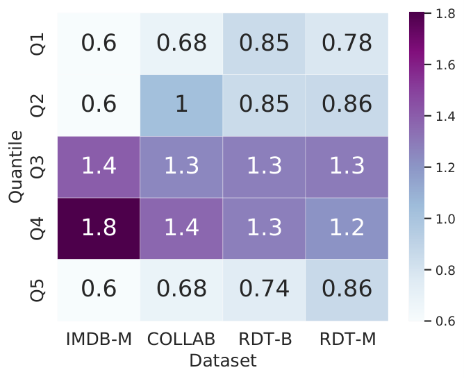
Performance variations due to spectral properties. We split the test graphs into quintiles based on their values to explore whether the test graph spectrum impacts the performance of the proposed augmentation process. Figure 5 displays the improvements obtained for each quintile. As suggested by our theoretical analysis in Section 4.5, we see a marked elevation for the middle quintiles of . These results support the conjecture that small or large values of (an approximation of in Section 4.5) adversely affect the embedding quality and the crop augmentation.
6 Conclusion
We introduce SGCL, a comprehensive suite of spectral augmentation methods suited to pre-training graph neural networks contrastively over large scale pre-train datasets. The proposed methods do not require labels or attributes, being reliant only on structure, and thus are applicable to a wide variety of settings. We show that our designed augmentations can aid the pre-training procedure to capture generalizable structural properties that are agnostic to downstream tasks. Our designs are not ad hoc, but are well motivated through spectral analysis of the graph and its connections to augmentations and other techniques in the domains of vision and network embedding analysis. The proposed augmentations make the graph encoder — trained by either E2E or MoCo — able to adapt to new datasets without fine-tuning. The suite outperforms the previous state-of-the-art methods with statistical significance. The observed improvements persist across multiple datasets for the three tasks of node classification, graph classification and similarity search.
References
- Belkin and Niyogi (2001) M. Belkin and P. Niyogi. Laplacian eigenmaps and spectral techniques for embedding and clustering. In Proc. Advances in Neural Information Processing Systems, 2001.
- Brouwer and Haemers (2011) A. E. Brouwer and W. H. Haemers. Spectra of graphs. Springer Science & Business Media, 2011.
- Chanpuriya and Musco (2020) S. Chanpuriya and C. Musco. Infinitewalk: Deep network embeddings as laplacian embeddings with a nonlinearity. In Proc. ACM SIGKDD Int. Conf. Knowledge Discovery & Data Mining, 2020.
- Chen et al. (2020a) M. Chen, Z. Wei, Z. Huang, B. Ding, and Y. Li. Simple and deep graph convolutional networks. In Proc. Int. Conf. Machine Learning, 2020a.
- Chen et al. (2020b) T. Chen, S. Kornblith, M. Norouzi, and G. Hinton. A simple framework for contrastive learning of visual representations. In Proc. Int. Conf. Machine Learning, 2020b.
- Chen et al. (2020c) X. Chen, M. Heimann, F. Vahedian, and D. Koutra. Cone-align: Consistent network alignment with proximity-preserving node embedding. In Proc. ACM SIGKDD Int. Conf. Knowledge Discovery & Data Mining, pages 1985–1988, 2020c.
- Chu et al. (2021) G. Chu, X. Wang, C. Shi, and X. Jiang. Cuco: Graph representation with curriculum contrastive learning. In Proc. Int. Joint Conf. Artificial Intelligence, 2021.
- Chung (1997) F. R. Chung. Spectral graph theory, volume 92. American Mathematical Soc., 1997.
- Chung and Graham (1997) F. R. Chung and F. C. Graham. Spectral graph theory. American Mathematical Soc., 1997.
- Davies et al. (2000) E. B. Davies, J. Leydold, and P. F. Stadler. Discrete nodal domain theorems. arXiv preprint math/0009120, 2000.
- Demmel (1997) J. W. Demmel. Applied numerical linear algebra. SIAM, 1997.
- Donnat et al. (2018) C. Donnat, M. Zitnik, D. Hallac, and J. Leskovec. Learning structural node embeddings via diffusion wavelets. In Proc. ACM SIGKDD Int. Conf. Knowledge Discovery & Data Mining, pages 1320–1329, 2018.
- Dwivedi et al. (2020) V. P. Dwivedi, C. K. Joshi, T. Laurent, Y. Bengio, and X. Bresson. Benchmarking graph neural networks. arXiv preprint arXiv:2003.00982, 2020.
- Errica et al. (2020) F. Errica, M. Podda, D. Bacciu, and A. Micheli. A fair comparison of graph neural networks for graph classification. arXiv preprint arXiv:1912.09893, 2020.
- Fiedler (1973) M. Fiedler. Algebraic connectivity of graphs. Czechoslovak mathematical journal, 23(2):298–305, 1973.
- Gilmer et al. (2017) J. Gilmer, S. S. Schoenholz, P. F. Riley, O. Vinyals, and G. E. Dahl. Neural message passing for quantum chemistry. In Proc. Int. Conf. Machine Learning, 2017.
- Grave et al. (2019) E. Grave, A. Joulin, and Q. Berthet. Unsupervised alignment of embeddings with wasserstein procrustes. In The 22nd International Conference on Artificial Intelligence and Statistics, pages 1880–1890. PMLR, 2019.
- Grill et al. (2020) J.-B. Grill, F. Strub, F. Altché, C. Tallec, P. Richemond, E. Buchatskaya, C. Doersch, B. Avila Pires, Z. Guo, M. Gheshlaghi Azar, et al. Bootstrap your own latent-a new approach to self-supervised learning. In Proc. Advances in Neural Information Processing Systems, 2020.
- Grover and Leskovec (2016) A. Grover and J. Leskovec. node2vec: Scalable feature learning for networks. In Proc. ACM SIGKDD Int. Conf. Knowledge Discovery & Data Mining, 2016.
- Gutmann and Hyvärinen (2010) M. Gutmann and A. Hyvärinen. Noise-contrastive estimation: A new estimation principle for unnormalized statistical models. In Proceedings of the thirteenth international conference on artificial intelligence and statistics, pages 297–304, 2010.
- Gutmann and Hyvärinen (2012) M. U. Gutmann and A. Hyvärinen. Noise-contrastive estimation of unnormalized statistical models, with applications to natural image statistics. Journal of machine learning research, 13(2), 2012.
- Hamilton et al. (2017) W. Hamilton, Z. Ying, and J. Leskovec. Inductive representation learning on large graphs. In NeurIPS, pages 1024–1034, 2017.
- Han et al. (2022) X. Han, Z. Jiang, N. Liu, and X. Hu. G-mixup: Graph data augmentation for graph classification. arXiv preprint arXiv:2202.07179, 2022.
- Hassani and Khasahmadi (2020) K. Hassani and A. H. Khasahmadi. Contrastive multi-view representation learning on graphs. In Proc. Int. Conf. Machine Learning, 2020.
- He et al. (2020) K. He, H. Fan, Y. Wu, S. Xie, and R. Girshick. Momentum contrast for unsupervised visual representation learning. In CVPR, 2020.
- Heimann et al. (2018) M. Heimann, H. Shen, T. Safavi, and D. Koutra. REGAL: Representation learning-based graph alignment. In Proc. of CIKM, 2018.
- Henderson et al. (2012) K. Henderson, B. Gallagher, T. Eliassi-Rad, H. Tong, S. Basu, L. Akoglu, D. Koutra, C. Faloutsos, and L. Li. Rolx: structural role extraction & mining in large graphs. In Proc. ACM SIGKDD Int. Conf. Knowledge Discovery & Data Mining, 2012.
- Hjelm et al. (2018) R. D. Hjelm, A. Fedorov, S. Lavoie-Marchildon, K. Grewal, P. Bachman, A. Trischler, and Y. Bengio. Learning deep representations by mutual information estimation and maximization. arXiv preprint arXiv:1808.06670, 2018.
- Hou et al. (2022) Z. Hou, X. Liu, Y. Dong, C. Wang, J. Tang, et al. Graphmae: Self-supervised masked graph autoencoders. In Proc. ACM SIG Int. Conf. Knowledge Discovery & Data Mining, 2022.
- Hu et al. (2020a) W. Hu, M. Fey, M. Zitnik, Y. Dong, H. Ren, B. Liu, M. Catasta, and J. Leskovec. Open graph benchmark: Datasets for machine learning on graphs. In Proc. Advances in Neural Information Processing Systems, volume 33, pages 22118–22133, 2020a.
- Hu et al. (2020b) W. Hu, B. Liu, J. Gomes, M. Zitnik, P. Liang, V. Pande, and J. Leskovec. Strategies for pre-training graph neural networks. In Proc. Int. Conf. Learning Representations, 2020b.
- Hu et al. (2020c) Z. Hu, Y. Dong, K. Wang, K.-W. Chang, and Y. Sun. Gpt-gnn: Generative pre-training of graph neural networks. In Proc. ACM SIG Int. Conf. Knowledge Discovery & Data Mining, pages 1857–1867, 2020c.
- Kahale (1995) N. Kahale. Eigenvalues and expansion of regular graphs. Journal of the ACM (JACM), 42(5):1091–1106, 1995.
- Khosla et al. (2020) P. Khosla, P. Teterwak, C. Wang, A. Sarna, Y. Tian, P. Isola, A. Maschinot, C. Liu, and D. Krishnan. Supervised contrastive learning. In Proc. Advances in Neural Information Processing Systems, 2020.
- Kipf and Welling (2017) T. N. Kipf and M. Welling. Semi-supervised classification with graph convolutional networks. In Proc. Int. Conf. Learning Representations, 2017.
- Kondor and Lafferty (2002) R. I. Kondor and J. Lafferty. Diffusion kernels on graphs and other discrete structures. In Proc. Int. Conf. Machine Learning, 2002.
- Kwok et al. (2013) T. C. Kwok, L. C. Lau, Y. T. Lee, S. Oveis Gharan, and L. Trevisan. Improved cheeger’s inequality: Analysis of spectral partitioning algorithms through higher order spectral gap. In Proceedings of the forty-fifth annual ACM symposium on Theory of computing, pages 11–20, 2013.
- Lee et al. (2014) J. R. Lee, S. O. Gharan, and L. Trevisan. Multiway spectral partitioning and higher-order cheeger inequalities. Journal of the ACM (JACM), 61(6):1–30, 2014.
- Lee et al. (2022) N. Lee, J. Lee, and C. Park. Augmentation-free self-supervised learning on graphs. In AAAI, 2022.
- Li et al. (2021) H. Li, X. Wang, Z. Zhang, Z. Yuan, H. Li, and W. Zhu. Disentangled contrastive learning on graphs. In Proc. Advances in Neural Information Processing Systems, 2021.
- McKnight and Najab (2010) P. E. McKnight and J. Najab. Mann-whitney u test. The Corsini encyclopedia of psychology, pages 1–1, 2010.
- Morris et al. (2020) C. Morris, N. M. Kriege, F. Bause, K. Kersting, P. Mutzel, and M. Neumann. Tudataset: A collection of benchmark datasets for learning with graphs. arXiv preprint arXiv:2007.08663, 2020.
- Narayanan et al. (2017) A. Narayanan, M. Chandramohan, R. Venkatesan, L. Chen, Y. Liu, and S. Jaiswal. graph2vec: Learning distributed representations of graphs. arXiv preprint arXiv:1707.05005, 2017.
- Ortega et al. (2018) A. Ortega, P. Frossard, J. Kovačević, J. M. Moura, and P. Vandergheynst. Graph signal processing: Overview, challenges, and applications. Proceedings of the IEEE, 106(5):808–828, 2018.
- Page et al. (1999) L. Page, S. Brin, R. Motwani, and T. Winograd. The PageRank citation ranking: Bringing order to the web. Technical report, Stanford InfoLab, 1999.
- Palowitch et al. (2022) J. Palowitch, A. Tsitsulin, B. Mayer, and B. Perozzi. Graphworld: Fake graphs bring real insights for gnns. arXiv preprint arXiv:2203.00112, 2022.
- Perozzi et al. (2014) B. Perozzi, R. Al-Rfou, and S. Skiena. DeepWalk: Online learning of social representations. In Proc. ACM SIGKDD Int. Conf. Knowledge Discovery & Data Mining, 2014.
- Qin et al. (2020) K. K. Qin, F. D. Salim, Y. Ren, W. Shao, M. Heimann, and D. Koutra. G-crewe: Graph compression with embedding for network alignment. In Proc. ACM SIG Int. Conf. Knowledge Discovery & Data Mining, pages 1255–1264, 2020.
- Qiu et al. (2018) J. Qiu, Y. Dong, H. Ma, J. Li, K. Wang, and J. Tang. Network embedding as matrix factorization: Unifying deepwalk, line, pte, and node2vec. In WSDM ’18, 2018.
- Qiu et al. (2020) J. Qiu, Q. Chen, Y. Dong, J. Zhang, H. Yang, M. Ding, K. Wang, and J. Tang. Gcc: Graph contrastive coding for graph neural network pre-training. In Proc. ACM SIGKDD Int. Conf. Knowledge Discovery & Data Mining, 2020.
- Ribeiro et al. (2017) L. F. Ribeiro, P. H. Saverese, and D. R. Figueiredo. struc2vec: Learning node representations from structural identity. In Proc. ACM SIGKDD Int. Conf. Knowledge Discovery & Data Mining, 2017.
- Rohe et al. (2011) K. Rohe, S. Chatterjee, and B. Yu. Spectral clustering and the high-dimensional stochastic blockmodel. The Annals of Statistics, 39(4):1878–1915, 2011.
- Sarkar and Bickel (2015) P. Sarkar and P. J. Bickel. Role of normalization in spectral clustering for stochastic blockmodels. The Annals of Statistics, 43(3):962–990, 2015.
- Singh et al. (2007) R. Singh, J. Xu, and B. Berger. Pairwise global alignment of protein interaction networks by matching neighborhood topology. In Annual International Conference on Research in Computational Molecular Biology, 2007.
- Spielman (2007) D. A. Spielman. Spectral graph theory and its applications. In 48th Annual IEEE Symposium on Foundations of Computer Science (FOCS’07), pages 29–38. IEEE, 2007.
- Spielman and Srivastava (2008) D. A. Spielman and N. Srivastava. Graph sparsification by effective resistances. In Proceedings of the fortieth annual ACM symposium on Theory of computing, pages 563–568, 2008.
- Sun et al. (2019) F.-Y. Sun, J. Hoffman, V. Verma, and J. Tang. Infograph: Unsupervised and semi-supervised graph-level representation learning via mutual information maximization. In Proc. Int. Conf. Learning Representations, 2019.
- Tang et al. (2015) J. Tang, M. Qu, M. Wang, M. Zhang, J. Yan, and Q. Mei. LINE: Large-scale information network embedding. In WWW ’15, 2015.
- Tong et al. (2006) H. Tong, C. Faloutsos, and J.-Y. Pan. Fast random walk with restart and its applications. In ICDM ’06, pages 613–622. IEEE, 2006.
- Torres et al. (2020) L. Torres, K. S. Chan, and T. Eliassi-Rad. Glee: Geometric laplacian eigenmap embedding. Journal of Complex Networks, 8(2):cnaa007, 2020.
- Veličković et al. (2018) P. Veličković, G. Cucurull, A. Casanova, A. Romero, P. Lio, and Y. Bengio. Graph attention networks. In Proc. Int. Conf. Learning Representations, 2018.
- Velickovic et al. (2019) P. Velickovic, W. Fedus, W. L. Hamilton, P. Liò, Y. Bengio, and R. D. Hjelm. Deep graph infomax. In Proc. Int. Conf. Learning Representations, 2019.
- Von Luxburg (2007a) U. Von Luxburg. A tutorial on spectral clustering. Statistics and computing, 17(4):395–416, 2007a.
- Von Luxburg (2007b) U. Von Luxburg. A tutorial on spectral clustering. Statistics and computing, 17(4):395–416, 2007b.
- Vu (2007) V. H. Vu. Spectral norm of random matrices. Combinatorica, 27(6):721–736, 2007.
- Vu (2014) V. H. Vu. Modern Aspects of Random Matrix Theory, volume 72. American Mathematical Society, 2014.
- Wang et al. (2020) Y. Wang, W. Wang, Y. Liang, Y. Cai, and B. Hooi. Graphcrop: Subgraph cropping for graph classification. arXiv preprint arXiv:2009.10564, 2020.
- Weyl (1912) H. Weyl. Das asymptotische verteilungsgesetz der eigenwerte linearer partieller differentialgleichungen (mit einer anwendung auf die theorie der hohlraumstrahlung). Mathematische Annalen, 71(4):441–479, 1912.
- Woolson (2007) R. F. Woolson. Wilcoxon signed-rank test. Wiley encyclopedia of clinical trials, pages 1–3, 2007.
- Wu et al. (2019) F. Wu, A. Souza, T. Zhang, C. Fifty, T. Yu, and K. Weinberger. Simplifying graph convolutional networks. In Proc. Int. Conf. Machine Learning, 2019.
- Xu et al. (2021) D. Xu, W. Cheng, D. Luo, H. Chen, and X. Zhang. InfoGCL: Information-aware graph contrastive learning. In Proc. Advances in Neural Information Processing Systems, 2021.
- Xu et al. (2019) K. Xu, W. Hu, J. Leskovec, and S. Jegelka. How powerful are graph neural networks? In Proc. Int. Conf. Learning Representations, 2019.
- Yanardag and Vishwanathan (2015) P. Yanardag and S. Vishwanathan. Deep graph kernels. In Proc. ACM SIGKDD Int. Conf. Knowledge Discovery & Data Mining, 2015.
- Yehudai et al. (2021) G. Yehudai, E. Fetaya, E. Meirom, G. Chechik, and H. Maron. From local structures to size generalization in graph neural networks. In Proc. Int. Conf. Machine Learning, pages 11975–11986. PMLR, 2021.
- Ying et al. (2018) Z. Ying, J. You, C. Morris, X. Ren, W. Hamilton, and J. Leskovec. Hierarchical graph representation learning with differentiable pooling. In Proc. Advances in Neural Information Processing Systems, 2018.
- You et al. (2020) Y. You, T. Chen, Y. Sui, T. Chen, Z. Wang, and Y. Shen. Graph contrastive learning with augmentations. In Proc. Advances in Neural Information Processing Systems, 2020.
- You et al. (2021) Y. You, T. Chen, Y. Shen, and Z. Wang. Graph contrastive learning automated. In Proc. Int. Conf. Machine Learning, pages 12121–12132. PMLR, 2021.
- You et al. (2022) Y. You, T. Chen, Z. Wang, and Y. Shen. Bringing your own view: Graph contrastive learning without prefabricated data augmentations. In WSDM, 2022.
- Zhang et al. (2019a) F. Zhang, X. Liu, J. Tang, Y. Dong, P. Yao, J. Zhang, X. Gu, Y. Wang, B. Shao, R. Li, et al. OAG: Toward linking large-scale heterogeneous entity graphs. In KDD, pages 2585–2595, 2019a.
- Zhang et al. (2015) J. Zhang, J. Tang, C. Ma, H. Tong, Y. Jing, and J. Li. Panther: Fast top-k similarity search on large networks. In Proc. ACM SIGKDD Int. Conf. Knowledge Discovery & Data Mining, 2015.
- Zhang et al. (2018) J. Zhang, X. Shi, J. Xie, H. Ma, I. King, and D.-Y. Yeung. Gaan: Gated attention networks for learning on large and spatiotemporal graphs. arXiv preprint arXiv:1803.07294, 2018.
- Zhang et al. (2019b) J. Zhang, Y. Dong, Y. Wang, and J. Tang. Prone: fast and scalable network representation learning. In Proc. Int. Joint Conf. Artificial Intelligence, pages 4278–4284, 2019b.
- Zhang et al. (2020) S. Zhang, Z. Hu, A. Subramonian, and Y. Sun. Motif-driven contrastive learning of graph representations. arXiv preprint arXiv:2012.12533, 2020.
- Zhu et al. (2020) Y. Zhu, Y. Xu, F. Yu, Q. Liu, S. Wu, and L. Wang. Deep graph contrastive representation learning. arXiv preprint arXiv:2006.04131, 2020.
- Zhu et al. (2021) Y. Zhu, Y. Xu, F. Yu, Q. Liu, S. Wu, and L. Wang. Graph contrastive learning with adaptive augmentation. In WWW, 2021.
Supplementary Materials for SGCL
List of all contents
- •
Sections to position our work better and provide references.
- •
Section has implementation details, ablations, statistical tests, and all other results not in the main text. Section adds confidence intervals and some more results and confidence intervals.
- •
Section has some results for MNIST and CIFAR-10 to illustrate linkages between our method and image cropping.
- •
Section discusses limitations, societal impact and reproducibility.
- •
Section has additional ablations based on spectral properties.
- •
Section has proofs of some mathematical results used in the paper for various augmentations.
- •
Section has proofs on the stochastic block model.
- •
Sections add small details that help explain how the entire suite works. Section has time complexity graphs, section has a case of negative transfer which pops up in some experiments and looks anomalous otherwise, and section visualizes why we need to align two graphs in the first place.
7 Position of our work
We emphasize that there are three distinct cases of consideration in the field of contrastive learning in graphs. We hope to make a clear separation between them to help readers understand our model design and the choice of baselines as well as the datasets we conduct experiments on. A summarizing of the position of our work vs. prior works is presented in Table 5.
|
|
|
|
| |||||||||||||||
|
|
|
|||||||||||||||||
|
Ours,GCC | Ours,GCC |
|
|
|
First, we have out of domain pre-training, where the encoder only sees a large pre-training corpus in the training phase that may share no node attributes at all with the downstream task. A representative method is GCC (Qiu et al. 2020). For example, this pre-training dataset can be a large citation network or social network (as the pre-train corpus used in our paper), while the downstream task may be on a completely different domain such as molecules. Since no node attributes are shared between the two domains, the initial node attributes have to rely solely on structure, e.g., the adjacency or Laplacian matrices and embeddings derived from their eigendecomposition . Importantly, in this case, the encoder is never trained on any labeled or unlabeled instances for the downstream graph related tasks before doing the inference. It allows the model to obtain the results on the downstream task very fast (since only the model inference step is applied to obtain the node representations for the downstream tasks). We call this setting pre-training with frozen encoder (out of domain). This is the most difficult graph contrastive learning (GCL) related task. In our paper, we strictly follow this setup. The downstream task performance can be further improved if the downstream training instances (data, but also possibly with labels) are shown to the GNN encoder. We call this setting pre-training with fine-tuning (out of domain).
Second, we have the domain specific pre-training method where the encoder sees a large pre-training corpus which shares similar features or the same feature tokenization method as the downstream task. The representative methods that fall under this category include GPT-GNN Hu et al. 2020c, GraphCL (You et al. 2020), MICRO-Graph (Zhang et al. 2020), JOAO (You et al. 2021), BYOV (You et al. 2022), and GraphMAE (Hou et al. 2022). The typical experiment design for this setting is to pre-train the GNN encoder on a large-scale bioinformatics dataset, and then fine-tune and evaluate on smaller datasets of the same category. Since the feature space is properly aligned between the pre-train dataset and the downstream datasets, the node attributes usually are fully exploited during the pre-training stage. Similarly, the downstream task performance can be further improved if the downstream tasks (data and/or their labels) are shown to the GNN encoder. We call these two setting pre-training with frozen encoder (same domain) and pre-training with encoder fine-tuning (same domain).
Third, in the unsupervised learning setting for GCL, there is no large pre-training corpus that is distinct from the downstream task data. Rather, the large training set of the downstream task is the sole material for contrastive pre-training. Note that in this case, if there are multiple unrelated downstream tasks, e.g., a citation network and also a molecule task, a separate pre-training procedure must be conducted for each task and a separate network must be trained. The representative methods that fall under this category include InfoGCL (Xu et al. 2021), MVGRL (Hassani and Khasahmadi 2020), GraphCL (You et al. 2020), GCA (Zhu et al. 2021). Generally speaking, for tasks that rely heavily on the node attributes (such as citations, and molecule graphs), such unsupervised methods, when the training set data (adjacency matrix and node attributes) is available for the unsupervised training phase, can potentially outperform the out of domain pre-trained frozen encoder case. But this is natural, and expected, because in the out-of-domain pre-training with a frozen encoder setting the pre-trained network never even sees the source domain. It can never take advantage of node attributes because the pre-train datasets do not share the same feature space as the downstream task. It can only rely on the potential transferable structural features. But this is also not its purpose - its purpose is to act like a general large language model (LLM) or a Foundation Model like GPT-3. Such a model is not necessarily an expert in every area and can be outperformed by, for instance, specific question-answer-specialized language models for answering questions, but it performs relatively well zero-shot in most tasks without needing any pre-training. This is why in our main paper, we did not compare with the commonly used small-scale datasets (Cora, Citesser) for the unsupervised learning tasks.
Previous papers in this field such as GraphMAE (Hou et al. 2022) often include the frozen, pre-trained models under the unsupervised category in the experiments, which is not completely accurate or fair. In fact, this category is relatively understudied and introduces unique challenges for the out-of-domain transfer setting. Its importance, and relative lack of study, is precisely why it deserves attention - it is a step toward out-of-domain generalization on graphs and avoids expensive pre-training in every domain. In the following table, we provide a novel way to categorize the existing graph contrastive learning work and we hope it provides better insight to the readers in terms of the position of our work.
Please note that even though not directly applicable for the pre-train (out of domain) mode, for the existing methods under the category of pre-train (same domain) and unsupervised learning, we are able to make modifications to allow them to be applied in the out of domain settings. The main changes are 1) we use the pre-train out of domain corpus to train the GNN encoder instead of ; 2) since the feature space between the pre-train domains and the target domain are not aligned, we use instead of the original feature X. We conduct the above modification to some of the existing unsupervised learning based methods such as MVGRL (Hassani and Khasahmadi 2020) and GraphCL (You et al. 2020). This is also why we cannot, without running the out of domain pre-training experiment setups, directly report the experimental performance in the previous papers (largely unsupervised, except GCC), and why some of our numbers do not always agree with those reported in the original paper, e.g., MVGRL on IMDB-BINARY. The entire training process is completely different with a new pre-training corpus, and the same numbers are not guaranteed to occur.
8 Reasons to pursue augmentations based on graph spectra
First, we want to address the question of what is meant by the term "universal topological properties". Our method is inherently focused on transferring the pre-trained GNN encoder to any domain of graphs, including those that share no node attributes with the pre-train data corpus. This means that the only properties the encoder can use when building its representation are transferable structural clues. We use the word topological to denote this structure-only learning. The word universal denotes the idea of being able to easily transfer from pre-train graphs to any downstream graphs. It is a common practice to augment node descriptors with structural features (Errica et al. 2020), especially for graph classification tasks. DiffPool (Ying et al. 2018) adds the degree and clustering coefficient to each node feature vector. GIN (Xu et al. 2019) adds a one-hot representation of node degrees. In short, a universal topological property is some property such as the human-defined property of "degree" that we hope the GNN will learn in an unsupervised fashion. Just as degree - a very useful attribute to know for any graph for many downstream tasks - is derivable from the adjacency matrix by taking a row sum, we hope the GNN will learn a sequence of operations that distill some concept that is even more meaningful than the degree and other basic graph statistics.
Since structural clues are the only ones that can be transferable between pre-train graphs and the downstream graphs, the next part to answer is why spectral methods, and why should we use the spectral-inspired augmentations to achieve the out-of-domain generalization goal. We elaborate as follows.
For multiple decades, researchers have demonstrated the success of graph spectral signals with respect to preserving the unique structural characteristics of graphs (see (Torres et al. 2020) and references therein). Graph spectral analysis has also been the subject of extensive theoretical study and it has been established that the graph spectral information is important to characterize the graph properties. For example, graph spectral values (such as the Fiedler eigenvalue) related directly to fundamental properties such as graph partitioning properties (Kwok et al. 2013; Lee et al. 2014) and graph connectivity (Chung 1997; Kahale 1995; Fiedler 1973). Spectral analyses of the Laplacian matrix have well-established applications in graph theory, network science, graph mining, and dimensionality reduction for graphs (Torres et al. 2020). They have also been used for important tasks such as clustering (Belkin and Niyogi 2001; Von Luxburg 2007b) and sparsification (Spielman and Srivastava 2008). Moreover, many network embedding methods such as LINE (Tang et al. 2015) and DeepWalk reduce to factorizing a matrix derived from the Laplacian, as addressed in NetMF (Qiu et al. 2018). These graph spectral clues allow us to extract transferable structural features and structural commonality across graphs from different domains. All of these considerations motivate us to use spectral-inspired augmentations for graph contrastive learning to fully exploit the potential universal topological properties across graphs from different domains.
9 Related Work Extension
9.1 Representation learning on graphs
A significant body of research focuses on using graph neural networks to encode both the underlying graph describing relationships between nodes as well as the attributes for each node (Kipf and Welling 2017; Gilmer et al. 2017; Hamilton et al. 2017; Veličković et al. 2018; Xu et al. 2019). The core idea for GNNs is to perform feature mapping and recursive neighborhood aggregation based on the local neighborhood using shared aggregation functions. The neighborhood feature mapping and aggregation steps can be parameterized by learnable weights, which together constitute the graph encoder.
There has been a rich vein of literature that discusses how to design an effective graph encoding function that can leverage both node attributes and structure information to learn representations (Kipf and Welling 2017; Hamilton et al. 2017; Veličković et al. 2018; Zhang et al. 2018; Wu et al. 2019; Chen et al. 2020a; Xu et al. 2019). In particular, we highlight the Graph Isomorphism Network (GIN) (Xu et al. 2019), which is an architecture that is provably one of the most expressive among the class of GNNs and is as powerful as the Weisfeiler Lehman graph isomorphism test. Graph encoding is a crucial component of GNN pre-training and self-supervised learning methods. However, most existing graph encoders are based on message passing and the transformation of the initial node attributes. Such encoders can only capture vertex similarity based on features or node proximity, and are thus restricted to being domain-specific, incapable of achieving transfer to unseen or out-of-distribution graphs. In this work, to circumvent this issue, we employ structural positional encoding to construct the initial node attributes. By focusing on each node’s local subgraph level representation, we can extract universal topological properties that apply across multiple graphs. This endows the resultant graph encoder with the potential to achieve out-of-domain graph data transfer.
9.2 Data augmentations for contrastive learning
Augmentations for image data.
Representation learning is of perennial importance in machine learning with contrastive learning being a recent prominent technique. In the field of representation learning for image data, under this framework, there has been an active research theme in terms of defining a set of transformations applied to image samples, which do not change the semantics of the image. Candidate transformations include cropping, resizing, Gaussian blur, rotation, and color distortion. Recent experimental studies (Chen et al. 2020b; Grill et al. 2020) have highlighted that the combination of random crop and color distortion can lead to significantly improved performance for image contrastive learning. Inspired by this observation, we seek analogous graph augmentations.
Augmentations for graph data.
The unique nature of graph data means that the augmentation strategy plays a key role in the success of graph contrastive learning (Qiu et al. 2020; You et al. 2020; Li et al. 2021; Sun et al. 2019; Hassani and Khasahmadi 2020; Xu et al. 2021). Commonly-used graph augmentations include: 1) attribute dropping or masking (You et al. 2020; Hu et al. 2020c): these graph feature augmentations rely heavily on domain knowledge and this prevents learning a domain invariant encoder that can transfer to out-of-domain downstream tasks; 2) random edge/node dropping (Li et al. 2021; Xu et al. 2021; Zhu et al. 2020; Zhu et al. 2021): these augmentations are based on heuristics and they are not tailored to preserve any special graph properties; 3) graph diffusion (Hassani and Khasahmadi 2020): this operation offers a novel way to generate positive samples, but it has a large additional computation cost (Hassani and Khasahmadi 2020; Page et al. 1999; Kondor and Lafferty 2002). The graph diffusion operation is more costly than calculation and application of the Personalized Page Rank (PPR) (Page et al. 1999) based transition matrix since it requires an inversion of the adjacency matrix; and 4) random walks around a center node (Tong et al. 2006; Qiu et al. 2020): this augmentation creates two independent random walks from each vertex that explore its ego network and these form multiple views (subgraphs) of each node. Additionally, there is an augmentation called GraphCrop (Wang et al. 2020), which uses a node-centric strategy to crop a contiguous subgraph from the original graph while maintaining its connectivity; this is different from the spectral graph cropping we propose. Existing structure augmentation strategies are not tailored to any special graph properties and might unexpectedly change the semantics (Lee et al. 2022).
9.3 Pre-training, self-supervision, unsupervised & contrastive graph representation learning
Though not identical, pre-training, self-supervised learning, and contrastive learning approaches in the graph learning domain use many of the same underlying methods. A simple technique such as attribute masking can, for example, be used in pre-training as a surrogate task of predicting the masked attribute, while in the contrastive learning scenario, the masking is treated as an augmentation. We categorize the existing work into the following 5 categories.
| Approaches | Goal is pre-training or transfer | No requirement for features | Domain transfer | Shareable graph encoder |
| Category 1 (DGI, InfoGraph, MVGRL, DGCL, InfoGCL, AFGRL) | ✗ | ✗ | ✗ | ✗ |
| Category 2 (GPT-GNN, Strategies for pre-training GNNs) | ✔ | ✗ | ✗ | ✔ |
| Category 3 (Deepwalk, LINE, node2vec) | ✗ | ✔ | ✔ | ✗ |
| Category 4 (struc2vec, graph2vec, DGK, Graphwave, InfiniteWalk) | ✗ | ✔ | ✔ | ✗ |
| Category 5 (GraphCL, CuCo⋆, GCC, BYOV, GRACE⋆, GCA⋆, Ours) | ✔ | ✔ | ✔ | ✔ |
Category 1.
One of the early works in the contrastive graph learning direction is Deep Graph Infomax (DGI) (Velickovic et al. 2019). Though not formally identified as contrastive learning, the method aims to maximize the mutual information between the patch-level and high-level summaries of a graph, which may be thought of as two views. Infomax is a similar method that uses a GIN (Graph Isomorphism Network) and avoids the costly negative sampling by using batch-wise generation (Sun et al. 2019). MVGRL (Hassani and Khasahmadi 2020) tackles the case of multiple views, i.e., positive pairs per instance, similar to Contrastive Multiview coding for images. DGCL (Li et al. 2021) adopts a disentanglement approach, ensuring that the representation can be factored into components that capture distinct aspects of the graph. InfoGCL (Xu et al. 2021) learns representations using the Information Bottleneck (IB) to ensure that the views minimize overlapping information while preserving as much label-relevant information as possible. None of the methods in this category is capable of capturing universal topological properties that extend across multiple graphs from different domains.
Category 2.
Predicting masked edges/attributes in chemical and biological contexts has emerged as a successful pre-train task. GPT-GNN (Hu et al. 2020c) performs generative pre-training successively over the graph structure and relevant attributes. In (Hu et al. 2020b), Hu et al. propose several strategies (attribute masking, context structure prediction) to pre-train GNNs with joint node-level and graph-level contrastive objectives. This allows the model to better encode domain-specific knowledge. However, the predictive task for these methods relies heavily on the features and domain knowledge. As a result, the methods are not easily applied to general graph learning problems.
Category 3
Random-walk-based embedding methods like Deepwalk (Perozzi et al. 2014), LINE (Tang et al. 2015), and Node2vec (Grover and Leskovec 2016) are widely used to learn network embeddings in an unsupervised way. The main purpose is to encode the similarity by measuring the proximity between nodes. The embeddings are derived from the skip-gram encoding method, Word2vec, in Natural Language Processing (NLP). However, the proximity similarity information can only be applied within the same graph. Transfer to unseen graphs is challenging since the embeddings learned on different graphs are not naturally aligned.
Category 4
To aid transferring learned representations, another approach of unsupervised learning attempts encoding structural similarities. Two nodes can be structurally similar while belonging to two different graphs. Handcrafted domain knowledge based representative structural patterns are proposed in (Yanardag and Vishwanathan 2015; Ribeiro et al. 2017; Narayanan et al. 2017). Spectral graph theory provides the foundation for modelling structural similarity in (Qiu et al. 2018; Donnat et al. 2018; Chanpuriya and Musco 2020).
Category 5
In the domain of explicitly contrastive graph learning, we consider Graph Contrastive Coding (GCC) (Qiu et al. 2020) as the closest approach to our work. In GCC, the core augmentation used is random walk with return (Tong et al. 2006). This forms multiple views (subgraphs) of each node. GraphCL (You et al. 2020) expands this augmentation suite to add node dropping, edge perturbations, and attribute masking. Additionally, although they are not designed for pre-training, we integrated the augmentation strategies from MVGRL (Hassani and Khasahmadi 2020), Grace (Zhu et al. 2020), Cuco (Chu et al. 2021), and Bringing Your Own View (BYOV) (You et al. 2022) to work with the pre-train setup in category 5.
10 Implementation details, additional results, and ablations
10.1 Codebase references
In general, we follow the code base of GCC (Qiu et al. 2020), provided at : https://github.com/THUDM/GCC. We use it as a base for our own implementation (provided along with supplement). Please refer to it in general with this section. For results using struc2vec (Ribeiro et al. 2017), ProNE (Zhang et al. 2019b), Panther (Zhang et al. 2015), RolX (Henderson et al. 2012) and graphwave (Donnat et al. 2018) we report the results directly from (Qiu et al. 2020) wherever applicable.
10.2 Dataset details
We provide the important details of the pre-training datasets in the main paper, so here we describe the downstream datasets. We obtain US-airport from the core repository of GCC (Qiu et al. 2020) which itself obtains it from (Ribeiro et al. 2017). H-index is obtained from GCC as well via OAG (Zhang et al. 2019a). COLLAB, REDDIT-BINARY, REDDIT-MULTI5K, IMDB-BINARY, IMDB-MULTI all originally derive from the graph kernel benchmarks (Morris et al. 2020), provided at : https://chrsmrrs.github.io/datasets/. Finally, the top-k similarity datasets namely KDD-ICDM,SIGIR-CIKM,and SIGMOD-ICDE, are obtained from the GCC repository (Qiu et al. 2020); these were obtained from the original source, Panther (Zhang et al. 2015).
10.3 Hyperparameters and statistical experimental methodology
Hyperparameters: Training occurs over steps with a linear ramping-on (over the first ) and linear decay (over the last ) using the ADAM optimizer, with an initial learning rate of , . The random walk return probability is . The dictionary size , for MoCo . The batch size is for and for MoCo. The dropout is set to with a degree embedding of dimension and positional embedding of dimension . These hyperparameters are retained from GCC and do not require grid search. The hyperparameter for alignment is chosen by grid search from values, namely .
Runtime: Using DBLP as the test bed, we observed seconds per epoch for baseline GCC, which was only increased to at most seconds in the settings with the most augmentations. Note that epoch time is largely CPU controlled in our experience and may vary from server to server. However, we found that the ratios between different methods were far more stable. The main paper reports these values on a per graph basis.
Confidence intervals and statistical methodology
: To construct confidence bounds around our results, we carry out the following procedure. We introduce some randomness through seeds. The seed is employed twice: once during training the encoder, and again while fine-tuning the encoder on downstream tasks on the datasets. We carry out training with random seeds, resulting in encoders. From each of these encoders, the representation of the graphs in the downstream datasets is extracted.
Next, we train a SVC (for graph datasets) or a logistic regression module (for node datasets), both with a regularization co-efficient over stratified K-fold splits. Before testing the model obtained from the train fraction of any split, we sample uniformly with replacement from the test set of the split of size until we draw samples. These instances are graphs (ego-graphs for the case of node datasets and distinct graphs for the case of graph datasets). After this we report the testing result. This is a bootstrapping procedure that leads to a random re-weighing of test samples. This entire process - i.e., generating a new -fold split, training, bootstrapping, testing - is repeated times per encoder.
This leads to a total of data points per encoder, allowing fine-grained confidence intervals. However, we found that performance varied too strongly as a function of the splits, leading us to average over the splits instead. Therefore, each determination carries an effective sample size of . Upon this, the Whitney-Mann, Wilcoxon signed rank, and t-tests are carried out to determine p-values, to percentile confidence bounds, and standard deviations.
10.4 Augmentation details and sequences
Masking:
As mentioned in the main paper, we follow previous work (Hu et al. 2020b) and add simple masking of . The masking involves setting some columns to zero. Since we consider smaller eigenvalues of to be more important, we draw an integer uniformly in the range and mask out eigenvectors corresponding to the top eigenvalues of .
Sequence of augmentations:
We have discussed the creation of views of from graph instances . However, in our case, the goal is to create two positive views per mini-batch for an instance . Let us now clarify the sequence of augmentations we employ. It should be understood that for any , the negative view is any augmented or un-augmented view of .
- •
First, we create using random walk with return on . We use the random walk hyperparameters identified in (Qiu et al. 2020).
- •
With probability , we then test using similarity or diversity thresholds and repeat the first step if the test fails. If do not pass in tries, we proceed to the next step.
- •
We randomly crop both independently with probabilities over different crops (including no crop). In total, we allow five outcomes, i.e. . The last outcome is the case of no cropping. We keep , . These correspond to different types of crops, explained below. We can term as .
- •
With probability , we replace with or keep unchanged with probability .
- •
We apply one of the mask and reorder augmentations on both independently to form the final positive pairs. That is, for , we mask it with , or reorder it with , or keep it unchanged with . The same process is then done, independently, for .
For a graph , the values for cropping are chosen as follows. We calculate the values taken by the second eigenvector over and rank them, and set on the basis of the rank. That is, would correspond to being set as the -th percentile value over . This is done instead of absolute thresholds to sidestep the changes of the second eigenvector over the different s. The corresponding different types of crop are, written as values tuples :
- •
with
- •
with
- •
with
- •
with
- •
No crop, with
Note that in terms of alignment augmentations, our arguments regarding being transformed to as it respects the inner product carry over if we instead use or as the augmented views.
Order of augmentations. We have chosen the augmentations to proceed in this order due to the following reasons.
- •
Of all the candidates for the first augmentation in our sequence, the random walk is supreme as it cuts down on the size of the ego-net for the future steps and the Laplacian eigendecomposition’s complexity as well. Doing away with it greatly increases the runtime for any other step preceding it.
- •
Filtering is best done as early as possible to reject candidates on its basis before expensive augmentation steps have already been performed. Hence, we place it second.
- •
Cropping precedes align, mask and ordering as these change the attribute vectors, and cropping uses the second eigenvector which is part of the embedding itself.
- •
Alignment precedes mask and reorder, as alignment on shifted embeddings post-mask or post-reorder no longer follows from our arguments of its necessity.
- •
Mask and reorder are mutually exclusive as reordering a masked matrix does not obey the diffusion matrix argument we make for reordering as an augmentation. While masking a diffused matrix is logically allowed, we did not experiment on this case thoroughly and did not find any encouraging preliminary empirical results for this case.
We do not claim our order is the best of all possible permutations. Nevertheless, it can be seen the choice is not entirely ad hoc.
10.5 Ablation tables
The necessity of our spectral crop and reorder frequency components. We first report in Table 1 the results of ablations that involve replacing the proposed crop and reorder augmentations with random analogues. The results validate the necessity of following our eigenspectrum-designed approaches for cropping and reordering. We explore replacing the proposed crop with a random crop (randomly selecting a subgraph by excluding nodes). For reordering, we compare to a random permutation of spectral positional encoding. We observe a consistent drop in performance across all datasets when we replace either augmentation with its random counterpart. This indicates that our spectral augmentation designs can make a significant difference in terms of capturing more effective universal topological properties.
| Augment | US-Airport | H-index | IMDB-B | IMDB-M | COLLAB | RDT-B | RDT-M |
| GCC | 64.8 | 78.3 | 71.7 | 49.3 | 74.7 | 87.5 | 52.6 |
| SGCL - Random Permute | 63.5 | 76.1 | 71.4 | 47.8 | 74.2 | 86.8 | 52.2 |
| SGCL - Random Crop | 64.5 | 78.5 | 71.8 | 49.4 | 74.4 | 87.8 | 52.1 |
| SGCL | 65.3* | 78.9 | 73.0* | 49.8 | 75.6* | 88.4* | 53.8* |
In this section we now report the results for all other datasets when subjected to pairwise augmentations. We do want to re-iterate that since we have ten downstream datasets and five large-scale pre-train datasets, we select Reddit-binary as the downstream task and the smallest pre-train DBLP (SNAP) dataset as a demonstration. Using more pre-train datasets should result in further performance improvements, but due to computation time constraints, we focus on the simpler setting. We present these results (raw percentage gains over GCC) in tables 2,3,4,5,6,7,8. Statistically positive and negative cases are marked accordingly.
| Dataset | S-Crop | Mask | S-Reorder | Align | Similar | Diverse |
| S-Crop | 0.22 | 0.47 | 0.43 | 0.54 | 0.71 | -0.38 |
| Mask | 0.15 | 0.26 | 0.35 | 0.42 | -0.15 | |
| S-Reorder | 0.18 | 0.19 | 0.58 | 0.45 | ||
| Align | 0.16 | 0.56 | -0.26 | |||
| Similar | 0.31 | N/A | ||||
| Diverse | -0.72 |
| Dataset | Crop | Mask | Reorder | Align | Similar | Diverse |
| Crop | 0.62 | 0.58 | 0.55 | 0.43 | 0.85 | 0.32 |
| Mask | -0.24 | -0.56 | -1.04 | 0.52 | -0.17 | |
| Reorder | -0.14 | -0.49 | 0.38 | -0.26 | ||
| Align | -0.47 | 0.64 | -0.56 | |||
| Similar | 0.45 | N/A | ||||
| Diverse | -0.59 |
| Dataset | Crop | Mask | Reorder | Align | Similar | Diverse |
| Crop | 0.83 | 0.92 | 1.16 | 0.98 | 0.87 | 0.62 |
| Mask | -0.32 | 0.58 | 0.22 | -0.35 | -0.78 | |
| Reorder | 0.75 | 0.82 | 0.56 | 0.43 | ||
| Align | 0.18 | -0.19 | -0.22 | |||
| Similar | -0.08 | N/A | ||||
| Diverse | -0.15 |
| Dataset | Crop | Mask | Reorder | Align | Similar | Diverse |
| Crop | 0.24 | 0.42 | 0.56 | 0.47 | 0.38 | 0.31 |
| Mask | 0.31 | 0.52 | 0.43 | 0.25 | 0.38 | |
| Reorder | 0.48 | 0.38 | 0.21 | 0.34 | ||
| Align | 0.28 | 0.20 | 0.36 | |||
| Similar | -0.11 | N/A | ||||
| Diverse | 0.06 |
| Dataset | Crop | Mask | Reorder | Align | Similar | Diverse |
| Crop | -0.08 | 0.27 | -0.18 | -0.43 | 0.28 | 0.22 |
| Mask | 0.31 | 0.26 | 0.16 | 0.43 | 0.38 | |
| Reorder | -0.15 | -0.23 | -0.07 | 0.03 | ||
| Align | -0.12 | 0.14 | 0.05 | |||
| Similar | 0.25 | N/A | ||||
| Diverse | 0.14 |
| Dataset | Crop | Mask | Reorder | Align | Similar | Diverse |
| Crop | 0.23 | 0.42 | 0.32 | 0.34 | 0.71 | 0.54 |
| Mask | 0.18 | 0.45 | 0.32 | 0.62 | 0.42 | |
| Reorder | 0.22 | 0.45 | 0.55 | 0.59 | ||
| Align | 0.15 | 0.68 | 0.52 | |||
| Similar | 0.48 | N/A | ||||
| Diverse | 0.34 |
| Dataset | Crop | Mask | Reorder | Align | Similar | Diverse |
| Crop | 0.35 | 0.25 | 0.48 | 0.21 | 0.57 | 0.66 |
| Mask | -0.07 | 0.22 | -0.19 | 0.22 | 0.47 | |
| Reorder | 0.28 | 0.17 | 0.38 | 0.82 | ||
| Align | -0.11 | 0.16 | 0.54 | |||
| Similar | 0.19 | N/A | ||||
| Diverse | 0.62 |
10.6 Additional results with MoCo and Fine-tuning
Pre-trained encoders fine-tuned using ADAM with epochs warmup and epochs ramp-down with a learning rate of are used for the fine-tuned case. These results appear in tables 9, 10 and 11. We present results for E2E and MoCo (He et al. 2020) in both the frozen and fine-tuned setting.
| US-Airport | H-index | |||
| 1,190 | 5,000 | |||
| 13,599 | 44,020 | |||
| Frozen-like methods | ||||
| ProNE | 62.3 | 69.1 | ||
| GraphWave | 60.2 | 70.3 | ||
| Struc2vec | 66.2 | Day | ||
| Frozen | ||||
| Training mode | MoCo | E2E | MoCo | E2E |
| GCC | 65.6 | 64.8 | 75.2 | 78.3 |
| GraphCL | ||||
| GRACE | ||||
| MVGRL | ||||
| CuCo | ||||
| BYOV | ||||
| InfoGCL | ||||
| GCA | ||||
| SGCL | 76.7 | 78.9* | ||
| Fine-tuned | ||||
| Training mode | MoCo | E2E | MoCo | E2E |
| GCC | 67.2 | 68.3 | 80.6 | 80.5 |
| GraphCL | ||||
| GRACE | ||||
| MVGRL | ||||
| CuCo | ||||
| BYOV | ||||
| InfoGCL | ||||
| GCA | ||||
| SGCL | 67.5 | 68.6 | 80.8 | 80.7 |
| Datasets | IMDB-B | IMDB-M | COLLAB | RDT-B | RDT-M | |||||
| # graphs | 1,000 | 1,500 | 5,000 | 2,000 | 5,000 | |||||
| # classes | 2 | 3 | 3 | 2 | 5 | |||||
| Avg. # nodes | 19.8 | 13.0 | 74.5 | 429.6 | 508.5 | |||||
| Frozen-like methods | ||||||||||
| DGK | 67.0 | 44.6 | 73.1 | 78.0 | 41.3 | |||||
| graph2vec | 71.1 | 50.4 | – | 75.8 | 47.9 | |||||
| InfoGraph | 73.0 | 49.7 | – | 82.5 | 53.5 | |||||
| Frozen | ||||||||||
| Training mode | MoCo | E2E | MoCo | E2E | MoCo | E2E | MoCo | E2E | MoCo | E2E |
| GCC | 72.0 | 71.7 | 49.4 | 49.3 | 78.9 | 74.7 | 89.8 | 87.5 | 53.7 | 52.6 |
| GraphCL | ||||||||||
| GRACE | ||||||||||
| CuCo | 71.8 | 71.3 | 48.7 | 48.5 | 78.5 | 74.2 | 89.3 | 87.8 | 52.5 | 51.6 |
| BYOV | 72.3 | 72.0 | 48.5 | 49.2 | 78.4 | 75.1 | 89.5 | 87.9 | 53.6 | 53.0 |
| MVGRL | 72.3 | 72.2 | 49.2 | 49.4 | 78.6 | 75.0 | 89.6 | 87.4 | 53.4 | 52.8 |
| InfoGCL | 72.0 | 71.0 | 48.8 | 48.2 | 77.8 | 74.6 | 89.1 | 87.3 | 52.7 | 52.2 |
| GCA | 72.2 | 71.9 | 49.0 | 48.7 | 78.4 | 74.4 | 88.9 | 87.5 | 53.2 | 52.4 |
| SGCL | 73.4* | 73.0 | 79.7* | 75.6 | 90.6* | 88.4 | 54.2* | 53.8 | ||
| Fine-tuned | ||||||||||
| Training mode | MoCo | E2E | MoCo | E2E | MoCo | E2E | MoCo | E2E | MoCo | E2E |
| DGCNN | 70.0 | 47.8 | 73.7 | - | - | |||||
| GIN | 75.6* | 51.5* | 80.2 | 89.4* | 54.5 | |||||
| GCC(Random) | 75.6 | 50.9 | 79.4 | 87.8 | 52.1 | |||||
| GCC | 73.8 | 70.8 | 50.3 | 48.5 | 81.1 | 79.0 | 87.6 | 86.4 | 53.0 | 47.4 |
| GraphCL | ||||||||||
| GRACE | ||||||||||
| CuCo | 72.6 | 71.2 | 49.2 | 46.9 | 78.1 | 77.0 | 86.8 | 86.5 | 51.3 | 48.3 |
| BYOV | 73.5 | 72.4 | 50.1 | 49.6 | 81.2 | 79.3 | 88.2 | 87.0 | 53.9 | 50.2 |
| MVGRL | 72.3 | 72.2 | 49.2 | 49.4 | 78.6 | 77.3 | 87.9 | 86.8 | 53.4 | 49.8 |
| InfoGCL | 73.6 | 71.5 | 50.0 | 48.4 | 80.2 | 78.8 | 87.5 | 86.3 | 52.4 | 49.2 |
| GCA | 73.1 | 71.7 | 49.5 | 47.9 | 79.8 | 78.2 | 88.0 | 86.5 | 52.1 | 48.6 |
| SGCL | 81.5* | |||||||||
| KDD-ICDM | SIGIR-CIKM | SIGMOD-ICDE | ||||
| 2,867 | 2,607 | 2,851 | 3,548 | 2,616 | 2,559 | |
| 7,637 | 4,774 | 6,354 | 7,076 | 8,304 | 6,668 | |
| # ground truth | 697 | 874 | 898 | |||
| 20 | 40 | 20 | 40 | 20 | 40 | |
| Frozen-like methods | ||||||
| Random | 0.0198 | 0.0566 | 0.0223 | 0.0447 | 0.0221 | 0.0521 |
| RolX | 0.0779 | 0.1288 | 0.0548 | 0.0984 | 0.0776 | 0.1309 |
| Panther++ | 0.0892 | 0.1558 | 0.0782 | 0.1185 | 0.0921 | 0.1320 |
| GraphWave | 0.0846 | 0.1693 | 0.0549 | 0.0995 | 0.0947 | 0.1470 |
| E2E | ||||||
| GCC | 0.1047 | 0.1564 | 0.0549 | 0.1247 | 0.0835 | 0.1336 |
| GraphCL | 0.0986 | 0.1574 | 0.0583 | 0.1209 | 0.0796 | 0.1205 |
| GRACE | 0.1021 | 0.1558 | 0.0568 | 0.1226 | 0.0864 | 0.1262 |
| MVGRL | 0.0982 | 0.1483 | 0.0514 | 0.1174 | 0.0774 | 0.1159 |
| CuCo | 0.1063 | 0.1543 | 0.0568 | 0.1274 | 0.0924 | 0.1374 |
| BYOV | 0.1068 | 0.1585 | 0.0592 | 0.1268 | 0.0824 | 0.1318 |
| InfoGCL | 0.0972 | 0.1550 | 0.0595 | 0.1217 | 0.0802 | 0.1237 |
| GCA | 0.1007 | 0.1563 | 0.0559 | 0.1197 | 0.0849 | 0.1244 |
| SGCL | 0.1105* | 0.1642 | 0.0658 | 0.1363* | 0.1076* | 0.1561* |
| MoCo | ||||||
| GCC | 0.0904 | 0.1521 | 0.0652 | 0.1178 | 0.0846 | 0.1425 |
| GraphCL | 0.0835 | 0.1507 | 0.0629 | 0.1165 | 0.0872 | 0.1434 |
| GRACE | 0.0852 | 0.1516 | 0.0616 | 0.1172 | 0.0917 | 0.1469 |
| MVGRL | 0.0826 | 0.1458 | 0.0559 | 0.1116 | 0.0851 | 0.1387 |
| CuCo | 0.0864 | 0.1512 | 0.0624 | 0.1216 | 0.0877 | 0.1414 |
| BYOV | 0.0926 | 0.1553 | 0.0642 | 0.1228 | 0.0859 | 0.1468 |
| InfoGCL | 0.0848 | 0.1536 | 0.0619 | 0.1183 | 0.0884 | 0.1425 |
| GCA | 0.0843 | 0.1507 | 0.0607 | 0.1192 | 0.0865 | 0.1426 |
| SGCL | 0.0978* | 0.1627 | 0.0765 | 0.1306* | 0.1049* | 0.1583* |
10.7 Datasets and benchmark code
We obtain the datasets from the following sources :
- •
- •
- •
And the relevant benchmarks from :
- •
- •
GraphCL : https://github.com/Shen-Lab/GraphCL
- •
- •
- •
- •
11 Hardware details and statistical confidence intervals of results
Hardware and software: We tested all code on Python with PyTorch , CUDA , scikit-learn . The Tesla (one per model per run) served as the GPU.
We compute statistical confidence bounds only for the methods whose results we do not copy over from the GCC paper.
| US-Airport | H-index | |||
| 1,190 | 5,000 | |||
| 13,599 | 44,020 | |||
| Training mode | MoCo | E2E | MoCo | E2E |
| GraphCL | ||||
| GRACE | ||||
| MVGRL | ||||
| CuCo | ||||
| BYOV | ||||
| InfoGCL | ||||
| GCA | ||||
| SGCL | (0.2) | |||
| Fine-tuned | ||||
| Training mode | MoCo | E2E | MoCo | E2E |
| GraphCL | ||||
| GRACE | ||||
| MVGRL | ||||
| CuCo | ||||
| BYOV | ||||
| InfoGCL | ||||
| GCA | ||||
| SGCL | ||||
| Datasets | IMDB-B | IMDB-M | COLLAB | RDT-B | RDT-M | |||||
| # graphs | 1,000 | 1,500 | 5,000 | 2,000 | 5,000 | |||||
| # classes | 2 | 3 | 3 | 2 | 5 | |||||
| Avg. # nodes | 19.8 | 13.0 | 74.5 | 429.6 | 508.5 | |||||
| Frozen | ||||||||||
| Training mode | MoCo | E2E | MoCo | E2E | MoCo | E2E | MoCo | E2E | MoCo | E2E |
| GraphCL | (0.3) | |||||||||
| GRACE | ||||||||||
| CuCo | ||||||||||
| BYOV | ||||||||||
| MVGRL | ||||||||||
| InfoGCL | ||||||||||
| GCA | ||||||||||
| SGCL | ||||||||||
| Fine-tuned | ||||||||||
| Training mode | MoCo | E2E | MoCo | E2E | MoCo | E2E | MoCo | E2E | MoCo | E2E |
| GraphCL | ||||||||||
| GRACE | ||||||||||
| CuCo | ||||||||||
| BYOV | ||||||||||
| MVGRL | ||||||||||
| InfoGCL | ||||||||||
| GCA | ||||||||||
| SGCL | ||||||||||
| KDD-ICDM | SIGIR-CIKM | SIGMOD-ICDE | ||||
| 2,867 | 2,607 | 2,851 | 3,548 | 2,616 | 2,559 | |
| 7,637 | 4,774 | 6,354 | 7,076 | 8,304 | 6,668 | |
| # ground truth | 697 | 874 | 898 | |||
| 20 | 40 | 20 | 40 | 20 | 40 | |
| GraphCL | (0.0033) | (0.0016) | (0.0024) | ) | ||
| GRACE | (0.0037) | (0.0022) | (0.0041) | (0.0057) | (0.0012) | |
| MVGRL | (0.0028) | (0.0041) | (0.0038) | (0.0058) | (0.0062) | |
| CuCo | (0.0026) | (0.0031) | (0.0040) | (0.0038) | (0.0052) | (0.0081) |
| BYOV | (0.0019) | |||||
| InfoGCL | (0.0038) | |||||
| GCA | ||||||
| SGCL | (0.0024) | (0.0028) | (0.0042) | (0.0046) | (0.0028) | (0.0035) |
| MoCo | ||||||
| GraphCL | (0.0038) | (0.0031) | (0.0021) | (0.0021) | (0.0029) | |
| GRACE | (0.0026) | (0.0051) | ||||
| MVGRL | (0.0028) | (0.0037) | ||||
| CuCo | (0.0019) | (0.0052) | ||||
| BYOV | (0.0019) | (0.0027) | ||||
| InfoGCL | (0.0047) | (0.0038) | ||||
| GCA | ||||||
| SGCL | (0.0045) | (0.0041) | (0.0037) | (0.0029) | (0.0028) | (0.0031) |
12 Auxiliary experiments on OGB datasets, MNIST and CIFAR-10
12.1 MNIST and CIFAR-10 motivation - implicit assumptions for the crop augment
We now revisit the chain of reasoning that motivates the crop augmentation, enumerated below sequentially :
- •
Images are a very important, naturally occurring subclass of attributed grid graphs (products of line graphs). Indeed, for any grid graph, assigning the nodes a -dimensional attribute corresponding to the RGB intensity assigns the colour part of the image. For the spatial aspect, every grid graph is enumerable in the indices of its constituent line graphs that it is a product of, i.e. we may denote a node of the grid graph as where for a grid graph that is the product of two line graphs with nodes. Associate , with every such , with the condition that :
Clearly, then, every image can be expressed as a grid graph, while the converse is not true. We assume that this generalization is meaningful - after all, an image of shape can equally be flattened and written as a -dimensional sequence with its dimensions appended separately, yielding a length of per channel. Every image can be expressed this way while not every sequence of length can be formed into an image, making this a generalization. We need to demonstrate that the grid graph form of generalizing what an image is, turns out to be more meaningful via some metric than, for example, ad hoc flattening.
- •
The crop operation in images, when they are considered equivalent to grid graphs, is equivalent to a value-based thresholding on nodes, depending on the values induced on them using the first two eigenvectors corresponding to the first two nonzero eigenvalues of the Laplacian. This is indeed true, ignoring numerical errors in the eigendecomposition, when the dimensions with of the image are such that . However, the crop operation for images happens to be functional even when , which is not true for the eigenvector-based cropping we propose.
- •
The crop augment is known to be - practically and empirically - a runaway success among the candidate augmentations in contrastive learning so far, when the representations to be learnt are to be evaluated for image classification.
- •
Clearly, if the image is to be thought of as a graph, the corresponding expectation is that our proposed graph-level crop succeed for graph classification. Therefore, we investigate if value thresholding based on the two eigenvectors, which is strictly a generalization of the crop operation, is a similar success on graphs in general.
What are the questionable steps taken above ? First, using the first two eigenvectors is one of infinitely many generalizations possible of the crop augmentation. We cannot investigate all such generalizations, but we can instead check if this particular generalization continues to hold when the domain (images) is perturbed.
Secondly, to what extent is an image actually a grid graph ? Does such a generalization remove key aspects of the image ?
We can see that for the latter assumption, a start would be to consider the image classification tasks such as the ubiquitous tasks on MNIST and CIFAR-10, and turn them instead into graph classification tasks, after converting the images into grid graphs. If this process makes the task hopeless, the assumption is assuredly more questionable.
In fact, such benchmarking (Dwivedi et al. 2020) on MNIST and CIFAR-10 has already been carried out with Graph neural networks. The accuracy obtained is close to for MNIST, and above for CIFAR-10, which, while not exceptional, clearly shows that some reasonable information is retained relevant to the class labels by converting images to a grid graph.
Importantly, given such a grid graph, the nodes i.e. the pixels are initialized with their positions for such a graph classification task. We recall from our discussion of the spectra of grid graphs, that it is precisely the positions that will be recovered via the two relevant eigenvectors.
If our generalization is correct, then we expect that at the point of generalization - i.e. in the original domain, the generalization and the specific operation it is generalizing (crop) will be identical operations. We now need to change the domain as slightly as possible to the level where the generalization remains valid, but the specific operation can no longer be performed.
This is easily achievable by replacing images (grid graphs) with their subgraphs and assuming we have no clue how these graphs came to be (an usual assumption made for graph datasets). Recall that the positions to grid graphs were assigned using the knowledge that they were images. However, if we do not know that they are images, we can only use their adjacency matrices.
In the case of the complete grid graph, the adjacency matrix will be enough to recover the co-ordinates of each pixel. However, for a subgraph, the two eigenvectors induce different values that need not correlate to co-ordinates.
Recall that we have claimed that the values induced by these eigenvectors are useful for segmenting (selecting subgraphs from) graphs of arbitrary kinds for contrastive learning in the view creation process, using the images as an example. If they are useful for arbitrary graphs as our graph classification benchmarks indicate, they must be useful for slightly perturbed (transformed into subgraph) version of images. It should be understood that we are talking of usefulness solely in the sense of learning optimal representations for downstream classification tasks. If they cannot even succeed at this, then our reasoning is likely to be questionable.
Therefore, if the first two eigenvectors yield a positional encoding that is useful for the image classification task when the images are transformed into grid graphs and then made subgraphs of, the results will be consistent with our assumptions. Further, since the image has only meaningful co-ordinates upto axes, we expect no benefits for increasing the dimensionality of such spectral embeddings beyond .
Nature of testing
We consider the following cases, on top of a previously investigated baseline scenario, where each image is converted to a grid graph and each pixel to a node, with edges between adjacent pixels, and the node attribute is or dimensional respectively for MNIST and CIFAR-10, to which dimensions are added via the Laplacian decomposition’s eigenvectors corresponding to first two nonzero eigenvalues, bringing the problem into a graph classification problem, where a GCN (-layer GIN of the same architecture for consistency) is used to process this grid graph, and the node-level representations pooled.
The variants we investigate are :
- •
Keeping every graph as-is
- •
Replacing each graph with a subgraph, which consists of the nodes visited by a random walk starting from the center of each graph, taking steps with a return probability of
- •
Performing the subgraph step with a random graph crop on top of each subgraph, to simulate our augment scenario.
- •
Change the positional embedding to either be absent, have only the first dimension, or have dimensions.
In each of the following tables, namely tables 18, 18, 18, 18 for MNIST and 22, 22, 22, 22 for CIFAR-10, rows signify train sets, and columns signify test sets in terms of the modifications performed on them. Overall, we see the same pattern. The random walk, or the subsequent cropping, do not significantly harm the accuracy. There are large gains from going from -dimensional positional embeddings to , smaller ones from to and beyond , a significant drop at . This matches what we expect and justifies our assumptions.
| Original | Random Walk | Random Walk + Crop | |
| Original | 97.8 | 94.3 | 89.5 |
| Random Walk | 93.2 | 93.4 | 88.9 |
| Random Walk + Crop | 92.7 | 91.5 | 92.8 |
| Original | Random Walk | Random Walk + Crop | |
| Original | 94.2 | 87.4 | 85.6 |
| Random Walk | 86.5 | 85.1 | 83.5 |
| Random Walk + Crop | 83.2 | 81.2 | 85.9 |
| Original | Random Walk | Random Walk + Crop | |
| Original | 68.9 | 61.5 | 58.8 |
| Random Walk | 62.4 | 55.6 | 53.2 |
| Random Walk + Crop | 61.9 | 54.4 | 52.6 |
| Original | Random Walk | Random Walk + Crop | |
| Original | 95.6 | 93.2 | 87.2 |
| Random Walk | 91.5 | 84.2 | 84.5 |
| Random Walk + Crop | 91.9 | 86.5 | 83.8 |
| Original | Random Walk | Random Walk + Crop | |
| Original | 59.5 | 56.8 | 55.9 |
| Random Walk | 56.2 | 53.7 | 53.9 |
| Random Walk + Crop | 54.6 | 52.9 | 54.3 |
| Original | Random Walk | Random Walk + Crop | |
| Original | 55.4 | 49.7 | 52.3 |
| Random Walk | 54.2 | 51.2 | 50.8 |
| Random Walk + Crop | 53.2 | 47.8 | 53.2 |
| Original | Random Walk | Random Walk + Crop | |
| Original | 46.9 | 41.5 | 43.2 |
| Random Walk | 39.8 | 39.6 | 40.5 |
| Random Walk + Crop | 43.7 | 38.8 | 40.2 |
| Original | Random Walk | Random Walk + Crop | |
| Original | 52.7 | 51.0 | 53.5 |
| Random Walk | 52.4 | 49.6 | 51.0 |
| Random Walk + Crop | 51.3 | 50.5 | 50.2 |
12.2 Results on OGB datasets of Arxiv (accuracy) and molhiv (HIV) (ROC-AUC)
We also tested our pre-trained models on datasets associated with the Open Graph Benchmark aka OGB (Hu et al. 2020a). Here, the entire test occurs in the fine-tuned setting. We observed some mild benefits associated with pre-training over the common sense GIN benchmark, even when both networks had the advantage of utilizing the structural embedding (Recall, of course, that only the structural embedding aspect can transfer between widely divergent datasets that share no attributes otherwise). These results are summarized in table 23.
| Arxiv | HIV | |
| GIN - Attr + Struct | 72.1 | 77.0 |
| GIN - Attr only | 71.4 | 76.8 |
| GIN - Attr and Struct - GCC E2E Finetuned | 72.3 | 77.2 |
| GIN - Attr and Struct - GCC MoCo Finetuned | 72.3 | 77.5 |
| GIN - Attr and Struct - SGCL E2E Finetuned | 72.6 | 77.4 |
| GIN - Attr and Struct - SGCL MoCo Finetuned | 72.5 | 77.8 |
12.3 Citeseer and Cora
We ran the frozen E2E transfer case for Citeseer and Cora datasets. When we transferred our structure-only models to these datasets and did not use any node attributes, we observed 50.8 (1.6) and 68.7 (2.1) percent accuracy on Citeseer and Cora respectively (standard deviations in brackets).
With node features included along with the frozen encoder, the performance rose to 71.5 (1.2) and 82.1 (1.6) respectively. The fact that these values (50.8 and 68.7) are significantly higher than a random guess (approx. 14.3 and 16.7) indicates that the structure-only encoder trained on a completely different pre-training corpus is still able to learn important topological characteristics.
13 Limitations, societal impact and reproducibility
Limitations. Our paper is not without limitations. Currently, the pre-train datasets we use in our paper are mostly inherited from established work focusing on GNN pre-training (Qiu et al. 2020; You et al. 2020). Even though they are sufficiently large in terms of the scale of the graph, we believe our model can be further strengthened by more diverse graph datasets. As a very recent paper GraphWorld (Palowitch et al. 2022) addressed, the commonly used datasets have graph statistics that lie in a limited and sparsely-populated region in terms of metrics such as the clustering coefficient, degree distribution, or Gini coefficient. Thus, to fully benefit from the power of pre-training techniques for graph data, it would be interesting and important to extend the use of pre-train datasets to graphs with diverse structural properties.
Another limitation of our work is that the pre-training and transfer focuses exclusively on the graph structure information; this is a common approach for cross-domain training (Qiu et al. 2020). We believe that there is value in further investigation into techniques that can process the node feature information as well as the structure information during the pre-train stage. This especially can be seen with the OGB datasets, which may share structural information between, for example, molecules and citation networks, while sharing no attribute related information.
Potential societal impact. Graph neural network techniques have been commonly used for prediction tasks in social networks and recommender systems. Our techniques, as a variant of graph neural networks, can be used in those scenarios to further improve the model performance. However, having such an ability is a double-edged sword. On one hand, it can be beneficial to improve user experience. On the other hand, if these techniques are used purely for a profit-driven or political driven reason, they can aim to 1) monopolize user attention for as long as possible by seducing users into carrying out actions that will make them happy on very short timescales and addictive to their product or even worse to 2) shape and influence public opinion on the key matters of the time. Thus, researchers and service providers should pay vigilant attention to ensure the research does end up being used positively for the social good.
Reproducibility. We have included the code and all hyperparameters, hardware details etc. to facilitate reproducibility.
14 Additional ablations
In this section, we present the variation of the model’s success with changes in train dataset, degree, the standard deviation of the degree, and (the second eigenvalue of the Laplacian).
| Advantage | IMDB-M | COLLAB | RDT-B | RDT-M |
| All | 0.5(49.3) | 0.9(74.7) | 0.9(87.5) | 1.2(52.6) |
| LiveJournal | 0.4 (48.8) | 0.9 (74.2) | 1.0 (86.9) | 1.1 (51.8) |
| 0.5 (49.0) | 0.8 (74.0) | 1.0 (86.7) | 1.1 (51.6) | |
| IMDB | 0.6 (48.2) | 1.1 (73.8) | 1.1 (86.5) | 1.2 (51.5) |
| DBLP | 0.7 (49.1) | 1.1 (74.3) | 1.2 (86.4) | 1.1 (51.9) |
| Academia | 0.6 (48.1) | 1.0 (74.5) | 1.1 (86.2) | 1.1 (51.2) |
In the ablations against , degree, and standard deviation of the degree we see a pronounced U-curve where the middle quintiles perform best. This could be due to the hypothesized spectral gap effect that we derive. The results in degree statistics could well be due to the fact that such statistics in turn depend greatly on the values, and cannot be considered truly independent findings.
| Advantage | IMDB-M | COLLAB | RDT-B | RDT-M |
| Q1 | 0.3 (47.6) | 0.6 (74.2) | 0.8 (86.8) | 0.9 (51.6) |
| Q2 | 0.3 (48.7) | 0.9 (74.0) | 0.8 (86.7) | 1.0 (51.5) |
| Q3 | 0.7 (49.5) | 1.1 (74.9) | 1.2 (87.4) | 1.5 (52.3) |
| Q4 | 0.9 (49.4) | 1.2 (75.0) | 1.2 (88.0) | 1.4 (53.0) |
| Q5 | 0.3 (49.4) | 0.6 (74.9) | 0.7 (87.8) | 1.0 (52.9) |
| Advantage | IMDB-M | COLLAB | RDT-B | RDT-M |
| Q1 | 0.4 (48.6) | 0.7 (74.3) | 0.8 (87.4) | 1.0 (52.4) |
| Q2 | 0.5 (49.2) | 0.8 (74.5) | 1.0 (87.6) | 1.2 (52.5) |
| Q3 | 0.6 (49.0) | 1.0 (74.8) | 0.9 (87.2) | 1.3 (52.2) |
| Q4 | 0.5 (49.4) | 1.0 (74.6) | 1.0 (87.3) | 1.3 (52.4) |
| Q5 | 0.6 (49.3) | 1.1 (74.2) | 1.0 (87.6) | 1.3 (52.5) |
| Advantage | IMDB-M | COLLAB | RDT-B | RDT-M |
| Q1 | 0.5 (48.4) | 0.8 (74.3) | 0.8 (87.2) | 1.2 (52.9) |
| Q2 | 0.6 (49.5) | 0.9 (74.6) | 1.1 (87.6) | 1.3 (52.3) |
| Q3 | 0.6 (49.6) | 1.0 (75.0) | 1.2 (87.6) | 1.3 (52.4) |
| Q4 | 0.6 (50.0) | 1.1 (75.2) | 1.2 (87.7) | 1.3 (52.2) |
| Q5 | 0.3 (49.0) | 0.6 (74.2) | 0.7 (87.5) | 1.0 (52.2) |
| SGCL Accuracy | Q1 | Q2 | Q3 | Q4 | Q5 |
| Q1 | 73.8 | 73.5 | 73.6 | 73.4 | 73.2 |
| Q2 | 73.4 | 73.7 | 73.8 | 73.6 | 73.7 |
| Q3 | 73.8 | 74.2 | 74.2 | 74.1 | 74.0 |
| Q4 | 73.5 | 73.9 | 74.2 | 74.3 | 73.8 |
| Q5 | 73.3 | 73.2 | 73.7 | 73.6 | 73.6 |
15 Theorems underlying the augmentations
15.1 Crop augmentation
Let us derive a few key claims that will help us put the crop augment on a surer footing.
Denote by the path-graph on vertices, which has edges of form for . This corresponds to the line graph.
Define also , the ring graph on vertices defined as with an extra edge between and .
Recall the product graph : A product of two graphs with vertex sets and edge sets is a graph where each can be identified with an ordered pair . Two nodes corresponding to in have an edge between them if and only if either or . The product of two line graphs of length respectively can be represented as a planar rectangular grid of lengths . Denote by the rectangular grid graph formed by the product . Structurally, this graph represents an image with dimensions .
For simplicity, we will prove our work for unweighted and undirected graphs, but the properties are general and do not require these conditions.
Theorem 2
Let be a graph with eigenvalues of the Laplacian as and corresponding eigenvectors . Similarly consider another graph with eigenvalues and eigenvectors . Let the product of graphs be . Then, identifying each node in with an ordered pair , the Laplacian of has an eigenvector with eigenvalue , such that
Proof : let the laplacian of be . We need only compute the term
This is equivalent to (with being the edge set of respectively) :
However, taking , we observe that :
becomes, applying the hypothesized
Taking in common, we recognize that will yield just scaled by as is the eigenvector of the Laplacian.
Therefore this term becomes
While the other term, i.e.
yields similarly
Adding the two, we see that the final matrix-vector product is parallel to the original vector (thus an eigenvector) with eigenvalue .
Theorem 3
The eigenvectors of the (un-normalized) Laplacian of , for , are of the form:
with eigenvalues
.
Proof : We will use the ring graph defined above. Let be the path graph. is clearly the ring graph obtained by having two copies of with additional links.
Now, can be drawn on the plane with the vertex located at where . Observe that each vertex has a position in the plane which is parallel to the sum of the position vectors of and . From this, it naturally follows (by the definition of the Laplacian operator which subtracts the value of the neighbour vectors from that at the node) that the valid eigenvectors for are :
Regarding the eigenvalue, the node itself contributes (as it appears in the sum twice) and each neighbour contributes with neighbours, leading to an eigenvalue of .
Now it is trivial to find the eigenvectors of from . Simply take any eigenvector of which has the same value for for . Then the restriction of this eigenvector to defines a valid eigenvector for with the same eigenvalue. This is why the terms of the angles in the theorem are the same as path graphs with taking the place of as, for example
Which is the sought result.
15.2 Reordering augmentation
Theorem 4
Let be the adjacency matrix of an undirected unweighted graph, the degree matrix and the normalized adjacency matrix. Let be the -th order normalized diffusion matrix :
Then, the -th eigenvector (sorted in order of eigenvalues and ties broken consistently) is the same for all for any odd . That is, for any odd , and have eigenvectors ordered in the same sequence.
Proof : First, since the normalized Laplacian matrix is related to as , and it has eigenvalues in the range , has eigenvalues lying in the range .
Now, observe that shares the same eigenvectors with for any , however, eigenvalue changes to . It can be seen that since the permutation is on the basis of sorting eigenvalues, the view for will coincide with if is monotonic in the range , which is the range of allowed eigenvalues of the normalized adjacency matrix. It is trivial to note that is monotonically increasing for for any . Now, ignoring the case , observe that by the geometric progression formula. If is odd, is even, and thus is positive for . As we move from to the numerator monotonically rises, and the denominator monotonically falls from to , meaning that overall the function is monotonic and the ordering will just mirror . This is not true when the sum terminates at an even power, for instance, which is at and but negative at , indicating that it cannot be monotonic. The case where is or is trivially true.
15.3 Alignment closed forms
Given a function of the following nature where is orthogonal
Minimization of the above function can be done by noting that this is equivalent to working with :
, and we only have to maximize. This is , which is equal to . Maximizing this boils down to the projection of the matrix on the set of orthogonal matrices under the square Frobenius norm. Let the SVD of be , then we have being minimized. This becomes , with orthogonal and made to maximize inner product with diagonal , implying that is the solution.
16 Proofs on the stochastic block model
Usually, one divides graph contrastive learning and more generally all of contrastive learning into two categories :
- •
Supervised contrastive learning : There are unseen labels for each node. Our proofs will center on showing that with high probability, augmentations either preserve these unseen labels or some straightforward function of them that are made to suit the situation. For example, in a graph classification setting formed from the ego-graph of the nodes, the graph can be given the label of the node it is formed as an ego-graph from or the majority label of the nodes it contains. Our proofs in this case deal with the graph label and not the node label.
- •
Unsupervised graph contrastive learning : Each node is its own class (the classic setting of graph contrastive learning). In this scenario, it is not possible to work with the node label. Since in our setting, the nodes also possess no node-specific attributes beyond the structural information, our work here must focus on the structures obtained under spectral augmentation only.
In both cases we assume contrastive learning in general to work. That is, we show that the process of generating positive pairs etc. continues properly, but not anything about whether contrastive learning as a whole can generalize better or learn better representations. We view such a proof as outside the scope of this paper.
In the paper, we have worked with six distinct augmentations , of which two modify the structures chosen : Crop and Similar/Diverse. Three of them modify the attributes alone : Mask, reorder, and align. In general, nothing can be proven about the latter three without assuming an easy function class such as linear classifiers, which we view as unrealistic. Hence, our work focuses on the first two.
Secondly, we work with the stochastic block model and the two-cluster case where differing label of a node indicates a different propensity to create edges. We only focus on the case where there are seen or unseen labels which are related to the structure of graphs. This can be seen as a scenario intermediate between the supervised and unsupervised contrastive learning case, and the block model a natural reification to study it, for it is well known (Rohe et al. 2011) that conditional on the label of a node being known, the degree structure and density etc. strongly concentrate around their fixed values for the stochastic block model. Indeed, no other parameter except the label which directly determines the edge density even exists to provide information about the structure. Proving that nodes of similar (seen or unseen) labels are brought together by our augmentations carries over to the unsupervised case fully as these parameters are the only ones directly determining the structure.
By assuming that (unseen) labels exist, our proof is quite relevant to the actual use case of the paper. This is because in the downstream usage, the classifier is used, zero-shot, to provide representations that are used to predict the label. In other words, hidden latent labels are assumed to be predictable from the structure. Our case should be understood as a special case of unsupervised representation learning that shares some conditions with the supervised scenario.
16.1 Proof sketches and overall meaning
Our proofs center around the stochastic block model. In this setting the spectrum is well known and analyzed. We show that in this case, the “crop" operation around a node extracts a sub-graph of nodes which largely possess the same label as itself, where the label is considered to coincide with the cluster(block). Under the contrastive learning assumption, then, “crop" recovers positive pairs.
We also show that common embedding methods such as LINE, DeepWalk etc. are meaningful in terms of establishing “similar" and “diverse" views in the stochastic block model and that “similar" filtering would indeed yield a pathway to setting positive pairs apart. This is done by re-using our analysis for the supervised case which looks at the spectrum, and re-using the results from NETMF (Qiu et al. 2018) which connects the spectral results to embeddings obtained by random walks. In short, random walks and corresponding embeddings on stochastic block models can be seen, in the limit, as spectral decompositions of a block model with parameters that depend on the original block model. After this, we can recognize that the analysis for “crop", which essentially shows that the spectral embeddings form a meaningful metric of closeness in terms of label, cluster etc. on the original model, fully carries over with transformed parameters.
16.2 Supervised contrastive learning derivation
We define our stochastic block model (Rohe et al. 2011) as follows in keeping with conventions of the field. We will consider one with two components.
- •
There are nodes generated with label , and with label . Denote the group generated with label as and the other as . For simplicity, set
- •
An edge occurs with probability among two nodes of label , with probability between two nodes of label , and with among two nodes of different labels. is a common assumption. Without loss of generality we can take . We also consider the self-edges to be valid.
Note that in the setting of GCC, different local structures encode different labels. Hence , as if they were equal it would imply the same structural generation process gives rise to two different labels.
Let be the adjacency matrix of the stochastic block model and the laplacian. Let be the function that assigns to a node its value under the -th eigenvector of the Laplacian. Let be the cropped local neighbourhood around any node defined as where .
16.3 Factorizing the adjacency matrix
The overall matrix is of shape . Recall that we have allowed self-edges and diagonal entries of are not zero. Consider the matrix :
Let be a matrix formed by repeating the row vector times and then the row vector times. denotes the membership matrix. The first rows of denote that first nodes belong to label (and hence their zero-th entry is ) and the next rows likewise have a on their -nd column signifying that they have label .
Now, we can see that if we multiply , the first rows of the resulting matrix will be and the next will be . Consider now multiplying from the right side with i.e. forming, overall,. This matrix will be of shape and it can be seen that it has a block structure of form :
Where, is the vector of all -s, and the matrix of all -s. So, it can be seen that the above matrix is nothing but the expectation of the stochastic block model’s adjacency matrix.
Now, can we avoid analyzing this matrix and instead settle for analyzing the comparatively simpler ? Let be an eigenvector of with eigenvalue . Let have entries . By hypothesis, . Then, if we have the vector of shape with first entries as , and the next as
.
It can be seen that is parallel to an eigenvector of the expectation of the adjacency matrix and the corresponding eigenvalue is . However, we always assume eigenvectors are of unit norm, i.e. . So, is going to be not repeated times, but times and then times. This makes . Therefore, for every pair in the spectra of the matrix, there is a corresponding in the spectra of the expectation of the adjacency matrix. Next, note that the rank of the expectation of the adjacency is . So if the matrix has a full rank, there can be no extra eigenvalue-eigenvector pairs for the corresponding expectation of the adjacency matrix. All the nonzero eigenvalues and corresponding eigenvectors of the expectation of the adjacency are derivable from the matrix’s spectra. In short, to understand the spectrum of the expectation of adjacency, we can just study the matrix, as there is a one to one relationship between the nonzero eigenvalues and corresponding eigenvectors.
16.4 Crop augmentation
Notation of probability. In proofs involving convergence, it is customary to provide a guarantee that a statement holds with probability where tends to zero as goes to infinity. We will somewhat abuse the notation and say the probability as to denote this. We do not distinguish between things such as convergence in probability, convergence in distribution, almost surely convergence etc. and provide a largely concentration-inequality based proof overview.
We can state our proof for the crop augmentation as follows. All of the following statements hold with high probability (i.e. hold with a probability that as .)
Theorem 5
Let the number of samples . Let be chosen uniformly at random from the nodes. The following statements hold with a probability that as :
- •
Proposition 1 : The majority label in is the label of .
- •
Proposition 2 : Two nodes of different labels generate non-isomorphic cropped subgraphs , if is chosen uniformly at random as well.
- •
Proposition 3 : For any and , there is no differently labeled and which is isomorphic to for a high enough , if both are chosen uniformly at random.
Note that in the main text, we state a slightly different version of the theorem (Theorem of the main text) involving ego networks as well, which we restate here :
Theorem 6
Let node be chosen uniformly at random from , a -node graph generated according to the SBM described above. With probability for a function as , such that :
| (7) |
Terming used above as , we can see that this is adding an extra part that agrees with the node label, namely the majority label of an ego network. However, the majority label for the ego network when is trivially equal to the node’s label for at least some values of allowing beyond (i.e. the node itself is the ego network). To see this, take . The expected number of nodes of the same label - considering label for simplicity - in its ego network is , and the ones of a different label are of expected number . By Hoeffding’s inequality, both quantities with high probability i.e. with probability have deviations of only from their expectations which are terms of . Therefore, the majority label agrees with the node’s own label with high probability (note that this requires ). We assume this step to hold with high probability and focus now on proving the equality of the cropped subgraph’s majority label and the node label. We discuss ego networks other than the -ego network at the end of the section. It can be easily checked that at least for the -ego network, our proof involving mostly the vertex label case requires no changes.
To prove this, consider the random matrix . We can denote the expectation of as . We can see the rank of is as it has exactly 2 possible types of columns in it. It remains to find the corresponding two eigenvectors and eigenvalues. Clearly, by the structure of the matrix, the eigenvectors are of the form of repeating one value times and then another value times, and we can WLOG set and replace with . Then it remains to solve
Which becomes, by the definition of eigenvector,
or, simplifying :
Therefore, by the quadratic formula :
The eigenvalue for a corresponding is . Since the larger eigenvalue corresponds always to the larger value of . Therefore, takes the value gained by plugging in the negative root above, for c. This yields the unnormalized eigenvector, the actual entries assigned under the eigendecomposition are respectively when a vertex is assigned its value under the eigenvector.
We re-use previous results in random matrix theory (Vu 2007) (theorem ) that imply that with a probability , , when is . Since the lower bound on as we can assume it to hold for large . The notation denotes operator norm.
Explanation of the order through Hoeffding and RIP property. To intuitively understand the above result, we can consider each entry of . This is a random variable (blockwise) that takes one among the following set of values : (among the entries of label ), (among the entries between labels ) and (among label ). Now, only the upper triangle and diagonal are independent as the edges are symmetric, and the matrix is symmetric about the diagonal. We can write that :
Where, denotes Frobenius norm, and respectively denote summing over upper triangular and diagonal indices.
Therefore, if each entry of be denoted as , enumerated in any order over the diagonal and upper triangle of the matrix (), are independent r.v.s for any . Further, . Therefore, . Further, .
is a sum of independent random variables in a fixed, finite range of size . Therefore, Hoeffding’s inequality applies, which yields that with probability :
is the sum of the variances of random variables over entries, bounded above by . Hence, it follows that is with probability , therefore, is .
Further, we can see that has the following structure :
Where, are symmetric matrices with each upper triangular and diagonal entry as i.i.d random variables satisfying :
In addition, is a matrix (not necessarily symmetric) which has every entry as i.i.d realizations of such . Then, such a matrix by Restricted Isometry Property (Vu 2014) has the property that, with high probability, there is a constant independent of :
The left hand side is the maximum eigenvalue, which we recognize as i.e. the operator norm.
Now, using the relation between eigenvalues and the Frobenius norm :
The RHS comes from plugging in the Frobenius norm bound from the Hoeffding’s inequality step. Finally, this yields :
The result of Vu’s we state above is merely a formalization of this sketch with constants, the order is the same i.e. .
Now consider the second eigenvector i.e. the function from against the calculated above for . We need to use the Davis Kahan theorem (Demmel 1997) (theorem ) which states that if the angle between these is , then
As both eigenvectors are unit vectors, we can use the property that if two unit vectors have angle between them, the norm of their difference is bounded above by . Ignoring constants, we end up with the result that for some constant , and denoting the -th eigenvector of the Laplacian formed from some adjacency matrix
The LHS however works with the eigenvector of the overall adjacency matrix formed by the multiplication by we have discussed above. Recall that we have already noted the adjacency matrix and the matrix share eigenvalues upto scaling in . Their eigenvectors are also likewise related, and since eigenvectors are always of unit norm, an eigenvector of the matrix is first repeated in its entries and then normalized by a factor of by virtue of being an eigenvector, to become an eigenvector of the overall adjacency matrix.
By substituting the eigenvectors we found earlier, i.e. into the LHS, scaling by this factor cancels the extra on the RHS. Recalling that
Let :
Let be any pair of nodes that satisfy the conditions of :
- •
Labels of are different. WLOG, let have label , label .
- •
contains (and by symmetry, contains )
Clearly, we can see that either or . Let . Summing only over :
This yields a bound on , which we can term . Similarly, we can consider to get as : . Set to get :
Since we can term it . Simultaneously, consider :
Last inequality is by the property . By a similar argument as for , is of constant size and as . Let the maximum size of be . Now, if we pick a vertex of label at random, with probability , . If both these conditions hold, in any which does not have the same label must have . (Because any such pair must have at least one element in and ). Simultaneously, contains at least all vertices of label not in i.e. has vertices of label . Noting that values are all constants and implies that majority label in will agree with as completes the proof. The only aspect of the proof which required high probability was the norm of varying as , this step may be assumed to be true with probability (tighter bounds are possible but this suffices). This concludes the proof of proposition 1.
Tightness of operator norm. Consider the statement that :
Recall that we showed :
With high probability. We used the bound of the RHS, but the bound of the LHS is also true. Hence, .
Next, we used :
However :
Therefore, .
In short, every step till we apply the Davis-Kahan bound, i.e. :
Is as tight as possible.
Tightness of Davis-Kahan bound. The Davis-Kahan upper bound is sharp. That is, , , with the eigenvalues of , the corresponding eigenvectors of , the eigenvectors of , the angle between satisfying :
Where is a constant that does not depend on N. And at the same time, :
However, in our case, is not arbitrary, but . When we take , it allows taking e.g. . But this cannot be with , as it violates all our assumptions for , here violating assumptions. We need to show that such that and :
with of shape such that first rows of are , next are . This makes and we already constrain . With as eigenvalues of , , corresponding eigenvectors of we must show
Where is constant, not a function of . This is reached at :
Where is as specified and of shape .
Proof of proposition two.
Recall that by the proof of proposition one, contains nodes of label , where if is selected randomly over all nodes with label , with probability , . This step is with probability .
Let be the set of all edges with having label both labels . Let be the set of all edges s.t. . Clearly, , and since , .
By a similar argument, let be the corresponding edge sets for with label of being , .
are, denoting as an independent Bernoulli random variable of bias p :
Via Hoeffding’s inequality, with probability . Therefore, with probability , are not isomorphic. This proves proposition two. Applying the union bound over all choices of proves proposition three, because number of possible pairs is and the property holds with , leading to overall probability .
Note that the step of the ego-network’s majority label agreeing with the node’s label was derived by Hoeffding’s inequality and does not affect any order used so far. Hence, this completes the proof of propositions .
16.5 Embedding-based similarity
First, we remind the reader that usually, each node embedding method such as LINE (Tang et al. 2015) always normalizes its embedding per node. That is, each node receives some vector with . But that, in turn implies that given two distinct embeddings ,
That is, selecting on the more similar cosine distance (similar filtering) is equivalent to selecting on lower values of - the type of proximity analyzed in crop. This simplifies our analysis, allowing re-use of crop results.
In the context of embeddings, let us analyze two in particular : DeepWalk (Perozzi et al. 2014) and LINE (Tang et al. 2015). It is known previously from the analysis of NETMF (Qiu et al. 2018) that these methods replicate matrix factorization. Specifically, let be the adjacency matrices and degree matrices, then :
Let the volume of a graph be the sum of the number of edges, then where is the negative sampling rate is a matrix . Under the framing above, DeepWalk factors any , while LINE factors , i.e. LINE is a special case of DeepWalk. This is taken per element.
Now, we are ready to state our theorems for similarity. Let be the embedding assigned to a node . Let be as before.
Theorem 7
Let the number of samples , such that , let }, then, and satisfies the three propositions of theorem , when is chosen uniformly at random.
Our proof for this will first translate the graph adjacency to familiar matrix forms. Note that is equal to, in expectation and allowing self-loops, as :
Further, we can set to remove it from consideration. Set to recreate the case of LINE. Now, by a similar argument as for the cropping analysis for SBM where the matrix generates the matrix using a matrix, we can examine the matrix which is :
Now, let us apply the logarithm to get our new values of which will be fed back to crop analysis and behave equivalently to the original parameters (as before in the crop case, the term in can be ignored while reducing to the case) :
Note that implies , as :
And, implies , as :
Therefore, the analysis from the crop case carries over, except we swap the order of . This is equivalent to swapping the labels of the nodes, and makes no difference. Recall that the error rate for the spectral analysis in the crop section depends on (numerator) and (denominator) : the error will remain bounded above iff : are bounded above and are bounded below.
Cases of issues in . Can be ruled out as follows :
- •
.
- •
by hypothesis .
Case of eigenvalue issues, i.e. : , . From the analysis of crop, the eigenvalues are of the form where :
Note that is . To see this, observe that :
Simultaneously, , as :
So the eigenvalues are :
Since is not possible, and we are done. We simply need to adjust for the final step of vertex-wise normalization. Since in this case, and its corresponding eigenvector is also utilized, we have that all elements of cluster receive embeddings of form (recall are the roots of the quadratic for ) pre-normalization, and upon vertex-wise normalization this becomes . For cluster , the corresponding post-normalization embeddings are . These are both on expectation and all the gaps in expectation remain with deviations of . Re-applying the results from the crop section, we get that there is such that with probability with a fixed , a fraction sharing the label of lies within , while at most (the terms derived earlier) do not fall within this or are not sharing the label of but lying within . Most importantly, differ in sign, making the inner product consist of two positive terms between nodes of same label with high probability and one positive and one negative term between nodes of differing labels - the inner product is now a meaningful similarity metric ! For an easy example, we can see that setting leads to (in expectation) embeddings for one label/cluster and for the other. This means nodes of two differing labels have inner product and two of the same have inner product with high probability.
Clearly, in the SBM case, similar filtering is the correct course of action with the threshold being this . It is plausible that in other generative graph cases, this would not be the case. However, in our experiments, similar was always superior to diverse filtering, possibly reflecting that real life graphs are well-modeled by SBMs in this aspect. Note also that our graphs such as LiveJournal, FaceBook etc. arrive from communities in social networks which may be expected to display a clustered / stochastic block model type of pattern. Note that the factorization under the transformed parameters is not necessarily a descending algebraic decomposition, but one where we perform the decomposition in order of magnitude.
16.6 Ignorable perturbation effect from third eigenvector
In both the proofs, we have examined only -component SBMs. In these cases, and its corresponding eigenvector plays no role and indeed we have proven everything in terms of alone. This is because in the expected adjacency matrix, .
The proof fully extends to the case where is added. For simplicity, we did not add it, and the only change required is that for every node, we instead use instead of , and instead of . Since in the original expected adjacency () is zero, it is solely from that arises. By Weyl’s eigenvalue perturbation theorem (Weyl 1912),
We know, however, that is a RIP matrix (Vu 2014) and thus . This is with respect to the full matrix, i.e. being . This has as , making and thus only relative to the other terms, and thus ignorable in the final embedding.
16.7 The case of DeepWalk
We sketch here the proof extension of the LINE case to DeepWalk. In DeepWalk, the matrix is replaced with the average over the first powers, that is :
First note a few things. is the adjacency matrix which we know to be of form (in expectation) as where is . is . But, is a scaled identity matrix. Thus in expectation is (times factors purely in ). Ergo, the analysis can still be carried out in terms of , only this time using . Next, note that replacing with any sum of powers of does not change the eigenvectors, it only changes the eigenvalues, because :
The final right multiplication with does not affect this conclusion, since right multiplication with any diagonal matrix simply changes eigenvectors by inverse of the said matrix. Since the eigenvectors remain the same, all the steps crop onward to filtering continue to function, but the scaling factors might change due to eigenvalue changes. Since the eigenvalue change does not change finitely large quantities to infinitely small quantities and we only use this step to rule out noise from the third eigenvector, which after normalization contributes a term of order relative to the other terms, all the steps continue to work.
Caveats and extensions. In the following subsections, we check some alternate scenarios of other ways to do NETMF, components, and most importantly how random walk augmentations and ego networks of distances may shift our analysis. These subsections should be considered as extensions of the main proof and mostly expository.
16.8 NETMF rounding vs no rounding.
In the NETMF implementation, terms before taking the log can be rounded up to in an alternate usage. This case either results in no off diagonal entries after the log (making the analysis trivial as it is the adjacency matrix of two disconnected blocks) or a zero matrix making it nonsensical. Thus, we did not analyze this case, as in this case our augmentations either trivially work or no sensible embedding is produced at all due to a matrix of all zeroes.
16.9 Extension to 3 and greater components
In the cases of component SBMs, the eigenvectors are significantly more complicated than for a case. However, the consistency of spectral clustering under the norm - which is, as one might recognize, what we have shown here with some modifications - is proven in alternate ways, and convergence is guaranteed so long as the number of eigenvectors used is and equal to the number of components. However, these proofs carry over to the case where the eigenvalues after satisfy magnitude constraints (Rohe et al. 2011; Sarkar and Bickel 2015; Von Luxburg 2007b), and also for product graphs such as the grid graph (shown in main text). Therefore, using eigenvectors upto would suffice in these low rank cases even if the overall number of components was high.
16.10 Notes on the random walk augmentation in the SBM scenario
The random walk step in GCC (Qiu et al. 2020) is essential for the purposes of scaling Graph Contrastive methods. This is because in most cases, the ego-networks obtained by taking the simple neighbours within steps of a node are too large (over ) whereas a random walk on these ego networks, and then collecting the nodes visited, yields much smaller graphs ( for our implementation, with averages much lower, ). This naturally leads us to ask if this step is only required for scalability - does it also have other desirable properties ?
In the stochastic block model, at least, it does. Consider the adjacency matrix of a -component SBM as , with nodes each of two classes. Let a node be , and keep inter-connection probabilities as .
For any which are not arbitrarily low, i.e. do not as , it can be seen that any -ego network of for covers a fraction of nodes of the entire SBM. This can be understood by considering any node . There will be no path (and in the other direction - we are dealing with undirected graphs) with iff there is either no edge or no edge .
The probability of such a path existing for a particular is . Therefore, any will not have such a path with a probability . And, since there are independent choices of , such a path will not exist between through such a with a probability . Thus, with probability as , all such have a path between them of length . This implies all but -ego networks are unsuitable as they will include such paths and cover almost the entire graph.
The probability of a random walk, on the other hand, should be analyzed as follows. While it is tempting to consider the transition matrix (the adjacency matrix normalized by degree) for analysis and take its limit (as it enjoys well-understood properties), the random walks utilized in practice have a very high return probability to the origin (). This implies, in turn, that we should only consider the random walk lengths of low step number, as the probability of visiting a node even at distance is . Over a typical random walk of transition length , only nodes at distance occur.
With this in mind, consider a random walk starting WLOG from a node of class . Now :
- •
At walk length , the random walk has as neighbours, on expectation, nodes of class and nodes of class .
- •
At the beginning of walk step , there is a roughly probability the random walk is at label , and that it is at label . The corresponding probabilities at the end are : for class and for class .
Compared to blindly taking the -ego network, this can be seen to notably bias the the network in favor of the first class, by a ratio equal to :
To see the numerator is greater, observe that (AM-GM). This leaves us with proving that . However, (AM-GM). Therefore, unlike the -ego network case which virtually has the same number of nodes of either class with high probability, the random walk slants the node label ratio, as desired, in the -nd step (it trivially does so in the first step simply due to the -ego network case and this case has no interesting differences between the random walk and directly taking the ego network).
Ergo, the random walk may help offset nonsense nodes included in the ego-network, at least in the block model setting. The fact it is run with a high return probability aids this - were it allowed to run longer, it would approach its mixing time and be closer to uniform in its probability of being found over nodes of either class.
16.11 Larger ego networks
In this section, we have implicitly considered -ego networks when taking the full ego network into consideration. It is clear from our analysis in the random walk section that -ego networks or higher can only become feasible as at least one of go to zero as goes to infinity. Clearly, we cannot have remain finitely large while go to zero (as this violates our assumptions) and so either :
- •
all of go to zero
- •
stay finite, and goes to zero.
Case is much harder to tackle. For instance, our argument re : the Frobenius deviation in the adjacency matrix assumes that the expected adjacency matrix has a Frobenius norm of order . This may not be true when are allowed to be infinitely small.
Instead, let remain finite and as . Assume that the graph remains connected with high probability. This is true when, for instance, . The number of edges on expectation cross cluster is still . Observe that the crop proof we have used continues to work assuming no numerical problems. This is because the eigenvalues use , and inversely varies as . There are no infinities incurred as a result of except for itself. The value of , implying that post-normalization of eigenvectors, the cluster of label receives embeddings which approach , and the cluster of label receives embeddings which approach . The result also thus carries over to the similar embedding proof, which re-uses the crop result. In this particular case, and higher ego networks are viable, and depend on the value of . For example, if , each node in the cluster of label has neighbours in cluster , and neighbours at distance of label , allowing -ego networks (-ego networks fail in this case). We did not analyze such scenarios in depth, but we put the in our theorem to allow such cases.
17 Time complexity analysis
First, we present the ego graph sizes as a function of average degree of the graphs and also as functions of the overall graph size. Then, we try to plot the time taken to process each graph instance as a function of these parameters.
![[Uncaptioned image]](2302.02909v1/egographanddegree_labeled-1.png)
![[Uncaptioned image]](2302.02909v1/egoversussize_labeled_fixed-1.png)
![[Uncaptioned image]](2302.02909v1/timeversusdegree-1.png)
![[Uncaptioned image]](2302.02909v1/timeversusnode-1.png)
18 Negative transfer effects
In some of our datasets, there is a noted negative transfer effect. What we mean by this is that further training actually decreases the performance on the dataset. One should be wary of this when looking at result pairs where, for instance, the pre-trained model performs worse than a non pre-trained model or a fresh model.
We repeat that the goal of pre-training is to come up with a general model that is trying to excel at all tasks, simultaneously - it is optimizing an average over all tasks. Optimizing such an average may come at the cost of a particular task. We illustrate this effect with IMDB-BINARY. We show consecutive results on this dataset, E2E Frozen, at epochs of training on DBLP. The results actually progressively worsen.


19 Visualizations of need for alignment
- •
The case where the global graph, after a random walk, can yield two views, which after Laplacian eigendecomposition end up with inconsistent embeddings for the same node, and thus requires alignment.
- •
The Wasserstein-Procrustes alignment process which is used as a subprocess to correct the inconsistent embeddings. Representative papers that explain the Wasserstein Procrustes method include CONE-ALIGN (Chen et al. 2020c)- especially in figures 1 and 2 and section 4.2 of the main text of the CONE-ALIGN paper, as well as REGAL (Heimann et al. 2018) and G-CREWE (Qin et al. 2020).

