OnRMap: An Online Radio Mapping Approach for Large Intelligent Surfaces Thanks: This work was supported in part by the Coordenação de Aperfeiçoamento de Pessoal de Nível Superior - Brasil (CAPES) – Finance Code 001 and by the National Council for Scientific and Technological Development (CNPq) of Brazil under Grants 405301/2021-9, 141485/2020-5, and 310681/2019-7. Victor Croisfelt, and Petar Popovski were supported by the Villum Investigator Grant “WATER” from the Velux Foundation, Denmark, and partly by the H2020 RISE-6G project financed by the European Commission under grant no. 101017011. Cristian J. Vaca-Rubio was supported by the European Union’s Horizon EUROPE research and innovation program under grant agreement No. 101037090 - project CENTRIC.
Abstract
We introduce OnRMap, an online radio mapping (RMap) approach for the sensing and localization of active users (AUs), devices that are transmitting radio signals, and passive elements (PEs), elements that are in the environment and are illuminated by the AUs’ radio signals. OnRMap processes the signals received by a large intelligent surface and produces a radio map (RM) of the environment based on signal processing techniques. The method then senses and locate the different elements without the need for offline scanning phases, which is important for environments with frequently changing spatial layouts. Empirical results demonstrate that OnRMap presents a higher localization accuracy than an offline method, but the price paid for being an online method is a moderate reduction in the detection rate.
Index Terms:
Large intelligent surface (LIS), sensing, localization, radio mapping (RM).I Introduction
Large intelligent surface (LIS) is an important concept on the evolution path of wireless multi-antenna systems. It originally refers to a continuous electromagnetic surface able to transmit and receive radio waves[1]. In practice, a LIS is envisioned as a collection of closely-spaced antenna elements deployed across a large 2D surface, which can be easily integrated into the propagation environment, e.g., placed on walls or ceilings. In addition to its well-investigated communication capabilities [2, 1], LIS also holds potential for radio sensing and localization [3], with applications in self-driving vehicles, unmanned aerial vehicles, or autonomous robots. These use cases normally require the construction of radio maps (RMs), whose process can exploit the radio frequency (RF) signals emitted by the wireless devices in the environment of interest, termed active users (AUs). Moreover, static and/or dynamics objects that are not transmitting RF signals, termed passive elements (PEs), can also be detected/sensed and located by exploiting the multipath components of the RF signals transmitted by the AUs. We refer to radio mapping (RMap) as the process of obtaining RMs, which is the main subject of this paper.
In [4, 5], the authors used a LIS to obtain RM, treating the received signals at the LIS as a digital image and creating an RMap method based on techniques from digital image processing and computer vision. Despite the good detection performance of AUs and PEs, digital image processing requires offline processing, which is not suitable for environments with frequently changing spatial layouts. Other previous RMap methods rely on the discretization of outdoor [6] and indoor [7] static environments, evaluating the path between AUs and PEs in a pixel-like manner. The critical problem with pixel-based approaches is that good detection performance requires increased pixel granularity, resulting in in exponential complexity. Differently from this, the authors of [8, 9] used the related concept of radio tomographic imaging (RTI) that allowed them to obtain an RM of moving PEs (humans) by imaging their attenuation in a wireless sensor network (WSN) comprised of fixed-located sensors in a square area. However, this demands dedicated sensors, making it more expensive than methods that exploit widespread wireless AUs.
This work proposes OnRMap, an online RMap approach based on classical signal processing techniques. In contrast to [4, 5], OnRMap eliminates the need for offline scanning phases, being more robust to dynamic environments at the cost of a reasonably lower detection rate in comparison to [4]. The numerical results indicate that OnRMap provides a higher localization accuracy of the PEs.
II System Model
Consider the indoor communication system within an enclosed room and where a LIS is placed on the ceiling, as illustrated in Fig. 1. The LIS covers the whole room beneath it and is composed of a uniform planar array (UPA) containing antenna elements equally spaced by . Within the room, there are PEs and AUs.
II-A Channel Model
Assume that when the AUs transmit uplink (UL) signals, those impinge at the LIS either as a result of line-of-sight (LoS) and/or as non-line-of-sight (NLoS) propagation. The latter occurs due to reflections of the transmitted signals on the PEs present in the room. For mathematical tractability, we ignore the NLoS components resulting from reflections on the wall and floor in the formulation; besides, we assume one reflection per PE. Let denote the channel vector of the -th AU to the LIS. Considering an indoor scenario, we use the spherical wavefront assumption and adopt the Saleh-Valenzuela model [10], where the -th entry of is
| (1) |
with being the carrier wavelength and the superscript denoting the -th multipath component from a total of components; specially, denotes the LoS component. The Euclidean distance from the AU to the -th LIS antenna is denoted by , while denotes the distance of the -th LIS’ element to the -th PE. The channel gain of the -th multipath component can be modeled as [11]:
| (2) |
with representing the distance between the -th AU and the -th PE, denoting the reflection loss by the -th PE, and is the phase difference (Doppler shift) between the LoS and the -th NLoS components. The parameter models a random variable subject to conductivity, relative permittivity, and permeability of the PEs, whose value can differ for different types of PEs.
III Radio Mapping: An Overview
Suppose the channel estimation (CHEST) phase of a LIS system. The AUs transmit using orthogonal pilots such that the received signal at the LIS is:
| (3) |
where is the UL transmit power, which is assumed to be equal to all the AUs, is the channel matrix, and is the receiver noise matrix whose entries are independent and identically distributed (i.i.d.) according to . To exploit for RMap, a spatial matched filter (MF) was proposed in [4, 5], whose filter coefficients are computed as:
| (4) |
where is the -th element of a weighting vector , defines a spherical wave phase-matching component, adjusted to the Euclidean distance between a reference point in space and the -th LIS antenna, and is the number of taps of the filter. Let denote the -th column of in Eq. (3) as with . We also let be the MF after zero-padding according to . Then, the contribution to the primary RM from the -th AU is obtained as follows:
| (5) |
where . The primary RM is [4]:
| (6) |
When designing the filter, the authors of [4] considered the components and of to be the distances of each -th LIS element to the center of the room, while the focal height is a parameter subject to design. Further processing can be cast over to perform sensing and localization.
We highlight two main drawbacks in the pre-processing from [4]. First, by using the combination in Eq. (6), the orthogonality among the signals from different AUs is lost. This now non-orthogonal superposition may incur loss of relevant information, as the PEs are being irradiated from different angles. This can produce different Dopplers’ shifts, as indicated by Eq. (2), which can in turn mitigate the contribution of the NLoS components of interest. In other words, the contribution of the PEs can be overshadowed in the RMs. Second, the filter structure is capable of matching the phase of the LoS components, but outputs some distortion, especially in the neighborhood where the LoS ray impinges.
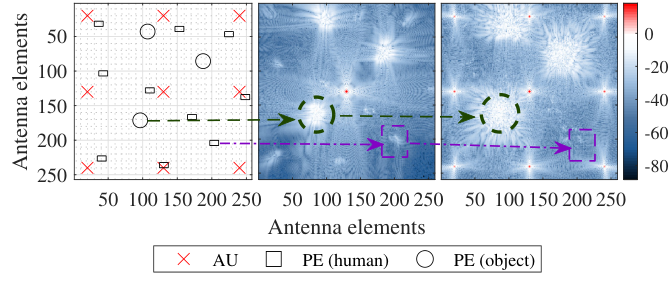
To illustrate, we consider the scenario described in Appendix A, where we have AUs and PEs with of them being cylindrical metallic objects and humans. Fig. 2 contains (a) the ground truth RM, where the AUs are represented by red crosses, while the PEs by the geometrical forms – metallic objects by the circles and the humans by the rectangles – (b) the RM of a single AU; and (c) the RM of superposed signals of the AUs. The MF filter used was the same as in [4], with computed as in (4). Fig. 2(b) exposes the effect of the distortion around the LoS components with power as high as the rays reflected by PEs. Fig. 2(c) shows the behavior when the signals are superposed. Specifically, we see how the metallic objects are highlighted while the humans get occluded, making it more difficult to correctly detect the latter.
IV OnRMap
Here we present OnRMap, an online RMap approach based on classical signal processing theory, which removes the need for offline scanning phases from [4, 5]. We detail the four stages that comprise OnRMap until we sense and locate the AUs and PEs, with an emphasis on the PEs, which are the most challenging to be detected.
IV-A OnRMap: An Overview
OnRMap consists of four steps, illustrated in Fig. 3.
Step 0. Signal Acquisition and Primary RM. In this initial step, we obtain the contributions from the AUs to the primary RM by filtering the signals with the MF given in Eq. (5). Different from [4] and based on the discussion made in Section III, we empirically chose the weight vector using a two dimensional (2-D) Taylor window [12]. This selection was motivated by the empirical reduction of filtering distortion and numerical improvement in the ratio between the NLoS components. The output of this step is the matrix containing the primary RMs stacked in columns, i.e., , where here denotes element-wise absolute value.
Step 1. Estimation of the LoS and NLoS Components. Through this step, the primary RM in is the input to the robust principal component analysis (RPCA) algorithm [13], which outputs the matrices and corresponding to the estimations of the LoS and NLoS components of , respectively. We employ this method based on the observation that the NLoS components have similarities among themselves, e.g., the range of the power gain and location. In contrast, LoS components are a few data points with high power gains that are normally far apart. Hence, we can interpret the NLoS components to be low-rank components of , whereas the LoSelements are sparse. Thus, RPCA becomes useful, since it is a low-complexity method for estimating the low-rank components of a matrix. Based on the special focus on sensing and locating the PEs, this block outputs the low-rank estimation, .
Step 2. Separation of the NLoS Components. This step translates the NLoS estimation from the previous step into data points for the inference step. To do so, we input in k-means clustering [14], which separates the data in two clusters that represent foreground ( high power) and background (low power) classes differentiate by their power level. The foreground forms shapes in 2-D space and their perimeters are estimated with the Moore-Neighbor boundaries estimation algorithm [15]. The points that enclose the perimeters are stored in subsets that compound the set and the total power levels each shape comprises in are stored in the set , constituting the output of this step.
Step 3. Sensing and Localization Inference. In this final block, we use the data in and to infer whether each subset in is a type of PE or just noise. If it is a PE, we can further identify which type of object it is, e.g., a human or a metallic object, and their positions are also inferred. To do so, we employ Density-based spatial clustering of applications with noise (DBSCAN) clustering method [16] to cluster the data in based on the distance between samples. It is also assigned to each cluster its total power by looking at the set . The classification of each cluster on which type of PE(metallic object or human) follows a decision rule based on the power each cluster has, that is, lower and upper bounds are defined, and the clusters that fit in between are considered humans, those above are considered as objects, while the rest is noise.
IV-B OnRMap: Detailed Description
Below, we give further details on the other steps apart from Step 0, which was already detailed in (5).
IV-B1 Estimation of the LoS and NLoS Components
RPCA solves the following optimization problem [13]:
| (7) |
where is the observation matrix, and are estimations of the low-rank and sparse components of , respectively, and are the nuclear and norm of a matrix, respectively, and is a scalar. In our case, from Step 0 we have the matrix , which is obtained by stacking and normalizing the , . Then, we decompose it as:
| (8) |
Define and as estimations of and , respectively. Then, substituting in Eq. (IV-B1), we have
| (9) |
placing the separation of LoS and NLoS components as equivalent to the optimization problem in (IV-B1). The output of the algorithm is summed row-wise and reshaped to ; the same for the LoS-related matrix.
To illustrate how well RPCA performs, Fig. 4 shows the recovered low-rank (left) and sparse matrix (right). As can be seen, RPCAcan estimate satisfactorily the NLoS(left) and LoS(right) components. On the other hand, we can point out two disadvantages of this technique. First, although there is a reference value for , it may have to be tuned according to the scenario. Second, the problem of estimating low-rank and sparse components of matrices is NP-hard. RPCA solves a convex relaxed problem, incurring some information loss. However, most of the time, this method estimates satisfactory the components within less than twenty iterations. Despite that, for some realizations, part of the PEs was outputted in the sparse (LoS) component.

IV-B2 Separation of the NLoS Components
First, let’s define the binary k-means clustering operation as . Then, we perform entry-wise , with being the matrix with the class of each data point in . In particular, we name class 0 as background containing points with null to very low power and class 1 as foreground containing components above a certain power threshold. We illustrate the output of the k-means on the left side of Fig. 5. Note the creation of certain regions that can be interpreted as geometrical shapes. Visually inspecting and comparing the shapes with the ground truth, Fig. 2(a), we can infer that components that represent the metallic objects are more likely to be clustered in a larger and denser area, while the humans’ ones are smaller and sparser.
Based on the observation made above, we employ the Moore-Neighbor boundaries estimation algorithm [15] to leverage these regions to detect the PEs. The boundary estimation algorithm works in the following way. First, a random point with value ’1’ (foreground) in is picked up, defined as a central point, and its eight-point neighborhood values are checked. Then, the neighbors that have value ’1’ to this central point are considered to be in the same region as the central points. The algorithm starts by further searching considering the neighborhood of newfound points. Finally, a shape is defined when there are no other points left with the value ’1’ around the perimeter, where the outermost points are retrieved as a perimeter. Both perimeter and internal points are defined by tuples representing the column and row in which they are allocated in the matrix. The perimeter points are assigned to a subset and all the points that define a shape in , where indexes a shape. Then, we associate a value to each region depicting the total power level within that region, which is calculated as:
| (10) |
The values ’s are further stored in the set . The boundaries for this scenario can be seen on the right side of Fig. 5.

IV-B3 Sensing and Localization Inference
This block receives the sets and and does the inference process. First, the data is clustered with DBSCAN [16]. This method randomly chooses a core point by observing the data in and maps the neighborhood subject to and constraint parameters, representing the minimum number of points in a cluster and the search radius, respectively. Starting from the core point, the algorithm calculates the distances to all points in the data and assigns as a cluster those that satisfy the parameter constraints. The process is repeated until all the data have been clustered. Points that are sparsely distributed and thus cannot be assigned to a cluster, are considered noise. The indexes of the shapes that compound each cluster are assigned to the -th cluster that maps both and sets.
We perform a test of the described algorithm on the illustrative scenario in Appendix A with and . The algorithm output 63 identified clusters, which is much higher than the true number of PEs in the environment. To overcome excessive number of clusters, we exploit the metallic objects’ lower reflection loss than the humans, , so we can infer that clusters with high power are objects, while clusters with low powers are noise or background distortion; consequently, clusters in the middle represent human positions. Thus, the -th cluster is considered to be of a human class if it satisfies the following rule over :
| (11) |
where and are the minimum and maximum threshold parameters, respectively. If the cluster passes the threshold rule, then the cluster centroid is stored in a new set of detected humans .
To evaluate how reasonable the inference is, let be the vector containing the differences between the inferred and the ground truth localization of the humans, giving the localization accuracy per human. Its -th entry is calculated as:
| (12) |
where denotes the -th element of and is the set of ground-truth humans with the -th element denoted as and whose cardinality is . Furthermore, is the Euclidean norm. We adopt as m the distance threshold for detection via experimentation. The value of accuracy can be null in case the distance is higher than the one defined by the threshold; in this case, we assume . We define the localization accuracy, , and the detection rate, , as:
| (13) |
where is the indicator function.
By empirically setting set and , Fig. 6 shows how the data were clustered for the illustrative example of Appendix A. Overall, it was identified 67 clusters, where three have very high energy, corresponding to the metallic objects, ten with low to medium energy, corresponding to humans, and the rest with shallow energy, considered noise. To visually assess the quality of the results, we re-plot on the right side of the figure the ground truth points together with the inferred points. The algorithm was capable of inferring the human’s positions with localization accuracy from m (best case) to m (worst case) and the average of m in this single realization.
V Numerical results
We now evaluate the effectiveness of OnRMap and compare it with the previous works [4, 5]. For a better evaluation, we consider a more complex indoor scenario as provided by Feko by Altair Engineering ray tracing, as used in [4]. Different from the system model and toy example presented, this scenario includes more reflections from the PEs and reflections from the ground and walls. Despite that, the other parameters are the same as in Appendix A with metallic objects and humans. Throughout this section, we focus on showing results for human detection since the detection of AUs and metallic objects is less challenging.
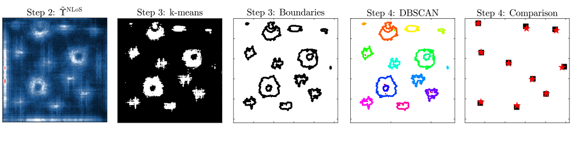
We start by illustrating a step-by-step realization of OnRMap in Fig. 7 with AUs. From the figure, we can note that OnRMap can perform well even in this more unfavorable scenario, given the increase in multipath components. In Fig. 8, we better evaluate the performance of OnRMap by considering 1000 Monte Carlo simulations (MCSs). Fig. 8a shows the average localization accuracy and the average detection rate of the humans when considering different numbers of AUs. We compare these results with the ones presented in [4]. The trade-off in the comparison is that we can achieve higher localization accuracy for all numbers of AU configurations () at the cost of lower detection rates on average. It is possible to point out two causes of the lower detection performance compared to [4]. First, some information of the signals is filtered after RPCA and does not enter in the inference process, as opposed to [4] that treats the signals from all AUs. Second, when the boundaries among PEs from different classes are too close, DBSCAN classify them as one cluster and the decision rule considers both as just one type of PE. These are considered the costs of the proposed online method in view of the offline approach. The lack of a priori information to compensate static PEs as in [4], compromises the to some extent. However, we argue that the high applicability and the significant improvement in the overall justify the novelty of this work.
To better understand the impact of the number of AUs in the detection rate, Fig. 8b shows the complementary cumulative distribution function (CCDF) of the detection in terms of the number of correctly detected humans for different numbers of AUs . Note that the effect of increasing is to lower the variance on how many humans we can detect. However, the opposite occurs at the points of nine to ten correctly detected humans, highlighted in Fig. 8b. For , the probability of a perfect detection (ten humans) is 0.4 %, and when it achieves 3.2 %. A reason for this is that higher implies more signals reflecting on PEs that can be possibly distributed next to the center of the room, while the PEs next to the walls are less exposed, and those reflections start to be interpreted as background (distortion/noise) by the method.
VI Conclusions
In this paper, we proposed OnRMap, an online method for sensing and localization in indoor environments equipped with LIS systems. The greatest advantages of OnRMap are due to the fact that it is based on signal processing techniques, making it an online method, that is, it does not rely on offline scanning phases. This makes the method more robust for applications where the environment is constantly changing. However, the online feature comes with the cost of an average lower detection rate. But even so, OnRMap turns out to have a fairly good location accuracy. Future works may improve the design of OnRMap to cover the observed weakness and better study its performance.
Appendix A An Illustrative Indoor Scenario
The parameters of the simulation scenario are summarized in Table I. Note that we consider a scenario with two types of PEs: i) cylindrical metal objects with polished surfaces dB and humans dB, totaling PEs.
| Parameter | Value | Parameter | Value |
|---|---|---|---|
| Environment | Channel & System | ||
| # PEs | = 3 | Trans. power | [dBm] |
| = 10 | Noise power | [dBm] | |
| Room dim. | (y) = 10.36 [m] | LoS PL | |
| (x) = 10.36 [m] | NLoS ref. loss | dB | |
| (z) = 8 [m] | dB | ||
| Obj. dim | rad. = 0.43 [m] | Carr. freq. | [GHz] |
| (z) = 2 [m] | Carr. wavel. | [m] | |
| Hum. dim. | (y) = 0.3 [m] | Active users | |
| (x) = 0.5 [m] | # AUs | ||
| (z) = 1.7 [m] | AUs height | [m] | |
| LIS pos. | [m] | ||
| LIS elem. | |||
References
- [1] S. Hu, F. Rusek, and O. Edfors, “Beyond massive MIMO: The potential of data transmission with large intelligent surfaces,” IEEE Trans. Signal Process, vol. 66, no. 10, pp. 2746–2758, 2018.
- [2] D. Dardari, “Communicating with large intelligent surfaces: Fundamental limits and models,” IEEE J. Sel. Areas Commun., vol. 38, no. 11, pp. 2526–2537, 2020.
- [3] C. J. Vaca-Rubio, P. Ramirez-Espinosa, K. Kansanen, Z.-H. Tan, E. De Carvalho, and P. Popovski, “Assessing wireless sensing potential with large intelligent surfaces,” IEEE Open Journal of the Communications Society, vol. 2, pp. 934–947, 2021.
- [4] C. J. Vaca-Rubio, P. Ramirez-Espinosa, K. Kansanen, Z.-H. Tan, and E. de Carvalho, “Radio sensing with large intelligent surface for 6g,” 2021. [Online]. Available: https://arxiv.org/abs/2111.02783
- [5] C. J. Vaca-Rubio, R. Pereira, X. Mestre, D. Gregoratti, Z.-H. Tan, E. De Carvalho, and P. Popovski, “Floor map reconstruction through radio sensing and learning by a large intelligent surface,” in 2022 IEEE 32nd International Workshop on Machine Learning for Signal Processing (MLSP). IEEE, 2022, pp. 1–6.
- [6] X. Tong, Z. Zhang, Y. Zhang, Z. Yang, C. Huang, K.-K. Wong, and M. Debbah, “Environment sensing considering the occlusion effect: A multi-view approach,” IEEE Transactions on Signal Processing, vol. 70, pp. 3598–3615, 2022.
- [7] X. Tong, Z. Zhang, J. Wang, C. Huang, and M. Debbah, “Joint multi-user communication and sensing exploiting both signal and environment sparsity,” IEEE Journal of Selected Topics in Signal Processing, vol. 15, no. 6, pp. 1409–1422, 2021.
- [8] J. Wilson and N. Patwari, “Radio tomographic imaging with wireless networks,” IEEE Trans. Mobile Comput., vol. 9, no. 5, pp. 621–632, 2010.
- [9] M. Zhao, T. Li, M. Abu Alsheikh, Y. Tian, H. Zhao, A. Torralba, and D. Katabi, “Through-wall human pose estimation using radio signals,” in Proc. IEEE Conf. Comput. Vis. Pattern Recognit., 2018, pp. 7356–7365.
- [10] A. Saleh and R. Valenzuela, “A statistical model for indoor multipath propagation,” IEEE Journal on Selected Areas in Communications, vol. 5, no. 2, pp. 128–137, 1987.
- [11] A. Goldsmith, Wireless Communications. Cambridge University Press, 2005.
- [12] E. Brookner, Practical Phased Array Antenna Systems. Artech House, 1991.
- [13] E. J. Candès, X. Li, Y. Ma, and J. Wright, “Robust principal component analysis?” J. ACM, vol. 58, no. 3, jun 2011. [Online]. Available: https://doi.org/10.1145/1970392.1970395
- [14] D. Arthur and S. Vassilvitskii, “k-means++: The advantages of careful seeding,” in SODA ’07: Proceedings of the eighteenth annual ACM-SIAM symposium on Discrete algorithms. Philadelphia, PA, USA: Society for Industrial and Applied Mathematics, 2007, pp. 1027–1035.
- [15] R. Gonzalez, R. Woods, and S. Eddins, Digital Image Processing Using MATLAB. Pearson Prentice Hall, 2004.
- [16] M. Ester, H.-P. Kriegel, J. Sander, and X. Xu, “A density-based algorithm for discovering clusters in large spatial databases with noise,” in Proceedings of the Second International Conference on Knowledge Discovery and Data Mining, ser. KDD’96. AAAI Press, 1996, p. 226–231.