Spectral comparison of compound cocycles generated by delay equations in Hilbert spaces

Abstract

We study linear cocycles generated by nonautonomous delay equations in a suitable Hilbert space and their extensions, called compound cocycles, to exterior powers. Using a recent version of the frequency theorem, we develop analytical techniques for comparing spectral properties, such as uniform exponential dichotomies, between such cocycles and semigroups generated by stationary equations. These methods are based on properties related to regularity and structure in PDEs associated with delay equations. In particular, the developed machinery leads to effective robust criteria that guarantee the absence of closed invariant contours on global attractors arising in nonlinear problems and are expected to ensure global stability.

Contents

1 Introduction

1.1 Historical perspective: Lyapunov dimension and effective dimension estimates for delay equations

In the study of dissipative dynamical systems, structure of attractors takes the spotlight. A classical question of this kind, especially interesting in infinite-dimensions, is related to obtaining effective dimension estimates for global attractors. Although the initial motivation for the problem was concerned with finite-dimensional reduction based on embedding theorems for sets with finite Hausdorff or fractal dimensions (see [44, 51, 52]), the volume contraction approach revealed a more relevant dimension-like characteristic called the Lyapunov dimension¹¹ 1 More precisely, such a quantity is called the uniform (or global) Lyapunov dimension to distinguish it from the Lyapunov dimension over an ergodic measure. This distinction is not necessary for the present work where only the uniform quantity is considered.. Roughly speaking, it is determined by the dimension threshold such that infinitesimal volumes of higher dimensions admit uniform exponential decay. It is well known that such a quantity always bounds from above the fractal dimension of the invariant set (or its fibers in the case of cocycles), see [17, 28, 48]. However, unlike purely geometric dimensions, it is more robust (namely, upper semicontinuous) and admits computation on the infinitesimal level with the aid of adapted metrics, see [25, 1]. Even if an exact value of the Lyapunov dimension is known, it often reflects not any geometric dimensions of the global attractor, but rather possible expansions of such dimensions under perturbations of the system; see [50] for a nice example. Armed with upper estimates for the Lyapunov dimension, we have a generalized Bendixson criterion which indicates the absence of certain invariant structures on the attractor, see [46, 34]. In particular, conditions which guarantee a uniform decay of two-dimensional volumes provide criteria for the global stability by utilizing the robustness and variants of Pugh’s Closing Lemma, see [3, 33, 46]. We refer to the surveys [51, 52] for more discussions on the theory of attractors and finite-dimensional reduction and to our papers [1, 3, 4] for more discussions concerned with effective dimension estimates and the problem of global stability by means of delay equations.

There is a variant of the Lyapunov dimension (generally producing slightly larger values) based on the Kaplan–Yorke formula involving uniform Lyapunov exponents [1]. A classical result²² 2 This result holds in a much wider (than it is stated in [24]) generality covering infinite-dimensional noninvertible systems in virtue of the variational principle and the Margulis–Ruelle inequality, see [49, 14]. of Katok [24] bounds the topological entropy from above via the sum of positive uniform Lyapunov exponents³³ 3 Among control theorists, this sum is known as the restoration entropy, see [25].. Along with the above, this illustrates relations between dimension, entropy, and volume in the context of uniform characteristics.

Here we follow the volume contraction approach which is concerned with obtaining upper estimates for the growth exponents of infinitesimal volumes over an invariant set $\mathcal{Q}$ . More rigorously, we are interested in upper estimates for the largest uniform Lyapunov exponent $\lambda_{1}(\Xi)$ of the derivative cocycle $\Xi$ over the invariant set and its extensions $\Xi_{m}$ (called compound cocycles) to exterior powers $\mathbb{H}^{\wedge m}$ of a certain Hilbert space $\mathbb{H}$ . On the abstract level, it will be sufficient to work with linear cocycles over a semiflow on a complete metric space (possibly noncompact).

In terms of the general computational scheme presented in [1], to estimate $\lambda_{1}(\Xi_{m})$ from above, one should choose a suitable (adapted) metric given by a family of inner products in $\mathbb{H}^{\wedge m}$ depending on $q\in\mathcal{Q}$ and apply certain maximization procedures to the infinitesimal quantities arising from differentiation of the cocycle trajectories in the metric. These quantities are involved into the Growth Formula, which reduces to the Liouville trace formula if the metric is associated with a metric in $\mathbb{H}$ . In the latter case, the variational problem can often be reduced to the computation of eigenvalues of self-adjoint operators. In infinite dimensions, such computations are usually done in standard metrics (see [48, 17, 51]), although it may happen that standard metrics may not be relevant, as in the case of delay equations [4, 1, 7] or hyperbolic equations [51, 50].

In finite dimensions, there is an approach known as the Leonov method [32, 29, 1]. On the geometric level, it corresponds to variations of a constant metric in its conformal class via Lyapunov-like functions. This method often allows to improve estimates or even provide exact computations of the Lyapunov dimension, as in the case of Lorenz, Lorenz-like, and Hénon systems; see [28, 27, 31, 30].

It is also worth mentioning the approach of Smith [46] for ODEs based on quadratic functionals that allows to bound from below all the singular values of the derivative cocycle. In applications, his method goes in the spirit of the perturbative approach that we follow here. For infinite-dimensional systems, it can be developed via inertial manifolds; see [7, 8]. However, this reveals its impracticality and artificiality for the problem.

In the case of delay equations, the problem of obtaining effective dimension estimates remained without significant progress for a long time, see [1] for a more detailed discussion. This is reflected in some past [21] and relatively recent monographs [18, 16], which essentially expand the ideas from the pioneering paper [41] by exploiting the compactness of the derivative cocycle and hence making only qualitative conclusions on the finiteness of dimensions. In [1], we resolved the problem by explicitly constructing constant adapted metrics for a fairy general class of delay equations in $\mathbb{R}^{n}$ with discrete delays. For global attractors arising in the Mackey–Glass equations [38] and the periodically forced Suarez–Schopf delayed oscillator [6, 47], numerical experiments suggest that the obtained estimates are asymptotically sharp as the delay tends to infinity. In [4], the approach is illustrated by means of the Nicholson blowflies model. However, obtaining more accurate estimates for specific parameters remains a challenging task.

All the above results concern the use of metrics on exterior powers, which are associated with a metric on $\mathbb{H}$ . For computation, this allows to avoid direct examinations of compound cocycles and their infinitesimal generators and remain only on the level of linearized equations. However, as it is argued in [1] by means of Lyapunov-like metrics, for theory⁴⁴ 4 For finite-dimensional invertible systems, the result of [25], based on what we call Shannon-like metrics (see [1]), shows that theoretically it is sufficient to work only with associated metrics. However, we note that Lyapunov-like metrics (used in [1]) also arise in applications of the frequency theorem to study compound cocycles, which is the topic of the present paper. and practice, it may be natural to use adapted metrics defined on exterior powers. In the present work we follow this line, see Section 1.2.

Besides [1], a rare exception in the field, which partly motivated the present work, is the work of Mallet-Paret and Nussbaum [39], where compound cocycles in Banach spaces generated by certain scalar nonautonomous delay equations are studied. Such equations particularly arise after linearization of scalar delay equations with monotone feedback, which are known to satisfy the Poincaré–Bendixson trichotomy [40]. In [39], it is shown that the $m$ -fold compound cocycle preserves a convex reproducing normal cone in the $m$ -fold exterior power for either odd or even (the most interesting case) $m$ depending on the feedback sign. Based on this, the authors developed the Floquet theory for periodic equations using arguments in the spirit of the Krein–Rutman theorem. In particular, it is stated a comparison principle that allows to compare Floquet multipliers for periodic (in particular, stationary) equations. This principle can be developed to obtain effective dimension estimates, see [7]. However, scalar equations (not to mention systems of equations) that exhibit chaotic behavior are beyond the scope of this approach.

In what follows, we present another approach to the problem of effective dimension estimates for delay equations, based on direct examinations of compound cocycles and their generators.

1.2 Contribution of the present work

In this paper, we study a sufficiently general class of linear nonautonomous delay equations in $\mathbb{R}^{n}$ as it is described in (6.1). As in our adjacent work [1], we address the problem of obtaining conditions for the exponential stability of compound cocycles corresponding to such equations. We are aimed to express such conditions in terms of frequency inequalities arising from a comparison between compound cocycles $\Xi_{m}$ and certain $C_{0}$ -semigroups $G^{\wedge m}$ with the aid of the frequency theorem developed in our work [5]. In fact, we will obtain conditions for the existence of gaps in the Sacker–Sell spectrum [45], i.e., uniform exponential dichotomies, and even more, see Theorem 6.2 and the remarks below. As will be shown, following this program reveals novel functional-analytic properties of delay equations concerned with harmonic analysis, see below.

In our adjacent work [3], we developed approximation schemes to verify such frequency inequalities and applied them to derive effective criteria for the absence of closed invariant contours on global attractors for scalar equations. Our experiments indicate improvements of the known rare results in the field. For $m=2$ and equations with single delays, it was observed that the associated transfer operators can be expressed as integral operators with explicitly given $L_{2}$ -summable kernels. In [2], we exploited the optimization of Schur test functions to check inequalities that reduce to estimating norms of transfer operators. Similar considerations are applicable for systems of equations and will be expounded in a future paper. A brief discussion of these results is given in Section 7.

Let us expose main ideas and methods of our work. For precise preliminary definitions and notations, we refer to Sections 2 and 3.

First, we treat delay equations in the Hilbert space $\mathbb{H}$ defined by (4.1), based on our work [7]. This contrasts with [39] and most other works, where delay equations are posed in the space of continuous functions. Such a treatment is essential for our functional-analytical study of delay equations as PDEs with nonhomogeneous boundary conditions, see [35]. On the other hand, thanks to the smoothing properties of dynamics, the final conclusions concerning asymptotic behavior in the norm of $\mathbb{H}$ are also fulfilled in the usual supremum norm.

Basically, we treat the $m$ -fold compound cocycle $\Xi_{m}$ on the $m$ -fold exterior power $\mathbb{H}^{\wedge m}$ of $\mathbb{H}$ as a nonautonomous perturbation of a stationary cocycle which is a $C_{0}$ -semigroup $G^{\wedge m}$ . In terms of (6.1), the stationary linear part is distinguished, and to it corresponds an operator $A$ , which generates a $C_{0}$ -semigroup $G$ in $\mathbb{H}$ . Then $G^{\wedge m}$ is given by the (multiplicative) extension of $G$ onto $\mathbb{H}^{\wedge m}$ . On the infinitesimal level, $G^{\wedge m}$ is generated by an operator $A^{[\wedge m]}$ , called the (antisymmetric) additive compound of $A$ . In Theorem 6.1, the infinitesimal generator of $\Xi_{m}$ is described as a nonautonomous boundary perturbation of $A^{[\wedge m]}$ . It is essential to use the Hilbert space setting to make sense of the boundary perturbation.

After that, we study the problem of providing conditions for preserving certain dichotomy properties of $G^{\wedge m}$ for all perturbations in a given class (for example, with a prescribed Lipschitz constant). Here, the perturbation class is described through an indefinite quadratic form, for which we consider the associated infinite-horizon quadratic regulator problem posed for a proper linear control system. The latter problem is resolved using the frequency theorem developed in our paper [5]. It provides frequency conditions for the existence of a quadratic Lyapunov functional for $\Xi_{m}$ , which can be used to obtain the desired dichotomy properties.

Note that the described approach can potentially be applied to a range of problems enjoying a kind of asymptotic compactness such as semilinear parabolic equations, damped hyperbolic equations, neutral delay equations, or parabolic equations with nonlinear boundary conditions. However, apart from our studies, we are not aware of any works devoted to this, even in the case of ODEs.

As to delay equations, they represent analytically nontrivial examples of such applications. Here, some problems arise mainly due to the unbounded nature of perturbations on the infinitesimal level. This demands distinguishing between regularity and structure in the associated linear inhomogeneous problems⁵⁵ 5 Roughly speaking, regularity is related to various spectral bounds or estimates for resolvents in intermediate spaces, and structure is related to tempo-spatial properties of solutions. For example, in the case of semilinear parabolic equations in bounded domains, tempo-spatial properties, known as parabolic smoothing, come from the resolvent and spectrum bounds (see [9, 18]). Thus, it is quite fair to attribute these properties to regularity (not mentioning their “structurality”), as is always done. However, for delay equations, the issue of distinguishing becomes acute.. In our work [5], we explored some related features that allow to resolve these obstacles in the case $m=1$ . In this paper, the main part is devoted to the generalization of these properties for general $m$ . They do not follow from the case $m=1$ , and therefore it is necessary to develop an appropriate theory.

On the side of structure, we establish what was called in [5] a structural Cauchy formula, see Theorem 5.1. This is a certain decomposition of mild solutions to linear inhomogeneous problems associated with $A^{[\wedge m]}$ (more generally, with $A^{[\otimes m]}$ ), which differs from the usual Cauchy formula, but reveals a certain structure of solutions. More precisely, according to the formula, each component of a solution is uniquely decomposed into the sum of what we call adorned and twisted functions. In its turn, such a sum is called by us an agalmanated function, and the corresponding functional spaces are introduced in Appendix B. To prove and understand Theorem 5.1, preparatory results on diagonal translation semigroups and diagonal Sobolev spaces from Appendix A are also required.

We use the structural Cauchy formula to make sense of integral functionals arising in the quadratic regulator problem. Here, what we call pointwise measurement operators naturally arise, and they are studied in Appendix B. Such operators are defined by pointwise application of a certain unbounded operator⁶⁶ 6 For example, a $\delta$ -functional in some $L_{2}$ -space. to a function of time. They are naturally defined on what we call embracing spaces, into which the aforementioned classes of functions can be naturally embedded. Note that for the case of adorned functions and $m=1$ , the well-posedness of pointwise measurement operators reflects convolution theorems for measures, see [22]. However, we cannot find a general result that covers our situation for $m>1$ , let alone the other classes of functions. Another key property of embracing spaces is that the Fourier transform in $L_{2}$ provides an automorphism of the embracing space (over $\mathbb{R}$ ) and commutes with pointwise measurement operators. This constitutes Theorem B.3, which is important for deriving frequency inequalities.

On the side of regularity, we establish certain uniform bounds for the resolvent in intermediate spaces, see Theorem 4.4. This constitutes the second main ingredient for resolving the quadratic regulator problem and establishing our final Theorem 6.2.

For applications of the frequency theorem to other problems also involving certain dichotomies, we refer to our works on inertial manifolds [5, 8, 9] and almost periodic cocycles [10, 11, 12].

1.3 Structure of the present work

Now we will describe the structure of our work, indicating the key points.

To the best of our knowledge, the widespread interest in the theory of multiplicative and additive compounds began with the work of Muldowney on ODEs [43]. Recently, Muldowney and Wang [42] presented an algebraic theory of additive and multiplicative compound operators in general linear spaces. For us, it is important the spectral theory of such operators in Hilbert spaces, which we cannot find in the existing literature. For this, we develop an appropriate theory in Sections 2 and 3.

In Section 4, we study additive compounds $A^{[\otimes m]}$ and $A^{[\wedge m]}$ of delay operators $A$ . This includes describing the abstract $m$ -fold tensor product $\mathbb{H}^{\otimes m}$ of $\mathbb{H}$ in terms of a certain $L_{2}$ -space, see Theorem 4.1; the action of $A^{[\otimes m]}$ , see Theorem 4.2; the domain $\mathcal{D}(A^{[\otimes m]})$ , see Theorem 4.3; and deriving bounds for the resolvent in intermediate spaces, see Theorem 4.4.

In Section 5, we establish a structural Cauchy formula for linear inhomogeneous problems associated with $A^{[\otimes m]}$ (in particular, $A^{[\wedge m]}$ ), see Theorems 5.1 and 5.2.

In Section 6, linear cocycles generated by a class of delay equations are studied. In Section 6.1, infinitesimal generators of the corresponding multiplicative compound cocycles in $\mathbb{H}^{\otimes m}$ (resp. $\mathbb{H}^{\wedge m}$ ) are described as nonautonomous boundary perturbations of $A^{[\otimes m]}$ (resp. $A^{[\wedge m]}$ ), see Theorem 6.1. In Section 6.2, related linear inhomogeneous problems with quadratic constraints are formulated. In Section 6.3, the associated integral quadratic functionals are interpreted and their relation with the Fourier transform is established, see Lemma 6.2. In Section 6.4, frequency inequalities for the preservation of certain dichotomy properties under the perturbations are derived, see Theorem 6.2.

In Section 7, we discuss analytical-numerical methods to verify frequency inequalities for concrete problems. In particular, we briefly explain ideas and experimental results from our adjacent work [3].

In Appendix A, the theory of diagonal translation semigroups and diagonal Sobolev spaces is developed.

In Appendix B, pointwise measurement operators on embracing spaces are studied. In particular, the spaces of adorned, twisted, and agalmanated functions are introduced.

Some general notations

Throughout the paper, $m$ , $n$ , $k$ , $l$ , and $j$ denote natural numbers. Usually, $m$ and $n$ are fixed; $j\in\{1,\ldots,m\}$ ; $k$ is used to denote the size of multi-indices such as $j_{1}\ldots j_{k}$ with $1\leq j_{1}<\cdots<j_{k}\leq m$ ; $l$ is used for indexing sequences. Real numbers are denoted by $t$ , $s$ or $\theta$ , where, usually, $t,s\geq 0$ and $\theta\in[-\tau,0]$ for some $\tau>0$ being a fixed value (delay).

For distinct integers $j_{1},\ldots,j_{k}$ and $j$ , we define $J(j)=J(j;j_{1},\ldots,j_{k})$ as the integer $J\in\{1,\ldots,k+1\}$ such that $j$ is the $J$ th element of the set $\{j,j_{1},\ldots,j_{k}\}$ , arranged by increasing.

We often use the excluded index notation to denote multi-indices. For example, in the context of given $j_{1}\ldots j_{k}$ and $i\in\{j_{1},\ldots,j_{k}\}$ , we denote by $j_{1}\ldots\hat{i}\ldots j_{k}$ the multi-index of size $k-1$ obtained from $j_{1}\ldots j_{k}$ by removing $i$ . For brevity, we also write $\hat{i}$ instead of $j_{1}\ldots\hat{i}\ldots j_{k}$ , if it is clear from the context what multi-index is meant. A similar notation is used for the exclusion of several indices.

For the compactness of formulas, it is often convenient to use $\bar{s}$ or $\bar{\theta}$ to denote vectors of real numbers. For example, $\bar{s}=(s_{1},\ldots,s_{m})\in\mathbb{R}^{m}$ or $\bar{\theta}=(\theta_{1},\ldots,\theta_{m})\in[-\tau,0]^{m}$ . Sometimes the excluded index notation for these vectors is also used in different ways. For example, by $\bar{s}_{\hat{j}}$ we denote the $(m-1)$ -vector appearing after eliminating the $j$ th component from $\bar{s}$ . Moreover, the same vector is denoted by $(s_{1},\ldots,\hat{s}_{j},\ldots,s_{m})$ .

Given a real number $t\in\mathbb{R}$ , we use $\underline{t}$ to denote the vector with identical components, all of which equal to $t$ . Its dimension should be understood from the context. For example, if $\bar{s}\in\mathbb{R}^{m}$ , then in the sum $\bar{s}+\underline{t}$ we have $\underline{t}\in\mathbb{R}^{m}$ .

We use $\mu^{k}_{L}$ to denote the $k$ -dimensional Lebesgue measure. This notation is used mainly in cases where it should be emphasized that we are dealing with $\mu^{k}_{L}$ -almost all elements of a certain $k$ -dimensional subset.

We use $\|\cdot\|_{\mathbb{E}}$ to denote the norm in a Banach space $\mathbb{E}$ . In the case of a Hilbert space $\mathbb{H}$ , we often (mainly in the context of $\mathbb{H}$ -valued functions) use $|\cdot|_{\mathbb{H}}$ to denote the norm. Moreover, the inner product in $\mathbb{H}$ is denoted by $\langle\cdot,\cdot\rangle_{\mathbb{H}}$ .

Given Banach spaces $\mathbb{E}$ and $\mathbb{F}$ , we use $\mathcal{L}(\mathbb{E};\mathbb{F})$ to denote the space of bounded linear operators between them. If $\mathbb{E}=\mathbb{F}$ , we write just $\mathcal{L}(\mathbb{E})$ . For the corresponding operator norm, we use the notation $\|\cdot\|_{\mathcal{L}(\mathbb{E};\mathbb{F})}$ or simply $\|\cdot\|$ , if the spaces are understood from the context. For the identity operator in $\mathbb{E}$ , we use the notation $\operatorname{Id}_{\mathbb{E}}$ . Often the same operator is denoted by $I$ , if the space is understood from the context.

2 Multiplicative compounds on tensor products of Hilbert spaces

In this section, we briefly recall some facts about tensor products of Hilbert spaces.

Let $\mathbb{H}_{1}$ and $\mathbb{H}_{2}$ be real or complex Hilbert spaces with inner products⁷⁷ 7 In the case of complex spaces, we use the convention that sesquilinear (Hermitian) forms are linear in the first argument and conjugate-linear in the second. $\langle\cdot,\cdot\rangle_{\mathbb{H}_{1}}$ and $\langle\cdot,\cdot\rangle_{\mathbb{H}_{2}}$ . Let $\mathbb{H}_{1}\odot\mathbb{H}_{2}$ denote the algebraic tensor product of these spaces. Recall that it is spanned by the elements $v_{1}\otimes v_{2}$ , where $v_{1}\in\mathbb{H}_{1}$ and $v_{2}\in\mathbb{H}_{2}$ , called decomposable tensors. As an operation, $v_{1}\otimes v_{2}$ is bilinear and called the tensor product of $v_{1}$ and $v_{2}$ .

There is a natural inner product on $\mathbb{H}_{1}\odot\mathbb{H}_{2}$ , which is defined for decomposable tensors $v_{1}\otimes v_{2}$ and $w_{1}\otimes w_{2}$ by

\langle v_{1}\otimes v_{2},w_{1}\otimes w_{2}\rangle_{\mathbb{H}_{1}\otimes\mathbb{H}_{2}}\coloneq\langle v_{1},w_{1}\rangle_{\mathbb{H}_{1}}\langle v_{2},w_{2}\rangle_{\mathbb{H}_{2}}.

(2.1)

Using standard arguments appealing to the universal property of algebraic tensor products, it can be shown that (2.1) correctly extends to an inner product on $\mathbb{H}_{1}\odot\mathbb{H}_{2}$ . Then the tensor product $\mathbb{H}_{1}\otimes\mathbb{H}_{2}$ of Hilbert spaces $\mathbb{H}_{1}$ and $\mathbb{H}_{2}$ is defined by the completion of $\mathbb{H}_{1}\odot\mathbb{H}_{2}$ by the inner product from (2.1). Sometimes it may be convenient to emphasize the field, i.e., $\mathbb{R}$ or $\mathbb{C}$ , over which the tensor product is taken. For this, we use the notations $\mathbb{H}_{1}\otimes_{\mathbb{R}}\mathbb{H}_{2}$ or $\mathbb{H}_{1}\otimes_{\mathbb{C}}\mathbb{H}_{2}$ , respectively.

Let $\mathbb{W}_{1}$ and $\mathbb{W}_{2}$ be another Hilbert spaces over the same field as $\mathbb{H}_{1}$ and $\mathbb{H}_{2}$ . Given bounded linear operators $L_{1}\colon\mathbb{H}_{1}\to\mathbb{W}_{1}$ and $L_{2}\colon\mathbb{H}_{2}\to\mathbb{W}_{2}$ , their tensor product $L_{1}\otimes L_{2}$ is a bounded linear operator from $\mathbb{H}_{1}\otimes\mathbb{H}_{2}$ to $\mathbb{W}_{1}\otimes\mathbb{W}_{2}$ defined on decomposable tensors $v_{1}\otimes v_{2}$ by

(L_{1}\otimes L_{2})(v_{1}\otimes v_{2})\coloneq L_{1}v_{1}\otimes L_{2}v_{2}.

(2.2)

It can be shown that this formula correctly determines a bounded linear operator on $\mathbb{H}_{1}\odot\mathbb{H}_{2}$ , which extends by continuity to $\mathbb{H}_{1}\otimes\mathbb{H}_{2}$ . Furthermore, we have

\|L_{1}\otimes L_{2}\|=\|L_{1}\|\cdot\|L_{2}\|,

(2.3)

where $\|\cdot\|$ denotes appropriate operator norms. From (2.2), it is also clear that the relation $(L_{2}L_{1})\otimes(L_{4}L_{3})=(L_{2}\otimes L_{4})(L_{1}\otimes L_{3})$ is satisfied for any bounded operators $L_{1}$ , $L_{2}$ , $L_{3}$ , and $L_{4}$ defined on appropriate spaces.

Suppose that $\mathbb{H}_{1}$ is decomposed into the direct sum $\mathbb{H}_{1}=\mathbb{L}_{\sharp}\oplus\mathbb{L}_{\flat}$ of closed subspaces $\mathbb{L}_{\sharp}$ and $\mathbb{L}_{\flat}$ . Then the spaces $\mathbb{L}_{\sharp}\otimes\mathbb{H}_{2}$ and $\mathbb{L}_{\flat}\otimes\mathbb{H}_{2}$ can be naturally considered as subspaces in $\mathbb{H}_{1}\otimes\mathbb{H}_{2}$ , and there is the direct sum decomposition

\mathbb{H}_{1}\otimes\mathbb{H}_{2}=\left(\mathbb{L}_{\sharp}\otimes\mathbb{H}_{2}\right)\oplus\left(\mathbb{L}_{\flat}\otimes\mathbb{H}_{2}\right).

(2.4)

A similar statement holds for decompositions of the second factor $\mathbb{H}_{2}$ . This property is important for studying spectra of operators on tensor products, see Theorem 3.2.

Let $(\mathcal{X}_{1},\mu_{1})$ and $(\mathcal{X}_{2},\mu_{2})$ be two measure spaces. Given Hilbert spaces $\mathbb{F}_{1}$ and $\mathbb{F}_{2}$ , we consider the Hilbert spaces⁸⁸ 8 We refer to [19] for the theory of integration involving functions with values in Banach spaces. $\mathbb{H}_{1}\coloneq L_{2}(\mathcal{X}_{1};\mu_{1};\mathbb{F}_{1})$ and $\mathbb{H}_{2}\coloneq L_{2}(\mathcal{X}_{2};\mu_{2};\mathbb{F}_{2})$ . Let $\mu_{1}\otimes\mu_{2}$ be the product measure on $\mathcal{X}_{1}\times\mathcal{X}_{2}$ . The following theorem is well known, although we could not find any references for its statement in full generality in the literature, so we give a proof for the sake of completeness.

Theorem 2.1.

For the above defined $L_{2}$ -spaces $\mathbb{H}_{1}$ and $\mathbb{H}_{2}$ , the mapping

\mathbb{H}_{1}\otimes\mathbb{H}_{2}\ni\phi_{1}\otimes\phi_{2}\mapsto(\phi_{1}\otimes\phi_{2})(\cdot_{1},\cdot_{2}),

(2.5)

where $(\phi_{1}\otimes\phi_{2})(x_{1},x_{2})\coloneq\phi_{1}(x_{1})\otimes\phi_{2}(x_{2})$ for $(\mu_{1}\otimes\mu_{2})$ -almost all $(x_{1},x_{2})\in\mathcal{X}_{1}\times\mathcal{X}_{2}$ , induces an isometric isomorphism between $\mathbb{H}_{1}\otimes\mathbb{H}_{2}$ and $L_{2}(\mathcal{X}_{1}\times\mathcal{X}_{2};\mu_{1}\otimes\mu_{2};\mathbb{F}_{1}\otimes\mathbb{F}_{2})$ .

Proof.

Since the right-hand side of (2.5) is linear in $\phi_{1}$ and $\phi_{2}$ , it correctly defines a mapping from $\mathbb{H}_{1}\odot\mathbb{H}_{2}$ . Let us denote the $L_{2}$ -space over $\mathcal{X}_{1}\times\mathcal{X}_{2}$ just by $L_{2}$ . Then, directly from the definitions, we have for any $\phi_{1},\psi_{1}\in\mathbb{H}_{1}$ , $\phi_{2},\psi_{2}\in\mathbb{H}_{2}$ that

\langle\phi_{1}\otimes\phi_{2},\psi_{1}\otimes\psi_{2}\rangle_{\mathbb{H}_{1}\otimes\mathbb{H}_{2}}=\langle\phi_{1}\otimes\phi_{2},\psi_{1}\otimes\psi_{2}\rangle_{L_{2}}.

(2.6)

From this, it follows that (2.5) indeed induces an isometric embedding from $\mathbb{H}_{1}\odot\mathbb{H}_{2}$ to $L_{2}$ , and, consequently, it can be extended to the entire $\mathbb{H}_{1}\otimes\mathbb{H}_{2}$ .

It remains to show that the image of $\mathbb{H}_{1}\otimes\mathbb{H}_{2}$ under (2.5) coincides with $L_{2}$ . Thanks to the isometry, the image is closed. Thus, it is sufficient to show that the image is dense in $L_{2}$ . For this, let $\mathbb{L}$ be the subspace in $\mathbb{H}_{1}\otimes\mathbb{H}_{2}$ spanned by the elements $f_{1}{\mathchoice{\raisebox{0.0pt}{$\displaystyle\chi$}}{\raisebox{0.0pt}{$\textstyle\chi$}}{\raisebox{0.0pt}{$\scriptstyle\chi$}}{\raisebox{0.0pt}{$\scriptscriptstyle\chi$}}}_{\mathcal{B}_{1}}\otimes f_{2}{\mathchoice{\raisebox{0.0pt}{$\displaystyle\chi$}}{\raisebox{0.0pt}{$\textstyle\chi$}}{\raisebox{0.0pt}{$\scriptstyle\chi$}}{\raisebox{0.0pt}{$\scriptscriptstyle\chi$}}}_{\mathcal{B}_{2}}$ , where $f_{1}\in\mathbb{F}_{1}$ , $f_{2}\in\mathbb{F}_{2}$ , and ${\mathchoice{\raisebox{0.0pt}{$\displaystyle\chi$}}{\raisebox{0.0pt}{$\textstyle\chi$}}{\raisebox{0.0pt}{$\scriptstyle\chi$}}{\raisebox{0.0pt}{$\scriptscriptstyle\chi$}}}_{\mathcal{B}_{1}}$ and ${\mathchoice{\raisebox{0.0pt}{$\displaystyle\chi$}}{\raisebox{0.0pt}{$\textstyle\chi$}}{\raisebox{0.0pt}{$\scriptstyle\chi$}}{\raisebox{0.0pt}{$\scriptscriptstyle\chi$}}}_{\mathcal{B}_{2}}$ are the characteristic (indicator) functions of measurable subsets $\mathcal{B}_{1}\subset\mathcal{X}_{1}$ and $\mathcal{B}_{2}\subset\mathcal{X}_{2}$ . Clearly, the mapping from (2.5) transfers $f_{1}{\mathchoice{\raisebox{0.0pt}{$\displaystyle\chi$}}{\raisebox{0.0pt}{$\textstyle\chi$}}{\raisebox{0.0pt}{$\scriptstyle\chi$}}{\raisebox{0.0pt}{$\scriptscriptstyle\chi$}}}_{\mathcal{B}_{1}}\otimes f_{2}{\mathchoice{\raisebox{0.0pt}{$\displaystyle\chi$}}{\raisebox{0.0pt}{$\textstyle\chi$}}{\raisebox{0.0pt}{$\scriptstyle\chi$}}{\raisebox{0.0pt}{$\scriptscriptstyle\chi$}}}_{\mathcal{B}_{2}}$ into $(f_{1}\otimes f_{2}){\mathchoice{\raisebox{0.0pt}{$\displaystyle\chi$}}{\raisebox{0.0pt}{$\textstyle\chi$}}{\raisebox{0.0pt}{$\scriptstyle\chi$}}{\raisebox{0.0pt}{$\scriptscriptstyle\chi$}}}_{\mathcal{B}_{1}\times\mathcal{B}_{2}}$ , where ${\mathchoice{\raisebox{0.0pt}{$\displaystyle\chi$}}{\raisebox{0.0pt}{$\textstyle\chi$}}{\raisebox{0.0pt}{$\scriptstyle\chi$}}{\raisebox{0.0pt}{$\scriptscriptstyle\chi$}}}_{\mathcal{B}_{1}\times\mathcal{B}_{2}}$ is defined analogously. Since the semiring of products $\mathcal{B}_{1}\times\mathcal{B}_{2}$ generate the $\sigma$ -algebra on $\mathcal{X}_{1}\times\mathcal{X}_{2}$ , linear combinations of $f_{1}\otimes f_{2}$ are dense in $\mathbb{F}_{1}\otimes\mathbb{F}_{2}$ , and simple functions are dense in $L_{2}$ , the image of $\mathbb{L}$ under (2.5) is dense in $L_{2}$ . ∎

It can be shown that the tensor product of Hilbert spaces is associative, i.e., for any triple $\mathbb{H}_{1}$ , $\mathbb{H}_{2}$ , and $\mathbb{H}_{3}$ of Hilbert spaces, the tensor products $(\mathbb{H}_{1}\otimes\mathbb{H}_{2})\otimes\mathbb{H}_{3}$ and $\mathbb{H}_{1}\otimes(\mathbb{H}_{2}\otimes\mathbb{H}_{3})$ are naturally isometrically isomorphic, and so they are simply denoted by $\mathbb{H}_{1}\otimes\mathbb{H}_{2}\otimes\mathbb{H}_{3}$ . This allows to extend the previous constructions to tensor products of any finite number of Hilbert spaces.

Given a Hilbert space $\mathbb{H}$ and a positive integer $m$ , we denote its $m$ -fold tensor product by $\mathbb{H}^{\otimes m}$ . For an operator $L\in\mathcal{L}(\mathbb{H})$ , its $m$ -fold tensor product is denoted by $L^{\otimes m}$ and called⁹⁹ 9 In [43, 42], the term (multiplicative or additive) “compound” is applied only to operators acting on exterior powers. It is convenient to apply this term for general tensor products. the $m$ -fold multiplicative compound of $L$ . We have the following description of the spectrum $\operatorname{spec}(L^{\otimes m})$ of $L^{\otimes m}$ .

Theorem 2.2 ([15]).

For $L\in\mathcal{L}(\mathbb{H})$ , we have

\operatorname{spec}(L^{\otimes m})=\left\{\lambda_{1}\cdot\ldots\cdot\lambda_{m}\mid\lambda_{j}\in\operatorname{spec}(L)\quad\text{for any}\ j\in\{1,\ldots,m\}\right\}.

(2.7)

Remark 2.1.

For the spectrum of the tensor product $L_{1}\otimes\cdots\otimes L_{m}$ of operators $L_{j}\in\mathcal{L}(\mathbb{H}_{j})$ acting on possibly different Hilbert spaces $\mathbb{H}_{j}$ , where $j\in\{1,\ldots,m\}$ , we have the obvious analog of (2.7):

\begin{split}\operatorname{spec}(L_{1}\otimes\cdots\otimes L_{m})=\\ =\left\{\lambda_{1}\cdot\ldots\cdot\lambda_{m}\mid\lambda_{j}\in\operatorname{spec}(L_{j})\quad\text{for any}\ j\in\{1,\ldots,m\}\right\},\end{split}

(2.8)

which follows, for example, from [23, Theorem 4.3]. This stronger result is necessary for our study, see the footnote in the proof of Theorem 3.2.

Remark 2.2.

In [39], multiplicities of isolated spectral points for operators on injective tensor products of Banach spaces are described using the direct sum decomposition (2.4), which is also applicable to our case. We do not need this result here, but similar arguments will be applied to show its analog for additive compounds in Theorem 3.3.

Now let $\mathbb{S}_{m}$ denote the symmetric group of order $m$ . For each permutation $\sigma\in\mathbb{S}_{m}$ , consider the transposition operator $S_{\sigma}\in\mathcal{L}(\mathbb{H}^{\otimes m})$ defined on decomposable tensors $v_{1}\otimes\cdots\otimes v_{m}$ by

S_{\sigma}(v_{1}\otimes\cdots\otimes v_{m})\coloneq v_{\sigma(1)}\otimes\cdots\otimes v_{\sigma(m)}.

(2.9)

It is important to note that $S_{\sigma}$ is a well-defined bijective isometry on $\mathbb{H}^{\odot m}$ and hence can be extended by continuity to a unitary operator on $\mathbb{H}^{\otimes m}$ . Furthermore, we have $S^{-1}_{\sigma}=S^{*}_{\sigma}=S_{\sigma^{-1}}$ and $S_{\sigma_{1}}S_{\sigma_{2}}=S_{\sigma_{2}\sigma_{1}}$ for all $\sigma,\sigma_{1},\sigma_{2}\in\mathbb{S}_{m}$ .

We define the $m$ -fold exterior product $\mathbb{H}^{\wedge m}$ of $\mathbb{H}$ by

\mathbb{H}^{\wedge m}\coloneq\{V\in\mathbb{H}^{\otimes m}\ |\ S_{\sigma}V=(-1)^{\sigma}V\quad\text{for any}\ \sigma\in\mathbb{S}_{m}\}.

(2.10)

Equivalently, $\mathbb{H}^{\wedge m}$ can be described as the range of the orthogonal projector $\Pi^{\wedge}_{m}$ in $\mathbb{H}^{\otimes m}$ defined by

\Pi^{\wedge}_{m}\coloneq\frac{1}{m!}\sum_{\sigma\in\mathbb{S}_{m}}(-1)^{\sigma}S_{\sigma}.

(2.11)

Clearly, we have $S_{\sigma}\Pi^{\wedge}_{m}=(-1)^{\sigma}\Pi^{\wedge}_{m}$ , which is consistent with (2.10).

For all $v_{1},\ldots,v_{m}\in\mathbb{H}$ , we set

v_{1}\wedge\cdots\wedge v_{m}\coloneq\Pi^{\wedge}_{m}(v_{1}\otimes\cdots\otimes v_{m}).

(2.12)

Then (2.1), (2.12), and (2.11), yield

\left(v_{1}\wedge\cdots\wedge v_{m},w_{1}\wedge\cdots\wedge w_{m}\right)_{\mathbb{H}^{\otimes m}}=\frac{1}{m!}\det\{(v_{k},w_{l})_{\mathbb{H}}\}_{1\leq k,l\leq m},

(2.13)

where all $v_{k}$ and $w_{l}$ belong to $\mathbb{H}$ . We endow $\mathbb{H}^{\wedge m}$ with the induced inner product (2.13). Some authors define an inner product in $\mathbb{H}^{\wedge m}$ without the factor $1/m!$ . For us, this is not convenient due to Theorem 2.3 below and its use in the next sections.

For any operator $L\in\mathcal{L}(\mathbb{H})$ , the operator $L^{\otimes m}$ commutes with $S_{\sigma}$ and hence with $\Pi^{\wedge}_{m}$ . Therefore, there is a well-defined operator $L^{\wedge m}$ given by the restriction of $L^{\otimes m}$ to $\mathbb{H}^{\wedge m}$ , which is called the $m$ -fold antisymmetric multiplicative compound of $L$ or the $m$ -fold multiplicative compound of $L$ in $\mathbb{H}^{\wedge m}$ . Cocycles of such operators are the main object of our study, see Section 3.

Now suppose $\mathbb{F}_{1},\ldots,\mathbb{F}_{m}$ are Hilbert spaces. For any $\sigma\in\mathbb{S}_{m}$ , we define the transposition operator $T_{\sigma}$ such that (here $f_{j}\in\mathbb{F}_{j}$ for $j\in\{1,\ldots,m\}$ )

\begin{split}T_{\sigma}\colon\mathbb{F}_{1}\otimes\cdots\otimes\mathbb{F}_{m}\to\mathbb{F}_{\sigma(1)}\otimes\cdots\otimes\mathbb{F}_{\sigma(m)},\\ T_{\sigma}(f_{1}\otimes\cdots\otimes f_{m})\coloneq f_{\sigma(1)}\otimes\cdots\otimes f_{\sigma(m)}.\end{split}

(2.14)

Analogously to $S_{\sigma}$ from (2.9), we have that $T_{\sigma}$ is a bijective isometry. Below, when the notation $T_{\sigma}$ is used, the spaces $\mathbb{F}_{1},\ldots,\mathbb{F}_{m}$ should be understood from the context. In this sense, the identities $T^{-1}_{\sigma}=T_{\sigma^{-1}}$ and $T_{\sigma_{2}}T_{\sigma_{1}}=T_{\sigma_{1}\sigma_{2}}$ may be understood. Note that if all the spaces $\mathbb{F}_{j}$ , except possibly one, are one-dimensional, then any operator $T_{\sigma}$ is identical.

Below, we study functions with values in a tensor product of Hilbert spaces. We often consider $T_{\sigma}$ , acting in the space of values, as an operator on such functions, meaning that it is applied pointwise.

Let $\mathbb{F}$ be a Hilbert space and $\mathcal{X}$ be a set. A function $\Phi\colon\mathcal{X}^{m}\to\mathbb{F}^{\otimes m}$ is called antisymmetric if for any $\sigma\in\mathbb{S}_{m}$ and all $x_{1},\ldots,x_{m}\in\mathcal{X}$ , we have

\Phi(x_{\sigma(1)},\ldots,x_{\sigma(m)})=(-1)^{\sigma}T_{\sigma}\Phi(x_{1},\ldots,x_{m}).

(2.15)

In the context of a given measure $\nu$ on $\mathcal{X}^{m}$ , we usually require (2.15) to be satisfied only for $\nu$ -almost all $(x_{1},\ldots,x_{m})\in\mathcal{X}^{m}$ and say that $\Phi$ is $\nu$ -antisymmetric. Note that for $\mathbb{F}=\mathbb{R}$ (or $\mathbb{C}$ in the complex case), the operator $T_{\sigma}$ is identical, and the definition coincides with the usual definition of an antisymmetric function that changes its sign according to the permutation of arguments.

For any $\sigma\in\mathbb{S}_{m}$ , it is convenient to introduce the operator

(\Theta_{\sigma}\Phi)(x_{1},\ldots,x_{m})\coloneq\Phi(x_{\sigma(1)},\ldots,x_{\sigma(m)})

(2.16)

acting on functions $\Phi$ as above. Then (2.15) is read as $\Theta_{\sigma}\Phi=(-1)^{\sigma}T_{\sigma}\Phi$ . Note that $\Theta_{\sigma}\Theta_{\sigma^{\prime}}=\Theta_{\sigma\sigma^{\prime}}$ and $\Theta_{\sigma}$ commutes with $T_{\sigma^{\prime}}$ for any $\sigma,\sigma^{\prime}\in\mathbb{S}_{m}$ . It sometimes is convenient to write $\Theta^{(m)}_{\sigma}$ to emphasize the number of variables being permuted.

Remark 2.3.

Let us emphasize that the correspondence $\sigma\mapsto T_{\sigma}$ is an antihomomorphism, while $\sigma\mapsto\Theta_{\sigma}$ is a homomorphism. For the latter, note that $\Theta_{\sigma}$ is the mapping $h^{*}_{\sigma}$ on functions (a change of variables) associated with the mapping $h_{\sigma}$ of $\mathcal{X}^{m}$ permuting the arguments, i.e., $h_{\sigma}(x_{1},\ldots,x_{m})=(x_{\sigma(1)},\ldots,x_{\sigma(m)})$ . In turn, $h_{\sigma}$ is itself the mapping on $x_{j}$ , considered as functions of the argument $j\in\{1,\ldots,m\}$ , associated with $\sigma$ , i.e., $h_{\sigma}=\sigma^{*}$ in similar terms. Thus, $\Theta_{\sigma}$ is the result of two contravariant operations (antihomomorphisms) $\sigma\mapsto\sigma^{*}=h_{\sigma}$ and $h_{\sigma}\mapsto h^{*}_{\sigma}=\Theta_{\sigma}$ . On the other hand, $T_{\sigma}$ (in particular, $S_{\sigma}$ ) is obtained by a single contravariant operation.

Suppose that $\mu$ is a measure on $\mathcal{X}$ and set $\mathbb{H}\coloneq L_{2}(\mathcal{X};\mu;\mathbb{F})$ . Let $\mu^{\otimes m}$ be the $m$ -fold product of $\mu$ with itself, which is a measure on $\mathcal{X}^{m}$ .

Theorem 2.3.

For the spaces $\mathbb{H}^{\otimes m}$ and $L_{2}(\mathcal{X}^{m};\mu^{\otimes m};\mathbb{F}^{\otimes m})$ , consider the natural isometric isomorphism induced by (see Theorem 2.1)

\phi_{1}\otimes\cdots\otimes\phi_{m}\mapsto(\phi_{1}\otimes\cdots\otimes\phi_{m})(\cdot_{1},\ldots,\cdot_{m}),

(2.17)

where $(\phi_{1}\otimes\cdots\otimes\phi_{m})(x_{1},\ldots,x_{m})\coloneq\phi_{1}(x_{1})\otimes\cdots\otimes\phi_{m}(x_{m})$ for $\mu^{\otimes m}$ -almost all
$(x_{1},\ldots,x_{m})\in\mathcal{X}^{m}$ . Then its restriction to $\mathbb{H}^{\wedge m}$ is an isometric isomorphism between $\mathbb{H}^{\wedge m}$ and the subspace of $\mu^{\otimes m}$ -antisymmetric functions in $L_{2}(\mathcal{X}^{m};\mu^{\otimes m};\mathbb{F}^{\otimes m})$ .

Proof.

In virtue of Theorem 2.1, it is sufficient to show that the image of $\mathbb{H}^{\wedge m}$ coincides with the subspace of $\mu^{\otimes m}$ -antisymmetric functions.

Up to the isomorphism, from (2.9) it is not hard to see that $S_{\sigma}=T_{\sigma}\Theta_{\sigma^{-1}}$ in terms of the operators $T_{\sigma}$ and $\Theta_{\sigma}$ defined by (2.14) and (2.16), respectively. Then (2.11) yields

\Pi^{\wedge}_{m}=\frac{1}{m!}\sum_{\sigma\in\mathbb{S}_{m}}(-1)^{\sigma}T_{\sigma^{-1}}\Theta_{\sigma}.

(2.18)

Furthermore, $S_{\sigma^{-1}}\Pi^{\wedge}_{m}=(-1)^{\sigma}\Pi^{\wedge}_{m}$ gives $\Theta_{\sigma}\Pi^{\wedge}_{m}=(-1)^{\sigma}T_{\sigma}\Pi^{\wedge}_{m}$ , showing that the range of $\Pi^{\wedge}_{m}$ is the subspace of $\mu^{\otimes}$ -antisymmetric functions. ∎

At the end of this section, we recall the construction of complexification. Let $\mathbb{H}$ be a real Hilbert space. Then its complexification $\mathbb{H}^{\mathbb{C}}$ is defined as the outer Hilbert direct sum $\mathbb{H}\oplus i\mathbb{H}$ consisting of elements $v+iw$ , where $v,w\in\mathbb{H}$ , and equipped with the natural multiplication over $\mathbb{C}$ . In $\mathbb{H}^{\mathbb{C}}$ , there is a natural sesquilinear form $\langle\cdot,\cdot\rangle_{\mathbb{H}^{\mathbb{C}}}$ defined by

\langle v+iw,v+iw\rangle_{\mathbb{H}^{\mathbb{C}}}\coloneq\langle v,v\rangle_{\mathbb{H}}+\langle w,w\rangle_{\mathbb{H}}\qquad\text{for all}\ v,w\in\mathbb{H}.

(2.19)

Clearly, $\mathbb{H}^{\mathbb{C}}$ , equipped with $\langle\cdot,\cdot\rangle_{\mathbb{H}^{\mathbb{C}}}$ , is a complex Hilbert space.

Recall that for a linear operator $L$ in $\mathbb{H}$ with domain $\mathcal{D}(L)$ , the complexification $L^{\mathbb{C}}$ of $L$ is a linear operator in $\mathbb{H}^{\mathbb{C}}$ given by $L^{\mathbb{C}}(v+iw)\coloneq Lv+iLw$ for all $v,w\in\mathcal{D}(L)$ .

For a real Hilbert space $\mathbb{H}$ , we may consider $\mathbb{H}\otimes_{\mathbb{R}}\mathbb{C}$ as a complex Hilbert space by defining the scalar multiplication as $\alpha\cdot(v\otimes z)\coloneq v\otimes(\alpha z)$ for all $v\in\mathbb{H}$ and $\alpha,z\in\mathbb{C}$ . The following well-known properties are readily established.

Proposition 2.1.

For real Hilbert spaces $\mathbb{H}$ , $\mathbb{H}_{1}$ , $\mathbb{H}_{2}$ , $\mathbb{F}$ and a measure space $(\mathcal{X},\mu)$ , we have the following natural isometric isomorphisms:

1)

$\mathbb{H}^{\mathbb{C}}\cong\mathbb{H}\otimes_{\mathbb{R}}\mathbb{C}$ ;
2)

$\left(\mathbb{H}_{1}\otimes_{\mathbb{R}}\mathbb{H}_{2}\right)^{\mathbb{C}}\cong\mathbb{H}^{\mathbb{C}}_{1}\otimes_{\mathbb{C}}\mathbb{H}^{\mathbb{C}}_{2}$ ;
3)

$L_{2}(\mathcal{X};\mu;\mathbb{F})\otimes_{\mathbb{R}}\mathbb{C}\cong L_{2}(\mathcal{X};\mu;\mathbb{F}^{\mathbb{C}})$ .

Moreover, for any operators $L_{1}\in\mathcal{L}(\mathbb{H}_{1})$ and $L_{2}\in\mathcal{L}(\mathbb{H}_{2})$ , the identity $(L_{1}\otimes L_{2})^{\mathbb{C}}=(L^{\mathbb{C}}_{1}\otimes L^{\mathbb{C}}_{2})$ holds up to the isomorphism from item 2).

3 Cocycles, $C_{0}$ -semigroups, and additive compounds

Given a time set¹⁰¹⁰ 10 Here $\mathbb{R}_{+}=[0,+\infty)$ . $\mathbb{T}\in\{\mathbb{R}_{+},\mathbb{R}\}$ and a complete metric space $\mathcal{Q}$ , a dynamical system with continuous time is a family of mappings $\vartheta^{t}(\cdot)\colon\mathcal{Q}\to\mathcal{Q}$ , where $t\in\mathbb{T}$ , such that

(DS1): for all $q\in\mathcal{Q}$ and $t,s\in\mathbb{T}$ , we have $\vartheta^{t+s}(q)=\vartheta^{t}(\vartheta^{s}(q))$ and $\vartheta^{0}(q)=q$ ;
(DS2): the mapping $\mathbb{T}\times\mathcal{Q}\ni(t,q)\mapsto\vartheta^{t}(q)$ is continuous.

For the sake of brevity, it is convenient to use the notation $(\mathcal{Q},\vartheta)$ or just $\vartheta$ to denote the dynamical system. If $\mathbb{T}=\mathbb{R}_{+}$ (resp. $\mathbb{T}=\mathbb{R}$ ), then $\vartheta$ is called a semiflow (resp. flow) on $\mathcal{Q}$ .

Given a Banach space $\mathbb{E}$ and a dynamical system $(\mathcal{Q},\vartheta)$ , a cocycle in $\mathbb{E}$ over $(\mathcal{Q},\vartheta)$ is a family of mappings $\psi^{t}(q,\cdot)\colon\mathbb{E}\to\mathbb{E}$ , where $t\in\mathbb{R}_{+}$ and $q\in\mathcal{Q}$ , such that

(CO1): for all $v\in\mathbb{E}$ , $q\in\mathcal{Q}$ , and $t,s\in\mathbb{R}_{+}$ , we have $\psi^{t+s}(q,v)=\psi^{t}(\vartheta^{s}(q),\psi^{s}(q,v))$ and $\psi^{0}(q,v)=v$ ;
(CO2): the mapping $\mathbb{R}_{+}\times\mathcal{Q}\times\mathbb{E}\ni(t,q,v)\mapsto\psi^{t}(q,v)$ is continuous.

For the sake of brevity, it is convenient to denote the cocycle simply by $\psi$ . If each mapping $\psi^{t}(q,\cdot)$ is a bounded linear operator in $\mathbb{E}$ , then the cocycle is called linear, and we usually denote it by $\Xi$ . Furthermore, if such $\Xi$ additionally satisfies the following properties:

(UC1)

for any $t\in\mathbb{R}_{+}$ , the mapping $\mathcal{Q}\ni q\mapsto\Xi^{t}(q,\cdot)\in\mathcal{L}(\mathbb{E})$ is continuous in the operator norm;

(UC2)

the cocycle mappings $\Xi^{t}(q,\cdot)$ are bounded uniformly in finite times¹¹¹¹ 11 Thanks to 3 Cocycles, $C_{0}$ -semigroups, and additive compounds, it follows from (3.1) that the analogous supremum, but taken over $t\in[0,T]$ , is also finite any $T>0$ ., that is

\sup_{t\in[0,1]}\sup_{q\in\mathcal{Q}}\|\Xi^{t}(q,\cdot)\|_{\mathcal{L}(\mathbb{E})}<+\infty,

(3.1)

then $\Xi$ is called a uniformly continuous linear cocycle. For such cocycles, 3 Cocycles, $C_{0}$ -semigroups, and additive compounds is equivalent to the continuous dependence of the operator $\Xi^{t}(q,\cdot)$ on $(t,q)$ in the strong operator topology.

For what follows, we fix a Hilbert space $\mathbb{H}$ and a dynamical system $(\mathcal{Q},\vartheta)$ . Given a uniformly continuous linear cocycle $\Xi$ in $\mathbb{H}$ over $(\mathcal{Q},\vartheta)$ , we define the $m$ -fold multiplicative compound $\Xi_{m}$ of $\Xi$ in $\mathbb{H}^{\otimes m}$ as the cocycle with the mappings $\Xi^{t}_{m}(q,\cdot)\in\mathcal{L}(\mathbb{H}^{\otimes m})$ given by the $m$ -fold multiplicative compound of $\Xi^{t}(q,\cdot)$ . For convenience, the same notation is used to denote the restriction of such $\Xi_{m}$ to the $m$ -fold exterior power $\mathbb{H}^{\wedge m}$ , called the $m$ -fold multiplicative compound of $\Xi$ in $\mathbb{H}^{\wedge m}$ . It is indeed a uniform continuous cocycle, as stated in the following proposition.

Proposition 3.1.

Let $\Xi$ be as above. Then $\Xi_{m}$ is a uniformly continuous linear cocycle in $\mathbb{H}^{\otimes m}$ (in particular, in $\mathbb{H}^{\wedge m}$ ).

Proof.

The cocycle property 3 Cocycles, $C_{0}$ -semigroups, and additive compounds for $\Xi_{m}$ follows from (2.2) and the cocycle property for $\Xi$ . Moreover, 3 Cocycles, $C_{0}$ -semigroups, and additive compounds for $\Xi$ and (2.3) gives that $\Xi_{m}$ also satisfies 3 Cocycles, $C_{0}$ -semigroups, and additive compounds.

To show 3 Cocycles, $C_{0}$ -semigroups, and additive compounds for $\Xi_{m}$ , we use 3 Cocycles, $C_{0}$ -semigroups, and additive compounds for $\Xi$ and the fact that

(A+B)^{\otimes m}=A^{\otimes m}+R(A,B,m),

(3.2)

where $\|R(A,B,m)\|\leq C\cdot\|B\|$ for $\|B\|\leq 1$ and some constant $C=C(\|A\|,m)$ . This should be applied to $A\coloneq\Xi^{t}(q_{0},\cdot)$ and $B\coloneq\Xi^{t}(q,\cdot)-\Xi^{t}(q_{0},\cdot)$ with $q\to q_{0}$ in $\mathcal{Q}$ .

Finally, thanks to 3 Cocycles, $C_{0}$ -semigroups, and additive compounds, to show that $\Xi_{m}$ satisfies 3 Cocycles, $C_{0}$ -semigroups, and additive compounds, it is sufficient to prove that the mapping $\mathbb{R}_{+}\times\mathcal{Q}\ni(t,q)\mapsto\Xi^{t}_{m}(q,V)\in\mathbb{H}^{\otimes m}$ is continuous for a dense subset of $V\in\mathbb{H}^{\otimes m}$ . But for $V$ , which is a linear combination of decomposable tensors, this follows from (2.2). ∎

Let $\mathcal{B}_{1}$ denote the unit ball in $\mathbb{H}$ . We call $\Xi$ uniformly eventually compact for $t\geq t_{0}$ if the set $\Xi^{t}(\mathcal{Q},\mathcal{B}_{1})=\bigcup_{q\in\mathcal{Q}}\Xi^{t}(q,\mathcal{B}_{1})$ is precompact in $\mathbb{H}$ for any $t\geq t_{0}$ . Along with 3 Cocycles, $C_{0}$ -semigroups, and additive compounds and 3 Cocycles, $C_{0}$ -semigroups, and additive compounds, compactness properties are important for recovering spectral decompositions under certain cone conditions, see [8]. Fortunately, uniform eventual compactness is also inherited by compound cocycles.

Proposition 3.2.

Let $\Xi$ be uniformly eventually compact for $t\geq t_{0}$ . Then $\Xi_{m}$ is also uniformly eventually compact for $t\geq t_{0}$ .

Proof.

Let $t\geq t_{0}$ be fixed. By our assumptions, we may assume that $\Xi^{t}(\mathcal{Q},\mathbb{H})$ is contained in a separable closed subspace $\mathbb{L}$ . Consider an orthonormal basis $\{e_{l}\}_{l\geq 1}$ in $\mathbb{L}$ and the orthogonal projector $P_{N}$ onto $\operatorname{Span}\{e_{1},\ldots,e_{N}\}$ . Then for any $t\geq t_{0}$ , we have that

\sup_{q\in\mathcal{Q}}\|\Xi^{t}(q,\cdot)-P_{N}\Xi^{t}(q,\cdot)\|_{\mathcal{L}(\mathbb{H})}\to 0\qquad\text{as}\ N\to\infty.

(3.3)

Using this and applying arguments similar to those used below (3.2), we obtain

\sup_{q\in\mathcal{Q}}\left\|\Xi^{t}_{m}(q,\cdot)-\left(P_{N}\Xi^{t}(q,\cdot)\right)^{\otimes m}\right\|_{\mathcal{L}(\mathbb{H}^{\otimes m})}\to 0\qquad\text{as}\ N\to\infty.

(3.4)

Since the operators $\left(P_{N}\Xi^{t}(q,\cdot)\right)^{\otimes m}$ have uniformly (in $q$ ) finite ranges, this yields that $\Xi_{m}$ is uniformly eventually compact for $t\geq t_{0}$ . ∎

Now we are going to introduce additive compound operators for generators of $C_{0}$ -semigroups. For the general theory of $C_{0}$ -semigroups, we refer to [20]. Below, a $C_{0}$ -semigroup in $\mathbb{H}$ is denoted by $G$ with its time- $t$ mapping denoted by $G(t)$ for $t\geq 0$ . Note that any $C_{0}$ -semigroup can be considered as a uniformly continuous linear cocycle over the trivial dynamical system on a one-point set. In particular, according to Proposition 3.1, there is the associated semigroup $G^{\otimes m}$ (resp. $G^{\wedge m}$ ) called the $m$ -fold multiplicative compound of $G$ in $\mathbb{H}^{\otimes}$ (resp. $\mathbb{H}^{\wedge m}$ ).

Let $A$ be the generator of a $C_{0}$ -semigroup $G$ . By $A^{[\otimes m]}$ (resp. $A^{[\wedge m]}$ ), we denote the generator of $G^{\otimes m}$ (resp. $G^{\wedge m}$ ), which will be called the $m$ -fold additive compound of $A$ in $\mathbb{H}^{\otimes m}$ (resp. in $\mathbb{H}^{\wedge m}$ ). Let $\mathcal{D}(A^{[\otimes m]})$ (resp. $\mathcal{D}(A^{[\wedge m]})$ ) be the domain of $A^{[\otimes m]}$ (resp. $A^{[\wedge m]}$ ). It is clear from the definition that $\mathcal{D}(A^{[\wedge m]})=\mathcal{D}(A^{[\otimes m]})\cap\mathbb{H}^{\wedge m}$ and $A^{[\wedge m]}$ is the restriction of $A^{[\otimes m]}$ to $\mathbb{H}^{\wedge m}$ .

Theorem 3.1.

For all $v_{1},\ldots,v_{m}\in\mathcal{D}(A)$ , we have $v_{1}\otimes\cdots\otimes v_{m}\in\mathcal{D}(A^{[\otimes m]})$ and

A^{[\otimes m]}(v_{1}\otimes\cdots\otimes v_{m})=\sum_{j=1}^{m}v_{1}\otimes\cdots\otimes Av_{j}\otimes\cdots\otimes v_{m}.

(3.5)

In particular, $v_{1}\wedge\cdots\wedge v_{m}\in\mathcal{D}(A^{[\wedge m]})$ and

A^{[\wedge m]}(v_{1}\wedge\cdots\wedge v_{m})=\sum_{j=1}^{m}v_{1}\wedge\cdots\wedge Av_{j}\wedge\cdots\wedge v_{m}.

(3.6)

Furthermore, $\mathcal{D}(A)^{\odot m}$ (resp. $\Pi^{\wedge}_{m}\mathcal{D}(A)^{\odot m}$ ) is dense in $\mathcal{D}(A^{[\otimes m]})$ (resp. $\mathcal{D}(A^{[\wedge m]})$ ) in the graph norm.

Proof.

Indeed, for $v_{0}\in\mathcal{D}(A)$ , the function $[0,\infty)\ni t\mapsto G(t)v_{0}\in\mathbb{H}$ is $C^{1}$ -differentiable and $G(t)v_{0}\in\mathcal{D}(A)$ and $\frac{d}{dt}(G(t)v_{0})=AG(t)v_{0}$ for any $t\geq 0$ . Using this and the definition $G^{\otimes m}(t)(v_{1}\otimes\cdots\otimes v_{m})=G(t)v_{1}\otimes\cdots\otimes G(t)v_{m}$ , we obtain that

\lim_{t\to 0+}\frac{1}{t}\left(G^{\otimes m}(t)-\operatorname{Id}_{\mathbb{H}^{\otimes m}}\right)(v_{1}\otimes\cdots\otimes v_{m})=\sum_{j=1}^{m}v_{1}\otimes\cdots Av_{j}\otimes\cdots v_{m}.

(3.7)

Consequently, $v_{1}\otimes\cdots\otimes v_{m}\in\mathcal{D}(A^{[\otimes m]})$ and (3.5) is satisfied. From this, it is not hard to check (3.6). Moreover, it is clear that $\mathcal{D}(A)^{\odot m}$ (resp. $\Pi^{\wedge}_{m}\mathcal{D}(A)^{\odot m}$ ) is invariant with respect to $G^{\otimes m}(t)$ (resp. $G^{\wedge m}(t)$ ) and it is dense in $\mathbb{H}^{\otimes m}$ (resp. $\mathbb{H}^{\wedge m}$ ) due to the density of $\mathcal{D}(A)$ in $\mathbb{H}$ . Then [20, Chapter II, Proposition 1.7] gives the density in the graph norm. ∎

Recall that $G$ is called eventually norm continuous if for some $t_{0}\geq 0$ the mapping $\mathbb{R}_{+}\ni t\mapsto G(t)\in\mathcal{L}(\mathbb{H})$ is continuous at $t_{0}$ (and, consequently, at any $t\geq t_{0}$ ) in the operator norm. By [20, Chapter II, Lemma 4.22], if $G$ is eventually compact, i.e., $G(t_{0})$ is compact for some $t_{0}>0$ , then $G$ is eventually norm continuous.

Proposition 3.3.

Suppose that $G$ is eventually norm continuous. Then $G^{\otimes m}$ (in particular, $G^{\wedge m}$ ) is also eventually norm continuous.

Proof.

This statement follows from arguments similar to those used below (3.2). ∎

Remark 3.1.

For semigroups in a real Hilbert space $\mathbb{H}$ , we have $(G^{\otimes m}(t))^{\mathbb{C}}=\left((G(t))^{\mathbb{C}}\right)^{\otimes m}$ for any $t\geq 0$ , thanks to Proposition 2.1. Bearing in mind that the generator of the complexification of a $C_{0}$ -semigroup is the complexification of its generator, this implies that $(A^{[\otimes m]})^{\mathbb{C}}=(A^{\mathbb{C}})^{[\otimes m]}$ and $(A^{[\wedge m]})^{\mathbb{C}}=(A^{\mathbb{C}})^{[\wedge m]}$ .

Below, we consider the spectra of operators, and this requires consideration of complex spaces. From this point of view, Remark 3.1 justifies the application of these results to the case of real spaces.

For what follows, $\omega(G)$ denotes the growth bound of $G$ , $s(A)$ denotes the spectral bound of $A$ , and $\operatorname{spec}(A)$ denotes the spectrum of $A$ .

Proposition 3.4.

Let $G$ be eventually norm continuous. Then for any $t\geq 0$ , we have

\begin{split}\operatorname{spec}(G(t))\setminus\{0\}&=e^{t\operatorname{spec}(A)},\\ \operatorname{spec}(G^{\otimes m}(t))\setminus\{0\}&=e^{t\operatorname{spec}(A^{[\otimes m]})},\\ \operatorname{spec}(G^{\wedge m}(t))\setminus\{0\}&=e^{t\operatorname{spec}(A^{[\wedge m]})}.\end{split}

(3.8)

In particular, the growth bound $\omega(G^{\otimes m})$ (resp. $\omega(G^{\wedge m})$ ) equals the spectral bound $s(A^{[\otimes m]})$ (resp. $s(A^{[\wedge m]})$ ).

Proof.

This follows from Proposition 3.3 and the spectral mapping theorem for semigroups, see [20, Chapter IV, Theorem 3.10]. ∎

For any eigenvalue $\lambda$ of $A$ , we use $\mathbb{L}_{A}(\lambda)$ to denote the spectral subspace associated with $\lambda$ . A similar notation is used for $A^{[\otimes m]}$ and $A^{[\wedge m]}$ .

For eventually compact semigroups $G$ , both semigroups $G^{\otimes m}$ and $G^{\wedge m}$ are also eventually compact, thanks to Proposition 3.2. In particular, the spectra of $A$ , $A^{[\otimes m]}$ , and $A^{[\wedge m]}$ consist of eigenvalues having finite algebraic multiplicities, and there is a finite number of eigenvalues in each right half-plane, see [20, Chapter V, Theorem 3.1]. In this case, the spectral properties of $A^{[\otimes m]}$ and $A^{[\wedge m]}$ can be fully described in terms of the spectral properties of $A$ . This is constituted by Theorems 3.2 and 3.3 below.

Theorem 3.2.

Suppose that $G$ is eventually compact. Then

\operatorname{spec}(A^{[\otimes m]})=\left\{\sum_{j=1}^{m}\lambda_{j}\mid\lambda_{j}\in\operatorname{spec}(A)\quad\text{for any}\ j\in\{1,\ldots,m\}\right\}.

(3.9)

Moreover, any $\lambda_{0}\in\operatorname{spec}(A^{[\otimes m]})$ is an eigenvalue, and there exist finitely many, say $N$ , distinct $m$ -tuples $\left(\lambda^{k}_{1},\ldots,\lambda^{k}_{m}\right)\in\mathbb{C}^{m}$ , where $k\in\{1,\ldots,N\}$ , such that

\lambda_{0}=\sum_{j=1}^{m}\lambda^{k}_{j}\quad\text{and}\quad\lambda^{k}_{j}\in\operatorname{spec}(A).

(3.10)

In this context, the spectral subspace $\mathbb{L}_{A^{[\otimes m]}}(\lambda_{0})$ can be described as

\mathbb{L}_{A^{[\otimes m]}}(\lambda_{0})=\bigoplus_{k=1}^{N}\bigotimes_{j=1}^{m}\mathbb{L}_{A}(\lambda^{k}_{j}).

(3.11)

Furthermore, $\lambda_{0}$ is an eigenvalue of $A^{[\wedge m]}$ if and only if $\lambda_{0}$ is an eigenvalue of $A^{[\otimes m]}$ and $\Pi^{\wedge}_{m}\mathbb{L}_{A^{[\otimes m]}}(\lambda_{0})\not=\{0\}$ , where $\Pi^{\wedge}_{m}$ is the orthogonal projector onto $\mathbb{H}^{\wedge m}$ defined by (2.11). In this case the spectral subspaces are related by

\mathbb{L}_{A^{[\wedge m]}}(\lambda_{0})=\Pi^{\wedge}_{m}\mathbb{L}_{A^{[\otimes m]}}(\lambda_{0})=\mathbb{L}_{A^{[\otimes m]}}(\lambda_{0})\cap\mathbb{H}^{\wedge m}.

(3.12)

Proof.

By (3.5), any eigenvectors $e_{1},\ldots,e_{m}$ of $A$ corresponding to some eigenvalues $\lambda_{1},\ldots,\lambda_{m}$ give rise to the eigenvector $e_{1}\otimes\cdots\otimes e_{m}$ of $A^{[\otimes m]}$ corresponding to the eigenvalue $\lambda_{0}=\lambda_{1}+\cdots+\lambda_{m}$ . In particular, the inclusion “ $\supset$ ” holds for the subsets in (3.9).

To show the inverse inclusion, we use Proposition 3.4 with $t>0$ and Theorem 2.2 applied to $L\coloneq G(t)$ . For any $\lambda_{0}\in\operatorname{spec}(A^{[\otimes m]})$ , this gives eigenvalues $\lambda_{1}(t),\ldots,\lambda_{m}(t)$ of $A$ and an integer $l(t)$ such that

t\lambda_{0}=t\sum_{j=1}^{m}\lambda_{j}+i2\pi l(t).

(3.13)

In particular, $\operatorname{Re}\lambda_{0}=\sum_{j=1}^{m}\operatorname{Re}\lambda_{j}(t)$ . From this and since $A$ has a finite number of eigenvalues in each right half-plane, the functions $\lambda_{j}(t)$ may attain only a finite number of values. Consequently, $i2\pi l(t)/t$ must also attain a finite number of values. This implies the existence of $t$ such that $l(t)=0$ , i.e., $\lambda_{0}=\sum_{j=1}^{m}\lambda_{j}(t)$ , so (3.9) is justified.

Now suppose $\lambda_{0}\in\operatorname{spec}(A^{[\otimes m]})$ is fixed and consider its decomposition as in (3.10). We are aimed to show (3.11). This will be done similarly to [39, Corollary 2.2] by constructing the complementary to $\mathbb{L}_{A^{[\otimes m]}}(\lambda_{0})$ spectral subspace. Recall that all the distinct $m$ -tuples $(\lambda^{k}_{1},\ldots,\lambda^{k}_{m})\in\mathbb{C}^{m}$ satisfying (3.10) are enumerated by $k\in\{1,\ldots,N\}$ . For each $j\in\{1,\ldots,m\}$ , let $q_{j}$ be the number of numerically distinct quantities $\lambda^{k}_{j}$ over $k\in\{1,\ldots,N\}$ . We renumber them as $\widetilde{\lambda}^{i}_{j}$ for $i\in\{1,\ldots,q_{j}\}$ , so the unordered sets $\{\lambda^{1}_{j},\ldots,\lambda^{N}_{j}\}$ and $\{\widetilde{\lambda}^{1}_{j},\ldots,\widetilde{\lambda}^{q_{j}}_{j}\}$ coincide. Let $\mathbb{L}_{j}$ be the complementary spectral subspace of $A$ with respect to $\{\widetilde{\lambda}^{1}_{j},\ldots,\widetilde{\lambda}^{q_{j}}_{j}\}$ . Then for any $j\in\{1,\ldots,m\}$ , we have the direct sum decomposition

\mathbb{H}=\mathbb{L}_{j}\oplus\bigoplus_{i=1}^{q_{j}}\mathbb{L}_{A}(\widetilde{\lambda}^{i}_{j}).

(3.14)

Let $\mathcal{I}$ be the set of all $m$ -tuples $\mathfrak{i}=(i_{1},\ldots,i_{m})\in\mathbb{Z}^{m}$ satisfying $i_{j}\in\{0,\ldots,q_{j}\}$ for each $j\in\{1,\ldots,m\}$ . For any $\mathfrak{i}\in\mathcal{I}$ , we set

\mathbb{W}^{\mathfrak{i}}\coloneq\bigotimes_{j=1}^{m}\mathbb{L}^{i_{j}}_{j},\quad\text{where}\ \mathbb{L}^{i_{j}}_{j}=\begin{cases}\mathbb{L}_{j}\qquad&\text{if}\quad i_{j}=0,\\ \mathbb{L}_{A}(\widetilde{\lambda}^{i_{j}}_{j})\qquad&\text{otherwise}.\end{cases}

(3.15)

Note that each $\mathbb{W}^{\mathfrak{i}}$ is a subspace of $\mathbb{H}^{\otimes m}$ , and furthermore, from (3.14), (3.15), and (2.4) we obtain

\mathbb{H}^{\otimes m}=\bigoplus_{\mathfrak{i}\in\mathcal{I}}\mathbb{W}^{\mathfrak{i}}.

(3.16)

By construction, each subspace $\mathbb{L}^{i}_{j}$ is spectral and, in particular, invariant with respect to $A$ . From this and (3.5), the subspace $\mathbb{W}^{\mathfrak{i}}$ is invariant with respect to $A^{[\otimes m]}$ . This and (3.16) show that the algebraic multiplicity of $\lambda_{0}$ as an eigenvalue of $A^{[\otimes m]}$ is equal to the sum over $\mathfrak{i}\in\mathcal{I}$ of the corresponding multiplicities counted for the operator $A^{[\otimes m]}$ restricted to $\mathbb{W}^{\mathfrak{i}}$ . For the computation, we only need to consider $\mathfrak{i}\in\mathcal{I}$ for which $\lambda_{0}$ belongs to the spectrum of the restriction, i.e.,

\lambda_{0}\in\operatorname{spec}\left({\left.\kern-1.2ptA^{[\otimes m]}\vphantom{\big|}\right|_{\mathbb{W}^{\mathfrak{i}}}}\right).

(3.17)

From (3.9) it is not hard to see¹²¹² 12 Here we mean that an analog of (3.9) can be established for the restriction. For this, we have to define “additive compounds” for possibly distinct generators $A_{1},\ldots,A_{m}$ of $C_{0}$ -semigroups $G_{1},\ldots,G_{m}$ acting in Hilbert spaces $\mathbb{H}_{1},\ldots,\mathbb{H}_{m}$ , respectively. Then the additive compound $A^{[\otimes m]}_{1\ldots m}$ of $A_{1},\ldots,A_{m}$ is defined as the generator of $G_{1}\otimes\cdots\otimes G_{m}$ . For eventually compact semigroups, it can be shown by the same argument with appealing to (2.8) that $\operatorname{spec}(A^{[\otimes m]}_{1\ldots m})=\left\{\sum_{j=1}^{m}\lambda_{j}\mid\lambda_{j}\in\operatorname{spec}(A_{j})\right\}.$ (3.18) Then the restriction of $A^{[\otimes m]}$ to $\mathbb{W}^{\mathfrak{i}}$ with $\mathfrak{i}=(i_{1},\ldots,i_{m})$ is the additive compound $A^{[\otimes m]}_{1\ldots m}$ , where $A_{j}$ is given by the restriction of $A$ to $\mathbb{L}^{i_{j}}_{j}$ . that there are exactly $N$ such $m$ -tuples $\mathfrak{i}$ , and they correspond to the decompositions from (3.10). More precisely, for each $k\in\{1,\ldots,N\}$ , there exists a unique $\mathfrak{i}^{k}=(i^{k}_{1},\ldots,i^{k}_{m})\in\mathcal{I}$ such that

(\widetilde{\lambda}^{i^{k}_{1}}_{1},\ldots,\widetilde{\lambda}^{i^{k}_{m}}_{m})=(\lambda^{k}_{1},\ldots,\lambda^{k}_{m}).

(3.19)

Note that $i^{k}_{j}>0$ for any $j\in\{1,\ldots,m\}$ . Then we have

\mathbb{L}_{A^{[\otimes m]}}(\lambda_{0})=\bigoplus_{k=1}^{N}\mathbb{W}^{\mathfrak{i}^{k}}=\bigoplus_{k=1}^{N}\bigotimes_{j=1}^{m}\mathbb{L}_{A}(\widetilde{\lambda}^{i^{k}_{j}}_{j})=\bigoplus_{k=1}^{N}\bigotimes_{j=1}^{m}\mathbb{L}_{A}(\lambda^{k}_{j}),

(3.20)

which establishes (3.11).

From (3.11) it immediately follows that $\Pi^{\wedge}_{m}\mathbb{L}_{A^{[\otimes m]}}(\lambda_{0})=\mathbb{L}_{A^{[\otimes m]}}(\lambda_{0})\cap\mathbb{H}^{\wedge m}$ . Clearly, any $\lambda_{0}\in\operatorname{spec}(A^{[\wedge m]})$ must be an eigenvalue of $A^{[\otimes m]}$ , and hence (3.12) is satisfied. Conversely, any $\lambda_{0}\in\operatorname{spec}(A^{[\otimes m]})$ with $\mathbb{L}_{A^{[\otimes m]}}(\lambda_{0})\cap\mathbb{H}^{\wedge m}=\Pi^{\wedge}_{m}\mathbb{L}_{A^{[\otimes m]}}(\lambda_{0})\not=0$ must be an eigenvalue of $A^{[\wedge m]}$ . ∎

We can also describe multiplicities of eigenvalues of $A^{[\wedge m]}$ as follows.

Theorem 3.3.

In the context of Theorem 3.2, consider an eigenvalue $\lambda_{0}$ of $A^{[\wedge m]}$ . Then, in terms of (3.11), for any $k\in\{1,\ldots,N\}$ put

\mathbb{L}_{k}\coloneq\bigotimes_{j=1}^{m}\mathbb{L}_{A}(\lambda^{k}_{j}).

(3.21)

Define an equivalence relation on $\{1,\ldots,N\}$ as follows: $k\sim k^{\prime}$ if and only if there exists a permutation $\sigma\in\mathbb{S}_{m}$ such that $\mathbb{L}_{k^{\prime}}=S_{\sigma}\mathbb{L}_{k}$ or, equivalently, $\mathbb{L}_{A}(\lambda^{k^{\prime}}_{j})=\mathbb{L}_{A}(\lambda^{k}_{\sigma(j)})$ for any $j\in\{1,\ldots,m\}$ . For some $r>0$ , let $\mathcal{K}_{1},\ldots,\mathcal{K}_{r}\subset\{1,\ldots,N\}$ form a complete set of the equivalence classes and consider for any $i\in\{1,\ldots,r\}$ the subspace

\widetilde{\mathbb{L}}_{i}\coloneq\bigoplus_{k\in\mathcal{K}_{i}}\mathbb{L}_{k}.

(3.22)

Then we have the direct sum decomposition

\mathbb{L}_{A^{[\wedge m]}}(\lambda_{0})=\Pi^{\wedge}_{m}\mathbb{L}_{A^{[\otimes m]}}(\lambda_{0})=\bigoplus_{i=1}^{r}\Pi^{\wedge}_{m}\widetilde{\mathbb{L}}_{i}.

(3.23)

Furthermore, for any $i\in\{1,\ldots,r\}$ there exist $k^{*}\in\mathcal{K}_{i}$ and positive integers $d$ and $\kappa_{1}$ ,…, $\kappa_{d}$ such that $\mathbb{L}_{k^{*}}$ is of the form

\mathbb{L}_{k^{*}}=\mathbb{V}^{\otimes\kappa_{1}}_{1}\otimes\cdots\otimes\mathbb{V}^{\otimes\kappa_{d}}_{d},

(3.24)

where the factors $\mathbb{V}_{1},\ldots,\mathbb{V}_{d}$ form the set of all distinct spectral subspaces of $A$ from (3.21) with $k=k^{*}$ , so $\kappa_{1}+\cdots+\kappa_{d}=m$ . Then, in these terms, we have¹³¹³ 13 Here the binomial coefficient $\binom{n}{k}=C^{k}_{n}$ is assumed to be zero for $k>n$ .

\dim(\Pi^{\wedge}_{m}\widetilde{\mathbb{L}}_{i})=\prod_{l=1}^{d}\binom{\dim\mathbb{V}_{l}}{\kappa_{l}}.

(3.25)

Proof.

The proof follows exactly the same lines as [39, Proposition 2.4] and relies only on the identities (3.11) and (3.12), so we omit it. ∎

4 Description of additive compounds for delay equations

In our study of delay equations, we encounter the Hilbert space

\mathbb{H}=L_{2}([-\tau,0];\mu;\mathbb{R}^{n}),

(4.1)

where $\tau>0$ and $\mu=\mu^{1}_{L}+\delta_{0}$ is the sum of the Lebesgue measure $\mu^{1}_{L}$ on $[-\tau,0]$ and the $\delta$ -measure $\delta_{0}$ at $0$ . Let $\mu^{\otimes m}$ be the $m$ -fold product of $\mu$ . Then Theorems 2.1 and 2.3 yield the following description of the abstract $m$ -fold tensor product $\mathbb{H}^{\otimes m}$ and $m$ -fold exterior product $\mathbb{H}^{\wedge m}$ of $\mathbb{H}$ .

Theorem 4.1.

For the space $\mathbb{H}$ from (4.1), the mapping¹⁴¹⁴ 14 Recall that $(\phi_{1}\otimes\cdots\otimes\phi_{m})(\theta_{1},\ldots,\theta_{m})\coloneq\phi_{1}(\theta_{1})\otimes\cdots\otimes\phi_{m}(\theta_{m})$ for $\mu^{\otimes m}$ -almost all $(\theta_{1},\ldots,\theta_{m})\in[-\tau,0]^{m}$ .

\phi_{1}\otimes\cdots\otimes\phi_{m}\mapsto(\phi_{1}\otimes\cdots\otimes\phi_{m})(\cdot_{1},\ldots,\cdot_{m})

(4.2)

induces a natural isometric isomorphism between $\mathbb{H}^{\otimes m}$ and

\mathcal{L}^{\otimes}_{m}\coloneq L_{2}([-\tau,0]^{m};\mu^{\otimes m};(\mathbb{R}^{n})^{\otimes m}).

(4.3)

Furthermore, its restriction to $\mathbb{H}^{\wedge m}$ gives an isometric isomorphism onto the subspace $\mathcal{L}^{\wedge}_{m}$ of $\mu^{\otimes m}$ -antisymmetric functions¹⁵¹⁵ 15 See (2.15) or (4.11) for the definition. in $\mathcal{L}^{\otimes}_{m}$ .

Below we identify the spaces $\mathbb{H}^{\otimes m}$ (resp. $\mathbb{H}^{\wedge m}$ ) and $\mathcal{L}^{\otimes}_{m}$ (resp. $\mathcal{L}^{\wedge}_{m}$ ) according to the isomorphism (4.2) and use the same notations for the operators on $\mathcal{L}^{\otimes}_{m}$ (resp. $\mathcal{L}^{\wedge}_{m}$ ) induced from $\mathbb{H}^{\otimes m}$ (resp. $\mathbb{H}^{\wedge m}$ ) by this isomorphism.

It is convenient to introduce some notation for working with the spaces $\mathcal{L}^{\otimes}_{m}$ and $\mathcal{L}^{\wedge}_{m}$ . For each $k\in\{1,\ldots,m\}$ and any integers $1\leq j_{1}<\cdots<j_{k}\leq m$ , we define the set $\mathcal{B}^{(m)}_{j_{1}\ldots j_{k}}$ , called a $k$ -face of $[-\tau,0]^{m}$ with respect to $\mu^{\otimes m}$ , by

\mathcal{B}^{(m)}_{j_{1}\ldots j_{k}}\coloneq\left\{(\theta_{1},\ldots,\theta_{m})\in[-\tau,0]^{m}\mid\theta_{j}=0\quad\text{for any}\ j\notin\{j_{1},\ldots,j_{k}\}\right\}.

(4.4)

We also put $\mathcal{B}^{(m)}_{0}\coloneq\{0\}^{m}$ denoting the set corresponding to the unique $0$ -face with respect to $\mu^{\otimes m}$ .

In what follows, summation over multi-indices $j_{1}\ldots j_{k}$ (with fixed $k$ ) is always taken over all $1\leq j_{1}<\cdots<j_{k}\leq m$ . For $k=0$ , we set $j_{1}\ldots j_{k}\coloneq 0$ . In particular, in this case $\mathcal{B}^{(m)}_{j_{1}\ldots j_{k}}=\mathcal{B}^{(m)}_{0}$ .

From the definition of $\mu^{\otimes m}$ we obtain (see also (4.7))

\mu^{\otimes m}=\sum_{k=0}^{m}\sum_{j_{1}\ldots j_{k}}\mu^{k}_{L}(\mathcal{B}^{(m)}_{j_{1}\ldots j_{k}}),

(4.5)

where $\mu^{k}_{L}(\mathcal{B}^{(m)}_{j_{1}\ldots j_{k}})$ denotes the $k$ -dimensional Lebesgue measure on $\mathcal{B}^{(m)}_{j_{1}\ldots j_{k}}$ , which for $k=0$ reduces to the $\delta$ -measure at $\mathcal{B}^{(m)}_{0}$ . From this, we define the restriction operator $R^{(m)}_{j_{1}\ldots j_{k}}$ by (here for $k=0$ the $L_{2}$ -space is just $(\mathbb{R}^{n})^{\otimes m}$ )

\mathcal{L}^{\otimes}_{m}\ni\Phi\mapsto R^{(m)}_{j_{1}\ldots j_{k}}\Phi\coloneq{\left.\kern-1.2pt\Phi\vphantom{\big|}\right|_{\mathcal{B}_{j_{1}\ldots j_{k}}}}\in L_{2}((-\tau,0)^{k};(\mathbb{R}^{n})^{\otimes m}),

(4.6)

where for the inclusion in $L_{2}$ we naturally identified $\mathcal{B}^{(m)}_{j_{1}\ldots,j_{k}}$ with $[-\tau,0]^{k}$ by omitting the zeroed arguments. Thus, $R^{(m)}_{j_{1}\ldots j_{m}}$ takes a function of $m$ arguments $\theta_{1},\ldots,\theta_{m}$ to the function of $k$ arguments $\theta_{j_{1}},\ldots,\theta_{j_{k}}$ , putting $\theta_{j}=0$ for $j\notin\{j_{1},\ldots,j_{k}\}$ , and then it is considered as an element of the $L_{2}$ -space over $(-\tau,0)^{k}$ with the usual Lebesgue measure.

Let $\partial_{j_{1}\ldots j_{k}}\mathcal{L}^{\otimes}_{m}$ denote the subspace of $\mathcal{L}^{\otimes}_{m}$ on which all the restriction operators, except possibly $R^{(m)}_{j_{1}\ldots j_{k}}$ , vanish. We call $\partial_{j_{1}\ldots j_{k}}\mathcal{L}^{\otimes}_{m}$ the boundary subspace over the $k$ -face $\mathcal{B}^{(m)}_{j_{1}\ldots j_{k}}$ . Clearly, the space $\mathcal{L}^{\otimes}_{m}$ decomposes into the orthogonal inner sum as follows:

\mathcal{L}^{\otimes}_{m}=\bigoplus_{k=0}^{m}\bigoplus_{j_{1}\ldots j_{k}}\partial_{j_{1}\ldots j_{k}}\mathcal{L}^{\otimes}_{m},

(4.7)

where each boundary subspace $\partial_{j_{1}\ldots j_{k}}\mathcal{L}^{\otimes}_{m}$ is naturally isomorphic to $L_{2}((-\tau,0)^{k};(\mathbb{R}^{n})^{\otimes m})$ through the restriction operator $R^{(m)}_{j_{1}\ldots j_{k}}$ .

Thus, any element $\Phi$ of $\mathcal{L}^{\otimes}_{m}$ can be uniquely determined from all of its restrictions $R^{(m)}_{j_{1}\ldots j_{k}}\Phi$ and vice versa. We often omit the upper index in $R^{(m)}_{j_{1}\ldots j_{k}}$ and $\mathcal{B}^{(m)}_{j_{1}\ldots j_{k}}$ if it is clear from the context and write simply $R_{j_{1}\ldots j_{k}}$ or $\mathcal{B}_{j_{1}\ldots j_{k}}$ . Moreover, it will be convenient to use the notation $R_{j_{1}\ldots j_{k}}$ for not necessarily monotone sequence $j_{1},\ldots,j_{k}$ to mean the same operator as for the properly rearranged sequence. Sometimes we will use the excluded index notation to denote restriction operators and $k$ -faces. In particular, for $j\in\{1,\ldots,m\}$ we will often use $R_{\hat{j}}\coloneq R_{1\ldots\hat{j}\ldots m}$ and $\mathcal{B}_{\hat{j}}\coloneq\mathcal{B}_{1\ldots\hat{j}\ldots m}$ , where the hat on the right-hand sides means that the index is excluded from the considered set.

Remark 4.1.

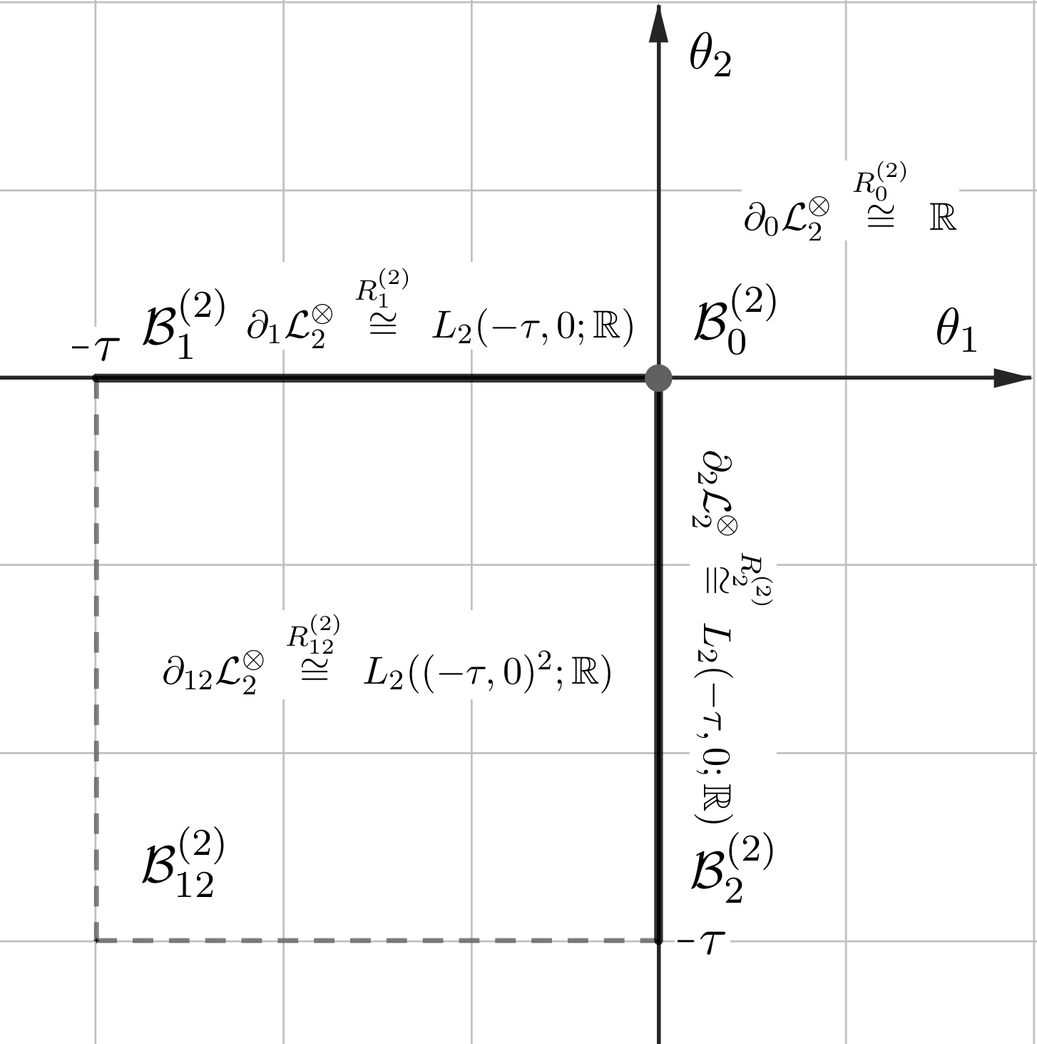
Refer to caption — Fig. 1: An illustration to the decomposition of $L_{2}([-\tau,0]^{2};\mu^{\otimes 2};\mathbb{R})$ according to (4.7), where the restriction operators $R^{(2)}_{0}$ , $R^{(2)}_{1}$ , $R^{(2)}_{2}$ , and $R^{(2)}_{12}$ provide natural isometric isomorphisms between the boundary subspaces over the faces $\mathcal{B}^{(2)}_{0}$ , $\mathcal{B}^{(2)}_{1}$ , $\mathcal{B}^{(2)}_{2}$ , and $\mathcal{B}^{(2)}_{12}$ and appropriate $L_{2}$ -spaces respectively.

For $m=2$ and $n=1$ , any element $\Phi\in\mathcal{L}^{\otimes}_{2}$ is determined by its four restrictions: $R^{(2)}_{0}\Phi\in\mathbb{R}$ , $R^{(2)}_{1}\Phi,R^{(2)}_{2}\Phi\in L_{2}(-\tau,0;\mathbb{R})$ , and $R^{(2)}_{12}\Phi\in L_{2}((-\tau,0)^{2};\mathbb{R})$ , see Fig. 1. Note that even if $R^{(2)}_{12}\Phi$ , $R^{(2)}_{1}\Phi$ , and $R^{(2)}_{2}\Phi$ have continuous representations, it is not necessary that they are somehow related on intersections of faces. For example, the values $(R^{(2)}_{12}\Phi)(0,0)$ , $(R^{(2)}_{1}\Phi)(0)$ , $(R^{(2)}_{2}\Phi)(0)$ , and $R^{(2)}_{0}\Phi$ need not be related.

Relations between restrictions arise for the elements of $\mathcal{L}^{\wedge}_{m}$ . This is contained in the following proposition. Recall here the operator $\Theta^{(m)}_{\sigma}$ defined in (2.16).

Proposition 4.1.

An element $\Phi\in\mathcal{L}^{\otimes}_{m}$ belongs to $\mathcal{L}^{\wedge}_{m}$ if and only if for all $k\in\{0,\ldots,m\}$ , integers $1\leq j_{1}<\cdots<j_{m}\leq m$ , and $\sigma\in\mathbb{S}_{m}$ , it satisfies

R_{j_{1}\ldots j_{k}}\Phi=(-1)^{\sigma}T_{\sigma}\Theta^{(k)}_{\bar{\sigma}}R_{\sigma(j_{1})\ldots\sigma(j_{k})}\Phi,

(4.8)

where $\bar{\sigma}\in\mathbb{S}_{k}$ is such that $\sigma(j_{\bar{\sigma}(1)})<\cdots<\sigma(j_{\bar{\sigma}(k)})$ .

As a consequence, we have that¹⁶¹⁶ 16 Here in (4.9) the tail of $\sigma$ , i.e., $\sigma(l)$ for $l\geq k+1$ is arbitrary.

R_{1\ldots k}\Phi=(-1)^{\sigma}T_{\sigma}R_{j_{1}\ldots j_{k}}\Phi\quad\text{for any}\quad\sigma=\begin{pmatrix}1&\ldots&k&\ldots\\ j_{1}&\ldots&j_{k}&\ldots\end{pmatrix}\in\mathbb{S}_{m},

(4.9)

and, in particular, for almost all $(\theta_{1},\ldots,\theta_{k})\in(-\tau,0)^{k}$ we have

(R_{1\ldots k}\Phi)(\theta_{1},\ldots,\theta_{k})\in(\mathbb{R}^{n})^{\otimes k}\otimes(\mathbb{R}^{n})^{\wedge(m-k)}.

(4.10)

Proof.

By Theorem 4.1, $\Phi\in\mathcal{L}^{\otimes}_{m}$ belongs to $\mathcal{L}^{\wedge}_{m}$ if and only if it is $\mu^{\otimes m}$ -antisymmetric, i.e., for any $\sigma\in\mathbb{S}_{m}$ we have

\Theta^{(m)}_{\sigma}\Phi=(-1)^{\sigma}T_{\sigma}\Phi\qquad\text{in}\quad\mathcal{L}^{\otimes}_{m}.

(4.11)

Applying the restriction operator $R_{j_{1}\ldots j_{k}}$ in (4.11), we obtain (4.8). For this, one should note the key identity

R_{j_{1}\ldots j_{k}}\Theta^{(m)}_{\sigma^{-1}}=\Theta^{(k)}_{\bar{\sigma}}R_{\sigma(j_{1})\ldots\sigma(j_{k})}.

(4.12)

Using the decomposition (4.7), we get that (4.8), taken over all restrictions, is the same as (4.11). This proves the necessity and sufficiency from the statement.

Note that (4.9) is a particular case of (4.8) with $j_{l}=l$ for $l\in\{1,\ldots,k\}$ .

To show (4.10), we use (4.9) with $j_{l}=l$ for $l\in\{1,\ldots,k\}$ and consider $\sigma$ such that

\sigma=\begin{pmatrix}1&\ldots&k&k+1&\ldots&m\\ 1&\ldots&k&\widetilde{\sigma}(1)+k&\ldots&\widetilde{\sigma}(m-k)+k\end{pmatrix},

(4.13)

where $\widetilde{\sigma}\in\mathbb{S}_{m-k}$ . Note that $(-1)^{\sigma}=(-1)^{\widetilde{\sigma}}$ . Summing (4.9) over all such $\widetilde{\sigma}$ and dividing by $(m-k)!$ , we obtain

R_{1\ldots k}\Phi=\left(\frac{1}{(m-k)!}\sum_{\widetilde{\sigma}\in\mathbb{S}_{m-k}}(-1)^{\widetilde{\sigma}}T_{\sigma}\right)R_{1\ldots k}\Phi

(4.14)

which shows (4.10). ∎

Since $\mathbb{R}^{\wedge k}=0$ for $k\geq 2$ , from Proposition 4.1 one may derive the following corollary, which is not technically important for what follows, and hence we left it for the reader as an exercise (or see [3, Proposition 4.2] for related arguments).

Corollary 4.1.

For $n=1$ , the relations from (4.8) are equivalent to the relations

$\displaystyle R_{j_{1}\ldots j_{k}}\Phi=0\qquad$	$\displaystyle\text{for all}\ k\in\{0,\ldots,m-2\},$
$\displaystyle R_{\hat{j}}\Phi\qquad$	$\displaystyle\text{is $\mu^{m-1}_{L}$-antisymmetric for any }j\in\{1,\ldots,m\},$	(4.15)
$\displaystyle R_{\hat{i}}\Phi=(-1)^{j-i}R_{\hat{j}}\Phi\qquad$	$\displaystyle\text{for}\ i,j\in\{1,\ldots,m\},$
$\displaystyle R_{1\ldots m}\Phi\qquad$	$\displaystyle\text{is $\mu^{m}_{L}$-antisymmetric}.$

Note that the antisymmetric relations (4.8) link each $\partial_{j_{1}\ldots j_{k}}\mathcal{L}^{\otimes}_{m}$ with other boundary subspaces over $k$ -faces. From this, it is convenient to define for a given $k\in\{0,\ldots,m\}$ the subspace (recall $\Pi^{\wedge}_{m}$ from (2.18))

\partial_{k}\mathcal{L}^{\wedge}_{m}\coloneq\left\{\Phi\in\bigoplus\limits_{j_{1}\ldots j_{k}}\partial_{j_{1}\ldots j_{k}}\mathcal{L}^{\otimes}_{m}\ |\ \Phi\text{ satisfies }\eqref{EQ: AntisymmetricRelationsGeneral}\right\}=\Pi^{\wedge}_{m}\bigoplus\limits_{j_{1}\ldots j_{k}}\partial_{j_{1}\ldots j_{k}}\mathcal{L}^{\otimes}_{m}.

(4.16)

Clearly, $\mathcal{L}^{\wedge}_{m}$ decomposes into the orthogonal sum of all $\partial_{k}\mathcal{L}^{\wedge}_{m}$ as follows:

\mathcal{L}^{\wedge}_{m}=\bigoplus_{k=0}^{m}\partial_{k}\mathcal{L}^{\wedge}_{m}.

(4.17)

An integer $k\in\{0,\ldots,m\}$ is called improper if $\partial_{k}\mathcal{L}^{\wedge}_{m}$ is the zero subspace. Otherwise $k$ is called proper. For $n=1$ , Corollary 4.1 shows that only $k=m-1$ and $k=m$ are proper. For general $n$ , (4.10) immediately yields that any $k<m-n$ is improper, since $(\mathbb{R}^{n})^{\wedge(m-k)}=\{0\}$ in this case. It can be shown that the inverse inequality $k\geq m-n$ implies that $k$ is proper (this is not essential for what follows).

Below, we consider some operators $A$ in $\mathbb{H}$ that arise in the study of delay equations and are therefore called delay operators. Their domain $\mathcal{D}(A)$ is given by the embedding¹⁷¹⁷ 17 Recall that the Sobolev space $W^{1,2}(-\tau,0;\mathbb{R}^{n})$ is continuously embedded into $C([-\tau,0];\mathbb{R}^{n})$ . of $W^{1,2}(-\tau,0;\mathbb{R}^{n})$ into $\mathbb{H}$ such that any $\psi\in W^{1,2}(-\tau,0;\mathbb{R}^{n})$ is mapped into $\phi\in\mathbb{H}$ satisfying $R^{(1)}_{0}\phi=\psi(0)$ and $R^{(1)}_{1}\phi=\psi$ . For $\phi\in\mathcal{D}(A)$ , the action of $A$ is defined as follows:

R^{(1)}_{0}(A\phi)=\widetilde{A}R^{(1)}_{1}\phi\quad\text{and}\quad R^{(1)}_{1}(A\phi)=\frac{d}{d\theta}R^{(1)}_{1}\phi,

(4.18)

where $\widetilde{A}\colon C([-\tau,0];\mathbb{R}^{n})\to\mathbb{R}^{n}$ is a bounded linear operator.

It can be shown that $A$ generates a $C_{0}$ -semigroup $G$ in $\mathbb{H}$ , see [7, 13]. We aim to describe the $m$ -fold additive compound $A^{[\otimes m]}$ of $A$ in $\mathbb{H}^{\otimes m}$ , discussed in Section 3, in terms of the space $\mathcal{L}^{\otimes}_{m}$ .

By the Riesz representation theorem, there exists an $(n\times n)$ -matrix function $\alpha(\cdot)$ of bounded variation on $[-\tau,0]$ such that

\widetilde{A}\phi=\int_{-\tau}^{0}d\alpha(\theta)\phi(\theta)\qquad\text{for any}\ \phi\in C([-\tau,0];\mathbb{R}^{n}).

(4.19)

For any integer $j\in\{1,\ldots,m\}$ , we set $\mathbb{R}_{1,j}\coloneq(\mathbb{R}^{n})^{\otimes(j-1)}$ and $\mathbb{R}_{2,j}\coloneq(\mathbb{R}^{n})^{\otimes(m-j)}$ and define a linear operator $\alpha_{j}(\theta)$ on $(\mathbb{R}^{n})^{\otimes m}$ by $\alpha_{j}(\theta)\coloneq\operatorname{Id}_{\mathbb{R}_{1,j}}\otimes\alpha(\theta)\otimes\operatorname{Id}_{\mathbb{R}_{2,j}}$ . Clearly, $\alpha_{j}$ has bounded variation on $[-\tau,0]$ .

Next, for any integers $j\in\{1,\ldots,m\}$ , $k\in\{0,\ldots,m-1\}$ and $J\in\{1,\ldots,k+1\}$ , we define a linear operator $\widetilde{A}^{(k)}_{j,J}$ taking a function $\Phi$ from $C([-\tau,0]^{k+1};(\mathbb{R}^{n})^{\otimes m})$ to a function from $C([-\tau,0]^{k};(\mathbb{R}^{n})^{\otimes m})$ by

(\widetilde{A}^{(k)}_{j,J}\Phi)(\theta_{1},\ldots,\hat{\theta}_{J},\ldots\theta_{k+1})\coloneq\int_{-\tau}^{0}d\alpha_{j}(\theta_{J})\Phi(\theta_{1},\ldots,\theta_{k+1})

(4.20)

for all $(\theta_{1},\ldots,\hat{\theta}_{J},\ldots,\theta_{k+1})\in[-\tau,0]^{k}$ .

Given integers $j_{1},\ldots,j_{k}$ with $k\in\{0,\ldots,m-1\}$ and $j\notin\{j_{1},\ldots,j_{k}\}$ , we define an integer $J(j)=J(j;j_{1},\ldots,j_{k})$ such that $j$ is the $J(j)$ th element in the set $\{j,j_{1},\ldots,j_{k}\}$ arranged by increasing. We usually write $J(j)$ when $j_{1},\ldots,j_{k}$ should be understood from the context.

Theorem 4.2.

Let $A$ be a delay operator as in (4.18). Then its $m$ -fold additive compound $A^{[\otimes m]}$ acts on $\Phi\in\mathcal{D}(A)^{\odot m}$ as follows:

R_{j_{1}\ldots j_{k}}\left(A^{[\otimes m]}\Phi\right)=\sum_{l=1}^{k}\frac{\partial}{\partial\theta_{j_{l}}}R_{j_{1}\ldots j_{k}}\Phi+\sum_{j\notin\{j_{1},\ldots,j_{k}\}}\widetilde{A}^{(k)}_{j,J(j)}R_{jj_{1}\ldots j_{k}}\Phi

(4.21)

for all $k\in\{0,\ldots,m\}$ and $1\leq j_{1}<\cdots<j_{k}\leq m$ . Here $R_{j_{1}\ldots j_{k}}\Phi$ is considered as a function of $(\theta_{j_{1}},\ldots,\theta_{j_{k}})\in(-\tau,0)^{k}$ .

Proof.

Due to linearity, it suffices to check (4.21) on decomposable tensors $\Phi=\phi_{1}\otimes\cdots\otimes\phi_{m}$ with $\phi_{j}\in\mathcal{D}(A)$ for $j\in\{1,\ldots,m\}$ . Here (3.5) is read as

A^{[\otimes m]}\Phi=\sum_{j=1}^{m}\phi_{1}\otimes\cdots\otimes A\phi_{j}\otimes\cdots\otimes\phi_{m}.

(4.22)

Using (4.18) and (4.6), it is straightforward to verify that

\begin{split}\left(R_{j_{1}\ldots j_{k}}(\phi_{1}\otimes\cdots\otimes A\phi_{j}\otimes\cdots\otimes\phi_{m})\right)(\theta_{j_{1}},\ldots,\theta_{j_{k}})=\\ =\begin{cases}\frac{d}{d\theta_{j}}(R_{j_{1}\ldots j_{k}}\Phi)(\theta_{j_{1}},\ldots,\theta_{j_{k}})\qquad&\text{if}\quad j\in\{j_{1},\ldots,j_{k}\},\\ \left(\widetilde{A}^{(k)}_{j,J(j)}R_{jj_{1}\ldots j_{k}}\Phi\right)(\theta_{j_{1}},\ldots,\theta_{j_{k}})\qquad&\text{if}\quad j\notin\{j_{1},\ldots,j_{k}\}\end{cases}\end{split}

(4.23)

for almost all $(\theta_{j_{1}},\ldots,\theta_{j_{k}})\in(-\tau,0)^{k}$ . Since $R_{j_{1}\ldots j_{k}}$ is linear, this gives (4.21). ∎

We will now characterize the domain $\mathcal{D}(A^{[\otimes m]})$ of $A^{[\otimes m]}$ and discuss in what sense the action (4.21) can be understood for general $\Phi\in\mathcal{D}(A^{[\otimes m]})$ , see Remark 4.3. For this, we recall the diagonal Sobolev space $\mathcal{W}^{2}_{D}(\Omega;\mathbb{F})$ from (A.4), which will be used with $\mathbb{F}=(\mathbb{R}^{n})^{\otimes m}$ and $\Omega=(-\tau,0)^{k}$ for $k\in\{1,\ldots,m\}$ . Based on its characterization given in Proposition A.1, we use the equivalent norm (A.21), denoted by $\|\cdot\|_{\mathcal{W}^{2}_{D}(\Omega;\mathbb{F})}$ . Recall also that on $\mathcal{W}^{2}_{D}((-\tau,0)^{k};(\mathbb{R}^{n})^{\otimes m})$ there is a well-defined trace operator $\operatorname{Tr}_{\mathcal{B}^{(k)}_{\hat{l}}}$ given by Theorem A.2 for each $l\in\{1,\ldots,k\}$ .

In the following theorem, we show that restrictions of any $\Phi\in\mathcal{D}(A^{[\otimes m]})$ belong to appropriate diagonal Sobolev spaces, and their traces agree with the restrictions of lower orders, see (4.24).

Theorem 4.3.

For any $\Phi\in\mathcal{D}(A^{[\otimes m]})$ , $k\in\{1,\ldots,m\}$ , and $1\leq j_{1}<\cdots<j_{k}\leq m$ , the restriction $R_{j_{1}\ldots j_{k}}\Phi$ belongs to $\mathcal{W}^{2}_{D}((-\tau,0)^{k};(\mathbb{R}^{n})^{\otimes m})$ and satisfies the identity¹⁸¹⁸ 18 Recall that $\bar{\theta}_{\hat{l}}$ is the vector obtained from $\bar{\theta}$ by omitting the $l$ th component.

\left(\operatorname{Tr}_{\mathcal{B}^{(k)}_{\hat{l}}}R_{j_{1}\ldots j_{k}}\Phi\right)(\bar{\theta})=(R_{j_{1}\ldots\hat{j_{l}}\ldots j_{k}}\Phi)(\bar{\theta}_{\hat{l}})

(4.24)

for $\mu^{k-1}_{L}$ -almost all $\bar{\theta}=(\theta_{1},\ldots,\theta_{k})\in\mathcal{B}^{(k)}_{\hat{l}}$ and each $l\in\{1,\ldots,k\}$ .

Furthermore, the norm $\|\cdot\|_{\mathcal{W}^{2}_{D}}$ on $\mathcal{D}(A^{[\otimes m]})$ given by

\|\Phi\|^{2}_{\mathcal{W}^{2}_{D}}\coloneq\sum_{k=1}^{m}\sum_{j_{1}\ldots j_{k}}\|R_{j_{1}\ldots j_{k}}\Phi\|^{2}_{\mathcal{W}^{2}_{D}((-\tau,0)^{k};(\mathbb{R}^{n})^{\otimes m})}

(4.25)

is equivalent to the graph norm.

Proof.

By Theorem 3.1, $\mathcal{D}(A)^{\odot m}$ is dense in $\mathcal{D}(A^{[\otimes m]})$ in the graph norm. Proposition A.1 gives that any $\Phi\in\mathcal{D}(A)^{\odot m}$ satisfies $R_{j_{1}\ldots j_{k}}\Phi\in\mathcal{W}^{2}_{D}((-\tau,0)^{k};(\mathbb{R}^{n})^{\otimes m})$ for any $j_{1}\ldots j_{k}$ as in the statement.

Note that the operator $\widetilde{A}^{(k)}_{j,J(j)}$ from (4.21) is the operator $C^{\gamma}_{J}$ from Theorem A.3 with $\gamma\coloneq\alpha_{j}$ defined below (4.19), $\mathbb{F}=\mathbb{M}_{\gamma}\coloneq(\mathbb{R}^{n})^{\otimes m}$ , and $J=J(j)$ . Using this and Proposition A.2, we can rewrite (4.21) as

\sum_{l=1}^{k}\frac{\partial}{\partial\theta_{j_{l}}}R_{j_{1}\ldots j_{k}}\Phi=R_{j_{1}\ldots j_{k}}\left(A^{[\otimes m]}\Phi\right)-\sum_{j\notin\{j_{1},\ldots,j_{k}\}}\widetilde{A}^{(k)}_{j,J(j)}R_{jj_{1}\ldots j_{k}}\Phi

(4.26)

and estimate the diagonal derivative of $R_{j_{1}\ldots j_{k}}\Phi$ . This gives for some constant $C(k)>0$ , which depends on $k$ , $\tau$ and the total variation $\operatorname{Var}_{[-\tau,0]}(\alpha)$ of $\alpha$ on $[-\tau,0]$ , the estimate

\begin{split}\|R_{j_{1}\ldots j_{k}}\Phi\|_{\mathcal{W}^{2}_{D}((-\tau,0)^{k};(\mathbb{R}^{n})^{\otimes m})}\leq\\ \leq C(k)\cdot\left(\|\Phi\|_{A^{[\otimes m]}}+\sum_{j\notin\{j_{1},\ldots,j_{k}\}}\|R_{jj_{1}\ldots j_{k}}\Phi\|_{\mathcal{W}^{2}_{D}((-\tau,0)^{k+1};(\mathbb{R}^{n})^{\otimes m})}\right),\end{split}

(4.27)

where $\|\cdot\|_{A^{[\otimes m]}}$ is the graph norm.

Clearly, $C(m)$ in (4.27) can be taken equal to $1$ . Thus, we have

\|R_{1\ldots m}\Phi\|_{\mathcal{W}^{2}_{D}((-\tau,0)^{m};(\mathbb{R}^{n})^{\otimes m})}\leq\|\Phi\|_{A^{[\otimes m]}}.

(4.28)

From this and (4.27), acting by induction from $k=m$ to $k=1$ , we obtain that the graph norm on $\mathcal{D}(A)^{\odot m}$ is stronger than $\|\cdot\|_{\mathcal{W}_{D}}$ . Similarly, we can apply Theorem A.3 and Proposition A.2 to estimate the $L_{2}$ -norm of $R_{j_{1}\ldots j_{k}}\left(A^{[\otimes m]}\Phi\right)$ from (4.26), thereby establishing that $\|\cdot\|_{\mathcal{W}^{2}_{D}}$ is stronger than the graph norm. Thus, both norms are equivalent on $\mathcal{D}(A)^{\odot m}$ and, consequently, $\mathcal{D}(A^{[\otimes m]})$ is determined by the completion by either of them.

Clearly, (4.24) is satisfied for $\Phi\in\mathcal{D}(A)^{\odot m}$ . Since trace operators on diagonal Sobolev spaces are bounded, (4.24) is satisfied for all $\Phi\in\mathcal{D}(A^{[\otimes m]})$ , due to the continuity and equivalence of norms. ∎

Remark 4.2.

In fact, $\mathcal{D}(A^{[\otimes m]})$ is characterized by the property described in Theorem 4.3. Namely, if $\Phi\in\mathcal{L}^{\otimes}_{m}$ satisfies $R_{j_{1}\ldots j_{k}}\Phi\in\mathcal{W}^{2}_{D}((-\tau,0)^{k};(\mathbb{R}^{n})^{\otimes m})$ and (4.24) for any $j_{1}\ldots j_{k}$ as in the statement, then it belongs to $\mathcal{D}(A^{[\otimes m]})$ . This result is not essential for the present and even our adjacent works, and therefore we will limit ourselves to only indicating the idea of the proof. Namely, since $\mathcal{D}(A^{[\otimes m]})$ does not depend¹⁹¹⁹ 19 Because $\mathcal{D}(A)^{\odot m}$ and the equivalent norm (4.25) do not depend on $\widetilde{A}$ . on $\widetilde{A}$ , it is sufficient to consider the case $\widetilde{A}=0$ . Here, we can explicitly construct the corresponding classical solutions by using Remark 5.2, where the converse to the structural Cauchy formula is discussed.

Remark 4.3.

Thus, any $\Phi\in\mathcal{D}(A^{[\otimes m]})$ has restrictions with $L_{2}$ -summable diagonal derivatives, and on such restrictions the action of $\widetilde{A}^{(k)}_{j,J(j)}$ can be extended according to Theorem A.3. In this sense, (4.21) can be understood for general $\Phi\in\mathcal{D}(A^{[\otimes m]})$ .

We now describe a property of the resolvent of $A^{[\otimes m]}$ that is crucial for studying spectral perturbations. For this, recall the spaces $\mathbb{E}^{2}_{k}(\mathbb{F})$ from Appendix A for $k\in\{1,\ldots,m\}$ and $\mathbb{F}=(\mathbb{R}^{n})^{\otimes m}$ , see near (A.32). Below, we also set $\mathbb{E}^{2}_{0}((\mathbb{R}^{n})^{\otimes m})\coloneq(\mathbb{R}^{n})^{\otimes m}$ . We define the Banach space $\mathbb{E}^{\otimes}_{m}$ through the outer direct sum as follows:

\mathbb{E}^{\otimes}_{m}\coloneq\bigoplus_{k=0}^{m}\bigoplus_{j_{1}\ldots j_{k}}\mathbb{E}^{2}_{k}((\mathbb{R}^{n})^{\otimes m}),

(4.29)

and endow it with any of standard norms. By naturally sending each element from the $j_{1}\ldots j_{k}$ th summand in (4.29) to $\partial_{j_{1}\ldots j_{k}}\mathcal{L}^{\otimes}_{m}$ , we embed the space $\mathbb{E}^{\otimes}_{m}$ into $\mathcal{L}^{\otimes}_{m}$ . From Proposition A.2 and Theorem 4.3 it follows that²⁰²⁰ 20 Instead of $\mathbb{E}^{\otimes}_{m}$ , we may also consider its subspace, where an analog of (4.24) is satisfied, namely, all restrictions agree with appropriate functions of $j$ th sections, see (A.31). By Theorem 4.3, we are in fact working in this subspace when considering the resolvents below. It is also clear that the embedding of $\mathcal{D}(A^{[\otimes m]})$ into this subspace is dense and continuous.

\mathcal{D}(A^{[\otimes m]})\subset\mathbb{E}^{\otimes}_{m}\subset\mathcal{L}^{\otimes}_{m},

(4.30)

where all the embeddings are continuous and dense in $\mathcal{L}^{\otimes}_{m}$ .

In the following theorem, there is a slight abuse of notation, since we are dealing with resolvents defined on complexifications of the spaces. For convenience, we omit mention of the complexifications, but it should be understood that all the spaces involved are complex, i.e., consist of $(\mathbb{C}^{n})^{\otimes m}$ -valued functions.

Theorem 4.4.

Let $p\in\mathbb{C}$ be a regular point of $A^{[\otimes m]}$ , i.e., $p\notin\operatorname{spec}(A^{[\otimes m]})$ . Then

\|(A^{[\otimes m]}-pI)^{-1}\|_{\mathcal{L}(\mathcal{L}^{\otimes}_{m};\mathbb{E}^{\otimes}_{m})}\leq C_{1}(p)\cdot\|(A^{[\otimes m]}-pI)^{-1}\|_{\mathcal{L}(\mathcal{L}^{\otimes}_{m})}+C_{2}(p),

(4.31)

where the constants $C_{1}(p)$ and $C_{2}(p)$ depend on $\max\{1,e^{-\tau\operatorname{Re}p}\}$ , $\tau$ , $m$ , and $\operatorname{Var}_{[-\tau,0]}(\alpha)$ in a monotonically increasing manner. Furthermore, a similar statement is valid for regular points of $A^{[\wedge m]}$ .

Proof.

Suppose $(A^{[\otimes m]}-pI)\Phi=\Psi$ for some $\Psi\in\mathcal{L}^{\otimes}_{m}$ and $\Phi\in\mathcal{D}(A^{[\otimes m]})$ . From Theorem 4.3 we get that $R_{j_{1}\ldots j_{k}}\Phi\in\mathcal{W}^{2}_{D}((-\tau,0)^{k};(\mathbb{C}^{n})^{\otimes m})$ for any $k\in\{1,\ldots,m\}$ and $1\leq j_{1}<\cdots j_{k}\leq m$ . We have to estimate the norm of $R_{j_{1}\ldots j_{k}}\Phi$ in $\mathbb{E}^{2}_{k}((\mathbb{C}^{n})^{\otimes m})$ . This will be done by induction from $k=m$ to $k=1$ .

For $k=m$ , we consider $\bar{\theta}\in\mathcal{B}^{(m)}_{\hat{j}}$ for some $j\in\{1,\ldots,m\}$ and define $D_{\bar{\theta}}\coloneq(-\tau,0)^{m}\cap(\mathcal{L}_{0}+\bar{\theta})$ , where $\mathcal{L}_{0}=\{\underline{t}\in\mathbb{R}^{m}\ |\ t\in\mathbb{R}\}$ is the diagonal line in $\mathbb{R}^{m}$ . Assuming $\bar{\theta}=(\theta_{1},\ldots,\theta_{m})$ , we set $\tau(\bar{\theta})\coloneq\tau+\min_{1\leq l\leq m}\theta_{l}$ . Then the closure of $D_{\bar{\theta}}$ consist of points $\bar{\theta}+\zeta\cdot\underline{1}$ , where $\underline{1}=(1,\ldots,1)\in\mathbb{R}^{m}$ and $\zeta\in[-\tau(\bar{\theta}),0]$ .

Then for $\mu^{m-1}_{L}$ -almost all $\bar{\theta}\in\mathcal{B}^{(m)}_{\hat{j}}$ we have that ${\left.\kern-1.2ptR_{1\ldots m}\Phi\vphantom{\big|}\right|_{D_{\bar{\theta}}}}$ is well defined and can be considered as an element of $W^{1,2}(-\tau(\bar{\theta}),0;(\mathbb{C}^{n})^{\otimes m})$ . In these terms, (4.21) gives

\begin{split}\frac{d}{d\zeta}{\left.\kern-1.2ptR_{1\ldots m}\Phi\vphantom{\big|}\right|_{D_{\bar{\theta}}}}-p{\left.\kern-1.2ptR_{1\ldots m}\Phi\vphantom{\big|}\right|_{D_{\bar{\theta}}}}={\left.\kern-1.2ptR_{1\ldots m}\Psi\vphantom{\big|}\right|_{D_{\bar{\theta}}}}.\end{split}

(4.32)

Applying the Cauchy formula, for any $\zeta\in(-\tau(\bar{\theta}),0)$ we obtain

{\left.\kern-1.2ptR_{1\ldots m}\Phi\vphantom{\big|}\right|_{D_{\bar{\theta}}}}(\zeta)=e^{p\zeta}{\left.\kern-1.2ptR_{1\ldots m}\Phi\vphantom{\big|}\right|_{D_{\bar{\theta}}}}(0)-\int_{\zeta}^{0}e^{p(\zeta-s)}{\left.\kern-1.2ptR_{1\ldots m}\Psi\vphantom{\big|}\right|_{D_{\bar{\theta}}}}(s)ds.

(4.33)

This and the Hölder inequality yield the estimate

\begin{split}\left|{\left.\kern-1.2ptR_{1\ldots m}\Phi\vphantom{\big|}\right|_{D_{\bar{\theta}}}}(\zeta)\right|\leq\\ \leq C_{0}(p)\cdot\left(\left|\Phi(\bar{\theta})\right|+\left\|{\left.\kern-1.2ptR_{1\ldots m}\Psi\vphantom{\big|}\right|_{D_{\bar{\theta}}}}\right\|_{L_{2}(D_{\bar{\theta}};(\mathbb{C}^{n})^{\otimes m})}\right),\end{split}

(4.34)

where $C_{0}(p)=\max\{1,\sqrt{\tau}\}\cdot\max\{1,e^{-\tau\operatorname{Re}p}\}$ and $|\cdot|$ denotes the norm in $(\mathbb{C}^{n})^{\otimes m}$ .

By combining the above estimates for any $j\in\{1,\ldots,m\}$ , we get for any $l\in\{1,\ldots,m\}$ and all $\theta\in[-\tau,0]$ in appropriate $L_{2}$ -norms the estimate²¹²¹ 21 Here $e_{l}$ is the $l$ th vector from the standard basis in $\mathbb{R}^{m}$ .

\left\|\operatorname{Tr}_{\mathcal{B}^{(m)}_{\hat{l}}+\theta e_{l}}\Phi\right\|_{L_{2}}\leq\widetilde{C}_{0}(p)\cdot\left(\sum_{j=1}^{m}\|R_{\hat{j}}\Phi\|_{L_{2}}+\|R_{1\ldots m}\Psi\|_{L_{2}}\right),

(4.35)

where $\widetilde{C}_{0}(p)$ equals $C_{0}(p)$ multiplied by an absolute constant.

From the Cauchy inequality and since $p$ is a regular point, we have

\sum_{j=1}^{m}\|R_{\hat{j}}\Phi\|_{L_{2}}\leq\sqrt{m}\cdot\|\Phi\|_{\mathcal{L}^{\otimes}_{m}}\leq\sqrt{m}\cdot\|(A^{[\otimes m]}-pI)^{-1}\|_{\mathcal{L}(\mathcal{L}^{\otimes}_{m})}\cdot\|\Psi\|_{\mathcal{L}^{\otimes}_{m}}.

(4.36)

Now, combining (4.35) and (4.36), we get

\begin{split}\|R_{1\ldots m}\Phi\|_{\mathbb{E}^{2}_{m}((\mathbb{C}^{n})^{\otimes m})}=\sup_{l\in\{1,\ldots,m\}}\sup_{\theta\in[-\tau,0]}\left\|\operatorname{Tr}_{\mathcal{B}^{(m)}_{\hat{l}}+\theta e_{l}}\Phi\right\|_{L_{2}}\leq\\ \leq(\sqrt{m}\cdot\widetilde{C}_{0}(p)\cdot\|(A^{[\otimes m]}-pI)^{-1}\|_{\mathcal{L}(\mathcal{L}^{\otimes}_{m})}+1)\cdot\|\Psi\|_{\mathcal{L}^{\otimes}_{m}}.\end{split}

(4.37)

This is the required estimate for $k=m$ .

Now consider $k\in\{0,\ldots,m-1\}$ and $1\leq j_{1}<\cdots<j_{k}\leq m$ , assuming that the statement has already been proved for larger $k$ . Given $j\in\{1,\ldots,k\}$ , for any $\bar{\theta}\in\mathcal{B}^{(k)}_{\hat{j}}$ we similarly define $D_{\bar{\theta}}\coloneq(-\tau,0)^{k}\cap(\mathcal{L}_{0}+\bar{\theta})$ , where $\mathcal{L}_{0}=\{\underline{t}\in\mathbb{R}^{k}\ |\ t\in\mathbb{R}\}$ is the diagonal line in $\mathbb{R}^{k}$ . Here an analog of (4.32), which is also derived from (4.21), is given by

\begin{split}\frac{d}{d\zeta}{\left.\kern-1.2ptR_{j_{1}\ldots j_{k}}\Phi\vphantom{\big|}\right|_{D_{\bar{\theta}}}}-p{\left.\kern-1.2ptR_{j_{1}\ldots j_{k}}\Phi\vphantom{\big|}\right|_{D_{\bar{\theta}}}}=\\ =-\sum_{j\notin\{j_{1},\ldots,j_{k}\}}{\left.\kern-1.2pt(\widetilde{A}^{(k)}_{j,J(j)}R_{jj_{1}\ldots j_{k}}\Phi)\vphantom{\big|}\right|_{D_{\bar{\theta}}}}+{\left.\kern-1.2ptR_{j_{1}\ldots j_{k}}\Psi\vphantom{\big|}\right|_{D_{\bar{\theta}}}}.\end{split}

(4.38)

By applying the Cauchy formula, one obtains an analog of (4.35) in appropriate $L_{2}$ -spaces for each $l\in\{1,\ldots,k\}$ as follows:

\begin{split}\left\|\operatorname{Tr}_{\mathcal{B}^{(k)}_{\hat{l}}+\theta e_{l}}\Phi\right\|_{L_{2}}\leq\widetilde{C}_{0}(p)\cdot\Biggl(\|R_{j_{1}\ldots j_{k}}\Psi\|_{L_{2}}+\sum_{l=1}^{k}\|R_{j_{1}\ldots\hat{j_{l}}\ldots j_{k}}\Phi\|_{L_{2}}+\\ +\sum_{j\notin\{j_{1}\ldots j_{k}\}}\|\widetilde{A}^{(k)}_{j,J(j)}R_{jj_{1}\ldots j_{k}}\Phi\|_{L_{2}}\Biggr),\end{split}

(4.39)

where $e_{l}$ is the $l$ th basis vector in the standard basis of $\mathbb{R}^{k}$ , and $\widetilde{C}_{0}(p)$ can be taken the same.

Note that we already have an upper estimate for the $L_{2}$ -norm of the new (last) term in (4.39), since Theorem A.3 provides an estimate²²²² 22 See above (4.26) for details. for the $j$ th summand in terms of the norm of $R_{jj_{1}\ldots j_{k}}\Phi$ in $\mathbb{E}^{2}_{k+1}((\mathbb{C}^{n})^{\otimes m})$ , which can be further estimated from the previous step. Furthermore, similarly to (4.37), the resulting estimates are always of the form

\begin{split}\|R_{j_{1}\ldots j_{k}}\Phi\|_{\mathbb{E}_{k}((\mathbb{C}^{n})^{\otimes m})}\leq\\ \leq C^{(k)}_{1}(p)\cdot\|(A^{[\otimes m]}-pI)^{-1}\|_{\mathcal{L}(\mathcal{L}^{\otimes}_{m})}\cdot\|\Psi\|_{\mathcal{L}^{\otimes}_{m}}+C^{(k)}_{2}(p)\cdot\|\Psi\|_{\mathcal{L}^{\otimes}_{m}},\end{split}

(4.40)

where the constants $C^{(k)}_{1}(p)$ and $C^{(k)}_{2}(p)$ are formed from the previous ones by addition and multiplication of $\widetilde{C}_{0}(p)$ , $\sqrt{m}$ , $\sqrt{\tau}$ , $\operatorname{Var}_{[-\tau,0]}(\alpha)$ , and some absolute constants. This shows the monotone behavior of $C_{1}(p)$ and $C_{2}(p)$ from the statement.

It should also be noted that we only used the existence of the resolvent of $A^{[\otimes m]}$ , and hence the same estimates hold for $A^{[\wedge m]}$ and its regular points $p$ if we take $\Psi\in\mathcal{L}^{\wedge}_{m}$ . ∎

Remark 4.4.

In contrast to the case $m=1$ , the resolvent of $A^{[\wedge m]}$ (and, hence, $A^{[\otimes m]}$ ) ceases to be compact for $m>1$ . In other words, the embedding of $\mathcal{D}(A^{[\wedge m]})$ into $\mathcal{L}^{\wedge}_{m}$ is not compact. Let us illustrate²³²³ 23 In particular, the below arguments show that the embedding of the diagonal Sobolev space over $(-\tau,0)^{m}$ into $L_{2}$ is not compact for $m>1$ , which is more obvious. this in the case $m=2$ and $n=1$ . For any positive integer $k$ , consider $\Phi_{k}(\theta_{1},\theta_{2})\coloneq\sin(\frac{2\pi k}{\tau}(\theta_{1}-\theta_{2}))$ . Note that $\Phi_{k}$ can be viewed as an element $\Psi_{k}$ of $\mathcal{D}(A^{[\wedge 2]})$ with $R_{12}\Psi_{k}=\Phi_{k}$ , $R_{1}\Psi_{k}=-R_{2}\Psi_{k}=\Phi_{k}(\cdot,0)$ , and $R_{0}\Psi_{k}=0$ . Clearly, we have

\left(\frac{\partial}{\partial\theta_{1}}+\frac{\partial}{\partial\theta_{2}}\right)\Phi_{k}(\theta_{1},\theta_{2})\equiv 0\qquad\text{for}\ (\theta_{1},\theta_{2})\in(-\tau,0)^{2}.

(4.41)

Moreover, $R_{12}\Psi_{k}$ and $R_{12}\Psi_{l}$ are orthogonal in $L_{2}$ for $k\not=l$ . However, the boundary values of $\Phi_{k}$ make the family of $\Psi_{k}$ unbounded in the graph norm. To overcome this, we use a proper truncation of $\Phi_{k}$ . Given $\varepsilon>0$ , let $c=c(\theta_{1},\theta_{2})$ be a scalar $C^{1}$ -function of $(\theta_{1},\theta_{2})\in[-\tau,0]^{2}$ such that²⁴²⁴ 24 Such a function can be defined on segments parallel to the diagonal line by properly scaling the truncation function on $[0,1]$ , which equals to $1$ everywhere except a small neighborhood of $1$ , where it decays to zero.

1).

$c(\theta_{1},\theta_{2})=c(\theta_{2},\theta_{1})$ ;
2).

The diagonal derivative $(\frac{\partial}{\partial\theta_{1}}+\frac{\partial}{\partial\theta_{2}})c(\theta_{1},\theta_{2})$ is bounded;
3).

$c(\theta_{1},0)=c(0,\theta_{2})=0$ ;
4).

$0\leq c(\theta_{1},\theta_{2})\leq 1$ everywhere and $c(\theta_{1},\theta_{2})\not=1$ on a set of measure $\leq\varepsilon$ .

Then we set $\Phi_{\varepsilon,k}\coloneq c\cdot\Phi_{k}$ . From (4.41) we obtain that

\left(\frac{\partial}{\partial\theta_{1}}+\frac{\partial}{\partial\theta_{2}}\right)\Phi_{\varepsilon,k}(\theta_{1},\theta_{2})=\Phi_{k}(\theta_{1},\theta_{2})\left(\frac{\partial}{\partial\theta_{1}}+\frac{\partial}{\partial\theta_{2}}\right)c(\theta_{1},\theta_{2}).

(4.42)

Item 3) ensures that the boundary values of $\Phi_{\varepsilon,k}$ are zero, and hence from (4.42) and items 1), 2), and 4) we get that the family of all $\Psi_{\varepsilon,k}$ such that $R_{12}\Psi_{\varepsilon,k}=\Phi_{\varepsilon,k}$ , $R_{1}\Psi_{\varepsilon,k}=-R_{2}\Psi_{\varepsilon,k}=\Phi_{\varepsilon,k}(\cdot,0)$ , and $R_{0}\Psi_{\varepsilon,k}=0$ belongs to $\mathcal{D}(A^{[\wedge 2]})$ and bounded in the graph norm for a fixed $\varepsilon$ . Furthermore, according to the definition of $\Phi_{k}$ and item 4), there exists $\delta>0$ such that the inequality

\|\Phi_{\varepsilon,k}-\Phi_{\varepsilon,l}\|_{L_{2}((-\tau,0)^{2};\mathbb{R})}\geq\delta\text{ for any }k\not=l.

(4.43)

is satisfied for all sufficiently small $\varepsilon>0$ . In particular, one cannot extract a convergent in $L_{2}$ subsequence from $\Phi_{\varepsilon,k}$ . This shows that the resolvent of $A^{[\wedge 2]}$ is not compact.

Remark 4.5.

In the applications discussed in Section 6, we are interested in transfer operators associated with $A^{[\wedge m]}$ , and these are related to the boundary action of the resolvent, i.e., the correspondence $\Psi\mapsto\Phi$ , where $\Phi=(A^{[\wedge m]}-pI)^{-1}\Psi$ and $\Psi\in\mathcal{L}^{\wedge}_{m}$ satisfies $R_{1\ldots m}\Psi=0$ . From (4.21) it is seen that in this case $R_{1\ldots m}\Phi$ is determined from the restrictions of lower order. In particular, for $m=2$ , the entire $\Phi$ is determined from $R_{1}\Phi=-R_{2}\Phi$ and $R_{0}\Phi$ . Since $R_{1}\Phi$ belongs to the usual Sobolev space $W^{1,2}(-\tau,0;(\mathbb{C}^{n})^{\otimes m})$ , which compactly embeds into $C([-\tau,0];(\mathbb{C}^{n})^{\otimes m})$ , the boundary action $\Psi\mapsto\Phi\in\mathbb{E}^{\otimes}_{2}$ is a compact operator. Furthermore, at least in the single delay case, i.e., when $\widetilde{A}$ in (4.18) is given by $\widetilde{A}\phi=A_{0}\phi(0)+A_{-\tau}\phi(-\tau)$ for some $(n\times n)$ -matrices $A_{0}$ and $A_{-\tau}$ , we know (see [3, Section 4.5] for $n=1$ ) that the boundary action is an integral operator with an $L_{2}$ -summable kernel and expect this to hold in a wider generality. Thus, the case $m=2$ is special for computations.

We finalize this section by describing the spectra of $A^{[\otimes m]}$ and $A^{[\wedge m]}$ . It is well known that the semigroup $G$ generated by $A$ is eventually compact, see [7]. Consequently, Theorems 3.2 and 3.3 are applicable and yield the following.

Proposition 4.2.

For any delay operator $A$ given by (4.18), all conclusions of Theorems 3.2 and 3.3 are valid.

5 Structural Cauchy formula for linear inhomogeneous problems

Let $A$ be the delay operator given by (4.18). Recall that it acts in the Hilbert space $\mathbb{H}$ from (4.1). In this section, we consider the $m$ -fold additive compound $A^{[\otimes m]}$ of $A$ as an operator in the space $\mathcal{L}^{\otimes}_{m}$ from (4.3), as described in Theorems 4.2 and 4.3.

We are going to study structural properties of solutions to the linear inhomogeneous evolutionary system in $\mathcal{L}^{\otimes}_{m}$ :

\dot{\Phi}(t)=(A^{[\otimes m]}+\nu I)\Phi(t)+\eta(t),

(5.1)

where $I$ denotes the identity operator in $\mathcal{L}^{\otimes}_{m}$ , $\nu\in\mathbb{R}$ is fixed, and $\eta(\cdot)\in L_{2}(0,T;\mathcal{L}^{\otimes}_{m})$ for some $T>0$ .

Recall the $C_{0}$ -semigroup $G^{\otimes m}$ generated by $A^{[\otimes m]}$ and its time- $t$ mappings $G^{\otimes m}(t)$ , where $t\geq 0$ . Then for any $\Phi_{0}\in\mathcal{L}^{\otimes}_{m}$ there exists a unique mild solution $\Phi(t)=\Phi(t;\Phi_{0},\eta)$ to the Cauchy problem $\Phi(0)=\Phi_{0}$ for (5.1) on $[0,T]$ . It is delivered by the Cauchy formula

\Phi(t)=e^{\nu t}G^{\otimes m}(t)\Phi_{0}+\int_{0}^{t}e^{\nu(t-s)}G^{\otimes m}(t-s)\eta(s)ds.

(5.2)

For brevity, we will say that the pair $(\Phi(\cdot),\eta(\cdot))$ solves (5.1) on $[0,T]$ .

Remark 5.1.

Clearly, for any pair $(\Phi(t),\eta(t))=(\Phi_{\nu}(t),\eta_{\nu}(t))$ which solves (5.1) on $[0,T]$ , the pair $(e^{-\nu t}\Phi_{\nu}(t),e^{-\nu t}\eta_{\nu}(t))$ solves (5.1) with $\nu=0$ on $[0,T]$ .

Recall here the space $\mathcal{Y}^{2}_{\rho}(0,T;\mathbb{F})$ of $\rho$ -adorned $\mathbb{F}$ -valued functions on $[0,T]$ and the space $\mathcal{T}^{2}_{\rho}(0,T;\mathbb{F})$ of $\rho$ -twisted $\mathbb{F}$ -valued functions on $[0,T]$ , defined above (B.27) and (B.40), respectively. Below, we consider these spaces for $\rho(t)=\rho_{\nu}(t)\coloneq e^{\nu t}$ and $\mathbb{F}$ which is $L_{2}((-\tau,0)^{k};(\mathbb{R}^{n})^{\otimes m})$ for some $k\in\{1,\ldots,m\}$ .

Now we are ready to formulate the main result of this section, which is the cornerstone of the entire paper. This is the decomposition (5.3) of solutions to the linear inhomogeneous problem (5.1), which we call a structural Cauchy formula. Here, the interior and boundary parts of the solution are decomposed into the sum of $\rho_{\nu}$ -adorned and $\rho_{\nu}$ -twisted functions. Note that this decomposition is unique according to Proposition B.1. Moreover, the decomposition differs from (5.2) that can be seen from the fact that $\Phi_{X_{j_{1}\ldots j_{k}},\rho_{\nu}}$ in (5.3) depends on the entire solution $\Phi$ (and hence $\eta$ ) in general, see (5.26) for an explicit construction.

However, each formula (5.3), when properly read, is the usual Cauchy formula for a linear inhomogeneous problem associated with the generator $A_{T_{k}}$ of the diagonal translation semigroup $T_{k}$ in $L_{2}((-\tau,0)^{k};(\mathbb{R}^{n})^{\otimes m})$ given by Theorem A.4, see (5.27).

Theorem 5.1 (Structural Cauchy formula).

Suppose that $\nu\in\mathbb{R}$ , $T>0$ , $\Phi_{0}\in\mathcal{L}^{\otimes}_{m}$ , and $\eta_{\nu}(\cdot)\in L_{2}(0,T;\mathcal{L}^{\otimes}_{m})$ are given. Let $\Phi_{\nu}(\cdot)$ be the mild solution on $[0,T]$ to (5.1) with $\eta=\eta_{\nu}$ such that $\Phi_{\nu}(0)=\Phi_{0}$ . Then for any $k\in\{1,\ldots,m\}$ and $1\leq j_{1}<\cdots<j_{k}\leq m$ , there exist functions²⁵²⁵ 25 Here $\mathcal{C}^{k}_{T}$ is given by (B.22). $X_{j_{1}\ldots j_{k}}\in L_{2}(\mathcal{C}^{k}_{T};(\mathbb{R}^{n})^{\otimes m})$ and $Y_{j_{1}\ldots j_{k}}\in L_{2}(0,T;L_{2}((-\tau,0)^{k};(\mathbb{R}^{n})^{\otimes m}))$ such that $R_{j_{1}\ldots j_{k}}\Phi_{\nu}$ is the sum of the $\rho_{\nu}$ -adornment of $X_{j_{1}\ldots j_{k}}$ and the $\rho_{\nu}$ -twisting of $Y_{j_{1}\ldots j_{k}}$ for $\rho_{\nu}(t)\coloneq e^{\nu t}$ , i.e., in terms of (B.24) and (B.37), we have

R_{j_{1}\ldots j_{k}}\Phi_{\nu}(t)=\Phi_{X_{j_{1}\ldots j_{k}},\rho_{\nu}}(t)+\Psi_{Y_{j_{1}\ldots j_{k}},\rho_{\nu}}(t)\qquad\text{for all}\ t\in[0,T].

(5.3)

In particular, $R_{j_{1}\ldots j_{k}}\Phi_{\nu}$ belongs to the space $\mathcal{A}^{2}_{\rho_{\nu}}(0,T;L_{2}((-\tau,0)^{k};(\mathbb{R}^{n})^{\otimes m})$ of $\rho_{\nu}$ -agalmanated functions, see (B.57). Furthermore,

\begin{split}\rho_{\nu}(t)Y_{j_{1}\ldots j_{k}}(t)=\\ =R_{j_{1}\ldots j_{k}}\eta_{\nu}(t)+\sum_{j\notin\{j_{1},\ldots,j_{k}\}}\widetilde{A}^{(k)}_{j,J(j)}R_{jj_{1}\ldots j_{k}}\Phi_{\nu}(t)\qquad\text{for almost all}\ t\in[0,T],\end{split}

(5.4)

where $\widetilde{A}^{(k)}_{j,J(j)}$ as in (4.21), and its action is understood according to Theorem B.9.

In addition, for $\Phi_{0}\in\mathcal{D}(A^{[\otimes m]})$ and $\eta_{\nu}(\cdot)\in C^{1}([0,T];\mathcal{L}^{\otimes}_{m})$ , we have that²⁶²⁶ 26 Here $\mathring{\mathcal{C}}^{k}_{T}$ denotes the interior of $\mathcal{C}^{k}_{T}$ .

\begin{split}X_{j_{1}\ldots j_{k}}&\in\mathcal{W}^{2}_{D}(\mathring{\mathcal{C}}^{k}_{T};(\mathbb{R}^{n})^{\otimes m}),\\ \Phi_{X_{j_{1},\ldots,j_{k}},\rho_{\nu}}(\cdot)&\in C^{1}([0,T];L_{2})\cap C([0,T];\mathcal{W}^{2}_{D}),\\ \Psi_{Y_{j_{1}\ldots j_{k}},\rho_{\nu}}(\cdot)&\in C^{1}([0,T];L_{2})\cap C([0,T];\mathcal{W}^{2}_{D_{0}}),\end{split}

(5.5)

where $L_{2}$ stands for $L_{2}((-\tau,0)^{k};(\mathbb{R}^{n})^{\otimes m})$ , $\mathcal{W}^{2}_{D}$ stands for $\mathcal{W}^{2}_{D}((-\tau,0)^{k};(\mathbb{R}^{n})^{\otimes m})$ , and $\mathcal{W}^{2}_{D_{0}}$ stands for $\mathcal{W}^{2}_{D_{0}}((-\tau,0)^{k};(\mathbb{R}^{n})^{\otimes m})$ given by (A.38).

Before proving the theorem, we establish that $\Phi_{X_{j_{1}\ldots j_{k}},\rho_{\nu}}$ and $\Psi_{Y_{j_{1}\ldots j_{k}},\rho_{\nu}}$ in (5.3) must depend continuously on the data $(\Phi_{0},\eta_{\nu})$ from $\mathcal{L}^{\otimes}_{m}\times L_{2}(0,T;\mathcal{L}^{\otimes}_{m})$ . This will be done by deriving the estimate (5.6) in terms of the data and the solution $\Phi_{\nu}$ itself. For $T=\infty$ , the estimate will be considered in Section 6.3. Moreover, the proof introduces an explicit construction of $X_{j_{1}\ldots j_{k}}$ in (5.8) and (5.11), which will be used to prove Theorem 5.1.

For the following theorem, $\mathcal{Y}^{2}_{\rho_{\nu}}$ stands for $\mathcal{Y}^{2}_{\rho_{\nu}}(0,T;L_{2}((-\tau,0)^{k};(\mathbb{R}^{n})^{\otimes m}))$ , and $\mathcal{T}^{2}_{\rho_{\nu}}$ stands for $\mathcal{T}^{2}_{\rho_{\nu}}(0,T;L_{2}((-\tau,0)^{k};(\mathbb{R}^{n})^{\otimes m}))$ , where $T$ and $k$ are understood from the context.

Theorem 5.2.

In terms of Theorem 5.1, assume that the decompositions (5.3) and (5.4) and the property from (5.5) are valid for all $k\in\{1,\ldots,m\}$ and $1\leq j_{1}<\cdots<j_{k}\leq m$ . Then the norms $\|\Phi_{X_{j_{1}\ldots j_{k}},\rho_{\nu}}\|_{\mathcal{Y}^{2}_{\rho_{\nu}}}$ and $\|\Psi_{Y_{j_{1}\ldots j_{k}},\rho_{\nu}}\|_{\mathcal{T}^{2}_{\rho_{\nu}}}$ defined in (B.33) and (B.40), respectively, admit the estimate

\begin{split}\left\|\Phi_{X_{j_{1}\ldots j_{k}},\rho_{\nu}}\right\|^{2}_{\mathcal{Y}^{2}_{\rho_{\nu}}}+\left\|\Psi_{Y_{j_{1}\ldots j_{k}},\rho_{\nu}}\right\|^{2}_{\mathcal{T}^{2}_{\rho_{\nu}}}\leq\\ \leq C_{k}\cdot\left(|\Phi_{\nu}(0)|^{2}_{\mathcal{L}^{\otimes}_{m}}+\int_{0}^{T}|\Phi_{\nu}(t)|^{2}_{\mathcal{L}^{\otimes}_{m}}dt+\int_{0}^{T}|\eta_{\nu}(t)|^{2}_{\mathcal{L}^{\otimes}_{m}}dt\right),\end{split}

(5.6)

where the constant $C_{k}>0$ depends on $\max\{1,e^{\nu\tau}\}$ , $\tau$ , and the total variation $\operatorname{Var}_{[-\tau,0]}(\alpha)$ of $\alpha$ from (4.19) in a monotonically increasing manner and does not depend on $T$ .

Proof.

We give a proof by induction from $k=m$ to $k=1$ .

For $k=m$ , (5.4) reads as $\rho_{\nu}(t)Y_{1\ldots m}(t)=R_{1\ldots m}\eta_{\nu}(t)$ . Consequently,

\begin{split}\left\|\Psi_{Y_{1\ldots m},\rho_{\nu}}\right\|^{2}_{\mathcal{T}^{2}_{\rho_{\nu}}}\coloneq&\int_{0}^{T}\|\rho_{\nu}(t)Y_{1\ldots m}(t)\|^{2}_{L_{2}}dt=\\ =&\int_{0}^{T}\|R_{1\ldots m}\eta_{\nu}(t)\|^{2}_{L_{2}}dt\leq\int_{0}^{T}|\eta_{\nu}(t)|^{2}_{\mathcal{L}^{\otimes}_{m}}dt,\end{split}

(5.7)

where $L_{2}$ stands for $L_{2}((-\tau,0)^{m};(\mathbb{R}^{n})^{\otimes m})$ .

Now consider $\Phi_{0}\in\mathcal{D}(A^{[\otimes m]})$ and $\eta_{\nu}(\cdot)\in C^{1}([0,T];\mathcal{L}^{\otimes}_{m})$ . For such data, the solution $\Phi_{\nu}(\cdot)$ is classical, according to [26, Chapter I, Theorem 6.5], and, in particular, satisfies $\Phi_{\nu}(\cdot)\in C([0,T];\mathcal{D}(A^{[\otimes m]}))$ . Thanks to (5.5), for any $j\in\{1,\ldots,m\}$ we may apply the trace operator $\operatorname{Tr}_{\mathcal{B}^{(m)}_{\hat{j}}}$ given by Theorem A.2 to both sides of (5.3). From this, according to Theorem 4.3 and the definition of $\Phi_{X_{1\ldots m},\rho_{\nu}}$ in (B.24), we obtain

\begin{split}\rho_{\nu}(t)X_{1\ldots m}(\bar{\theta}+\underline{t})=(\operatorname{Tr}_{\mathcal{B}^{(m)}_{\hat{j}}}\Phi_{X_{1\ldots m},\rho_{\nu}}(t))(\bar{\theta})=\\ =(\operatorname{Tr}_{\mathcal{B}^{(m)}_{\hat{j}}}R_{1\ldots m}\Phi(t))(\bar{\theta})=R_{\hat{j}}\Phi_{\nu}(t)(\bar{\theta}_{\hat{j}})\end{split}

(5.8)

for almost all $t\in[0,T]$ and $\mu^{m-1}_{L}$ -almost all $\bar{\theta}\in\mathcal{B}^{(m)}_{\hat{j}}$ . From this, by applying the Fubini theorem in (B.27), we get

\begin{split}&\|\Phi_{X_{1\ldots m},\rho_{\nu}}\|^{2}_{\mathcal{Y}^{2}_{\rho_{\nu}}}=\\ &=\|R_{1\ldots m}\Phi_{0}\|^{2}_{L_{2}}+\int_{0}^{T}e^{2\nu t}\left(\sum_{j=1}^{m}\int_{\mathcal{B}_{\hat{j}}}|X_{1\ldots m}(\bar{\theta}+\underline{t})|^{2}d\mu^{m-1}_{L}(\bar{\theta})\right)dt=\\ &=\|R_{1\ldots m}\Phi_{0}\|^{2}_{L_{2}}+\int_{0}^{T}\sum_{j=1}^{m}\|R_{\hat{j}}\Phi_{\nu}(t)\|^{2}_{L_{2}}dt\leq\\ &\leq|\Phi_{0}|^{2}_{\mathcal{L}^{\otimes}_{m}}+\int_{0}^{T}|\Phi_{\nu}(t)|^{2}_{\mathcal{L}^{\otimes}_{m}}dt,\end{split}

(5.9)

where $L_{2}$ stands for appropriate $L_{2}$ -spaces in the ranges of the applied restriction operators.

By combining (5.7) and (5.9), we obtain (5.6) with $k=m$ and $C_{m}=1$ for solutions with regular data: $\Phi_{0}\in\mathcal{D}(A^{[\otimes m]})$ and $\eta_{\nu}(\cdot)\in C^{1}([0,T];\mathcal{L}^{\otimes}_{m})$ . For arbitrary data, the estimate is established using the continuity argument.

Now consider $k\in\{1,\ldots,m-1\}$ and assume that (5.6) has already been proven for all larger $k$ . From (5.3), we know that $R_{jj_{1}\ldots j_{k}}\Phi_{\nu}$ is a $\rho_{\nu}$ -agalmanated function for $j\notin\{j_{1},\ldots,j_{k}\}$ . From this, we may apply Theorem B.9 to each operator $\widetilde{A}^{(k)}_{j,J(j)}$ in (5.4) to estimate the terms in (5.4) as follows:

\begin{split}\left\|\Psi_{Y_{j_{1}\ldots j_{k}},\rho_{\nu}}\right\|_{\mathcal{T}^{2}_{\rho_{\nu}}}\coloneq\left(\int_{0}^{T}\|\rho_{\nu}(t)Y_{j_{1}\ldots j_{k}}(t)\|^{2}_{L_{2}}dt\right)^{1/2}\leq\\ \leq\left(\int_{0}^{T}\|R_{j_{1}\ldots j_{k}}\eta_{\nu}(t)\|^{2}_{L_{2}}dt\right)^{1/2}+\widetilde{C}\cdot\sum_{j\notin\{j_{1},\ldots j_{k}\}}\|R_{jj_{1}\ldots j_{k}}\Phi_{\nu}\|_{\mathcal{A}^{2}_{\rho_{\nu}}},\end{split}

(5.10)

where $L_{2}$ stands for $L_{2}((-\tau,0)^{k};(\mathbb{R}^{n})^{\otimes m})$ , $\mathcal{A}^{2}_{\rho_{\nu}}$ stands for the space of $\rho_{\nu}$ -agalmanated functions on $[0,T]$ with values in $L_{2}((-\tau,0)^{k+1};(\mathbb{R}^{n})^{\otimes m}))$ , and $\widetilde{C}>0$ depends only on $\operatorname{Var}_{[-\tau,0]}(\alpha)$ , $\tau$ , and $\max\{1,e^{\nu\tau}\}$ , where the latter value is $\rho_{0}$ in terms of Theorem B.9.

For regular data, similarly to (5.8), for any $l\in\{1,\ldots,k\}$ we obtain

\rho_{\nu}(t)X_{j_{1}\ldots j_{k}}(\bar{\theta}+\underline{t})=R_{j_{1}\ldots\hat{j_{l}}\ldots j_{k}}\Phi_{\nu}(t)(\bar{\theta}_{\hat{l}})

(5.11)

for almost all $t\in[0,T]$ and $\mu^{k-1}_{L}$ -almost all $\bar{\theta}\in\mathcal{B}^{(k)}_{\hat{l}}$ . Then, similarly to (5.9), we derive

\|\Phi_{X_{j_{1}\ldots j_{k}},\rho_{\nu}}\|^{2}_{\mathcal{Y}^{2}_{\rho_{\nu}}}\leq|\Phi_{0}|^{2}_{\mathcal{L}^{\otimes}_{m}}+\int_{0}^{T}|\Phi_{\nu}(t)|^{2}_{\mathcal{L}^{\otimes}_{m}}dt.

(5.12)

Note that the norm $\|R_{jj_{1}\ldots j_{k}}\Phi_{\nu}(\cdot)\|_{\mathcal{A}^{2}_{\rho_{\nu}}}$ in (5.10) can be estimated from the previous step, i.e., (5.6) with $k$ replaced by $k+1$ . Combining this with (5.12) results in validity of (5.6) for the given $k$ . ∎

Proof of Theorem 5.1.

Set $\Phi(t)\coloneq e^{-\nu t}\Phi_{\nu}(t)$ and $\eta(t)=e^{-\nu t}\eta_{\nu}(t)$ . Then $(\Phi,\eta)$ solve (5.1) with $\nu=0$ on $[0,T]$ . Thus, it suffices to show the statement for $\nu=0$ . Moreover, we can also assume that the initial data are regular: $\eta(\cdot)\in C^{1}([0,T];\mathcal{L}^{\otimes}_{m})$ and $\Phi(0)=\Phi_{0}\in\mathcal{D}(A^{[\otimes m]})$ . In particular, the solution $\Phi(\cdot)$ is classical and hence $\Phi(\cdot)\in C^{1}([0,T];\mathcal{L}^{\otimes}_{m})\cap C([0,T];\mathcal{D}(A^{[\otimes m]}))$ . For arbitrary data, the continuity argument can be used together with the already established estimate (5.6).

First, we give a proof for $k=m$ . Define $X_{1\ldots m}\in L_{2}(\mathcal{C}^{m}_{T};(\mathbb{R}^{n})^{\otimes m})$ for almost all $\bar{s}\in\mathcal{C}^{m}_{T}$ as follows:

X_{1\ldots m}(\bar{s})\coloneq\begin{cases}(R_{1\ldots m}\Phi_{0})(\bar{s})\qquad&\text{if}\quad\bar{s}\in(-\tau,0)^{m},\\ \left(R_{\hat{j}}\Phi(t)\right)(\bar{s}_{\hat{j}}-\underline{t})\qquad&\text{if}\quad(\bar{s}-\underline{t})\in\mathcal{B}^{(m)}_{\hat{j}},\end{cases}

(5.13)

where the second condition is taken over all $j\in\{1,\ldots,m\}$ and $t\in[0,T]$ .

Let $\mathring{\mathcal{C}}^{m}_{T}$ be the interior of $\mathcal{C}^{m}_{T}$ . We aim to show that $X_{1\ldots m}\in\mathcal{W}^{2}_{D}(\mathring{\mathcal{C}}^{m}_{T};(\mathbb{R}^{n})^{\otimes m})$ . For this, define for each $j\in\{1,\ldots,m\}$ the sets

\mathcal{C}_{j}\coloneq\bigcup_{t\in[0,T]}(\mathcal{B}^{(m)}_{\hat{j}}+\underline{t}),

(5.14)

and let $\mathring{\mathcal{C}}_{j}$ be the interior of $\mathcal{C}_{j}$ . Since $\Phi(\cdot)\in C^{1}([0,T];\mathcal{L}^{\otimes}_{m})$ , we have that the mapping

[0,T]\ni t\mapsto R_{\hat{j}}\Phi(t)\in L_{2}((-\tau,0)^{m};(\mathbb{R}^{n})^{\otimes m})

(5.15)

is $C^{1}$ -differentiable. From this and (5.13), it is not hard to see that ${\left.\kern-1.2ptX_{1\ldots m}\vphantom{\big|}\right|_{\mathring{\mathcal{C}}_{j}}}$ must belong to $\mathcal{W}^{2}_{D}(\mathring{\mathcal{C}}_{j};(\mathbb{R}^{n})^{\otimes m})$ , and its diagonal derivative is given by

(D^{j}X_{1\ldots m})(\bar{\theta}+\underline{t})\coloneq\left(\frac{d}{dt}R_{\hat{j}}\Phi(t)\right)(\bar{\theta}_{\hat{j}})

(5.16)

for $\mu^{m-1}_{L}$ -almost all $\bar{\theta}\in\mathcal{B}^{(m)}_{\hat{j}}$ and all $t\in[0,T]$ . Indeed, by the Newton-Liebniz formula, for any $0\leq a\leq b\leq T$ we have

R_{\hat{j}}\Phi(b)-R_{\hat{j}}\Phi(a)=\int_{a}^{b}\frac{d}{ds}R_{\hat{j}}\Phi(s)ds.

(5.17)

Substituting $\bar{\theta}_{\hat{j}}$ with $\bar{\theta}\in\mathcal{B}^{(m)}_{\hat{j}}$ into the functions from the formula above, we obtain

R_{\hat{j}}\Phi(b)(\bar{\theta}_{\hat{j}})-R_{\hat{j}}\Phi(a)(\bar{\theta}_{\hat{j}})=\int_{a}^{b}\left(\frac{d}{ds}R_{\hat{j}}\Phi(s)\right)(\bar{\theta}_{\hat{j}})ds,

(5.18)

which makes sense for $\mu^{m-1}_{L}$ -almost all $\bar{\theta}\in\mathcal{B}^{(m)}_{\hat{j}}$ and according to (5.13) and (5.16) gives

X_{1\ldots m}(\bar{\theta}+\underline{b})-X_{1\ldots m}(\bar{\theta}+\underline{a})=\int_{a}^{b}(D^{j}X_{1\ldots m})(\bar{\theta}+\underline{s})ds.

(5.19)

This implies that ${\left.\kern-1.2ptX_{1\ldots m}\vphantom{\big|}\right|_{\mathring{\mathcal{C}}_{j}}}\in\mathcal{W}^{2}_{D}(\mathring{\mathcal{C}}_{j};(\mathbb{R}^{n})^{\otimes m})$ according to (A.2) and Lemma A.1.

Next, note that ${\left.\kern-1.2ptX_{1\ldots m}\vphantom{\big|}\right|_{(-\tau,0)^{m}}}=R_{1\ldots m}\Phi_{0}$ lies in $\mathcal{W}^{2}_{D}((-\tau,0)^{m};(\mathbb{R}^{n})^{\otimes m})$ , thanks to Theorem 4.3 and the inclusion $\Phi_{0}\in\mathcal{D}(A^{[\otimes m]})$ . Since

\mathcal{C}^{m}_{T}=\bigcup_{j\in\{1,\ldots,m\}}\mathcal{C}_{j}\cup[-\tau,0]^{m}

(5.20)

and the trace of ${\left.\kern-1.2ptX_{1\ldots m}\vphantom{\big|}\right|_{(-\tau,0)^{m}}}$ on $\mathcal{B}^{(m)}_{\hat{j}}$ as an element of $\mathcal{W}^{2}_{D}((-\tau,0)^{m};(\mathbb{R}^{n})^{\otimes m})$ agrees with the trace of ${\left.\kern-1.2ptX_{1\ldots m}\vphantom{\big|}\right|_{\mathring{\mathcal{C}}_{j}}}$ on $\mathcal{B}^{(m)}_{\hat{j}}$ as an element of $\mathcal{W}^{2}_{D}(\mathring{\mathcal{C}}_{j};(\mathbb{R}^{n})^{\otimes m})$ , we get that $X_{1\ldots m}$ belongs to $\mathcal{W}^{2}_{D}(\mathring{\mathcal{C}}^{m}_{T};(\mathbb{R}^{n})^{\otimes m})$ . This shows the first inclusion in (5.5) with $k=m$ .

By Lemma A.1, there exists an element $\hat{X}_{1\ldots m}$ from $\mathcal{W}^{2}_{D}(\mathbb{R}^{m};(\mathbb{R}^{n})^{\otimes m})$ that extends $X_{1\ldots m}$ . By Theorem A.1, the latter space is the domain $\mathcal{D}(A_{\mathcal{T}_{m}})$ of the generator $A_{\mathcal{T}_{m}}$ of the diagonal translation group $\mathcal{T}_{m}(t)$ in $L_{2}(\mathbb{R}^{m};(\mathbb{R}^{n})^{\otimes m})$ . Consequently, the function $[0,T]\ni t\mapsto\mathcal{T}_{m}(t)\hat{X}_{1\ldots m}$ is a classical solution to the Cauchy problem associated with $A_{\mathcal{T}_{m}}$ . Thus, considering $\hat{X}_{1\ldots m}$ as a function of $(s_{1},\ldots,s_{m})\in\mathbb{R}^{m}$ , we obtain

\frac{d}{dt}(\mathcal{T}_{m}(t)\hat{X}_{1\ldots m})=\left(\sum_{j=1}^{m}\frac{\partial}{\partial s_{j}}\right)\mathcal{T}_{m}(t)\hat{X}_{1\ldots m}\qquad\text{for all}\ t\in[0,T].

(5.21)

Moreover, this gives the second inclusion in (5.5) with $k=m$ .

Let $\mathcal{R}\colon L_{2}(\mathbb{R}^{m};(\mathbb{R}^{n})^{\otimes m})\to L_{2}((-\tau,0)^{m};(\mathbb{R}^{n})^{\otimes m})$ be the operator that restricts functions from $\mathbb{R}^{m}$ to $(-\tau,0)^{m}$ . Then we have that the function (here $\rho_{0}$ is $\rho_{\nu}$ for $\nu=0$ )

[0,T]\ni t\mapsto\Phi_{X_{1\ldots m},\rho_{0}}(t)=\mathcal{R}\mathcal{T}_{m}(t)\hat{X}_{1\ldots m}\in L_{2}((-\tau,0)^{m};(\mathbb{R}^{n})^{\otimes m})

(5.22)

is $C^{1}$ -differentiable and it is continuous as a $\mathcal{W}^{2}_{D}((-\tau,0)^{m};(\mathbb{R}^{n})^{\otimes m})$ -valued function. Moreover, applying $\mathcal{R}$ to both sides of (5.21), we get for any $t\in[0,T]$ that

\begin{split}\frac{d}{dt}\Phi_{X_{1\ldots m},\rho_{0}}(t)&=\frac{d}{dt}(\mathcal{R}\mathcal{T}(t)\hat{X}_{1\ldots m})=\\ =\mathcal{R}A_{\mathcal{T}_{m}}\mathcal{T}_{m}(t)\hat{X}_{1\ldots m}&=\left(\sum_{j=1}^{m}\frac{\partial}{\partial\theta_{j}}\right)\Phi_{X_{1\ldots m},\rho_{0}}(t),\end{split}

(5.23)

where $\Phi_{X_{1\ldots m},\rho_{0}}(t)$ is a function of $(\theta_{1},\ldots,\theta_{m})\in(-\tau,0)^{m}$ .

From (5.23) and (4.21), it follows that $\Delta(t)\coloneq R_{1\ldots m}\Phi(t)-\Phi_{X_{1\ldots m},\rho_{0}}(t)$ satisfies

\frac{d}{dt}\Delta(t)=\left(\sum_{j=1}^{m}\frac{\partial}{\partial\theta_{j}}\right)\Delta(t)+R_{1\ldots m}\eta(t)\qquad\text{for all}\ t\in[0,T].

(5.24)

According to Theorem 4.3, we have $\operatorname{Tr}_{\mathcal{B}_{\hat{j}}}R_{1\ldots m}\Phi(t)(\bar{\theta})=R_{\hat{j}}\Phi(t)(\bar{\theta}_{\hat{j}})$ for $\mu^{m-1}_{L}$ -almost all $\bar{\theta}\in\mathcal{B}_{\hat{j}}$ . Moreover, from (5.13) and Theorem A.2, we obtain that $\operatorname{Tr}_{\mathcal{B}_{\hat{j}}}\Phi_{X_{1\ldots m},\rho_{0}}(t)(\bar{\theta})=R_{\hat{j}}\Phi(t)(\bar{\theta}_{\hat{j}})$ for $\mu^{m-1}_{L}$ -almost all $\bar{\theta}\in\mathcal{B}_{\hat{j}}$ . Thus, $\operatorname{Tr}_{\mathcal{B}_{\hat{j}}}\Delta(t)=0$ for all $t\in[0,T]$ .

Now recall the diagonal translation semigroup $T_{m}(t)$ in $L_{2}((-\tau,0)^{m};(\mathbb{R}^{n})^{\otimes m})$ and its generator $A_{T_{m}}$ , see Theorem A.4. From the above it follows that $\Delta(\cdot)$ is a classical solution on $[0,T]$ to the inhomogeneous Cauchy problem associated with $A_{T_{m}}$ . Since $\Delta(0)=0$ , the Cauchy formula for this problem yields

R_{1\ldots m}\Phi(t)-\Phi_{X_{1\ldots m},\rho_{0}}(t)=\int_{0}^{t}T_{m}(t-s)R_{1\ldots m}\eta(s)ds\eqcolon\Psi_{Y_{1\ldots m},\rho_{0}}(t)

(5.25)

for all $t\in[0,T]$ . This shows (5.3), (5.4), and the third inclusion in (5.5) with $k=m$ .

Now we suppose that $k\in\{1,\ldots,m-1\}$ , and the statement has already been proven for all larger $k$ . Analogously to (5.13), we define $X_{j_{1}\ldots j_{k}}\in L_{2}(\mathcal{C}^{k}_{T};(\mathbb{R}^{n})^{\otimes m})$ for almost all $\bar{s}\in\mathcal{C}^{k}_{T}$ as follows:

X_{j_{1}\ldots j_{k}}(\bar{s})\coloneq\begin{cases}(R_{j_{1}\ldots j_{k}}\Phi_{0})(\bar{s})\qquad&\text{if}\quad\bar{s}\in(-\tau,0)^{k},\\ \left(R_{j_{1}\ldots\hat{j}_{l}\ldots j_{k}}\Phi(t)\right)(\bar{s}_{\hat{l}}-\underline{t})\qquad&\text{if}\quad(\bar{s}-\underline{t})\in\mathcal{B}^{(k)}_{\hat{l}},\end{cases}

(5.26)

where the second condition is taken over all $l\in\{1,\ldots,k\}$ and $t\in[0,T]$ .

Similarly, one can show that $X_{j_{1}\ldots j_{k}}$ belongs to $\mathcal{W}^{2}_{D}(\mathring{\mathcal{C}}^{k}_{T};(\mathbb{R}^{n})^{\otimes m})$ and further obtain that the difference $\Delta(t)=R_{j_{1}\ldots j_{k}}\Phi(t)-\Phi_{X_{j_{1}\ldots j_{k}},\rho_{0}}(t)$ is a classical solution to the inhomogeneous Cauchy problem for $A_{T_{k}}$ such that

\frac{d}{dt}\Delta(t)=A_{T_{k}}\Delta(t)+R_{j_{1}\ldots j_{k}}\eta(t)+\sum_{j\notin\{j_{1}\ldots j_{k}\}}\widetilde{A}^{(k)}_{j,J(j)}R_{jj_{1}\ldots j_{k}}\Phi(t)

(5.27)

and $\Delta(0)=0$ . Here the last term is a continuous function of $t$ by Proposition A.2 and since $R_{jj_{1}\ldots j_{k}}\Phi(\cdot)$ belongs to $C([0,T];\mathcal{W}^{2}_{D}((-\tau,0)^{k+1};(\mathbb{R}^{n})^{\otimes m}))$ . Then (5.3) is the Cauchy formula for (5.27). ∎

Remark 5.2.

In the context of Theorem 5.1, for $\Phi_{0}\in\mathcal{D}(A^{[\otimes m]})$ , according to Theorem 4.3, we have²⁷²⁷ 27 Here $\mathcal{I}_{\delta^{l}_{0}}$ is as in (B.1), i.e., it acts by putting $0$ to the $l$ th argument.

\operatorname{Tr}_{\mathcal{B}^{(k)}_{\hat{l}}}R_{j_{1}\ldots j_{k}}\Phi_{\nu}(t)(\bar{\theta})=(\mathcal{I}_{\delta^{l}_{0}}R_{j_{1}\ldots j_{k}}\Phi_{\nu})(t)(\bar{\theta}_{\hat{l}})=R_{j_{1}\ldots\hat{j}_{l}\ldots j_{k}}\Phi_{\nu}(t)(\bar{\theta}_{\hat{l}})

(5.28)

for all $t\in[0,T]$ , $k\in\{1,\ldots,m\}$ , $l\in\{1,\ldots,k\}$ , and $\mu^{k-1}_{L}$ -almost all $\bar{\theta}\in\mathcal{B}^{(k)}_{\hat{l}}$ . By continuity, for general $\Phi_{0}\in\mathcal{L}^{\otimes}_{m}$ , the second identity takes the form

\mathcal{I}_{\delta^{l}_{0}}R_{j_{1}\ldots j_{k}}\Phi_{\nu}=R_{j_{1}\ldots\hat{j}_{l}\ldots j_{k}}\Phi_{\nu}\quad\text{in}\quad L_{2}(0,T;L_{2}((-\tau,0)^{k};(\mathbb{R}^{n})^{\otimes m})).

(5.29)

In this sense, the agreement of restrictions and “traces” for mild solutions can be understood. It can be shown the converse statement, i.e., if a continuous $\mathcal{L}^{\otimes}_{m}$ -valued function $\Phi_{\nu}(\cdot)$ on $[0,T]$ has all the restrictions $R_{j_{1}\ldots j_{k}}\Phi_{\nu}(\cdot)$ satisfying (5.3), (5.4), and (5.29) for any $k\in\{1,\ldots,m\}$ and $l\in\{1,\ldots,k\}$ , and for $k=0$ the restriction $R_{0}\Phi_{\nu}$ satisfies

R_{0}\Phi_{\nu}(t)=R_{0}\Phi_{\nu}(0)+\int_{0}^{t}\left(\sum_{j=1}^{m}\widetilde{A}^{(1)}_{1,1}R_{j}\Phi_{\nu}(s)+R_{0}\eta_{\nu}(s)\right)ds\quad\text{for}\ t\in[0,T],

(5.30)

then $\Phi_{\nu}(\cdot)$ is a mild solution to (5.1) on $[0,T]$ . Indeed, taking the difference of such $\Phi_{\nu}$ with the true mild solution, it is not hard to see that it suffices to consider the case $\nu=0$ , $\eta_{\nu}=0$ , and $\Phi_{\nu}(0)=0$ and establish $\Phi_{\nu}(\cdot)\equiv 0$ . In this case, from (5.3) with $k=1$ and (5.29) with $k=1$ , we obtain that the right-hand side of (5.30) is a bounded linear operator acting on $R_{0}\Phi_{\nu}(\cdot)$ in an appropriate $L_{2}$ -space, and it is a contraction provided that the space is considered over the time interval $[0,\varepsilon]$ with sufficiently small $\varepsilon$ . Thus, $R_{0}\Phi_{\nu}(t)=0$ for $t\in[0,\varepsilon]$ and, using (5.3) and (5.29), by induction from $k=1$ to $k=m$ , we obtain $\Phi_{\nu}(t)=0$ for $t\in[0,\varepsilon]$ . Then the same argument can be applied in the interval $[\varepsilon,2\varepsilon]$ and so on.

6 Nonautonomous perturbations of additive compounds for delay equations

In this section, we study cocycles $\Xi$ generated by delay equations in $\mathbb{R}^{n}$ over a semiflow $(\mathcal{P},\pi)$ on a complete metric space $\mathcal{P}$ . In Section 6.1, after introducing the class of equations in (6.1) and their evolutionary form in (6.5) with a distinguished delay operator $A$ , we aim to derive similar equations, see (6.33), generating the $m$ -fold compound cocycle $\Xi_{m}$ in $\mathcal{L}^{\wedge}_{m}$ . To do this, it is necessary to introduce certain operators in terms of the space $\mathcal{L}^{\wedge}_{m}$ .

In (6.33), the generator of $\Xi_{m}$ is described as a nonautonomous boundary perturbation of $A^{[\wedge m]}$ . In Section 6.2, we formulate linear inhomogeneous problems with quadratic constraints arising from some perturbations. In Section 6.3, we consider associated infinite-horizon quadratic regulator problems. In Section 6.4, we introduce frequency conditions ensuring that certain dichotomy properties of the semigroup $G^{\wedge m}$ generated by $A^{[\wedge m]}$ are preserved for $\Xi_{m}$ , as contained in Theorem 6.2.

6.1 Infinitesimal description of compound cocycles

Let $\mathbb{U}\coloneq\mathbb{R}^{r_{1}}$ and $\mathbb{M}\coloneq\mathbb{R}^{r_{2}}$ , where $r_{1},r_{2}>0$ , be endowed with some inner products. Consider the class of nonautonomous delay equations in $\mathbb{R}^{n}$ over $(\mathcal{P},\pi)$ described by

\dot{x}(t)=\widetilde{A}x_{t}+\widetilde{B}F^{\prime}(\pi^{t}(\wp))Cx_{t},

(6.1)

where $\wp\in\mathcal{P}$ ; $\tau>0$ is a constant; $x(\cdot)\colon[-\tau,T]\to\mathbb{R}^{n}$ for some $T>0$ with $x_{t}(\theta)\coloneq x(t+\theta)$ for all $t\in[0,T]$ and $\theta\in[-\tau,0]$ denoting the $\tau$ -history segment of $x(\cdot)$ at $t$ ; $\widetilde{A}\colon C([-\tau,0];\mathbb{R}^{n})\to\mathbb{R}^{n}$ and $C\colon C([-\tau,0];\mathbb{R}^{n})\to\mathbb{M}$ are bounded linear operators; $\widetilde{B}\colon\mathbb{U}\to\mathbb{R}^{n}$ is an $(n\times r_{1})$ -times matrix, and $F^{\prime}\colon\mathcal{P}\to\mathcal{L}(\mathbb{M};\mathbb{U})$ is a continuous mapping²⁸²⁸ 28 In fact, it suffices to consider $F^{\prime}(\pi^{t}(\wp))$ as the mapping $\mathcal{P}\ni\wp\mapsto F^{\prime}(\pi^{\cdot}\wp)\in L_{2}(0,T;\mathcal{L}(\mathbb{M};\mathbb{U}))$ , which is continuous for any $T>0$ . In other words, $F^{\prime}(\cdot)$ suffices to be defined on the trajectories of $\pi$ , rather than at the points from $\mathcal{P}$ . Such a relaxation allows one to consider linearized equations over semiflows $\pi$ generated by delay equations in Hilbert spaces. In our case, the class of equations (6.3), which generate $\pi$ in applications, is smoothing in finite time, so any invariant set $\mathcal{P}$ lies in the space of continuous functions, where $F^{\prime}(\cdot)$ is defined pointwise. such that for some $\Lambda>0$ we have

\|F^{\prime}(\wp)\|_{\mathcal{L}(\mathbb{M};\mathbb{U})}\leq\Lambda\qquad\text{for all}\ \wp\in\mathcal{P}.

(6.2)

Remark 6.1.

Equations as (6.1) arise after the linearization of nonlinear nonautonomous delay equations over a semiflow $(\mathcal{Q},\vartheta)$ on a complete metric space $\mathcal{Q}$ , which can be described as follows:

\dot{z}=\widetilde{A}z_{t}+\widetilde{B}F(\vartheta^{t}(q),Cz_{t})+\widetilde{W}(\vartheta^{t}(q)),

(6.3)

where $\widetilde{W}\colon\mathcal{Q}\to\mathbb{R}^{n}$ is a bounded continuous function (exterior forcing) and $F\colon\mathcal{Q}\times\mathbb{M}\to\mathbb{U}$ is a $C^{1}$ -differentiable in the second argument continuous mapping satisfying

|F(q,y_{1})-F(q,y_{2})|_{\mathbb{U}}\leq\Lambda|y_{1}-y_{2}|_{\mathbb{M}}\qquad\text{for all}\ q\in\mathcal{Q}\ \text{and}\ y_{1},y_{2}\in\mathbb{M}.

(6.4)

For example, periodic equations are covered by the case when $(\mathcal{Q},\vartheta)$ is a periodic flow. In terms of (6.1), we can take $\pi$ as the skew-product semiflow on $\mathcal{Q}\times C([-\tau,0];\mathbb{R}^{n})$ generated by (6.3), or its restriction to any closed positively invariant subset $\mathcal{P}$ , and $F^{\prime}(\wp)\coloneq F^{\prime}(q,C\phi)$ for $\wp=(q,\phi)\in\mathcal{P}$ , see [1, Section 6.1].

Recall the Hilbert space $\mathbb{H}=L_{2}([-\tau,0];\mu;\mathbb{R}^{n})$ from (4.1) and consider the delay operator $A$ in $\mathbb{H}$ corresponding via (4.18) to $\widetilde{A}$ from (6.1). In terms of the restriction operators $R^{(1)}_{1}$ and $R^{(1)}_{0}$ defined in (4.6), we associate with $\widetilde{B}$ from (6.1) a bounded linear operator $B\colon\mathbb{U}\to\mathbb{H}$ , which is defined by $R^{(1)}_{0}B\eta\coloneq\widetilde{B}\eta$ and $R^{(1)}_{1}B\eta\coloneq 0$ for any $\eta\in\mathbb{U}$ .

There is a natural embedding of $\mathbb{E}\coloneq C([-\tau,0];\mathbb{R}^{n})$ into $\mathbb{H}$ that takes any $\psi\in\mathbb{E}$ to $\phi\in\mathbb{H}$ such that $R^{(1)}_{0}\phi=\psi(0)$ and $R^{(1)}_{1}\phi=\psi$ . Identifying elements of $\mathbb{E}$ with their images under the embedding, we obtain $\mathcal{D}(A)\subset\mathbb{E}$ . It is convenient to use the same notation for operators in $\mathbb{H}$ induced by the embedding from operators on $\mathbb{E}$ . In particular, this will be used for the operator $C$ , i.e., we set $C\phi\coloneq CR^{(1)}_{1}\phi$ for any $\phi\in\mathbb{E}$ considered as an element of $\mathbb{H}$ .

Using the introduced notation, (6.1) can be viewed as an abstract evolution equation in $\mathbb{H}$ as follows:

\dot{\xi}(t)=A\xi(t)+BF^{\prime}(\pi^{t}(\wp))C\xi(t).

(6.5)

It can be shown, see²⁹²⁹ 29 Since [7, Theorem 1] is stated only in terms of processes, it should be noted that all the required cocycle properties may be derived through the variation of constants formula and a priori integral estimates. See [7, Equation (1.10)] and its further use in [7, Section 3]. [7, Theorem 1], that (6.5) generates a uniformly continuous and uniformly eventually compact linear cocycle $\Xi$ in $\mathbb{H}$ over $(\mathcal{P},\pi)$ . Specifically, $\Xi^{t}(\wp,\xi_{0})\coloneq\xi(t;\wp;\xi_{0})$ , where $\xi(t;\wp;\xi_{0})$ for $t\geq 0$ is a generalized solution to (6.5) on $[0,+\infty)$ with $\xi(0;\wp;\xi_{0})=\xi_{0}$ .

For what follows, we need to discuss the sense in which classical and generalized solutions exist. Regarding the existence of classical solutions in $\mathbb{H}$ , we have the following lemma.

Lemma 6.1.

[7, Theorem 1] For any $\xi_{0}\in\mathcal{D}(A)$ and $\wp\in\mathcal{P}$ , there exists a unique classical solution $\xi(\cdot)=\xi(\cdot;\wp;\xi_{0})$ to (6.5) on $[0,+\infty)$ with $\xi(0)=\xi_{0}$ , i.e., such that $\xi(\cdot)\in C^{1}([0,+\infty);\mathbb{H})\cap C([0,+\infty);\mathcal{D}(A))$ and $\xi(t)$ satisfies (6.5) for all $t\geq 0$ .

In [7], generalized solutions are obtained by continuity from classical ones. However, a more meaningful way for understanding generalized solutions is provided by the structural Cauchy formula as follows³⁰³⁰ 30 In this case, the formula reduces to the fact that the solutions are traveling waves, which is well known and has been used since classical works.. For any $T>0$ , let $\mathcal{Y}^{2}(0,T;L_{2}(-\tau,0;\mathbb{R}^{n}))$ be the space of $1$ -adorned $L_{2}(-\tau,0;\mathbb{R}^{n})$ -valued functions on $[0,T]$ defined in (B.27) with $\rho\equiv 1$ and $\mathbb{F}=\mathbb{R}^{n}$ . Then, a continuous $\mathbb{H}$ -valued function $\xi(\cdot)$ is a generalized solution to (6.5) on $[0,T]$ if $R^{(1)}_{1}\xi(\cdot)\in\mathcal{Y}^{2}(0,T;L_{2}(-\tau,0;\mathbb{R}^{n}))$ , $\xi(t)$ satisfies

R^{(1)}_{0}\xi(t)=R^{(1)}_{0}\xi(0)+\int_{0}^{t}\left(\widetilde{A}R^{(1)}_{1}\xi(s)+BF^{\prime}(\pi^{s}(\wp))CR^{(1)}_{1}\xi(s)\right)ds

(6.6)

for any $t\in[0,T]$ , and $(R^{(1)}_{1}\xi(s))(0)=R^{(1)}_{0}\xi(s)$ for almost all $s\in[0,T]$ . By Theorem B.4, it is possible to interpret the functions $[0,T]\ni s\mapsto CR^{(1)}_{1}\xi(s)\in\mathbb{M}$ and $[0,T]\ni s\mapsto(R^{(1)}_{1}\xi(s))(0)\in\mathbb{R}^{n}$ as elements of appropriate $L_{2}$ -spaces, so the above definition is correct. This classification of generalized solutions is a consequence of the existence of classical solutions, obviously satisfying the above definition and approximating the generalized ones. For the uniqueness of generalized solutions, one can use the contraction principle as in Remark 5.2.

For $\xi(0)\in\mathbb{E}$ , the function $x(\cdot)\colon[-\tau,T]\to\mathbb{R}^{n}$ given by

x(s)=\begin{cases}(R^{(1)}_{1}\xi_{0})(s)\qquad&\text{for}\ s\in[-\tau,0],\\ R^{(1)}_{0}\xi(s)\qquad&\text{for}\ s\in[0,T],\end{cases}

(6.7)

is a classical solution to (6.1) in the usual sense, see [21].

By virtue of the above, (6.5) can be viewed as an abstract evolutionary form of the equation $\frac{\partial}{\partial t}\phi(t,\theta)=\frac{\partial}{\partial\theta}\phi(t,\theta)$ , where $t\in[0,T]$ and $\theta\in[-\tau,0]$ , with a nonlocal nonautonomous Neumann boundary condition at $\theta=0$ represented by (6.1).

Let $\Xi_{m}$ the $m$ -fold multiplicative compound of $\Xi$ in $\mathbb{H}^{\otimes m}$ defined in Section 3. Below, we aim to describe $\Xi_{m}$ on the infinitesimal level in a form similar to (6.5). According to Theorem 4.1, $\mathbb{H}^{\otimes m}$ is naturally isomorphic to the space $\mathcal{L}^{\otimes}_{m}$ from (4.3), and the description will be given in terms of the latter space. For a better understanding of the forthcoming definitions, the reader is advised to start with the proof of Theorem 6.1 below and look at the resulting abstract form (6.24).

First, using the Riesz representation theorem, similarly to (4.19), we obtain an $(r_{2}\times n)$ -matrix-valued function $c(\cdot)$ of bounded variation on $[-\tau,0]$ , which represents the operator $C$ from (6.1) as follows:

C\phi=\int_{-\tau}^{0}dc(\theta)\phi(\theta)\qquad\text{for any}\ \phi\in C([-\tau,0];\mathbb{R}^{n}).

(6.8)

For any $j\in\{1,\ldots,m\}$ , we set $\mathbb{R}_{1,j}\coloneq(\mathbb{R}^{n})^{\otimes(j-1)}$ , $\mathbb{R}_{2,j}\coloneq(\mathbb{R}^{n})^{\otimes(m-j)}$ , and $\mathbb{M}_{j}\coloneq\mathbb{R}_{1,j}\otimes\mathbb{M}\otimes\mathbb{R}_{2,j}$ . Then we associate with $c(\cdot)$ the operator-valued function $c_{j}(\cdot)$ of bounded variation on $[-\tau,0]$ defined by

c_{j}(\theta)\coloneq\operatorname{Id}_{\mathbb{R}_{1,j}}\otimes c(\theta)\otimes\operatorname{Id}_{\mathbb{R}_{2,j}}\qquad\text{for}\ \theta\in[-\tau,0].

(6.9)

Note that $c_{j}(\theta)$ is a linear operator from $(\mathbb{R}^{n})^{\otimes m}$ to $\mathbb{M}_{j}$ .

Next, for $k\in\{0,\ldots,m-1\}$ and $J\in\{1,\ldots,k+1\}$ , we define a linear operator $C^{(k)}_{j,J}$ , which takes elements $\Phi$ from $C([-\tau,0]^{k+1};(\mathbb{R}^{n})^{\otimes m})$ to $C([-\tau,0]^{k};\mathbb{M}_{j})$ according to the formula:

(C^{(k)}_{j,J}\Phi)(\theta_{1},\ldots,\hat{\theta}_{J},\ldots,\theta_{k+1})\coloneq\int_{-\tau}^{0}dc_{j}(\theta_{J})\Phi(\theta_{1},\ldots,\theta_{k+1}),

(6.10)

for all $(\theta_{1},\ldots,\hat{\theta}_{J},\ldots,\theta_{k+1})\in[-\tau,0]^{k}$ .

Recall the operators $T_{\sigma}$ and $\Theta_{\sigma}$ defined in (2.14) and (2.16), respectively. Clearly, we have $c_{j}(\theta)T_{\sigma}=T_{\sigma}c_{\sigma(j)}(\theta)$ and hence $C^{(k)}_{j,J}T_{\sigma}=T_{\sigma}C^{(k)}_{\sigma(j),J}$ . Furthermore, for any $\widetilde{\sigma}\in\mathbb{S}_{k+1}$ we have

C^{(k)}_{j,J}\Theta^{(k+1)}_{\widetilde{\sigma}}=\Theta^{(k)}_{\widetilde{\sigma}_{J}}C^{(k)}_{j,\widetilde{\sigma}^{-1}(J)},

(6.11)

where $\widetilde{\sigma}_{J}\in\mathbb{S}_{k}$ is obtained from $\widetilde{\sigma}$ by removing $\widetilde{\sigma}^{-1}(J)$ th element in its preimage and $J$ th element in its image. More rigorously, $\widetilde{\sigma}_{J}=(h^{(k)}_{J})^{-1}\circ\widetilde{\sigma}\circ h^{(k)}_{\widetilde{\sigma}^{-1}(J)}$ , where $h^{(k)}_{i}$ is the order-preserving bijection from $\{1,\ldots,k\}$ to $\{1,\ldots,k+1\}\setminus\{i\}$ .

For any $j\in\{1,\ldots,m\}$ , we also set $\mathbb{U}_{j}\coloneq\mathbb{R}_{1,j}\otimes\mathbb{U}\otimes\mathbb{R}_{2,j}$ . Recall the boundary subspace $\partial_{j_{1}\ldots j_{k}}\mathcal{L}^{\otimes}_{m}$ from (4.7). For all $k\in\{0,\ldots,m-1\}$ and integers $1\leq j_{1}<\cdots<j_{k}\leq m$ , we associate with $\widetilde{B}\in\mathcal{L}(\mathbb{U};\mathbb{R}^{n})$ from (6.1) a bounded linear operator $B^{j_{1}\ldots j_{k}}_{j}$ , which takes elements $\Phi_{\mathbb{U}}$ from $L_{2}((-\tau,0)^{k};\mathbb{U}_{j})$ to $\partial_{j_{1}\ldots j_{k}}\mathcal{L}^{\otimes}_{m}$ according to the formula:

\left(B^{j_{1}\ldots j_{k}}_{j}\Phi_{\mathbb{U}}\right)(\theta_{1},\ldots,\theta_{m})\coloneq(\operatorname{Id}_{\mathbb{R}_{1,j}}\otimes\widetilde{B}\otimes\operatorname{Id}_{\mathbb{R}_{2,j}})\Phi_{\mathbb{U}}(\theta_{j_{1}},\ldots,\theta_{j_{k}})

(6.12)

for $\mu^{k}_{L}$ -almost all $(\theta_{1},\ldots,\theta_{m})\in\mathcal{B}_{j_{1}\ldots j_{k}}$ .

We associate with $F^{\prime}(\wp)$ from (6.1) a bounded linear operator $F^{\prime}_{j}(\wp)$ , which takes elements $\Phi_{\mathbb{M}}$ from $L_{2}((-\tau,0)^{k};\mathbb{M}_{j})$ to $L_{2}((-\tau,0)^{k};\mathbb{U}_{j})$ according to the formula:

(F^{\prime}_{j}(\wp)\Phi_{\mathbb{M}})(\theta_{1},\ldots,\theta_{k})\coloneq(\operatorname{Id}_{\mathbb{R}_{1,j}}\otimes F^{\prime}(\wp)\otimes\operatorname{Id}_{\mathbb{R}_{2,j}})\Phi_{\mathbb{M}}(\theta_{1},\ldots,\theta_{k})

(6.13)

for almost all $(\theta_{1},\ldots,\theta_{k})\in(-\tau,0)^{k}$ . For convenience, we have omitted the dependence of $F^{\prime}_{j}(\wp)$ on $k$ in the notation, and this should be understood from the context.

Note that either of $B^{j_{1}\ldots j_{k}}_{j}$ or $F^{\prime}_{j}(\wp)$ is a bounded operator. It is only the operator $C$ that causes problems in the study of delay equations. Before we get into more details, let us describe, as promised, the compound cocycle $\Xi_{m}$ on the infinitesimal level.

For what follows, recall that summation over multi-indices $j_{1}\ldots j_{k}$ (with fixed $k$ ) are always taken over all $1\leq j_{1}<\ldots<j_{k}\leq m$ , and $j_{1}\ldots j_{k}\coloneq 0$ for $k=0$ . Moreover, when summing over $j\not\in\{j_{1},\ldots,j_{k}\}$ (for a fixed multi-index $j_{1}\ldots j_{k}$ ), it is always assumed that $j\in\{1,\ldots,m\}$ .

Theorem 6.1.

Let $\xi_{1}(t),\ldots,\xi_{m}(t)$ be solutions to (6.5) with initial data $\xi_{1}(0)$ , …, $\xi_{m}(0)$ from $\mathcal{D}(A)$ . Then the $\mathcal{L}^{\otimes}_{m}$ -valued function $\Phi(t)$ of $t\geq 0$ given by

\Phi(t)\coloneq\xi_{1}(t)\otimes\cdots\otimes\xi_{m}(t)=\Xi^{t}_{m}(\wp,\xi_{1}(0)\otimes\cdots\otimes\xi_{m}(0))

(6.14)

is $C^{1}$ -differentiable and belongs to $C([0,\infty);\mathcal{D}(A^{[\otimes m]}))$ . Furthermore, its restriction $R_{j_{1}\ldots j_{k}}\Phi$ belongs³¹³¹ 31 Here we naturally embed the space $C([-\tau,0]^{k};(\mathbb{R}^{n})^{\otimes m})$ into $\mathcal{L}^{\otimes}_{m}$ . to $C([0,\infty);C([-\tau,0]^{k};(\mathbb{R}^{n})^{\otimes m}))$ for any $k\in\{0,\ldots,m\}$ and $1\leq j_{1}<\cdots<j_{k}\leq m$ , and for any $t\geq 0$ we have³²³² 32 Here, as before, $J(j)=J(j;j_{1}\ldots j_{k})$ denotes the integer $J$ such that $j$ is the $J$ th element of the set $\{j,j_{1},\ldots,j_{k}\}$ arranged by increasing.

\begin{split}\dot{\Phi}(t)=A^{[\otimes m]}\Phi(t)+\\ +\sum_{k=0}^{m-1}\sum_{j_{1}\ldots j_{k}}\sum_{j\notin\{j_{1},\ldots,j_{k}\}}B^{j_{1}\ldots j_{k}}_{j}F^{\prime}_{j}(\pi^{t}(\wp))C^{(k)}_{j,J(j)}R_{jj_{1}\ldots j_{k}}\Phi(t).\end{split}

(6.15)

Proof.

By Lemma 6.1, $\xi_{j}(\cdot)$ is a classical solution for any $j\in\{1,\ldots,m\}$ . From this, for any $t\geq 0$ we have $\Phi(t)\in\mathcal{D}(A)^{\odot m}\subset\mathcal{D}(A^{[\otimes m]})$ and hence $R_{j_{1}\ldots j_{k}}\Phi(t)\in C([-\tau,0]^{k};(\mathbb{R}^{n})^{\otimes m})$ , and the functions continuously depend on $t\geq 0$ in that spaces. Furthermore, $\Phi(\cdot)$ is a $C^{1}$ -differentiable $\mathcal{L}^{\otimes}_{m}$ -valued function, and straightforward calculations yield

\dot{\Phi}(t)=A^{[\otimes m]}\Phi(t)+\Phi_{0}(t),

(6.16)

where

\Phi_{0}(t)=\sum_{j=1}^{m}\xi_{1}(t)\otimes\cdots\otimes BF^{\prime}(\pi^{t}(\wp))C\xi_{j}(t)\otimes\cdots\otimes\xi_{m}(t).

(6.17)

Note that $BF^{\prime}(\pi^{t}(\wp))C\xi_{j}(t)$ as an element of $\mathbb{H}=L_{2}([-\tau,0];\mu;\mathbb{R}^{n})$ vanishes in $(-\tau,0)$ or, in other words, after applying $R^{(1)}_{1}$ . Thus, the $j$ th summand in (6.17) vanishes after applying $R_{j_{1}\ldots j_{k}}$ , provided that $j\in\{j_{1},\ldots,j_{k}\}$ . It is a straightforward verification that for $j\notin\{j_{1},\ldots,j_{k}\}$ , the operator $R_{j_{1}\ldots j_{k}}$ applied to the $j$ th summand in (6.17) corresponds to the $j$ th summand from the inner sum in (6.15), according to the definitions in (6.10), (6.12), and (6.13). ∎

Next, we aim to write (6.15) in an operator form. To do this, consider the control space $\mathbb{U}^{\otimes}_{m}$ defined by the outer orthogonal sum as follows:

\mathbb{U}^{\otimes}_{m}\coloneq\bigoplus_{k=0}^{m-1}\bigoplus_{j_{1}\ldots j_{k}}\bigoplus_{j\notin\{j_{1},\ldots,j_{k}\}}L_{2}((-\tau,0)^{k};\mathbb{U}_{j}).

(6.18)

For any element $\eta\in\mathbb{U}^{\otimes}_{m}$ , we write $\eta=(\eta^{j}_{j_{1}\ldots j_{k}})$ , meaning that the indices vary in appropriate ranges, and each $\eta^{j}_{j_{1}\ldots j_{k}}$ belongs to the corresponding summand from (6.18).

Recalling the operators $B^{j_{1}\ldots j_{k}}_{j}$ from (6.12), we define the control operator $B^{\otimes}_{m}\in\mathcal{L}(\mathbb{U}^{\otimes}_{m};\mathcal{L}^{\otimes}_{m})$ as follows:

B^{\otimes}_{m}\eta\coloneq\sum_{k=0}^{m-1}\sum_{j_{1}\ldots j_{k}}\sum_{j\notin\{j_{1},\ldots,j_{k}\}}B^{j_{1}\ldots j_{k}}_{j}\eta^{j}_{j_{1}\ldots j_{k}}\qquad\text{for}\ \eta=(\eta^{j}_{j_{1}\ldots j_{k}})\in\mathbb{U}^{\otimes}_{m}.

(6.19)

Remark 6.2.

For $\nu=0$ , the linear inhomogeneous system (5.1), where $\eta(t)$ is exchanged with $B^{\otimes}_{m}\eta(t)$ , is related to (6.15) via the closed feedback $\eta(t)=(\eta^{j}_{j_{1}\ldots j_{k}}(t))$ with

\eta^{j}_{j_{1}\ldots j_{k}}(t)\coloneq F^{\prime}_{j}(\pi^{t}(\wp))C^{(k)}_{j,J(j)}R_{jj_{1}\ldots j_{k}}\Phi(t).

(6.20)

Similarly to (6.18), we define the measurement space $\mathbb{M}^{\otimes}_{m}$ by the outer orthogonal sum as follows:

\mathbb{M}^{\otimes}_{m}\coloneq\bigoplus_{k=0}^{m-1}\bigoplus_{j_{1}\ldots j_{k}}\bigoplus_{j\notin\{j_{1},\ldots,j_{k}\}}L_{2}((-\tau,0)^{k};\mathbb{M}_{j}),

(6.21)

We similarly write $M=(M^{j}_{j_{1}\ldots j_{k}})$ for an element $M$ of $\mathbb{M}^{\otimes}_{m}$ .

Recalling the operators $C^{(k)}_{j,J}$ from (6.10) and the space $\mathbb{E}^{\otimes}_{m}$ from (4.29), we define the measurement operator $C^{\otimes}_{m}\in\mathcal{L}(\mathbb{E}^{\otimes}_{m};\mathbb{M}^{\otimes}_{m})$ by

C^{\otimes}_{m}\Phi\coloneq\sum_{k=0}^{m-1}\sum_{j_{1}\ldots j_{k}}\sum_{j\notin\{j_{1},\ldots,j_{k}\}}C^{(k)}_{j,J(j)}R_{jj_{1}\ldots j_{k}}\Phi,

(6.22)

where the sum is taken in $\mathbb{M}^{\otimes}_{m}$ according to (6.21), and the action of $C^{(k)}_{j,J(j)}$ is understood in the sense of Theorem A.3.

Recalling the operators $F^{\prime}_{j}(\wp)$ from (6.13), we define an operator $F^{\otimes}_{m}(\wp)$ , which takes elements $M=(M^{j}_{j_{1}\ldots j_{k}})$ from $\mathbb{M}^{\otimes}_{m}$ to $\mathbb{U}^{\otimes}_{m}$ according to the formula:

F^{\otimes}_{m}M\coloneq\sum_{k=0}^{m-1}\sum_{j_{1}\ldots j_{k}}\sum_{j\notin\{j_{1}\dots j_{k}\}}F^{\prime}_{j}(\wp)M^{j}_{j_{1}\ldots j_{k}},

(6.23)

where the overall sum is taken in $\mathbb{U}^{\otimes}_{m}$ according to (6.18).

Using the above notation, we can rewrite (6.15) as follows:

\dot{\Phi}(t)=A^{[\otimes m]}\Phi(t)+B^{\otimes}_{m}F^{\otimes}_{m}(\pi^{t}(\wp))C^{\otimes}_{m}\Phi(t).

(6.24)

From (6.24) it is clear that the generator of $\Xi_{m}$ in $\mathcal{L}^{\otimes}_{m}$ is given by a nonautonomous boundary perturbation of $A^{[\otimes m]}$ .

Remark 6.3.

As in the case of (6.6), using the structural Cauchy formula, one can also establish in what sense generalized solutions to (6.24), i.e., the trajectories of $\Xi_{m}$ , can be understood.

Now we move on to the antisymmetric space $\mathcal{L}^{\wedge}_{m}$ . First, we write an analog of (6.24) in this space.

To do this, consider $\eta=(\eta^{j}_{j_{1}\ldots j_{k}})\in\mathbb{U}^{\otimes}_{m}$ , satisfying the antisymmetric relations induced by (4.8) when applying the closed feedback (6.20). This provides for all $k\in\{0,\ldots,m-1\}$ , $1\leq j_{1}<\cdots<j_{k}\leq m$ , $j\notin\{j_{1},\ldots,j_{k}\}$ , and $\sigma\in\mathbb{S}_{m}$ the relations

\eta^{j}_{j_{1}\ldots j_{k}}=(-1)^{\sigma}T_{\sigma}\Theta^{(k)}_{\bar{\sigma}}\eta^{\sigma(j)}_{\sigma(j_{\bar{\sigma}(1)})\ldots\sigma(j_{\bar{\sigma}(k)})}

(6.25)

where $\bar{\sigma}\in\mathbb{S}_{k}$ is such that $\sigma(j_{\bar{\sigma}(1)})<\cdots<\sigma(j_{\bar{\sigma}(k)})$ .

Recall that $k\in\{0,\ldots,m\}$ is called improper if the subspace $\partial_{k}\mathcal{L}^{\wedge}_{m}$ from (4.16) is zero. Define a subspace $\mathbb{U}^{\wedge}_{m}$ of $\mathbb{U}^{\otimes}_{m}$ as follows:

\begin{split}\mathbb{U}^{\wedge}_{m}\coloneq\{\eta=(\eta^{j}_{j_{1}\ldots j_{k}})\in\mathbb{U}^{\otimes}_{m}\ |\ &\eta\ \text{satisfies}\ \eqref{EQ: ControlSpaceRelationsAntisymmetricCompoundDelay}\ \text{and}\ \\ &\eta^{j}_{j_{1}\ldots j_{k}}=0\ \text{for improper}\ k\}.\end{split}

(6.26)

Let $B^{\wedge}_{m}$ denote the restriction of the operator $B^{\otimes}_{m}$ from (6.19) to $\mathbb{U}^{\wedge}_{m}$ .

Proposition 6.1.

Let $\eta=(\eta^{j}_{j_{1}\ldots j_{k}})\in\mathbb{U}^{\otimes}_{m}$ satisfy all the antisymmetric relations from (6.25). Then $B^{\otimes}_{m}\eta\in\mathcal{L}^{\wedge}_{m}$ . In particular, $B^{\wedge}_{m}\in\mathcal{L}(\mathbb{U}^{\wedge}_{m};\mathcal{L}^{\wedge}_{m})$ .

Proof.

Given $1\leq j_{1}<\cdots<j_{k}\leq m$ and $j\notin\{j_{1},\ldots,j_{k}\}$ , let $\sigma$ and $\bar{\sigma}$ be as in (6.25). Then

\begin{split}B^{j_{1}\ldots j_{k}}_{j}\eta^{j}_{j_{1}\ldots j_{k}}&=B^{j_{1}\ldots j_{k}}_{j}(-1)^{\sigma}T_{\sigma}\Theta^{(k)}_{\bar{\sigma}}\eta^{\sigma(j)}_{\sigma(j_{\bar{\sigma}(1)})\ldots\sigma(j_{\bar{\sigma}(k)})}\\ &=(-1)^{\sigma}T_{\sigma}\Theta^{(m)}_{\sigma^{-1}}B^{\sigma(j_{\bar{\sigma}(1)})\ldots\sigma(j_{\bar{\sigma}(m)})}_{\sigma(j)}\eta^{\sigma(j)}_{\sigma(j_{\bar{\sigma}(1)})\ldots\sigma(j_{\bar{\sigma}(k)})}.\end{split}

(6.27)

By applying the restriction operator $R_{j_{1}\ldots j_{k}}$ to both sides of the above identity, and then using (4.12) and summing over all $j\notin\{j_{1},\ldots,j_{k}\}$ , we obtain the antisymmetric relations (4.8) for $\Phi=B^{\otimes}_{m}\eta$ according to (6.19). By Proposition 4.1, this is equivalent to $\Phi\in\mathcal{L}^{\wedge}_{m}$ . ∎

Remark 6.4.

For $\eta=(\eta^{j}_{j_{1}\ldots j_{k}})\in\mathbb{U}^{\otimes}_{m}$ satisfying (6.25), it is not necessary that $\eta^{j}_{j_{1}\ldots j_{k}}=0$ for improper $k$ . However, the influence of such components on the system, i.e., $R_{j_{1}\ldots j_{k}}B^{\otimes}_{m}\eta\in\mathcal{L}^{\wedge}_{m}$ , must vanish for improper $k$ . This is why we exclude them from consideration in the control space $\mathbb{U}^{\wedge}_{m}$ — otherwise they will result in rougher frequency conditions.

Now consider elements $M=(M^{j}_{j_{1}\ldots j_{k}})\in\mathbb{M}^{\otimes}_{m}$ , which satisfy similar to (6.25) relations, i.e., for all $k\in\{0,\ldots,m-1\}$ , $1\leq j_{1}<\cdots<j_{k}\leq m$ , $j\notin\{j_{1},\ldots,j_{k}\}$ , and $\sigma\in\mathbb{S}_{m}$ , we have

M^{j}_{j_{1}\ldots j_{k}}=(-1)^{\sigma}T_{\sigma}\Theta^{(k)}_{\bar{\sigma}}M^{\sigma(j)}_{\sigma(j_{\bar{\sigma}(1)})\ldots\sigma(j_{\bar{\sigma}(k)})}

(6.28)

where $\bar{\sigma}\in\mathbb{S}_{k}$ is such that $\sigma(j_{\bar{\sigma}(1)})<\cdots<\sigma(j_{\bar{\sigma}(k)})$ .

We define $\mathbb{M}^{\wedge}_{m}$ as follows:

\begin{split}\mathbb{M}^{\wedge}_{m}\coloneq\{M=(M^{j}_{j_{1}\ldots j_{k}})\in\mathbb{M}^{\otimes}_{m}\ |\ &M\ \text{satisfies}\ \eqref{EQ: MeasurementSpaceRelationsAntisymmetricCompoundDelay}\text{ and }\\ &M^{j}_{j_{1}\ldots j_{k}}=0\ \text{for improper}\ k\}.\end{split}

(6.29)

Recall the space $\mathbb{E}^{\otimes}_{m}$ from (4.29) and set $\mathbb{E}^{\wedge}_{m}\coloneq\mathcal{L}^{\wedge}_{m}\cap\mathbb{E}^{\otimes}_{m}$ . Clearly, $\mathbb{E}^{\wedge}_{m}$ is a closed subspace of $\mathbb{E}^{\otimes}_{m}$ . For $\Phi\in\mathbb{E}^{\wedge}_{m}$ , we define $C^{\wedge}_{m}\Phi\in\mathbb{M}^{\otimes}_{m}$ as follows:

(C^{\wedge}_{m}\Phi)^{j}_{j_{1}\ldots j_{k}}\coloneq\begin{cases}(C^{\otimes}_{m}\Phi)^{j}_{j_{1}\ldots j_{k}}\qquad&\text{if $k$ is proper},\\ 0\qquad&\text{if $k$ is improper},\end{cases}

(6.30)

where the indices vary as above. In fact, we must have $C^{\wedge}_{m}\Phi\in\mathbb{M}^{\wedge}_{m}$ , as the following proposition confirms.

Proposition 6.2.

For any $\Phi\in\mathbb{E}^{\wedge}_{m}$ , the element $M=C^{\otimes}_{m}\Phi$ of $\mathbb{M}^{\otimes}_{m}$ satisfies all the antisymmetric relations from (6.28). In particular, $C^{\wedge}_{m}\in\mathcal{L}(\mathbb{E}^{\wedge}_{m};\mathbb{M}^{\wedge}_{m})$ .

Proof.

It suffices to consider only those $\Phi\in\mathbb{E}^{\wedge}_{m}$ for which all restrictions $R_{j_{1}\ldots j_{k}}\Phi$ are continuous functions, since for general $\Phi$ we can apply the approximation argument. Let $1\leq j_{1}<\cdots<j_{k}\leq m$ , $j\notin\{j_{1},\ldots,j_{k}\}$ , $\sigma\in\mathbb{S}_{m}$ , and $\bar{\sigma}\in\mathbb{S}_{k}$ be as in (6.28). Consider $J=J(j;j_{1},\ldots,j_{k})$ and for any $l\in\{1,\ldots,k+1\}$ set

\widetilde{j}_{l}\coloneq\begin{cases}j_{l}\qquad&\text{if}\quad l<J,\\ j\qquad&\text{if}\quad l=J,\\ j_{l-1}\qquad&\text{if}\quad l>J.\end{cases}

(6.31)

Let $\widetilde{\sigma}\in\mathbb{S}^{k+1}$ be such that $\sigma(\widetilde{j}_{\widetilde{\sigma}(1)})<\cdots<\sigma(\widetilde{j}_{\widetilde{\sigma}(k+1)})$ . Note that $\widetilde{\sigma}^{-1}(J)=J(\sigma(j))\coloneq J(\sigma(j);\sigma(j_{1}),\ldots,\sigma(j_{k}))$ and $\widetilde{\sigma}_{J}=\bar{\sigma}$ in terms of (6.11). Then using (4.8) and (6.11), we obtain

\begin{split}M^{j}_{j_{1}\ldots j_{k}}=C^{(k)}_{j,J}R_{jj_{1}\ldots j_{k}}\Phi&=C^{(k)}_{j,J}(-1)^{\sigma}T_{\sigma}\Theta^{(k+1)}_{\widetilde{\sigma}}R_{\sigma(j)\sigma(j_{1})\ldots\sigma(j_{k})}\Phi\\ &=(-1)^{\sigma}T_{\sigma}\Theta^{(k)}_{\bar{\sigma}}C^{(k)}_{\sigma(j),J(\sigma(j))}R_{\sigma(j)\sigma(j_{1})\ldots\sigma(j_{k})}\Phi\\ &=(-1)^{\sigma}T_{\sigma}\Theta^{(k)}_{\bar{\sigma}}M^{\sigma(j)}_{\sigma(j_{\bar{\sigma}(1)})\ldots\sigma(j_{\bar{\sigma}(k)})}\end{split}

(6.32)

that gives the relations (6.28). ∎

Finally, let $F^{\wedge}_{m}$ be the restriction of $F^{\otimes}_{m}$ to $\mathbb{M}^{\wedge}_{m}$ . Clearly, $F^{\wedge}_{m}\in\mathcal{L}(\mathbb{M}^{\wedge}_{m};\mathbb{U}^{\wedge}_{m})$ . Using (6.24) and Propositions 6.1 and 6.2, we obtain the infinitesimal description for the cocycle $\Xi_{m}$ in $\mathcal{L}^{\wedge}_{m}$ as follows:

\dot{\Phi}(t)=A^{[\wedge m]}\Phi(t)+B^{\wedge}_{m}F^{\wedge}_{m}(\pi^{t}(\wp))C^{\wedge}_{m}\Phi(t).

(6.33)

This system will be used below to study the cocycle $\Xi_{m}$ in $\mathcal{L}^{\wedge}_{m}$ using the frequency theorem.

6.2 Associated linear inhomogeneous problems with quadratic constraints

We associate with (6.33) the control system as follows:

\dot{\Phi}(t)=(A^{[\wedge m]}+\nu I)\Phi(t)+B^{\wedge}_{m}\eta(t),

(6.34)

where $I$ denotes the identity operator in $\mathcal{L}^{\wedge}_{m}$ , $\nu\in\mathbb{R}$ is fixed, and $\eta(\cdot)\in L_{2}(0,T;\mathbb{U}^{\wedge}_{m})$ for some $T>0$ .

Similarly to (4.30), we have

\mathcal{D}(A^{[\wedge m]})\subset\mathbb{E}^{\wedge}_{m}\subset\mathcal{L}^{\wedge}_{m},

(6.35)

where all the embeddings are continuous and dense in $\mathcal{L}^{\wedge}_{m}$ .

To relate (6.34) with (6.33) appropriately, we consider the quadratic form $\mathcal{F}(\Phi,\eta)$ of $\Phi\in\mathbb{E}^{\wedge}_{m}$ and $\eta\in\mathbb{U}^{\wedge}_{m}$ defined by

\mathcal{F}(\Phi,\eta)\coloneq\Lambda^{2}\|C^{\wedge}_{m}\Phi\|^{2}_{\mathbb{M}^{\wedge}_{m}}-\|\eta\|^{2}_{\mathbb{U}^{\wedge}_{m}}.

(6.36)

For any $\wp\in\mathcal{P}$ and $\Phi\in\mathbb{E}^{\wedge}_{m}$ , it can be seen from (6.2) that the following relation holds:

\begin{split}\mathcal{F}(\Phi,\eta)\geq 0\qquad\text{if}\ \eta=F^{\wedge}_{m}(\wp)C^{\wedge}_{m}\Phi.\end{split}

(6.37)

In this case, $\mathcal{F}$ is said to define a quadratic constraint for (6.34) associated with the closed feedback rule $\eta=F^{\wedge}_{m}(\wp)C^{\wedge}_{m}\Phi$ . Under additional assumptions on $F^{\prime}(\wp)$ , one may consider more subtle quadratic constraints, see [3, Section 4.1].

We can generalize (6.36) as follows. Consider a bounded quadratic form $\mathcal{G}(M,\eta)$ of $M\in\mathbb{M}^{\wedge}_{m}$ and $\eta\in\mathbb{U}^{\wedge}_{m}$ . Then we set

\mathcal{F}(\Phi,\eta)\coloneq\mathcal{G}(C^{\wedge}_{m}\Phi,\eta)\qquad\text{for all}\ \Phi\in\mathbb{E}^{\wedge}_{m}\ \text{and}\ \eta\in\mathbb{U}^{\wedge}_{m}.

(6.38)

Let us describe the Hermitian extension $\mathcal{F}^{\mathbb{C}}$ of such $\mathcal{F}$ . Recall that $\mathcal{F}^{\mathbb{C}}$ is a quadratic form on $\left(\mathbb{E}^{\wedge}_{m}\right)^{\mathbb{C}}\times\left(\mathbb{U}^{\wedge}_{m}\right)^{\mathbb{C}}$ given by $\mathcal{F}^{\mathbb{C}}(\Phi_{1}+i\Phi_{2},\eta_{1}+i\eta_{2})\coloneq\mathcal{F}(\Phi_{1},\eta_{1})+\mathcal{F}(\Phi_{2},\eta_{2})$ for any $\Phi_{1},\Phi_{2}\in\mathbb{E}^{\wedge}_{m}$ and $\eta_{1},\eta_{2}\in\mathbb{U}^{\wedge}_{m}$ . First, any $\mathcal{G}$ as above is given by

\mathcal{G}(M,\eta)=\langle M,\mathcal{G}_{1}M\rangle_{\mathbb{M}^{\wedge}_{m}}+\langle\eta,\mathcal{G}_{2}M\rangle_{\mathbb{U}^{\wedge}_{m}}+\langle\eta,\mathcal{G}_{3}\eta\rangle_{\mathbb{U}^{\wedge}_{m}},

(6.39)

where $\mathcal{G}_{1}\in\mathcal{L}(\mathbb{M}^{\wedge}_{m})$ and $\mathcal{G}_{3}\in\mathcal{L}(\mathbb{U}^{\wedge}_{m})$ are self-adjoint and $\mathcal{G}_{2}\in\mathcal{L}(\mathbb{M}^{\wedge}_{m};\mathbb{U}^{\wedge}_{m})$ . Then for any $\Phi\in(\mathbb{M}^{\wedge}_{m})^{\mathbb{C}}$ and $\eta\in(\mathbb{U}^{\wedge}_{m})^{\mathbb{C}}$ , the value $\mathcal{F}^{\mathbb{C}}(\Phi,\eta)$ is given by

\begin{split}\mathcal{F}^{\mathbb{C}}(\Phi,\eta)=\mathcal{G}^{\mathbb{C}}(C^{\wedge}_{m}\Phi,\eta)=\\ =\langle C^{\wedge}_{m}\Phi,\mathcal{G}_{1}C^{\wedge}_{m}\Phi\rangle_{(\mathbb{M}^{\wedge}_{m})^{\mathbb{C}}}+\operatorname{Re}\langle\eta,\mathcal{G}_{2}C^{\wedge}_{m}\Phi\rangle_{(\mathbb{U}^{\wedge}_{m})^{\mathbb{C}}}+\langle\eta,\mathcal{G}_{3}\eta\rangle_{(\mathbb{U}^{\wedge}_{m})^{\mathbb{C}}},\end{split}

(6.40)

where for convenience we have omitted mentioning complexifications of the operators $C^{\wedge}_{m}$ , $\mathcal{G}_{1}$ , $\mathcal{G}_{2}$ , and $\mathcal{G}_{3}$ .

For the forthcoming applications, it is important that $\mathcal{F}$ is bounded on $\mathbb{E}^{\wedge}_{m}\times\mathbb{U}^{\wedge}_{m}$ , and $\mathbb{E}^{\wedge}_{m}$ is an intermediate Banach space, as in (6.35). Since such $\mathcal{F}$ carries the unbounded nature of perturbations in (6.33), a certain specificity of the unperturbed problem (6.34) is required to control its perturbations. As discussed in the introduction, this has to do with regularity and structure.

Regarding regularity, Theorem 4.4 delivers uniform bounds for the resolvent of $A^{[\wedge m]}$ in $\mathcal{L}(\mathcal{L}^{\wedge}_{m};\mathbb{E}^{\wedge}_{m})$ on vertical lines, see Corollary 6.1. In contrast to parabolic problems, we do not have similar bounds in $\mathcal{L}(\mathcal{L}^{\wedge}_{m};\mathcal{D}(A^{[\wedge m]}))$ , and this can already be seen for $m=1$ .

Now we are going to exploit structural properties to guarantee the well-posedness of integral quadratic functionals associated with $\mathcal{F}$ .

6.3 Properties of the complexificated problem

In this section, we work with the complexificated problem. For convenience, we omit mention of complexifications of spaces and operators. It can be assumed (during this section) that they are all complexificated by default. We emphasize only the Hermitian extensions $\mathcal{F}^{\mathbb{C}}$ and $\mathcal{G}^{\mathbb{C}}$ of $\mathcal{F}$ and $\mathcal{G}$ from (6.40), respectively.

First, we have the following uniform bounds for the resolvent of $A^{[\wedge m]}$ on vertical lines.

Corollary 6.1.

For some $\nu_{0}\in\mathbb{R}$ , suppose that the operator $A^{[\wedge m]}$ does not have eigenvalues on the line $-\nu_{0}+i\mathbb{R}$ . Then

\sup_{\omega\in\mathbb{R}}\left\|\left((A^{[\wedge m]}+\nu_{0}I)-i\omega I\right)^{-1}\right\|_{\mathcal{L}(\mathcal{L}^{\wedge}_{m};\mathbb{E}^{\wedge}_{m})}<\infty.

(6.41)

Proof.

The statement follows from the analogue of (4.31) for $A^{[\wedge m]}$ and the fact that

\sup_{\omega\in\mathbb{R}}\left\|\left((A^{[\wedge m]}+\nu_{0}I)-i\omega I\right)^{-1}\right\|_{\mathcal{L}(\mathcal{L}^{\wedge}_{m})}<\infty,

(6.42)

which follows from spectral decompositions and the representation of the resolvent through the Laplace transform of the semigroup, see [5, Theorem 4.2] for similar arguments. ∎

Next, we consider the extended control system associated with the pair $(A^{[\wedge m]}+\nu I,B^{\wedge}_{m})$ for some $\nu\in\mathbb{R}$ , defined as follows:

\dot{\Phi}(t)=(A^{[\wedge m]}+\nu I)\Phi(t)+B^{\wedge}_{m}\eta(t)+\zeta(t).

(6.43)

Given $T>0$ , let $\mathfrak{M}^{T}_{\Phi_{0}}(\nu)$ be the space of processes of (6.43) on $[0,T]$ through $\Phi_{0}\in\mathcal{L}^{\wedge}_{m}$ , i.e., the space of all $(\Phi(\cdot),(\eta(\cdot),\zeta(\cdot)))$ such that $\eta(\cdot)\in L_{2}(0,T;\mathbb{U}^{\wedge}_{m})$ , $\zeta(\cdot)\in L_{2}(0,T;\mathcal{L}^{\wedge}_{m})$ , and $\Phi(\cdot)$ is the mild solution to (6.43) with $\Phi(0)=\Phi_{0}$ . For $T=\infty$ , we simply write $\mathfrak{M}_{\Phi_{0}}(\nu)$ and additionally require³³³³ 33 Since $A^{[\wedge m]}$ generates the $C_{0}$ -semigroup $G^{\wedge m}$ , and hence the growth exponent $\omega(G^{\wedge m})$ of $G^{\wedge m}$ is finite, it is clear that $\mathfrak{M}_{\Phi_{0}}(\nu)$ is not empty. Indeed, just consider $\eta(\cdot)\equiv 0$ and $\zeta(\cdot)\equiv\varkappa\Phi(\cdot)$ for any $\varkappa\in\mathbb{R}$ such that $\varkappa+\nu+\omega(G^{\wedge m})<0$ . This is why we study the extended control system, since for the original system the analogous space of processes may be empty. that $\Phi(\cdot)$ belong to $L_{2}(0,\infty;\mathcal{L}^{\wedge}_{m})$ .

From this, we define the space $\mathcal{Z}^{T}_{0}(\nu)$ of processes on $[0,T]$ as follows:

\mathcal{Z}^{T}_{0}(\nu)\coloneq\bigcup_{\Phi_{0}\in\mathcal{L}^{\wedge}_{m}}\mathfrak{M}^{T}_{\Phi_{0}}(\nu)

(6.44)

Clearly, the norm

\begin{split}\|(\Phi(\cdot),(\eta(\cdot),\zeta(\cdot)))\|^{2}_{\mathcal{Z}^{T}_{0}}\coloneq\\ =|\Phi(0)|^{2}_{\mathcal{L}^{\wedge}_{m}}+\|\Phi(\cdot)\|^{2}_{L_{2}(0,\infty;\mathcal{L}^{\wedge}_{m})}+\|\eta(\cdot)\|^{2}_{L_{2}(0,\infty;\mathbb{U}^{\wedge}_{m})}+\|\zeta(\cdot)\|^{2}_{L_{2}(0,\infty;\mathcal{L}^{\wedge}_{m})}\end{split}

(6.45)

endows $\mathcal{Z}^{T}_{0}(\nu)$ with a Hilbert space structure. Similarly, we define such a space for $T=\infty$ and denote it simply as $\mathcal{Z}_{0}(\nu)$ .

With any Hermitian form $\mathcal{F}^{\mathbb{C}}$ as in (6.40), we associate the quadratic functional $\mathcal{J}^{T}_{\mathcal{F}^{\mathbb{C}}}$ on $\mathcal{Z}^{T}_{0}(\nu)$ as follows:

\mathcal{J}^{T}_{\mathcal{F}^{\mathbb{C}}}(\Phi(\cdot),(\eta(\cdot),\zeta(\cdot)))\coloneq\int_{0}^{T}\mathcal{G}^{\mathbb{C}}\left((\mathcal{I}_{C^{\wedge}_{m}}\Phi)(t),\eta(t)\right)dt.

(6.46)

Here, $(\mathcal{I}_{C^{\wedge}_{m}}\Phi)(t)$ is given for almost all $t\in[0,T]$ by the following sum in $\mathbb{M}^{\wedge}_{m}$ :

\left(\mathcal{I}_{C^{\wedge}_{m}}\Phi\right)(t)\coloneq\sum_{k=0}^{m-1}\sum_{j_{1}\ldots j_{k}}\sum_{j\notin\{j_{1}\ldots j_{k}\}}\left(\mathcal{I}_{C^{(k)}_{j,J(j)}}R_{jj_{1}\ldots j_{k}}\Phi\right)(t),

(6.47)

where the operators $\mathcal{I}_{C^{(k)}_{j,J(j)}}$ are delivered by Theorem B.9 applied to $C^{(k)}_{j,J(j)}$ from (6.10), $p=2$ , and $\rho=\rho_{\nu}$ with $\rho_{\nu}(t)=e^{\nu t}$ . By Theorem 5.1, the functional $\mathcal{J}^{T}_{\mathcal{F}^{\mathbb{C}}}$ is well defined on $\mathcal{Z}^{T}_{0}(\nu)$ . Furthermore, Theorem 5.2 gives a constant $C_{\mathcal{F}}>0$ , which is independent of $T$ , such that

\int_{0}^{T}\left|\mathcal{G}^{\mathbb{C}}\left((\mathcal{I}_{C^{\wedge}_{m}}\Phi)(t),\eta(t)\right)\right|dt\leq C_{\mathcal{F}}\cdot\|(\Phi(\cdot),(\eta(\cdot),\zeta(\cdot)))\|^{2}_{\mathcal{Z}^{T}_{0}}.

(6.48)

For $\Phi_{0}\in\mathcal{D}(A^{[\wedge m]})$ , $\eta(\cdot)\in C^{1}([0,T];\mathbb{U}^{\wedge}_{m})$ , and $\zeta(\cdot)\in C^{1}([0,T];\mathcal{L}^{\wedge}_{m})$ , we have that

\mathcal{J}^{T}_{\mathcal{F}^{\mathbb{C}}}(\Phi(\cdot),(\eta(\cdot),\zeta(\cdot)))=\int_{0}^{T}\mathcal{G}^{\mathbb{C}}\left(C^{\wedge}_{m}\Phi(t),\eta(t)\right)dt,

(6.49)

what follows from (5.5), (B.62), and Proposition A.2.

The above considerations also apply to the case $T=\infty$ . This yields a quadratic functional on $\mathcal{Z}_{0}(\nu)$ , denoted by $\mathcal{J}_{\mathcal{F}^{\mathbb{C}}}$ . We write it as follows:

\mathcal{J}_{\mathcal{F}^{\mathbb{C}}}(\Phi(\cdot),(\eta(\cdot),\zeta(\cdot)))\coloneq\int_{0}^{\infty}\mathcal{G}^{\mathbb{C}}\left((\mathcal{I}_{C^{\wedge}_{m}}\Phi)(t),\eta(t)\right)dt.

(6.50)

Note that using the same symbol for the operator $\mathcal{I}_{C^{\wedge}_{m}}$ on different time intervals is justified by Lemma B.3 and Theorem B.8. Furthermore, let $\mathcal{R}_{T}\colon\mathcal{Z}_{0}(\nu)\to\mathcal{Z}^{T}_{0}$ be the operator that restricts functions to $[0,T]$ . Then it is clear that $\mathcal{J}_{\mathcal{F}^{\mathbb{C}}}$ is the pointwise limit of $\mathcal{J}^{T}_{\mathcal{F}^{\mathbb{C}}}\circ\mathcal{R}_{T}$ as $T\to\infty$ . Thus, the integral quadratic functionals are well defined on the spaces of processes and agree in the limit.

For any $(\Phi(\cdot),(\eta(\cdot),\zeta(\cdot)))\in\mathfrak{M}_{0}(\nu)$ , consider the Fourier transforms $\hat{\Phi}(\cdot)\in L_{2}(\mathbb{R};\mathcal{L}^{\wedge}_{m})$ , $\hat{\eta}(\cdot)\in L_{2}(\mathbb{R};\mathbb{U}^{\wedge}_{m})$ , and $\hat{\zeta}(\cdot)\in L_{2}(\mathbb{R};\mathcal{L}^{\wedge}_{m})$ of $\Phi(\cdot)$ , $\eta(\cdot)$ , and $\zeta(\cdot)$ , respectively, after extending them by zero to the negative semiaxis. Since $A^{[\wedge m]}$ is the generator of a $C_{0}$ -semigroup, we have $\hat{\Phi}(\omega)\in\mathcal{D}(A^{[\wedge m]})$ for almost all $\omega\in\mathbb{R}$ and

i\omega\hat{\Phi}(\omega)=(A^{[\wedge m]}+\nu I)\hat{\Phi}(\omega)+B^{\wedge}_{m}\hat{\eta}(\omega)+\hat{\zeta}(\omega).

(6.51)

We finalize this section, by establishing the following key lemma.

Lemma 6.2.

For any $(\Phi(\cdot),(\eta(\cdot),\zeta(\cdot)))\in\mathfrak{M}_{0}(\nu)$ we have

\mathcal{J}_{\mathcal{F}^{\mathbb{C}}}(\Phi(\cdot),(\eta(\cdot),\zeta(\cdot)))=\int_{-\infty}^{+\infty}\mathcal{G}^{\mathbb{C}}(C^{\wedge}_{m}\hat{\Phi}(\omega),\hat{\eta}(\omega))d\omega.

(6.52)

Proof.

From the boundedness of $\mathcal{G}^{\mathbb{C}}$ and the Parseval identity, we obtain

\int_{0}^{\infty}\mathcal{G}^{\mathbb{C}}\left((\mathcal{I}_{C^{\wedge}_{m}}\Phi)(t),\eta(t)\right)dt=\int_{-\infty}^{+\infty}\mathcal{G}^{\mathbb{C}}\left((\widehat{\mathcal{I}_{C^{\wedge}_{m}}\Phi})(\omega),\hat{\eta}(\omega)\right)d\omega,

(6.53)

where $\widehat{\mathcal{I}_{C^{\wedge}_{m}}\Phi}$ is the Fourier transform in $L_{2}(\mathbb{R};\mathbb{M}^{\wedge}_{m})$ of $\mathcal{I}_{C^{\wedge}_{m}}\Phi\in L_{2}(0,\infty;\mathbb{M}^{\wedge}_{m})$ after extending the latter by zero to the negative semiaxis. It remains to show that $(\widehat{\mathcal{I}_{C^{\wedge}_{m}}\Phi})(\omega)=C^{\wedge}_{m}\hat{\Phi}(\omega)$ for almost all $\omega\in\mathbb{R}$ .

From (6.47) with $T=\infty$ , we obtain

\left(\widehat{\mathcal{I}_{C^{\wedge}_{m}}\Phi}\right)(\omega)\coloneq\sum_{k=0}^{m-1}\sum_{j_{1}\ldots j_{k}}\sum_{j\notin\{j_{1}\ldots j_{k}\}}\widehat{\left(\mathcal{I}_{C^{(k)}_{j,J(j)}}R_{jj_{1}\ldots j_{k}}\Phi\right)}(\omega),

(6.54)

where the hats denote Fourier transforms in appropriate spaces.

Let $L_{2}$ stand for $L_{2}((-\tau,0)^{k+1};(\mathbb{C}^{n})^{\otimes m})$ for a given $k\in\{0,\ldots,m-1\}$ . By Theorem 5.1, the restriction $R_{jj_{1}\ldots j_{k}}\Phi$ belongs to the space $\mathcal{A}^{2}_{\rho_{\nu}}(0,\infty;L_{2})$ , which is continuously embedded into $\mathcal{E}_{2}(0,\infty;L_{2})$ , thanks to Theorem B.8. Moreover, the latter space is embedded into $\mathcal{E}_{2}(\mathbb{R};L_{2})$ by extending functions by zero to the negative semiaxis. Up to the embedding, by Theorem B.3, the Fourier transform $R_{jj_{1}\ldots j_{k}}\hat{\Phi}$ of $R_{jj_{1}\ldots j_{k}}\Phi$ also belongs to $\mathcal{E}_{2}(\mathbb{R};L_{2})$ . From (6.51) we have $\hat{\Phi}(\cdot)\in L_{2,loc}(\mathbb{R};\mathcal{D}(A^{[\wedge m]}))$ and hence, by Theorem 4.3, $R_{jj_{1}\ldots j_{k}}\hat{\Phi}(\cdot)$ belongs to $L_{2,loc}(\mathbb{R};\mathcal{W}^{2}_{D}((-\tau,0)^{k+1};(\mathbb{C}^{n})^{\otimes m}))$ for any indices as in (6.54). Finally, Theorem B.3, Proposition A.2, and Corollary B.1 give that

\widehat{\left(\mathcal{I}_{C^{(k)}_{j,J(j)}}R_{jj_{1}\ldots j_{k}}\Phi\right)}(\omega)=\left(\mathcal{I}_{C^{(k)}_{j,J(j)}}R_{jj_{1}\ldots j_{k}}\hat{\Phi}\right)(\omega)=C^{(k)}_{j,J(j)}R_{jj_{1}\ldots j_{k}}\hat{\Phi}(\omega)

(6.55)

for almost all $\omega\in\mathbb{R}$ . According to (6.54), this gives $(\widehat{\mathcal{I}_{C^{\wedge}_{m}}\Phi})(\omega)=C^{\wedge}_{m}\hat{\Phi}(\omega)$ for almost all $\omega\in\mathbb{R}$ . ∎

6.4 Frequency inequalities for spectral comparison

In this section, we return to the context of real spaces and operators.

With any quadratic form $\mathcal{F}$ , as in (6.38), and $\nu_{0}\in\mathbb{R}$ such that the vertical line $-\nu_{0}+i\mathbb{R}$ avoids the spectrum of $A^{[\wedge m]}$ , we associate the following frequency inequality:

(FI)

For some $\delta>0$ and any $p\in\mathbb{C}$ with $\operatorname{Re}p=-\nu_{0}$ , we have

\mathcal{F}^{\mathbb{C}}(-(A^{[\wedge m]}-pI)^{-1}B^{\wedge}_{m}\eta,\eta)\leq-\delta\left|\eta\right|^{2}_{(\mathbb{U}^{\wedge}_{m})^{\mathbb{C}}}\qquad\text{for all}\ \eta\in\left(\mathbb{U}^{\wedge}_{m}\right)^{\mathbb{C}}.

(6.56)

One can describe (6.56) in terms of the transfer operator $W(p)\coloneq C^{\wedge}_{m}(A^{[\wedge m]}-pI)^{-1}B^{\wedge}_{m}$ , defined at least for regular points $p\in\mathbb{C}$ of $A^{[\wedge m]}$ . Note that $W(p)$ is a bounded linear operator between the complexifications $\left(\mathbb{U}^{\wedge}_{m}\right)^{\mathbb{C}}=\mathbb{U}^{\wedge}_{m}\otimes\mathbb{C}$ and $\left(\mathbb{M}^{\wedge}_{m}\right)^{\mathbb{C}}=\mathbb{M}^{\wedge}_{m}\otimes\mathbb{C}$ . Again, for convenience we have omitted mentioning the complexifications of $A^{[\wedge m]}$ , $B^{\wedge}_{m}$ , and $C^{\wedge}_{m}$ . Then it is clear that (6.56) is equivalent to

\sup_{\omega\in\mathbb{R}}\mathcal{G}^{\mathbb{C}}(-W(-\nu_{0}+i\omega)\eta,\eta)\leq-\delta\left|\eta\right|^{2}_{\left(\mathbb{U}^{\wedge}_{m}\right)^{\mathbb{C}}}\qquad\text{for all}\ \eta\in\left(\mathbb{U}^{\wedge}_{m}\right)^{\mathbb{C}}.

(6.57)

Recall that $A^{[\wedge m]}$ generates an eventually compact semigroup $G^{\wedge m}$ , and the spectrum of $A^{[\wedge m]}$ is completely described in Proposition 4.2 through the spectrum of $A$ . By [20, Chapter V, Theorem 3.1], for any $\nu_{0}\in\mathbb{R}$ there are the finite-dimensional spectral subspace $\mathcal{L}^{u}_{m}(\nu_{0})$ of $A^{[\wedge m]}$ corresponding to the eigenvalues $\lambda$ with $\operatorname{Re}\lambda>-\nu_{0}$ and the complementary spectral subspace $\mathcal{L}^{s}_{m}(\nu_{0})$ , i.e., $\mathcal{L}^{\wedge}_{m}=\mathcal{L}^{u}_{m}(\nu_{0})\oplus\mathcal{L}^{s}_{m}(\nu_{0})$ . Both spectral subspaces are positively invariant with respect to $G^{\wedge m}$ , and the growth bounds of $G^{\wedge m}$ on them are determined by the spectral bounds of the corresponding restrictions of $A^{[\wedge m]}$ . In particular, for any $\varepsilon>0$ there exists $M_{\varepsilon}>0$ such that for all $t\geq 0$ the following holds:

\begin{split}\left|e^{\nu_{0}t}G^{\wedge m}(t)\Phi_{0}\right|_{\mathcal{L}^{\wedge}_{m}}&\leq M_{\varepsilon}e^{-\varepsilon t}|\Phi_{0}|_{\mathcal{L}^{\wedge}_{m}}\qquad\text{for all}\ \Phi_{0}\in\mathcal{L}^{s}_{m}(\nu_{0}),\\ \left|e^{-\nu_{0}t}G^{\wedge m}(-t)\Phi_{0}\right|_{\mathcal{L}^{\wedge}_{m}}&\leq M_{\varepsilon}e^{-\varepsilon t}|\Phi_{0}|_{\mathcal{L}^{\wedge}_{m}}\qquad\text{for all}\ \Phi_{0}\in\mathcal{L}^{u}_{m}(\nu_{0}),\\ \end{split}

(6.58)

where the past $G^{\wedge m}(-t)\Phi_{0}$ of $\Phi_{0}\in\mathcal{L}^{u}_{m}(\nu_{0})$ on $\mathcal{L}^{u}_{m}(\nu_{0})$ with respect to $G^{\wedge m}$ is uniquely determined since $\mathcal{L}^{u}_{m}(\nu_{0})$ is finite dimensional.

For the next theorem, we assume that $\mathcal{F}$ has the form as in (6.38), satisfies (6.37), and $\mathcal{F}(\Phi,0)\geq 0$ for all $\Phi\in\mathbb{E}^{\wedge}_{m}$ . For brevity, any such $\mathcal{F}$ is called admissible.

Theorem 6.2.

For an admissible quadratic form $\mathcal{F}$ , let the frequency inequality in 6.4 Frequency inequalities for spectral comparison be satisfied for some $\nu_{0}\in\mathbb{R}$ . Then there exists a bounded self-adjoint operator $P$ in $\mathcal{L}^{\wedge}_{m}$ such that for its quadratic form $V(\Phi)\coloneq\langle\Phi,P\Phi\rangle_{\mathcal{L}^{\wedge}_{m}}$ and some $\delta_{V}>0$ , the cocycle $\Xi_{m}$ in $\mathcal{L}^{\wedge}_{m}$ generated by (6.33) satisfies

e^{2\nu_{0}t}V(\Xi^{t}_{m}(\wp,\Phi))-V(\Phi)\leq-\delta_{V}\int_{0}^{t}e^{2\nu_{0}s}\left|\Xi^{s}_{m}(\wp,\Phi)\right|^{2}_{\mathcal{L}^{\wedge}_{m}}ds.

(6.59)

for any $t\geq 0$ , $\wp\in\mathcal{P}$ , and $\Phi\in\mathcal{L}^{\wedge}_{m}$ .

Furthermore, $V(\cdot)$ is positive on $\mathcal{L}^{s}_{m}(\nu_{0})$ and negative on $\mathcal{L}^{u}_{m}(\nu_{0})$ , i.e., $V(\Phi)>0$ for any nonzero $\Phi\in\mathcal{L}^{s}_{m}(\nu_{0})$ and $V(\Phi)<0$ for any nonzero $\Phi\in\mathcal{L}^{u}_{m}(\nu_{0})$ .

Proof.

We need to show the validity of the conditions of [5, Theorem 2.1], designated therein as (RES), (FT), and (QF). First, in terms of the referenced theorem, we set the subspaces $\mathbb{E}_{0}$ , $\mathbb{H}$ , and $\mathbb{W}$ to be equal to $\mathcal{L}^{\wedge}_{m}$ and take $\mathbb{E}$ to be equal to $\mathbb{E}^{\wedge}_{m}$ from (6.35). Then the validity of (RES) follows from Corollary 6.1, (FT) follows from Lemma 6.2, and (QF) is discussed below (6.50). This, together with the fulfillment of the frequency inequality in 6.4 Frequency inequalities for spectral comparison, constitutes the conditions of the referenced theorem.

Then, [5, Theorem 2.1] yield the existence of a bounded self-adjoint operator $P$ in $\mathcal{L}^{\wedge}_{m}$ such that for its quadratic form $V(\Phi)\coloneq\langle\Phi,P\Phi\rangle_{\mathcal{L}^{\wedge}_{m}}$ and some $\delta_{V}>0$ the following holds:

\begin{split}V(\Phi_{\nu_{0}}(t))-V(\Phi_{0})+\int_{0}^{t}\mathcal{F}(\Phi_{\nu_{0}}(s),\eta_{\nu_{0}}(s))ds\leq\\ \leq-\delta_{V}\int_{0}^{t}\left(|\Phi_{\nu_{0}}(s)|^{2}_{\mathcal{L}^{\wedge}_{m}}+|\eta_{\nu_{0}}(s)|^{2}_{\mathbb{U}^{\wedge}_{m}}\right)ds\end{split}

(6.60)

for all $T>0$ , $t\in[0,T]$ , $\Phi_{0}\in\mathcal{L}^{\wedge}_{m}$ , and $(\Phi_{\nu_{0}}(\cdot),\eta_{\nu_{0}}(\cdot))$ solving (6.34) with $\nu\coloneq\nu_{0}$ on $[0,T]$ such that $\Phi_{\nu_{0}}(0)=\Phi_{0}$ . More rigorously, the integral part with $\mathcal{F}$ in (6.60) should be interpreted similarly to (6.46).

Since we have $\Phi_{\nu_{0}}(t)=e^{\nu_{0}t}\Phi(t)$ and $\eta_{\nu_{0}}(t)=e^{\nu_{0}t}\eta(t)$ , where the pair $(\Phi(\cdot),\eta(\cdot))$ solves (6.34) with $\nu\coloneq 0$ , from (6.60) we obtain

e^{2\nu_{0}t}V(\Phi(t))-V(\Phi_{0})+\int_{0}^{t}e^{2\nu_{0}s}\mathcal{F}(\Phi(s),\eta(s))ds\leq-\delta_{V}\int_{0}^{t}e^{2\nu_{0}s}|\Phi(s)|^{2}_{\mathcal{L}^{\wedge}_{m}}ds.

(6.61)

Substituting $\eta(t)\coloneq F^{\wedge}_{m}(\pi^{t}(\wp))C^{\wedge}_{m}\Phi(t)$ in the above inequality and using (6.37), we obtain (6.59). More rigorously, this substitution is justified for $\Phi_{0}\in\mathcal{D}(A)^{\odot m}\cap\mathcal{L}^{\wedge}_{m}$ by Theorem 6.1, and the resulting inequality is obtained by continuity for all $\Phi_{0}\in\mathcal{L}^{\wedge}_{m}$ .

Substituting $\eta_{\nu_{0}}(\cdot)\equiv 0$ into (6.60) and using that $\mathcal{F}(\Phi,0)\geq 0$ for all $\Phi\in\mathbb{E}^{\wedge}_{m}$ , we obtain

V(\Phi_{\nu_{0}}(t))-V(\Phi_{0})\leq-\delta_{V}\int_{0}^{t}|\Phi_{\nu_{0}}(s)|^{2}_{\mathcal{L}^{\wedge}_{m}}ds

(6.62)

for any $\Phi_{0}\in\mathcal{L}^{\wedge}_{m}$ . Using the exponential dichotomy from (6.58), we obtain the desired sign properties of $V(\cdot)$ by passing to the limits as $t\to\pm\infty$ for appropriate initial data $\Phi$ in (6.62), see [9, Theorem 5]. ∎

Remark 6.5.

If $\nu_{0}>0$ and $j\coloneq\operatorname{dim}\mathcal{L}^{u}_{m}(\nu_{0})=0$ , from (6.59) it can be deduced that $\Xi_{m}$ is uniformly exponentially stable with the exponent $\nu_{0}$ , i.e., for some $M(\nu_{0})>0$ we have

|\Xi^{t}_{m}(\wp,\Phi)|_{\mathcal{L}^{\wedge}_{m}}\leq M(\nu_{0})e^{-\nu_{0}t}\cdot|\Phi|_{\mathcal{L}^{\wedge}_{m}}

(6.63)

for all $t\geq 0$ , $\wp\in\mathcal{P}$ , and $\Phi\in\mathcal{L}^{\wedge}_{m}$ ; see [3, Corollary 3.2].

Remark 6.6.

In the case $(\mathcal{P},\pi)$ is a flow, from (6.59) it can be obtained that $-\nu_{0}$ is a gap of rank $j=\operatorname{dim}\mathcal{L}^{u}_{m}(\nu_{0})$ in the Sacker–Sell spectrum of $\Xi_{m}$ (see [45]), i.e., the cocycle with time $t$ -mappings $e^{\nu_{0}t}\Xi^{t}_{m}(\wp,\cdot)$ admits a uniform exponential dichotomy with unstable bundle of rank $j$ . To construct the corresponding bundles, one can use the results of our work [8], where it is important that the cocycle is uniformly eventually compact.

For $\mathcal{F}$ given by (6.36), the frequency inequality in (6.57) takes the form

\sup_{\omega\in\mathbb{R}}\|W(-\nu_{0}+i\omega)\|_{\mathcal{L}((\mathbb{U}^{\wedge}_{m})^{\mathbb{C}},(\mathbb{M}^{\wedge}_{m})^{\mathbb{C}})}<\Lambda^{-1}.

(6.64)

It should be noted that (6.64) is always fulfilled provided that $\Lambda$ is sufficiently small. This reflects the fact that uniform exponential dichotomies are robust under small perturbations. In our case, (6.64) is an explicit condition for the preservation of similar properties of a stationary system in the considered class of nonautonomous perturbations. Such frequency conditions are optimal in the class of perturbations, see [9] for related discussions.

7 Discussion

In this section, we discuss various computational nuances. Some specific results will pertain to (6.64), but the general scheme applies to other classes of frequency inequalities as well.

In (6.64), it is required to compute or at least estimate the norm of the transfer operator $W(p)=C^{\wedge}_{m}(A^{[\wedge m]}-pI)^{-1}B^{\wedge}_{m}$ for $p=-\nu_{0}+i\omega$ with some $\nu_{0}\in\mathbb{R}$ and all $\omega\in\mathbb{R}$ as an operator from $(\mathbb{U}^{\wedge}_{m})^{\mathbb{C}}$ to $(\mathbb{M}^{\wedge}_{m})^{\mathbb{C}}$ . This problem is related to the computation of the resolvent $(A^{[\wedge m]}-pI)^{-1}$ . According to Theorem 4.2, it reduces to solving a first-order PDE on the $m$ -cube $(-\tau,0)^{m}$ with boundary conditions involving partial derivatives and delays. Furthermore, the solutions to such problems are not the usual smooth functions. Except for special cases, which will be discussed below, we do not know whether the equations can be significantly simplified.

As already discussed in Remark 4.5, in the special case $m=2$ the transfer operator is compact. In addition to this, $W(-\nu_{0}+i\omega)$ is known to be an integral operator with an $L_{2}$ -summable kernel $K$ (dependent on $\omega$ ), at least in the single delay case. For general $n$ , the kernel is obtained through resolving a boundary-value problem for a first-order linear ODE in $(\mathbb{C}^{n})^{\otimes 2}\times(\mathbb{C}^{n})^{\otimes 2}$ on $[-\tau,0]$ , which reduces to a system with constant coefficients. For $n=1$ , an explicit formula for the kernel is obtained in [3, Section 4.5], and it is shown that the kernel is asymptotic to a kernel $\bar{K}$ as $\omega\to\infty$ . However, even the norm of the integral operator with the asymptotic kernel $\bar{K}$ is unlikely to be explicitly computable³⁴³⁴ 34 This is discussed on MathOverflow: https://mathoverflow.net/q/500667..

Therefore, solving the problem purely analytically is difficult, even in the simplest cases. From a general perspective, it is natural to approximate the operator $W(p)$ by finite-dimensional truncations in appropriately chosen orthonormal bases in $(\mathbb{U}^{\wedge}_{m})^{\mathbb{C}}$ and $(\mathbb{M}^{\wedge}_{m})^{\mathbb{C}}$ . For (6.64), this is justified by the following simple lemma, but analogs can be established for other types of inequalities.

Lemma 7.1.

Suppose $\mathbb{H}_{1}$ and $\mathbb{H}_{2}$ are separable complex Hilbert spaces with orthonormal bases $\{e^{1}_{k}\}_{k\geq 1}$ and $\{e^{2}_{l}\}_{l\geq 1}$ respectively. Let $W$ be a bounded linear operator from $\mathbb{H}_{1}$ to $\mathbb{H}_{2}$ . For any positive integer $N$ , consider the orthogonal projectors $P^{1}_{N}$ and $P^{2}_{N}$ onto $\operatorname{Span}\{e^{1}_{1},\ldots,e^{1}_{N}\}$ and $\operatorname{Span}\{e^{2}_{1},\ldots,e^{2}_{N}\}$ respectively. Then we have

\alpha_{N}\coloneq\|P^{2}_{N}\circ W\circ P^{1}_{N}\|_{\mathcal{L}(\mathbb{H}_{1};\mathbb{H}_{2})}\to\alpha\coloneq\|W\|_{\mathcal{L}(\mathbb{H}_{1};\mathbb{H}_{2})}\qquad\text{as}\ N\to\infty.

(7.1)

Furthermore, $\alpha_{N}\leq\alpha_{N+1}$ for any $N$ .

Applying the lemma to $\mathbb{H}_{1}\coloneq(\mathbb{U}^{\wedge}_{m})^{\mathbb{C}}$ , $\mathbb{H}_{2}\coloneq(\mathbb{M}^{\wedge}_{m})^{\mathbb{C}}$ , and $W\coloneq W(p)$ with the orthonormal bases chosen independently of $p$ , we obtain approximations $\alpha_{N}=\alpha_{N}(\omega)$ to the norm $\alpha=\alpha(\omega)$ of $W(-\nu_{0}+i\omega)$ .

Lemma 7.2.

In the above context, the functions $\alpha_{N}$ and $\alpha$ are Lipschitz on $\mathbb{R}$ with a common Lipschitz constant.

Proof.

Consider $p_{1}=-\nu_{0}+i\omega_{1}$ and $p_{2}=-\nu_{0}+i\omega_{2}$ for some $\omega_{1},\omega_{2}\in\mathbb{R}$ . Using the first resolvent identity, we obtain

\begin{split}P^{2}_{N}C^{\wedge}_{m}(A^{[\wedge m]}-p_{1}I)^{-1}B^{\wedge}_{m}P^{1}_{N}-P^{2}_{N}C^{\wedge}_{m}(A^{[\wedge m]}-p_{2}I)^{-1}B^{\wedge}_{m}P^{1}_{N}=\\ =(\omega_{1}-\omega_{2})P^{2}_{N}C^{\wedge}_{m}(A^{[\wedge m]}-p_{1}I)^{-1}(A^{[\wedge m]}-p_{2}I)^{-1}B^{\wedge}_{m}P^{1}_{N}.\end{split}

(7.2)

From this and since $C^{\wedge}_{m}\in\mathcal{L}((\mathbb{E}^{\wedge}_{m})^{\mathbb{C}};(\mathbb{M}^{\wedge}_{m})^{\mathbb{C}})$ , the conclusion follows from Corollary 6.1. ∎

In particular, the above lemma ensures that $\alpha_{N}(\omega)$ converges to $\alpha(\omega)$ uniformly in $\omega$ from compact segments. However, (6.64) requires investigating the entire $\mathbb{R}$ . For this, we have the following conjecture, analogues of which can be formulated for other types of inequalities.

Conjecture 1.

The function $\alpha(\omega)$ is asymptotically almost periodic (in the sense of Bohr) as $|\omega|\to\infty$ or even asymptotically constant.

According to this conjecture, frequency inequalities can be tested on a finite segment. It is well known that for $m=1$ or in some other infinite-dimensional problems, the analogues of $\alpha(\omega)$ tend to $0$ as $|\omega|\to\infty$ , see [5, 9], which ceases to be true if $m\geq 2$ . In the discussed case of single delays with $m=2$ and $n=1$ , the conjecture about asymptotically constant behavior is proved in [3, Section 4.5], but the proof relies on the explicit formulas for the kernels, which are not available for $n>1$ .

In [3], we presented two approaches for computing the truncations of $W(p)$ . In the first one, where $W(p)$ is represented by an integral operator, we have to just approximate the involved integrals, and this seems to be limited to the case $m=2$ . In the second one, we consider only the case $-\nu_{0}>\omega(G^{\wedge m})$ , but with general $m$ , and use the representation of the resolvent via the Laplace transform of the semigroup applied to decomposable tensors as follows:

-(A^{[\wedge m]}-pI)^{-1}(\phi_{1}\wedge\cdots\wedge\phi_{m})=\int_{0}^{\infty}e^{-pt}G^{\wedge m}(t)(\phi_{1}\wedge\cdots\wedge\phi_{m})dt,

(7.3)

where $\phi_{1},\ldots,\phi_{m}\in\mathbb{H}$ and $p=-\nu_{0}+i\omega$ with $\omega\in\mathbb{R}$ . Then, the integral is truncated to the integral over a finite segment $[0,T]$ , and the remainder is shown to be exponentially decaying in the norm of $(\mathbb{E}^{\wedge m})^{\mathbb{C}}$ uniformly on the unit ball of $(\mathcal{L}^{\wedge}_{m})^{\mathbb{C}}$ and in $\omega\in\mathbb{R}$ . Since $G^{\wedge m}(t)(\phi_{1}\wedge\cdots\wedge\phi_{m})=G(t)\phi_{1}\wedge\cdots\wedge G(t)\phi_{m}$ , we need to compute only the trajectories of the semigroup $G$ generated by $A$ , i.e., solve the usual linear delay equations.

To construct orthonormal bases, we use the trigonometric basis $e^{i2\pi k\theta/\tau}$ , $k\in\mathbb{Z}$ , in $L_{2}(-\tau,0;\mathbb{C})$ and associated bases in tensor products. In calculations, only the elements corresponding to $-N_{0}\leq k\leq N_{0}$ are involved. In the conducted experiments for $m=2$ , the choice of $N_{0}=10$ already provides a good approximation for $\alpha(\omega)$ over a large segment of $\omega$ , where the most interesting behavior occurs.

However, the truncations provide only lower bounds for $\alpha(\omega)$ . More relatable to the problem upper bounds can be obtained if it is possible to compute the integral kernels representing $W(p)$ . In [2], we exploited the optimization of Schur test functions to get such bounds. At least in the considered scalar examples, this delivers surprisingly sharp estimates in the most interesting segment of $\omega$ . Moreover, one can use this method to estimate the difference between $W(p)$ and its truncation, which may be helpful for other types of inequalities. Having at one’s disposal explicit formulas for the integral kernels and the test functions, it shall be possible to rigorously validate the frequency inequalities using interval arithmetic.

In specific applications, we use the developed machinery to provide frequency inequalities for the uniform exponential stability of twofold compound cocycles associated with derivative cocycles over semiflows $(\mathcal{P},\pi)$ generated by autonomous nonlinear delay equations, as discussed in Remark 6.1. This delivers robust conditions for the applicability of the generalized Bendixson criterion for attractors [34], which prevents invariant contours to exist in the nonlinear system $(\mathcal{P},\pi)$ . As in finite dimensions [46, 33], it is expected that such conditions would imply the global stability³⁵³⁵ 35 This should be understood as the convergence of any trajectory to an equilibrium. due to the robustness and variants of Pugh’s closing lemma, which are still awaiting developments in infinite dimensions.

Now we discuss two specific examples of such applications studied in [3].

Consider the Suarez–Schopf delayed oscillator introduced in [47]:

\dot{x}(t)=x(t)-\alpha x(t-\tau)-x^{3}(t),

(7.4)

where $\alpha\in(0,1)$ is a parameter. Here, the developed method indicates that (7.4) is globally stable³⁶³⁶ 36 Using the Poincaré–Bendixson theorem developed in [40], which is applicable to (7.4), the global stability can be derived without appealing to any variants of the closing lemma, see [3, Proposition 5.1]. if $2\alpha\tau<1$ and $\alpha\in[0.5,1)$ . This significantly improves the purely analytical results on the global stability obtained in [1], which uses explicitly constructed adapted metrics, or [7, Theorem 10], which is based on the comparison principle from [39]. Limitations for applications outside the region $2\alpha\tau<1$ are concerned with the problem of constructing sharper domains localizing the global attractor of (7.4). Moreover, it is expected that the region of global stability in (7.4) is much larger than the mentioned result, although it is not determined by local bifurcations, see [6].

Now consider the Mackey–Glass equations introduced in [38]:

\dot{x}(t)=-\gamma x(t)+\beta\frac{x(t-\tau)}{1+|x(t-\tau)|^{\kappa}},

(7.5)

where $\gamma$ , $\beta>0$ , and $\kappa>1$ are parameters. For the classical parameters $\gamma=0.1$ , $\beta=0.2$ , and $\kappa=10$ , our method indicates the global stability for all $\tau\in(0,4.55]$ through the Schur test [2]. Note that the bound is close to the bifurcation parameter $\tau=\tau^{*}\approx 4.8626$ , at which the symmetric equilibria lose their stability and a supercritical Andronov–Hopf bifurcation occurs. By the method of [1], the global stability can be established in the interval close to $(0,1]$ , which is significantly smaller.

A more interesting analysis is offered from the method of [37], which generalizes the famous Myshkis stability criterion to nonlinear scalar equations with a single equilibrium. It can be applied to (7.5) in the cone of positive functions, which is justified³⁷³⁷ 37 We caution the reader that condition (iii) of [36, Theorem 3.2], relevant to the discussion, contains an error, which is likely caused by an incorrect computation of the involved derivative. The correct condition is obtained by substituting the derivative into [36, Equation (1.3)]. in [36]. For the above parameters, this yields the following bound for the global stability:

\tau<-10\cdot\left[\ln 4+\ln\ln(20/17)\right]\approx 4.3066,

(7.6)

which is smaller than our bound.

It should be mentioned that the method of [37] is based on a comparison, although not on the level of compound cocycles, with a linear system with constant coefficients and variable (time-dependent) delays, and the resulting conditions are optimal in the class of systems with variable delays. Since our method is more specific to constant delays, it is not surprising that it may improve the results in some situations. However, this is not always the case, as can be demonstrated by means of the Nicholson blowflies model, see [4].

However, our method is not limited to scalar equations with a single equilibrium. We plan to present experimental results for systems of equations in a forthcoming paper and introduce a Python package for testing frequency inequalities using the methods discussed.

Appendix A Diagonal translation semigroups

Throughout this section, we fix a separable Hilbert space $\mathbb{F}$ , a positive integer $m>0$ , and some reals $\tau>0$ and $p\geq 1$ . Let $\Omega$ be an open bounded subset of $\mathbb{R}^{m}$ . Consider the preparatory diagonal Sobolev space³⁸³⁸ 38 Here the subscript $D$ stands for the “diagonal derivative”.:

\widehat{\mathcal{W}}^{p}_{D}(\Omega;\mathbb{F})\coloneq\left\{\Phi\in L_{p}(\Omega;\mathbb{F})\mid\left(\sum_{j=1}^{m}\frac{\partial}{\partial\theta_{j}}\right)\Phi\in L_{p}(\Omega;\mathbb{F})\right\}.

(A.1)

It should be emphasized in what sense the diagonal derivative $(\sum_{j=1}^{m}\frac{\partial}{\partial\theta_{j}})\Phi$ of $\Phi$ is understood. For this, let $\mathcal{L}_{0}\coloneq\{\underline{t}=(t,\ldots,t)\in\mathbb{R}^{m}\ |\ t\in\mathbb{R}\}$ be the diagonal line in $\mathbb{R}^{m}$ , and let $\mathcal{L}^{\perp}_{0}$ be its orthogonal complement. For $\bar{s}\in\mathcal{L}^{\perp}_{0}$ , we set $\Omega(\bar{s})\coloneq(\mathcal{L}_{0}+\bar{s})\cap\Omega$ .

Any function $\Phi$ on $\Omega(\bar{s})$ can be identified with the function $\Psi(t)\coloneq\Phi(\underline{t}+\bar{s})$ defined on an open subset of $t\in\mathcal{I}(\bar{s})\subset\mathbb{R}$ such that $\Omega(\bar{s})$ is the union of $\{\underline{t}+\bar{s}\}$ over all $t\in\mathcal{I}(\bar{s})$ . Then, by definition, $\Phi\in W^{1,p}(\Omega(\bar{s});\mathbb{F})$ if and only if $\Psi\in W^{1,p}(\mathcal{I}(\bar{s});\mathbb{F})$ . Moreover, the norm in the former is induced by that correspondence. Below, we are interested in convex domains $\Omega$ , for which $\mathcal{I}(\bar{s})$ is an open interval.

Then, a function $\Phi\in L_{p}(\Omega;\mathbb{F})$ belongs to $\widehat{\mathcal{W}}^{p}_{D}(\Omega;\mathbb{F})$ if and only if there exists $\Psi\in L_{p}(\Omega;\mathbb{F})$ such that³⁹³⁹ 39 We assume that any identities between functions restricted to the empty set are satisfied by definition.

{\left.\kern-1.2pt\Phi\vphantom{\big|}\right|_{\Omega(\bar{s})}}\in W^{1,p}(\Omega(\bar{s});\mathbb{F})\qquad\text{and}\qquad\frac{d}{d\underline{t}}{\left.\kern-1.2pt\Phi\vphantom{\big|}\right|_{\Omega(\bar{s})}}={\left.\kern-1.2pt\Psi\vphantom{\big|}\right|_{\Omega(\bar{s})}}\quad\text{in}\ L_{p}(\Omega(\bar{s});\mathbb{F}).

(A.2)

hold for $\mu^{m-1}_{L}$ -almost all $\bar{s}\in\mathcal{L}^{\perp}_{0}$ , where $\frac{d}{d\underline{t}}$ is the derivative along $\underline{1}\in\mathbb{R}^{m}$ . In this context, we set $(\sum_{j=1}^{m}\frac{\partial}{\partial\theta_{j}})\Phi\coloneq\Psi$ .

We consider the natural norm $\|\cdot\|_{\widehat{\mathcal{W}}^{p}_{D}(\Omega;\mathbb{F})}$ on $\widehat{\mathcal{W}}^{p}_{D}(\Omega;\mathbb{F})$ , defined as follows:

\|\Phi\|^{p}_{\widehat{\mathcal{W}}^{p}_{D}(\Omega;\mathbb{F})}\coloneq\|\Phi\|^{p}_{L_{p}(\Omega;\mathbb{F})}+\left\|\left(\sum_{j=1}^{m}\frac{\partial}{\partial\theta_{j}}\right)\Phi\right\|^{p}_{L_{p}(\Omega;\mathbb{F})}.

(A.3)

Clearly, the space $\widehat{\mathcal{W}}^{p}_{D}(\Omega;\mathbb{F})$ , equipped with the above norm, becomes a Banach space. Moreover, for $p=2$ it is a Hilbert space.

For $\Omega=\mathbb{R}^{m}$ , we simply write $\mathcal{W}^{p}_{D}(\mathbb{R}^{m};\mathbb{F})$ and call this space the diagonal Sobolev space on $\mathbb{R}^{m}$ . From here, we define the diagonal Sobolev space $\mathcal{W}^{p}_{D}(\Omega;\mathbb{F})$ on a general open domain $\Omega\subset\mathbb{R}^{m}$ as follows:

\mathcal{W}^{p}_{D}(\Omega;\mathbb{F})\coloneq\left\{\Phi\in L_{p}(\Omega;\mathbb{F})\mid\ \Phi={\left.\kern-1.2pt\Psi\vphantom{\big|}\right|_{\Omega}}\ \text{for some}\ \Psi\in\mathcal{W}^{p}_{D}(\mathbb{R}^{m};\mathbb{F})\right\}

(A.4)

and endow it with the norm

\|\Phi\|_{\mathcal{W}^{p}_{D}(\Omega;\mathbb{F})}\coloneq\inf\|\Psi\|_{\mathcal{W}^{p}_{D}(\mathbb{R}^{m};\mathbb{F})},

(A.5)

where the infimum is taken over all $\Psi\in\mathcal{W}^{p}_{D}(\mathbb{R}^{m};\mathbb{F})$ such that $\Phi={\left.\kern-1.2pt\Psi\vphantom{\big|}\right|_{\Omega}}$ . Note that the right-hand side of (A.5) is the norm in the factor space of $\mathcal{W}^{p}_{D}(\mathbb{R}^{m};\mathbb{F})$ over the closed subspace of functions vanishing on $\Omega$ . Thus, $\mathcal{W}^{p}_{D}(\Omega;\mathbb{F})$ is a Banach space.

Lemma A.1.

Let $\Omega$ be a bounded convex open subset of $\mathbb{R}^{m}$ such that the lengths of $\mathcal{I}(\bar{s})$ are bounded from below uniformly in $\bar{s}$ for which $\mathcal{I}(\bar{s})$ is nonempty. Then there exists a bounded linear operator (an extension operator)

\mathfrak{C}\colon\widehat{\mathcal{W}}^{p}_{D}(\Omega;\mathbb{F})\to\mathcal{W}^{p}_{D}(\mathbb{R}^{m};\mathbb{F})

(A.6)

such that for any $\Phi\in\mathcal{W}^{p}_{D}(\Omega;\mathbb{F})$ we have

1)

$(\mathfrak{C}\Phi)(\bar{s})=\Phi(\bar{s})$ for almost all $\bar{s}\in\Omega$ ;
2)

$(\mathfrak{C}\Phi)(\bar{s})=0$ for almost all $\bar{s}\in\mathbb{R}^{m}$ with $|\bar{s}|_{\infty}\geq r(\Omega)$ , where $|\bar{s}|_{\infty}$ is the supremum norm of $\bar{s}$ , and $r(\Omega)>0$ is a constant depending on $\Omega$ .

In particular, the spaces $\widehat{\mathcal{W}}^{p}_{D}(\Omega;\mathbb{F})$ and $\mathcal{W}^{p}_{D}(\Omega;\mathbb{F})$ coincide as sets, and their norms are equivalent.

Proof.

Consider any extension operator

E\colon W^{1,p}(0,1;\mathbb{F})\to W^{1,p}(\mathbb{R};\mathbb{F})

(A.7)

such that $E\Phi$ vanishes outside the interval $(-2,2)$ for any $\Phi\in W^{1,p}(0,1;\mathbb{F})$ , see [35, Section 2.2]. For any $-\infty\leq a<b\leq+\infty$ and $c$ , let the operator $T_{c}$ take $\Phi\in W^{1,p}(a,b;\mathbb{F})$ into $T_{c}\Phi\in W^{1,p}(a+c,b+c;\mathbb{F})$ by $(T_{c}\Phi)(\theta)\coloneq\Phi(\theta-c)$ for any $\theta\in(a+c,b+c)$ . For $l>0$ , let $H_{l}$ take $\Phi\in W^{1,p}(a,b;\mathbb{F})$ into $H_{l}\Phi\in W^{1,p}(a\cdot l,b\cdot l;\mathbb{F})$ by $(H_{l}\Phi)(\theta)\coloneq\Phi(\theta/l)$ for any $\theta\in(a\cdot l,b\cdot l)$ .

Since $\Omega$ is convex, the line section $\Omega(\bar{s})$ is an open interval of $\mathcal{L}_{0}+\bar{s}$ , identified, as above, with the open interval $\mathcal{I}(\bar{s})=(a(\bar{s}),b(\bar{s}))$ of $\mathbb{R}$ . Then such identifications yield isometric isomorphisms $R(\bar{s})\colon W^{1,p}(\Omega(\bar{s});\mathbb{F})\to W^{1,p}(a(\bar{s}),b(\bar{s});\mathbb{F})$ and $L(\bar{s})\colon W^{1,p}(\mathcal{L}_{0}+\bar{s};\mathbb{F})\to W^{1,p}(\mathbb{R};\mathbb{F})$ .

For any $\bar{s}\in\mathcal{L}^{\perp}_{0}$ , we define $E(\bar{s})\colon W^{1,p}(\Omega(\bar{s});\mathbb{F})\to W^{1,p}(\mathcal{L}_{0}+\bar{s};\mathbb{F})$ as follows:

E(\bar{s})\coloneq(L(\bar{s}))^{-1}\circ T_{a(\bar{s})}\circ H_{b(\bar{s})-a(\bar{s})}\circ E\circ H_{1/(b(\bar{s})-a(\bar{s}))}\circ T_{-a(\bar{s})}\circ R(\bar{s}).

(A.8)

According to our assumptions, there exist positive constants $l_{1}<l_{2}$ such that $b(\bar{s})-a(\bar{s})\in[l_{1},l_{2}]$ uniformly in $\bar{s}$ such that $b(\bar{s})-a(\bar{s})>0$ . Consequently, the norms of $E(\bar{s})$ are bounded uniformly in such $\bar{s}$ .

Now we define $\mathfrak{C}\Phi$ as follows:

(\mathfrak{C}\Phi)(\bar{s}+\underline{t})\coloneq\begin{cases}\left(E(\bar{s}){\left.\kern-1.2pt\Phi\vphantom{\big|}\right|_{\Omega(\bar{s})}}\right)(\bar{s}+\underline{t})\qquad&\text{if}\quad\Omega(\bar{s})\not=\emptyset,\\ 0\qquad&\text{if}\quad\Omega(\bar{s})=\emptyset,\end{cases}

(A.9)

which makes sense for $\mu^{m-1}_{L}$ -almost all $\bar{s}\in\mathcal{L}^{\perp}_{0}$ and all $t\in\mathbb{R}$ . By the construction and the Fubini theorem, we obtain that $\mathfrak{C}$ is the desired extension operator.

Note that for any $\Phi\in\widehat{\mathcal{W}}^{p}_{D}(\Omega;\mathbb{F})$ we have the following relations:

\|\Phi\|_{\widehat{\mathcal{W}}^{p}_{D}(\Omega;\mathbb{F})}\leq\|\Phi\|_{\mathcal{W}^{p}_{D}(\Omega;\mathbb{F})}\leq\|\mathfrak{C}\Phi\|_{\mathcal{W}^{p}_{D}(\mathbb{R}^{m};\mathbb{F})}\leq\|\mathfrak{C}\|\cdot\|\Phi\|_{\widehat{\mathcal{W}}^{p}_{D}(\Omega;\mathbb{F})},

(A.10)

which show the equivalence of norms. ∎

In the study of delay equations, we encounter the domain $\Omega=(-\tau,0)^{m}$ for some $\tau>0$ . Clearly, it does not satisfy the assumptions of Lemma A.1. As will be seen, this precludes the existence of an extension operator, since the functions from $\widehat{\mathcal{W}}^{p}_{D}(\Omega;\mathbb{F})$ do not necessarily have $L_{2}$ -summable traces on the boundary of $\Omega$ . In this case, the space $\mathcal{W}^{p}_{D}((-\tau,0)^{m};\mathbb{F})$ is more appropriate to work with, and it will be described in Proposition A.1 below.

Remark A.1.

We will apply Lemma A.1 in the case where $\Omega=\mathring{\mathcal{C}}^{m}_{T}$ is the interior of $\mathcal{C}^{m}_{T}$ from (B.22), i.e., $\Omega$ is given by the union of $(-\tau,0)^{m}+\underline{t}$ over all $t\in[0,T]$ for some $T>0$ .

Next, consider the diagonal translation group $\mathcal{T}_{m}$ in $L_{p}(\mathbb{R}^{m};\mathbb{F})$ with its time- $t$ mappings $\mathcal{T}_{m}(t)$ for $t\in\mathbb{R}$ given by

(\mathcal{T}_{m}(t)\Phi)(\bar{s})\coloneq\Phi(\bar{s}+\underline{t})\qquad\text{for}\quad\bar{s}=(s_{1},\ldots,s_{m})\in\mathbb{R}^{m}.

(A.11)

Recall that for $t\in\mathbb{R}$ , the vector $\underline{t}$ has identical components, all of which are equal to $t$ .

Since the action of $\mathbb{R}^{m}$ by translations (with respect to arguments) in $L_{p}(\mathbb{R}^{m};\mathbb{F})$ is strongly continuous, $\mathcal{T}_{m}$ is a $C_{0}$ -group. For any $\Psi\in L_{p}(\mathbb{R}^{m};\mathbb{F})$ , this yields the following relation:

\lim_{h\to 0+}\frac{1}{h}\int_{0}^{h}\mathcal{T}_{m}(\theta)\Psi d\theta=\Psi\qquad\text{in}\quad\ L_{p}(\mathbb{R}^{m};\mathbb{F}).

(A.12)

In the following theorem, we describe the generator of $\mathcal{T}_{m}$ in connection with the diagonal Sobolev space $\mathcal{W}^{p}_{D}(\mathbb{R}^{m};\mathbb{F})$ .

Theorem A.1.

Let $A_{\mathcal{T}_{m}}$ be the generator of $\mathcal{T}_{m}$ in $L_{p}(\mathbb{R}^{m};\mathbb{F})$ . Then it has the domain $\mathcal{D}(A_{\mathcal{T}_{m}})=\mathcal{W}^{p}_{D}(\mathbb{R}^{m};\mathbb{F})$ , for which the subspace $C^{\infty}_{0}(\mathbb{R}^{m};\mathbb{F})$ is a core⁴⁰⁴⁰ 40 That is a subspace dense in the graph norm., and acts according to the formula⁴¹⁴¹ 41 Here $\Phi$ is considered as a function of $(s_{1},\ldots,s_{m})\in\mathbb{R}^{m}$ .:

A_{\mathcal{T}_{m}}\Phi=\left(\sum_{j=1}^{m}\frac{\partial}{\partial s_{j}}\right)\Phi\qquad\text{for}\quad\Phi\in\mathcal{D}(A_{\mathcal{T}_{m}}).

(A.13)

In addition, let $\Gamma$ be an affine hyperplane in $\mathbb{R}^{m}$ that intersects transversely⁴²⁴² 42 In the sense that there exists a unique intersection point. the diagonal line $\mathcal{L}_{0}$ . Then there is a linear (trace) operator $\operatorname{Tr}_{\Gamma}\colon\mathcal{W}^{p}_{D}(\mathbb{R}^{m};\mathbb{F})\to L_{p}(\Gamma;\mathbb{F})$ defined on compactly supported functions $\Phi$ . It is given for $\mu^{m-1}_{L}$ -almost all $\bar{s}\in\Gamma$ as follows:

\operatorname{Tr}_{\Gamma}\Phi(\bar{s})=\int_{-\infty}^{0}(A_{\mathcal{T}_{m}}\mathcal{T}(t)\Phi)(\bar{s})dt={\left.\kern-1.2pt\Phi\vphantom{\big|}\right|_{\Gamma}}(\bar{s}).

(A.14)

In particular, for any $r>0$ there exists a constant $C(r)>0$ such that

\|\operatorname{Tr}_{\Gamma}\Phi\|_{L_{p}(\Gamma;\mathbb{F})}\leq C(r)\cdot\|\Phi\|_{\mathcal{W}^{p}_{D}(\mathbb{R}^{m};\mathbb{F})}

(A.15)

is satisfied for any $\Gamma$ and any $\Phi$ whose its support is contained in the ball of radius $r$ .

Proof.

Clearly, the subspace of smooth functions $C^{\infty}_{0}(\mathbb{R}^{m};\mathbb{F})$ with compact support is dense in $L_{p}(\mathbb{R}^{m};\mathbb{F})$ and invariant with respect to $\mathcal{T}_{m}(t)$ for any $t\in\mathbb{R}$ . It is also obvious that for $\Phi\in C^{\infty}_{0}(\mathbb{R}^{m};\mathbb{F})$ there exists the limit

\lim_{h\to 0+}\frac{1}{h}\left(\mathcal{T}_{m}(h)\Phi-\Phi\right)=\left(\sum_{j=1}^{m}\frac{\partial}{\partial s_{j}}\right)\Phi.

(A.16)

Therefore, $\Phi\in\mathcal{D}(A_{\mathcal{T}_{m}})$ . By [20, Chapter II, Proposition 1.7], we obtain that $C^{\infty}_{0}(\mathbb{R}^{m};\mathbb{F})$ is a core for $\mathcal{D}(A_{\mathcal{T}_{m}})$ . Now we aim to show that the limit (A.16) also exists for $\Phi\in\mathcal{W}^{p}_{D}(\mathbb{R}^{m};\mathbb{F})$ . From this, $\mathcal{W}^{p}_{D}(\mathbb{R}^{m};\mathbb{F})$ must also be a core by the same argument and hence coincide with $A_{\mathcal{T}_{m}}$ , since it is closed in the graph norm.

Consider $\Phi\in\mathcal{W}^{p}_{D}(\mathbb{R}^{m};\mathbb{F})$ . For convenience, we set $D\coloneq\sum_{j=1}^{m}\frac{\partial}{\partial s_{j}}$ , and let $L_{p}$ stand for $L_{p}(\mathbb{R}^{m};\mathbb{F})$ . By (A.12), for any $\varepsilon>0$ there exists $\delta>0$ such that

\frac{1}{h}\int_{0}^{h}\mathcal{T}_{m}(\theta)D\Phi d\theta=D\Phi+R_{h},

(A.17)

where $\|R_{h}\|_{L_{p}}<\varepsilon$ , provided that $0<h<\delta$ .

Moreover, for $\mu^{m-1}_{L}$ -almost all $\bar{s}\in\mathcal{L}^{\bot}_{0}$ and any $t\in\mathbb{R}$ , we have

\begin{split}\frac{1}{h}\left[\Phi(\bar{s}+\underline{t}+\underline{h})-\Phi(\bar{s}+\underline{t})\right]=\frac{1}{h}\int_{0}^{h}D\Phi(\bar{s}+\underline{t}+\underline{\theta})d\theta=\\ =\frac{1}{h}\int_{0}^{h}(\mathcal{T}_{m}(\theta)D\Phi)(\bar{s}+\underline{t})d\theta=D\Phi(\bar{s}+\underline{t})+R_{h}(\bar{s}+\underline{t}).\end{split}

(A.18)

From this, using the Fubini theorem, we obtain

\begin{split}\left\|\frac{1}{h}\left(\mathcal{T}_{m}(h)\Phi-\Phi\right)-D\Phi\right\|^{p}_{L_{p}}=\\ \int_{\bar{s}\in\mathcal{L}^{\bot}_{0}}d\mu^{m-1}_{L}(\bar{s})\int_{t\in\mathbb{R}}\left|\frac{1}{h}\left[\Phi(\bar{s}+\underline{t}+\underline{h})-\Phi(\bar{s}+\underline{t})\right]-D\Phi(\bar{s}+\underline{t})\right|^{p}_{\mathbb{F}}dt=\\ \int_{\bar{s}\in\mathcal{L}^{\bot}_{0}}d\mu^{m-1}_{L}(\bar{s})\int_{t\in\mathbb{R}}\left|R_{h}(\bar{s}+\underline{t})\right|^{p}_{\mathbb{F}}dt=\|R_{h}\|^{p}_{L_{p}}<\varepsilon^{p},\end{split}

(A.19)

which shows the required.

For the second part, consider $\Phi\in C^{\infty}_{0}(\mathbb{R}^{m};\mathbb{F})$ . Then the Newton–Leibniz formula gives that the restriction of $\Phi$ to $\Gamma$ can be described by (A.14), and the estimate (A.15) is valid. Moreover, since such functions are dense in $\mathcal{D}(A_{\mathcal{T}_{m}})=\mathcal{W}^{p}_{D}(\mathbb{R}^{m};\mathbb{F})$ by the previous, the formula can be extended for $\Phi\in\mathcal{W}^{p}_{D}(\mathbb{R}^{m};\mathbb{F})$ with compact support thanks to (A.15). Here the last equality in (A.14) is satisfied because the restrictions of $\Phi$ to almost every line parallel to the diagonal $\mathcal{L}_{0}$ are well defined elements of appropriate $W^{1,p}$ -spaces and can therefore be identified with continuous functions. This allows us to determine the values of $\Phi$ at $\mu^{m-1}_{L}$ -almost every point of $\Gamma$ . ∎

Now consider a hyperplane $\Gamma_{0}$ that transversely intersects the diagonal line $\mathcal{L}_{0}$ . Then hyperplanes $\Gamma$ close to $\Gamma_{0}$ also transversely intersect $\mathcal{L}_{0}$ . This allows us to identify $\Gamma$ and $\Gamma_{0}$ along the diagonal line, i.e., any $\bar{s}\in\Gamma$ is identified with the unique element from the intersection $\Gamma_{0}\cap(\mathcal{L}_{0}+\bar{s})$ . This defines a linear isomorphism $E_{\Gamma,\Gamma_{0}}$ from $L_{p}(\Gamma;\mathbb{F})$ to $L_{p}(\Gamma_{0};\mathbb{F})$ .

Lemma A.2.

Consider $\Gamma_{0}$ as above. Then for any $\Phi\in\mathcal{W}^{p}_{D}(\mathbb{R}^{m};\mathbb{F})$ with compact support, the mapping $\Gamma\mapsto E_{\Gamma,\Gamma_{0}}\circ\operatorname{Tr}_{\Gamma}\Phi\in L_{p}(\Gamma_{0};\mathbb{F})$ is continuous at $\Gamma_{0}$ .

Proof.

Let $\mathcal{S}(\Gamma_{0},\Gamma)$ denote the sector between $\Gamma_{0}$ and $\Gamma$ , i.e., the symmetric difference between $\bigcup_{t=-\infty}^{0}(\Gamma_{0}+\underline{t})$ and $\bigcup_{t=-\infty}^{0}(\Gamma+\underline{t})$ . Let $\mathcal{B}(r)$ be the ball in $\mathbb{R}^{m}$ of radius $r>0$ centered at $0$ and containing the support of $\Phi$ . Then from (A.14), the Hölder inequality, and the Fubini theorem, for some $C(r)>0$ we have

\begin{split}\|E_{\Gamma,\Gamma_{0}}\circ\operatorname{Tr}_{\Gamma}\Phi-\operatorname{Tr}_{\Gamma_{0}}\Phi\|^{p}_{L_{p}(\Gamma_{0};\mathbb{F})}\leq\\ \leq C(r)\cdot\int\limits_{\mathcal{S}(\Gamma_{0};\Gamma)\cap\mathcal{B}(r)}\left\|\left(\sum_{j=1}^{m}\frac{\partial}{\partial s_{j}}\right)\Phi(\bar{s})\right\|^{p}_{\mathbb{F}}d\bar{s},\end{split}

(A.20)

where the integral tends to $0$ as $\Gamma\to\Gamma_{0}$ due to absolute continuity of the integral. ∎

Next, we consider the case where $\Omega=(-\tau,0)^{m}$ for some $\tau>0$ . Recall here the subsets $\mathcal{B}_{\hat{j}}=\mathcal{B}^{(m)}_{\hat{j}}$ from (4.4) consisting of all $\bar{\theta}=(\theta_{1},\ldots,\theta_{j})\in[-\tau,0]^{m}$ with $\theta_{j}=0$ .

Proposition A.1.

The space $\mathcal{W}^{p}_{D}((-\tau,0)^{m};\mathbb{F})$ consists of exactly those elements $\Phi$ from $\widehat{\mathcal{W}}^{p}_{D}((-\tau,0)^{m};\mathbb{F})$ for which the restriction $\Phi_{j}$ of $\Phi$ to $\mathcal{B}^{(m)}_{\hat{j}}$ is an element of $L_{p}(\mathcal{B}^{(m)}_{\hat{j}};\mathbb{F})$ for any $j\in\{1,\ldots,m\}$ . Furthermore, the norm

\|\Phi\|^{p}\coloneq\|\Phi\|^{p}_{\widehat{\mathcal{W}}^{p}_{D}((-\tau,0)^{m};\mathbb{F})}+\sum_{j=1}^{m}\|\Phi_{j}\|^{p}_{L_{p}(\mathcal{B}^{(m)}_{\hat{j}};\mathbb{F})}.

(A.21)

is equivalent to the norm in $\mathcal{W}^{p}_{D}((-\tau,0)^{m};\mathbb{F})$ .

In addition, there exists an extension operator

\mathfrak{C}\colon\mathcal{W}^{p}_{D}((-\tau,0)^{m};\mathbb{F})\to\mathcal{W}^{p}_{D}(\mathbb{R}^{m};\mathbb{F})

(A.22)

with the same properties as in items 1) and 2) of Lemma A.1.

Proof.

By Theorem A.1, any $\Phi\in\mathcal{W}^{p}_{D}((-\tau,0)^{m};\mathbb{F})$ has $L_{p}$ -summable traces on the boundary faces. So, it is required to show that any $\Phi\in\widehat{\mathcal{W}}^{p}_{D}((-\tau,0)^{m};\mathbb{F})$ with $L_{p}$ -summable traces $\Phi_{j}$ on each $\mathcal{B}^{(m)}_{\hat{j}}$ , where $j\in\{1,\ldots,m\}$ , belongs to $\mathcal{W}^{p}_{D}((-\tau,0)^{m};\mathbb{F})$ .

For such $\Phi$ , let $\Phi_{0}$ be defined on $\mathring{\mathcal{C}}^{m}_{\tau}$ from Remark A.1 as follows:

\Phi_{0}(\bar{s})\coloneq\begin{cases}\Phi(\bar{s})\qquad&\text{for}\quad\bar{s}\in(-\tau,0)^{m},\\ \Phi_{j}(\bar{s}-\underline{t})\qquad&\text{for}\quad\bar{s}-\underline{t}\in\mathcal{B}^{(m)}_{\hat{j}}\ \text{and}\ t\in(0,\tau],\end{cases}

(A.23)

where the second condition is taken over $j\in\{1,\ldots,m\}$ . Clearly, $\Phi_{0}\in\widehat{\mathcal{W}}^{p}_{D}(\mathring{\mathcal{C}}^{m}_{\tau};\mathbb{F})$ , and hence, by Lemma A.1, there exists an extension $\mathfrak{C}\Phi_{0}\in\mathcal{W}^{p}_{D}(\mathbb{R}^{m};\mathbb{F})$ with compact support lying in the ball of radius $r$ depending only on $\tau$ . In particular, $\Phi\in\mathcal{W}^{p}_{D}(\mathbb{R}^{m};\mathbb{F})$ .

Using the Fubini theorem, for some constant $C_{1}>0$ depending only on $\tau$ , we obtain

\|\Phi_{0}\|^{p}_{L_{p}(\mathring{\mathcal{C}}^{m}_{\tau}\setminus(-\tau,0)^{m};\mathbb{F})}\leq C_{1}\sum_{j=1}^{m}\|\Phi_{j}\|^{p}_{L_{p}(\mathcal{B}^{(m)}_{\hat{j}};\mathbb{F})}.

(A.24)

Consequently, there exists a constant $C_{2}>0$ such that

\begin{split}\|\Phi\|^{p}_{\mathcal{W}^{p}_{D}(\mathbb{R}^{m};\mathbb{F})}\leq\|\mathfrak{C}\Phi_{0}\|^{p}_{\mathcal{W}^{p}_{D}(\mathbb{R}^{m};\mathbb{F})}\leq\|\mathfrak{C}\|^{p}\cdot\|\Phi_{0}\|^{p}_{\widehat{\mathcal{W}}^{p}_{D}(\mathring{\mathcal{C}}^{m}_{\tau};\mathbb{F})}=\\ =\|\mathfrak{C}\|^{p}\left(\|\Phi\|^{p}_{\widehat{\mathcal{W}}^{p}_{D}((-\tau,0)^{m};\mathbb{F})}+\|\Phi_{0}\|^{p}_{L_{p}(\mathring{\mathcal{C}}^{m}_{\tau}\setminus(-\tau,0)^{m};\mathbb{F})}\right)\\ \leq C_{2}\|\Phi\|^{p}.\end{split}

(A.25)

On the other hand, let $\Gamma_{j}$ be the hyperplane in $\mathbb{R}^{m}$ such that $\Gamma_{j}\cap[-\tau,0]^{m}=\mathcal{B}^{(m)}_{\hat{j}}$ . Then for any extension $\hat{\Phi}\in\mathcal{W}^{p}_{D}(\mathbb{R}^{m};\mathbb{F})$ of $\Phi$ with support contained in the ball of radius $r$ , from (A.15) we obtain

\begin{split}\|\Phi\|^{p}\leq\|\hat{\Phi}\|^{p}_{\mathcal{W}^{p}_{D}(\mathbb{R}^{m};\mathbb{F})}+\sum_{j=1}^{m}\|\operatorname{Tr}_{\Gamma_{j}}\hat{\Phi}\|^{p}_{L_{p}(\Gamma_{j};\mathbb{F})}\leq\\ \leq\left(1+mC^{p}(r)\right)\|\hat{\Phi}\|^{p}_{\mathcal{W}^{p}_{D}(\mathbb{R}^{m};\mathbb{F})}.\end{split}

(A.26)

Since taking such $\hat{\Phi}$ is sufficient to compute the norm of $\Phi$ in $\mathcal{W}^{p}_{D}(\mathbb{R}^{m};\mathbb{F})$ up to a uniform constant (depending only on $\tau$ and $m$ or, more precisely, on derivatives of a proper cut-off function), this shows the equivalence of norms and hence the boundedness of the extension operator $\Phi\mapsto\mathfrak{C}\Phi_{0}$ . ∎

It is convenient to consider the norm $\|\cdot\|$ from (A.21) as the basic norm in the space $\mathcal{W}^{p}_{D}((-\tau,0)^{m};\mathbb{F})$ and denote it by $\|\cdot\|_{\mathcal{W}^{p}_{D}((-\tau,0)^{m};\mathbb{F})}$ .

We deduce the trace theorem for $\mathcal{W}^{p}_{D}((-\tau,0)^{m};\mathbb{F})$ as follows.

Theorem A.2.

Let $\Gamma$ be an affine hyperplane that transversely intersects the diagonal line, and let the intersection $\mathcal{I}\coloneq\Gamma\cap[-\tau,0]^{m}$ have a nonempty interior in $\Gamma$ . Then there exists a bounded linear operator

\operatorname{Tr}_{\mathcal{I}}\colon\mathcal{W}^{p}_{D}((-\tau,0)^{m};\mathbb{F})\to L_{p}(\mathcal{I};\mathbb{F})

(A.27)

defined by the restriction of $\Phi$ to $\mathcal{I}$ . Moreover, its norm admits an upper bound that depends only on $\tau$ and $m$ and does not depend on $\mathcal{I}$ .

Proof.

Let $R_{\mathcal{I}}\colon L_{p}(\Gamma;\mathbb{F})\to L_{p}(\mathcal{I};\mathbb{F})$ be the operator that restricts functions from $\Gamma$ to $\mathcal{I}$ . We define $\operatorname{Tr}_{\mathcal{I}}$ as follows:

\operatorname{Tr}_{\mathcal{I}}\Phi\coloneq R_{\mathcal{I}}\operatorname{Tr}_{\Gamma}\mathfrak{C}\Phi,

(A.28)

where $\mathfrak{C}$ and $\operatorname{Tr}_{\Gamma}$ are defined in (A.22) and (A.14), respectively. From (A.15) and the construction of $\mathfrak{C}$ , we obtain that the norm of $\operatorname{Tr}_{\mathcal{I}}$ can be estimated only in terms of $\tau$ and $m$ . Moreover, $\operatorname{Tr}_{\mathcal{I}}$ is indeed determined by the restriction of $\Phi$ to $\mathcal{I}$ , thanks to the last identity in (A.14). ∎

Let $e_{j}$ be the $j$ th vector in the standard basis of $\mathbb{R}^{m}$ . Then for $\theta\in[-\tau,0]$ , each subset $\mathcal{B}_{\hat{j}}+\theta e_{j}$ is naturally identified with $[-\tau,0]^{m-1}$ by omitting the $j$ th coordinate.

Lemma A.3.

Under the above given identifications, the mapping

[-\tau,0]\ni\theta\mapsto\operatorname{Tr}_{\mathcal{B}_{\hat{j}}+\theta e_{j}}\Phi\in L_{p}((-\tau,0)^{m-1};\mathbb{F})

(A.29)

is continuous for any $\Phi\in\mathcal{W}^{p}_{D}((-\tau,0)^{m};\mathbb{F})$ and $j=1,\ldots,m$ .

Proof.

Let $\Gamma_{j}(\theta)$ be the hyperplane consisting of $(s_{1},\ldots,s_{m})\in\mathbb{R}^{m}$ with $s_{j}=\theta$ , i.e., $\Gamma_{j}(\theta)\cap[-\tau,0]^{m}=\mathcal{B}_{\hat{j}}+\theta e_{j}$ . According to (A.28), $\operatorname{Tr}_{\mathcal{B}_{\hat{j}}+\theta e_{j}}\Phi$ is obtained by restricting the trace $\operatorname{Tr}_{\Gamma_{j}(\theta)}\mathfrak{C}\Phi$ of the extension $\mathfrak{C}\Phi$ to $\mathcal{B}_{\hat{j}}+\theta e_{j}$ . Then Lemma A.2 yields the continuity of $\operatorname{Tr}_{\Gamma_{j}(\theta)}\Phi$ in $\theta$ if the identification of $\Gamma_{j}(\theta)$ along the diagonal line $\mathcal{L}_{0}$ is used. Note that this identification differs from the identification along the $j$ th axis in $\mathbb{R}^{m}$ only by a translation in the argument, which becomes arbitrarily small for hyperplanes $\Gamma_{j}(\theta)$ with close $\theta$ . Since the action by translates is strongly continuous, this implies that the mapping $[-\tau,0]\ni\theta\mapsto\operatorname{Tr}_{\Gamma_{j}(\theta)}\mathfrak{C}\Phi$ is continuous if the identification along the $j$ th axis is used. ∎

Next, we introduce certain spaces related to the continuous dependence of traces, as in Lemma A.3, and operators on such spaces. In our study of delay equations, such spaces are used to construct intermediate spaces, as in (4.30), and to study pointwise measurement operators in Appendix B.

Let $\mathbb{M}_{\gamma}$ be a separable Hilbert space over the same field as $\mathbb{F}$ , and consider an $\mathcal{L}(\mathbb{F};\mathbb{M}_{\gamma})$ -valued function $\gamma(\cdot)$ of bounded variation on $[-\tau,0]$ . For each $J\in\{1,\ldots,m\}$ , we associate with $\gamma$ a bounded linear operator $C^{\gamma}_{J}$ from $C([-\tau,0]^{m};\mathbb{F})$ to $C([-\tau,0]^{m-1};\mathbb{M}_{\gamma})$ , defined by the formula:

(C^{\gamma}_{J}\Phi)(\theta_{1},\ldots,\hat{\theta}_{J},\ldots,\theta_{m})=\int_{-\tau}^{0}d\gamma(\theta_{J})\Phi(\theta_{1},\ldots,\theta_{m}),

(A.30)

where $(\theta_{1},\ldots,\hat{\theta}_{J},\ldots,\theta_{m})\in[-\tau,0]^{m-1}$ and the integral is understood as the Riemann–Stieltjes integral.

We need to consider $C^{\gamma}_{J}$ in a broader context. For any $p\geq 1$ , we define the space $\mathbb{E}^{p}_{m}(\mathbb{F})$ of all functions $\Phi\in L_{p}((-\tau,0)^{m};\mathbb{F})$ such that for any $j\in\{1,\ldots,m\}$ there exists $\Phi^{b}_{j}\in C([-\tau,0];L_{p}((-\tau,0)^{m-1};\mathbb{F})$ , called the function of the $j$ th section, satisfying the identity in $L_{p}((-\tau,0)^{m-1};\mathbb{F})$ as follows:

{\left.\kern-1.2pt\Phi\vphantom{\big|}\right|_{\mathcal{B}_{\hat{j}}+\theta e_{j}}}=\Phi^{b}_{j}(\theta)\qquad\text{for almost all}\quad\theta\in[-\tau,0],

(A.31)

where we have naturally identified $\mathcal{B}_{\hat{j}}+\theta e_{j}$ with $[-\tau,0]^{m-1}$ by omitting the $j$ th argument.

We endow $\mathbb{E}^{p}_{m}(\mathbb{F})$ with the natural norm

\|\Phi\|_{\mathbb{E}^{p}_{m}(\mathbb{F})}\coloneq\sup_{j\in\{1,\ldots,m\}}\sup_{\theta\in[-\tau,0]}\|\Phi^{b}_{j}(\theta)\|_{L_{p}((-\tau,0)^{m-1};\mathbb{F})},

(A.32)

which makes it a Banach space.

Since $\Phi^{b}_{j}(\theta)$ continuously depend on $\theta\in[-\tau,0]$ , it is not hard to show that the space $C([-\tau,0]^{m};\mathbb{F})$ is dense in $\mathbb{E}^{p}_{m}(\mathbb{F})$ . We have the following theorem.

Theorem A.3.

The operator $C^{\gamma}_{J}$ from (A.30) can be extended to a bounded operator from $\mathbb{E}^{p}_{m}(\mathbb{F})$ to $L_{p}((-\tau,0)^{m-1};\mathbb{M}_{\gamma})$ whose norm does not exceed the total variation $\operatorname{Var}_{[-\tau,0]}(\gamma)$ of $\gamma$ on $[-\tau,0]$ .

Proof.

For convenience, by $d\gamma$ we denote the corresponding $\mathbb{M}_{\gamma}$ -valued linear functional on $C([-\tau,0];\mathbb{F})$ , obtained by integration as in (A.30) with $m=1$ . Let $\delta^{J}_{\tau_{0}}$ be the operator $C^{\gamma}_{J}$ in the case where $d\gamma=\delta_{\tau_{0}}$ is the $\mathbb{F}$ -valued $\delta$ -functional $\delta_{\tau_{0}}$ at some point $\tau_{0}\in[-\tau,0]$ . In these terms, for all $\Phi\in C([-\tau,0]^{m};\mathbb{F})$ we have

\delta^{J}_{\tau_{0}}\Phi={\left.\kern-1.2pt\Phi\vphantom{\big|}\right|_{\mathcal{B}_{\hat{J}}+\tau_{0}e_{J}}}=\Phi^{b}_{J}(\tau_{0}).

(A.33)

Using (A.33) and (A.32), we obtain

\|\delta^{J}_{\tau_{0}}\Phi\|_{L_{p}((-\tau,0)^{m-1};\mathbb{F})}\leq\|\Phi\|_{\mathbb{E}^{p}_{m}(\mathbb{F})}\qquad\text{for any}\quad\tau_{0}\in[-\tau,0],

(A.34)

which shows the statement for $\delta$ -functionals.

For general $d\gamma$ , we use a particular approximation by $\delta$ -functionals. For $k=1,2,\ldots$ , consider a partition of $[-\tau,0]$ by $N_{k}+1$ points $-\tau=\theta^{(k)}_{0}<\theta_{2}<\cdots<\theta^{(k)}_{N_{k}}=0$ such that $\max_{1\leq l\leq N_{k}}|\theta^{(k)}_{l}-\theta^{(k)}_{l-1}|$ tends to $0$ as $k\to\infty$ . For each $l\in\{1,\ldots,N_{k}\}$ , we set $\alpha^{(k)}_{l}\coloneq\gamma(\theta^{(k)}_{l})-\gamma(\theta^{(k)}_{l-1})$ and $\delta^{(k)}_{l}\coloneq\delta_{\theta^{(k)}_{l}}$ . Then

d\gamma_{k}\coloneq\sum_{l=1}^{N_{k}}\alpha^{(k)}_{l}\delta^{(k)}_{l}\to d\gamma\qquad\text{pointwise in}\quad C([-\tau,0];\mathbb{F}).

(A.35)

Using (A.35) and (A.34), for any $\Phi\in C([-\tau,0]^{m};\mathbb{F})$ we obtain

\begin{split}\|C^{\gamma}_{J}\Phi\|_{L_{p}((-\tau,0)^{m-1};\mathbb{M}_{\gamma})}=\\ =\lim_{k\to\infty}\|C^{\gamma_{k}}_{J}\Phi\|_{L_{p}((-\tau,0)^{m-1};\mathbb{M}_{\gamma})}\leq\operatorname{Var}_{[-\tau,0]}(\gamma)\cdot\|\Phi\|_{\mathbb{E}^{p}_{m}(\mathbb{F})},\end{split}

(A.36)

which shows the statement. ∎

Combining Theorem A.2 and Lemma A.3, we immediately obtain the following.

Proposition A.2.

There is a natural continuous and dense embedding of $\mathcal{W}^{p}_{D}((-\tau,0)^{m};\mathbb{F})$ into $\mathbb{E}^{p}_{m}(\mathbb{F})$ , and the embedding constant can be estimated only in terms of $\tau$ and $m$ .

Let $T_{m}$ be the diagonal translation semigroup in $L_{p}((-\tau,0)^{m};\mathbb{F})$ with the time- $t$ mappings $T_{m}(t)$ for $t\geq 0$ given by

(T_{m}(t)\Phi)(\bar{\theta})=\begin{cases}\Phi(\bar{\theta}+\underline{t})\qquad&\text{if}\quad\bar{\theta}+\underline{t}\in(-\tau,0)^{m},\\ 0\qquad&\text{otherwise},\end{cases}

(A.37)

where $\bar{\theta}=(\theta_{1},\ldots,\theta_{m})\in(-\tau,0)^{m}$ and $\underline{t}=(t,\ldots,t)\in\mathbb{R}^{m}$ .

Since the action of $\mathbb{R}^{m}$ by translations (in arguments) in $L_{p}(\mathbb{R}^{m};\mathbb{F})$ is strongly continuous, $T_{m}$ is a $C_{0}$ -semigroup. Its generator is described in the following theorem.

Theorem A.4.

Let $A_{T_{m}}$ be the generator of $T_{m}$ in $L_{p}((-\tau,0)^{m};\mathbb{F})$ . Then it has the domain $\mathcal{D}(A_{T_{m}})$ described as follows: (see Theorem A.2)

\begin{split}\mathcal{D}(A_{T_{m}})=\mathcal{W}^{p}_{D_{0}}((-\tau,0)^{m};\mathbb{F})\coloneq\\ =\left\{\Phi\in\mathcal{W}^{p}_{D}((-\tau,0)^{m};\mathbb{F})\mid\operatorname{Tr}_{\mathcal{B}_{\hat{j}}}\Phi=0\quad\text{for all}\quad j\in\{1,\ldots,m\}\right\},\end{split}

(A.38)

and it acts on $\Phi\in\mathcal{D}(A_{T_{m}})$ according to the formula:

A_{T_{m}}\Phi=\left(\sum_{j=1}^{m}\frac{\partial}{\partial\theta_{j}}\right)\Phi.

(A.39)

Proof.

It is not hard to see that the space $\mathcal{W}^{p}_{D_{0}}$ given by the right-hand side of (A.38) is invariant with respect to $T_{m}$ and dense in $L_{p}((-\tau,0)^{m};\mathbb{F})$ . Consider $\Phi\in\mathcal{W}^{p}_{D_{0}}$ , and let $\hat{\Phi}\in\mathcal{W}^{p}_{D}(\mathbb{R}^{m};\mathbb{F})$ be any extension of $\Phi$ , which exists due to Proposition A.1. For convenience, we set $D_{\theta}\coloneq\sum_{j=1}^{m}\frac{\partial}{\partial\theta_{j}}$ and $D_{s}\coloneq\sum_{j=1}^{m}\frac{\partial}{\partial s_{j}}$ . Then, by Theorem A.1, we have

\begin{split}\left\|\frac{1}{h}\left[T_{m}(h)\Phi-\Phi\right]-D_{\theta}\Phi\right\|_{L_{p}((-\tau,0)^{m};\mathbb{F})}\leq\\ \leq\left\|\frac{1}{h}\left[\mathcal{T}_{m}(h)\hat{\Phi}-\hat{\Phi}\right]-D_{s}\hat{\Phi}\right\|_{L_{p}(\mathbb{R}^{m};\mathbb{F})}\to 0\text{ as }h\to 0+.\end{split}

(A.40)

Therefore, $\Phi$ lies in $\mathcal{D}(A_{T_{m}})$ and satisfies (A.39). By [20, Chapter II, Proposition 1.7], the space $\mathcal{W}^{p}_{D_{0}}$ is dense in $\mathcal{D}(A_{T_{m}})$ in the graph norm. Since it is also closed in the graph norm, it must coincide with the domain. ∎

Appendix B Pointwise measurement operators

Throughout this section, we fix real or complex separable Hilbert spaces $\mathbb{F}$ and $\mathbb{M}_{\gamma}$ . For $\tau>0$ , consider an $\mathcal{L}(\mathbb{F};\mathbb{M}_{\gamma})$ -valued function $\gamma(\cdot)$ of bounded variation on $[-\tau,0]$ . Let a positive integer $m$ be fixed. For each $J\in\{1,\ldots,m\}$ , let $C^{\gamma}_{J}$ be the operator defined in (A.30), i.e., $C^{\gamma}_{J}$ takes continuous functions of $m$ arguments into continuous functions of $m-1$ arguments by integrating over $d\gamma$ with respect to the $J$ th argument. By Theorem A.3, it can be extended to a bounded linear operator from $\mathbb{E}^{p}_{m}(\mathbb{F})$ to $L_{p}((-\tau,0)^{m-1};\mathbb{M}_{\gamma})$ , where $\mathbb{E}^{p}_{m}(\mathbb{F})$ is defined above (A.32).

In what follows, we are interested in interpreting the pointwise measurement operator $\Phi(\cdot)\mapsto C^{\gamma}_{J}\Phi(\cdot)$ for some classes of $L_{2}((-\tau,0)^{m};\mathbb{F})$ -valued functions $\Phi(\cdot)$ of time, whose values do not belong to the space $\mathbb{E}^{p}_{m}(\mathbb{F})$ in general. For $m=1$ , such a theory was constructed in our paper [5], and below we present its generalization.

B.1 Pointwise measurement operators on embracing spaces

We first construct a space that is, in a sense, maximal on which pointwise measurement operators can be defined. For this, consider two real numbers $-\infty\leq a<b\leq+\infty$ and the corresponding time interval $(a,b)$ . For any $p\geq 1$ , we define the embracing space $\mathcal{E}_{p}(a,b;L_{p}((-\tau,0)^{m};\mathbb{F}))$ or, for short, $\mathcal{E}_{p}(a,b;L_{p})$ by taking the completion of the space $L_{p}(a,b;\mathbb{E}^{p}_{m}(\mathbb{F}))$ in the norm

\|\Phi(\cdot)\|_{\mathcal{E}_{p}(a,b;L_{p})}\coloneq\sup_{J\in\{1,\ldots,m\}}\sup_{\theta\in[-\tau,0]}\|(\mathcal{I}_{\delta^{J}_{\theta}}\Phi)(\cdot)\|_{L_{p}(a,b;L_{p}((-\tau,0)^{m-1};\mathbb{F}))},

(B.1)

where $(\mathcal{I}_{\delta^{J}_{\theta}}\Phi)(t)\coloneq\delta^{J}_{\theta}\Phi(t)$ for almost all $t\in(a,b)$ , where $\delta^{J}_{\theta}$ coincides with $C^{\gamma}_{J}$ for $\gamma$ such that $d\gamma=\delta_{\theta}$ is the $\mathbb{F}$ -valued $\delta$ -functional at $\theta$ , i.e., $\mathbb{M}_{\gamma}=\mathbb{F}$ , $\gamma(\theta)=\operatorname{Id}_{\mathbb{F}}\in\mathcal{L}(\mathbb{F})$ , and $\gamma(\cdot)$ is the zero operator in $[-\tau,0]\setminus\{\theta\}$ . Since the total variation of such $\gamma$ equals to $1$ , from Theorem A.3 for any $\Phi\in L_{p}(a,b;\mathbb{E}^{p}_{m}(\mathbb{F}))$ , $\theta\in[-\tau,0]$ , and $J\in\{1,\ldots,m\}$ , we have

\begin{split}\int_{a}^{b}\|(\mathcal{I}_{\delta^{J}_{\theta}}\Phi)(t)\|^{p}_{L_{p}((-\tau,0)^{m-1};\mathbb{F})}dt\leq\\ \leq\int_{a}^{b}\|\Phi(t)\|^{p}_{\mathbb{E}^{p}_{m}(\mathbb{F})}dt=\|\Phi(\cdot)\|^{p}_{L_{p}(a,b;\mathbb{E}^{p}_{m}(\mathbb{F}))}.\end{split}

(B.2)

Thus, the norm in (B.1) is well defined.

To characterize $\mathcal{E}_{p}(a,b;L_{p})$ , consider the space $\mathbb{E}^{p}_{m}(a,b;\mathbb{F})$ consisting of all $\Phi\in L_{p}(a,b;L_{p}((-\tau,0)^{m};\mathbb{F}))$ such that for any $J\in\{1,\ldots,m\}$ there exists a continuous function

[-\tau,0]\ni\theta\mapsto\mathcal{R}^{J}_{\Phi}(\theta)\in L_{p}(a,b;L_{p}((-\tau,0)^{m-1};\mathbb{F})),

(B.3)

called the function of the $J$ th section of $\Phi$ , which satisfies

\Phi(t)(\bar{\theta})=\mathcal{R}^{J}_{\Phi}(\theta)(t)(\bar{\theta}_{\hat{J}})

(B.4)

for $\mu^{1}_{L}$ -almost all $\theta\in[-\tau,0]$ , $\mu^{m-1}_{L}$ -almost all $\bar{\theta}=(\theta_{1},\ldots,\theta_{m})\in(-\tau,0)^{m}$ with $\theta_{J}=\theta$ , and $\mu^{1}_{L}$ -almost all $t\in(a,b)$ .

We endow the space $\mathbb{E}^{p}_{m}(a,b;\mathbb{F})$ with the norm

\|\Phi(\cdot)\|_{\mathbb{E}^{p}_{m}(a,b;\mathbb{F})}\coloneq\sup_{J\in\{1,\ldots,m\}}\sup_{\theta\in[-\tau,0]}\|\mathcal{R}^{J}_{\Phi}(\cdot)\|_{L_{p}(a,b;L_{p}((-\tau,0)^{m-1};\mathbb{F}))}

(B.5)

which obviously makes it a Banach space.

Lemma B.1.

The spaces $\mathcal{E}_{p}(a,b;L_{p})$ and $\mathbb{E}^{p}_{m}(a,b;\mathbb{F})$ are naturally isometric isomorphic.

Proof.

Consider $\Phi\in L_{p}(a,b;\mathbb{E}^{p}_{m}(\mathbb{F}))$ . For each $J\in\{1,\ldots,m\}$ , there is a well-defined function $\mathcal{R}^{J}_{\Phi}(\theta)\coloneq\mathcal{I}_{\delta^{J}_{\theta}}\Phi\in L_{p}(a,b;L_{p}((-\tau,0)^{m-1};\mathbb{F}))$ of $\theta\in[-\tau,0]$ . From the dominated convergence theorem, it is not hard to see that the corresponding mapping as in (B.3) is continuous. Therefore, $\Phi\in\mathbb{E}^{p}_{m}(a,b;\mathbb{F})$ .

Note that the norms of $\mathcal{E}_{p}(a,b;L_{p})$ and $\mathbb{E}^{p}_{m}(a,b;\mathbb{F})$ are identical on the common subspace $L_{p}(a,b;\mathbb{E}^{p}_{m}(\mathbb{F}))$ . Since this subspace is dense in $\mathcal{E}_{p}(a,b;L_{p})$ (by definition) and in $\mathbb{E}^{p}_{m}(a,b;\mathbb{F})$ (by the approximation argument), the conclusion of the lemma follows. ∎

Lemma B.2.

There is a natural continuous embedding

\mathcal{E}_{p}(a,b;L_{p}((-\tau,0)^{m};\mathbb{F}))\hookrightarrow L_{p}(a,b;L_{p}((-\tau,0)^{m};\mathbb{F})),

(B.6)

whose constant does not exceed $\tau^{1/p}$ .

Proof.

For $\Phi\in L_{p}(a,b;\mathbb{E}^{p}_{m}(\mathbb{F}))$ and $J\in\{1,\ldots,m\}$ , the Fubini theorem yields

\begin{split}\int_{a}^{b}\|\Phi(t)\|^{p}_{L_{p}((-\tau,0)^{m};\mathbb{F})}dt=\\ =\int_{-\tau}^{0}\|(\mathcal{I}_{\delta^{J}_{\theta}}\Phi)(\cdot)\|^{p}_{L_{p}(a,b;L_{p}((-\tau,0)^{m-1};\mathbb{F}))}d\theta\leq\tau\|\Phi(\cdot)\|^{p}_{\mathcal{E}_{p}(a,b;L_{p})}.\end{split}

(B.7)

By Lemma B.1, the embedding from the dense subspace extends to the entire space. ∎

Theorem B.1.

Let $\gamma$ and $C^{\gamma}_{J}$ with $J\in\{1,\ldots,m\}$ be as in Theorem A.3 with $p\geq 1$ . Then there exists a bounded linear operator

\mathcal{I}_{C^{\gamma}_{J}}\colon\mathcal{E}_{p}(a,b;L_{p}((-\tau,0)^{m};\mathbb{F}))\to L_{p}(a,b;L_{p}((-\tau,0)^{m-1};\mathbb{M}_{\gamma})),

(B.8)

whose norm does not exceed the total variation $\operatorname{Var}_{[-\tau,0]}(\gamma)$ of $\gamma$ on $[-\tau,0]$ and such that for any $\Phi(\cdot)\in L_{p}(a,b;\mathbb{E}^{p}_{m}(\mathbb{F}))$ we have

(\mathcal{I}_{C^{\gamma}_{J}}\Phi)(t)=C^{\gamma}_{J}\Phi(t)\qquad\text{for almost all}\quad t\in(a,b).

(B.9)

Proof.

Consider the approximation of $\gamma$ by $\gamma_{k}$ as in (A.35). Using the Fatou lemma and the Minkowski inequality, for each $\Phi\in L_{p}(a,b;\mathbb{E}_{m}(\mathbb{F}))$ we obtain

\begin{split}\left(\int_{a}^{b}\|C^{\gamma}_{J}\Phi(t)\|^{p}_{L_{p}((-\tau,0)^{m-1};\mathbb{M}_{\gamma})}dt\right)^{1/p}\leq\\ \leq\liminf_{k\to\infty}\left(\int_{a}^{b}\|C^{\gamma_{k}}_{J}\Phi(t)\|^{p}_{L_{p}((-\tau,0)^{m-1};\mathbb{M}_{\gamma})}dt\right)^{1/p}\leq\\ \leq\operatorname{Var}_{[-\tau,0]}(\gamma)\cdot\|\Phi(\cdot)\|_{\mathcal{E}_{p}(a,b;L_{p})}.\end{split}

(B.10)

∎

Now consider two intervals $[a,b]\subset[c,d]$ , where $-\infty\leq c\leq a\leq b\leq d\leq+\infty$ , and the operators $R^{1}_{T}\colon\mathcal{E}_{p}(c,d;L_{p})\to\mathcal{E}_{p}(a,b;L_{p})$ and $R^{2}_{T}\colon L_{p}(c,d;\mathbb{M}_{\gamma})\to L_{p}(a,b;\mathbb{M}_{\gamma})$ , which act by restricting functions from $[c,d]$ to $[a,b]$ . Using (B.9), we immediately have the following.

Lemma B.3.

In the above notations, the diagram

(B.11)

is commutative. Here, the operators $\mathcal{I}_{C^{\gamma}_{J}}$ are given by Theorem B.1.

Using this lemma and the fact that $\mathcal{E}_{p}(a,b;L_{p})\subset\mathcal{E}_{1}(a,b;L_{1})$ for finite $a$ and $b$ , we obtain the following relaxed version of (B.9).

Corollary B.1.

Let $\mathcal{I}_{C^{\gamma}_{J}}$ be given by Theorem B.1. Then

(\mathcal{I}_{C^{\gamma}_{J}}\Phi)(t)=C^{\gamma}_{J}\Phi(t)\qquad\text{for almost all}\quad t\in(a,b)

(B.12)

is satisfied for any $\Phi\in\mathcal{E}_{p}(a,b;L_{p})\cap L_{1,loc}(a,b;\mathbb{E}^{1}_{m}(\mathbb{F}))$ .

Next, we discuss the differentiability properties of $\mathcal{I}_{C^{\gamma}_{J}}\Phi$ . Although they are not used in this paper, such results may be useful for developing a similar theory for neutral delay equations, see [5] for $m=1$ .

Let $\mathcal{E}_{p}(a,b;W^{1,p})$ be the subspace consisting of all $\Phi\in\mathcal{E}_{p}(a,b;L_{p})$ such that for any $J\in\{1,\ldots,m\}$ in terms of Lemma B.1 we have⁴³⁴³ 43 Note that in the definition of $\mathcal{E}_{p}(a,b;W^{1,p})$ , the symbol $W^{1,p}$ reflects not the space of values for $\Phi(\cdot)\in\mathcal{E}_{p}(a,b;W^{1,p})$ , but rather for the corresponding to it functions $\mathcal{R}^{J}_{\Phi}(\cdot)$ of the $J$ th sections.

\mathcal{R}^{J}_{\Phi}(\cdot)\in C([-\tau,0];W^{1,p}(a,b;L_{p}((-\tau,0)^{m-1};\mathbb{F}))).

(B.13)

For such $\Phi$ , by $\Phi^{\prime}$ we denote the element of $\mathcal{E}_{p}(a,b;L_{p})$ satisfying $\mathcal{R}^{J}_{\Phi^{\prime}}(\theta)=\frac{d}{dt}\mathcal{R}^{J}_{\Phi}(\theta)$ for any $\theta\in[-\tau,0]$ and $J\in\{1,\ldots,m\}$ , where $\frac{d}{dt}$ denotes the derivative in the space $W^{1,p}(a,b;L_{p}((-\tau,0)^{m-1};\mathbb{F}))$ . There is a natural norm in $\mathcal{E}_{p}(a,b;W^{1,p})$ given by

\|\Phi(\cdot)\|^{p}_{\mathcal{E}_{p}(a,b;W^{1,p})}\coloneq\|\Phi(\cdot)\|^{p}_{\mathcal{E}_{p}(a,b;L_{p})}+\|\Phi^{\prime}(\cdot)\|^{p}_{\mathcal{E}_{p}(a,b;L_{p})},

(B.14)

which obviously makes it a Banach space.

Theorem B.2.

Let $\gamma$ and $C^{\gamma}_{J}$ with $J\in\{1,\ldots,m\}$ be as in Theorem A.3 with $p\geq 1$ . Then for any $\Phi\in\mathcal{E}_{p}(a,b;W^{1,p})$ we have that $\mathcal{I}_{C^{\gamma}_{J}}\Phi$ belongs to $W^{1,p}(a,b;L_{p}((-\tau,0)^{m-1};\mathbb{M}_{\gamma}))$ and satisfies

\frac{d}{dt}(\mathcal{I}_{C^{\gamma}_{J}}\Phi)(t)=(\mathcal{I}_{C^{\gamma}_{J}}\Phi^{\prime})(t)\qquad\text{for almost all}\quad t\in(a,b),

(B.15)

where $\Phi^{\prime}$ is as in (B.14). In particular, the operator

\mathcal{I}_{C^{\gamma}_{J}}\colon\mathcal{E}_{p}(a,b;W^{1,p})\to W^{1,p}(a,b;L_{p}((-\tau,0)^{m-1};\mathbb{M}_{\gamma}))

(B.16)

is bounded, and its norm does not exceed the total variation $\operatorname{Var}_{[-\tau,0]}(\gamma)$ of $\gamma$ on $[-\tau,0]$ .

Proof.

By definition, (B.15) is satisfied for $C^{\gamma}_{J}=\delta^{J}_{\theta}$ and any $\theta\in[-\tau,0]$ . For general $C^{\gamma}_{J}$ , one can use the approximations of $\gamma$ by $\gamma_{k}$ as in (A.35) and the pointwise convergence of $\mathcal{I}_{C^{\gamma_{k}}_{J}}$ to $\mathcal{I}_{C^{\gamma}_{J}}$ in $\mathcal{E}_{p}(a,b;L_{p})$ as $k\to\infty$ . ∎

We now establish a key property of embracing spaces and pointwise measurement operators concerned with the Fourier transform. For the following theorem, $\mathbb{F}$ and $\mathbb{M}_{\gamma}$ are complex Hilbert spaces.

Theorem B.3.

Let $\mathfrak{F}_{1}$ be the Fourier transform in $L_{2}(\mathbb{R};L_{2}((-\tau,0)^{m};\mathbb{F}))$ . Then $\mathfrak{F}_{1}$ provides an isometric automorphism of $\mathcal{E}_{2}(\mathbb{R};L_{2}((-\tau,0)^{m};\mathbb{F}))$ .

Furthermore, let $\gamma$ and $C^{\gamma}_{J}$ be as in Theorem A.3. Then the diagram

(B.17)

is commutative. Here, $\mathcal{I}_{C^{\gamma}_{J}}$ is given by Theorem B.1, and $\mathfrak{F}^{\gamma}_{2}$ denotes the Fourier transform in $L_{2}(\mathbb{R};L_{2}((-\tau,0)^{m-1};\mathbb{M}_{\gamma}))$ .

Proof.

First, we show that $\mathfrak{F}_{1}\Phi\in\mathcal{E}_{2}(\mathbb{R};L_{2})$ for any $\Phi\in\mathcal{E}_{2}(\mathbb{R};L_{2})$ . Let $\mathcal{W}^{2}_{D}((-\tau,0)^{m};\mathbb{F})$ be the diagonal Sobolev space from (A.4), see Proposition A.1 for its characterization. Using the definition of $\mathcal{E}_{2}(\mathbb{R};L_{2})$ and the fact that $L_{2}(\mathbb{R};\mathcal{W}^{2}_{D}((-\tau,0)^{m};\mathbb{F}))$ is dense in $L_{2}(\mathbb{R};\mathbb{E}^{2}_{m}(\mathbb{F}))$ , we obtain a sequence $\Phi_{k}\in L_{2}(\mathbb{R};\mathcal{W}^{2}_{D}((-\tau,0)^{m};\mathbb{F}))$ , where $k=1,2,\ldots$ , which tends to $\Phi$ in $\mathcal{E}_{2}(\mathbb{R};L_{2})$ as $k\to\infty$ . By Lemma B.1, for any $J\in\{1,\ldots,m\}$ we have as $k\to\infty$ :

\mathcal{R}^{J}_{\Phi_{k}}(\cdot)\to\mathcal{R}^{J}_{\Phi}(\cdot)\text{ in }C([-\tau,0];L_{2}(\mathbb{R};L_{2}((-\tau,0)^{m-1};\mathbb{F}))).

(B.18)

Since $\mathcal{W}^{2}_{D}((-\tau,0)^{m};\mathbb{F})$ is continuously embedded into $L_{2}((-\tau,0)^{m};\mathbb{F})$ and it is a Hilbert space, we have that $\mathfrak{F}_{1}\Phi_{k}\in L_{2}(\mathbb{R};\mathcal{W}^{2}_{D}((-\tau,0)^{m};\mathbb{F}))$ .

Let $\mathfrak{F}_{2}$ be the Fourier transform in $L_{2}(\mathbb{R};L_{2}((-\tau,0)^{m-1};\mathbb{F}))$ . Then for each $\theta\in[-\tau,0]$ , $J\in\{1,\ldots,m\}$ , and $k$ , we have the following identities in $L_{2}(\mathbb{R};L_{2}((-\tau,0)^{m-1};\mathbb{F}))$ with respect to $\omega\in\mathbb{R}$ :

\begin{split}(\mathfrak{F}_{2}\mathcal{R}^{J}_{\Phi_{k}}(\theta))(\omega)=\lim_{T\to+\infty}\frac{1}{\sqrt{2\pi}}\int_{-T}^{T}e^{-i\omega t}\delta^{J}_{\theta}\Phi_{k}(t)dt=\\ =\lim_{T\to+\infty}\delta^{J}_{\theta}\frac{1}{\sqrt{2\pi}}\int_{-T}^{T}e^{-i\omega t}\Phi_{k}(t)dt=\delta^{J}_{\theta}(\mathfrak{F}_{1}\Phi_{k})(\omega),\end{split}

(B.19)

where we used that $\mathcal{W}^{2}_{D}((-\tau,0)^{m};\mathbb{F})$ is continuously embedded into $\mathbb{E}^{2}_{m}(\mathbb{F})$ , thanks to Proposition A.2.

Using (B.19) and (B.18), we obtain the following relations in $L_{2}(\mathbb{R};L_{2}((-\tau,0)^{m-1};\mathbb{F}))$ :

\mathfrak{F}_{2}\mathcal{R}^{J}_{\Phi}(\theta)=\lim_{k\to\infty}\mathfrak{F}_{2}\mathcal{R}^{J}_{\Phi_{k}}(\theta)=\lim_{k\to\infty}\mathcal{I}_{\delta^{J}_{\theta}}\mathfrak{F}_{1}\Phi_{k},

(B.20)

where the convergence is uniform in $\theta\in[-\tau,0]$ . In other words, $\mathfrak{F}_{1}\Phi_{k}$ converges in $\mathcal{E}_{2}(\mathbb{R};L_{2})$ as $k\to\infty$ . Since the embracing space can be continuously embedded into $L_{2}(\mathbb{R};L_{2}((-\tau,0)^{m};\mathbb{F}))$ due to Lemma B.2, and $\mathfrak{F}_{1}\Phi_{k}$ converges to $\mathfrak{F}_{1}\Phi$ as $k\to\infty$ in the latter space, we get that $\mathfrak{F}_{1}\Phi$ must belong to $\mathcal{E}_{2}(\mathbb{R};L_{2})$ .

From (B.20), we obtain

\mathcal{R}^{J}_{\mathfrak{F}_{1}\Phi}(\theta)\coloneq\mathcal{I}_{\delta^{J}_{\theta}}\mathfrak{F}_{1}\Phi=\mathfrak{F}_{2}\mathcal{I}_{\delta^{J}_{\theta}}\Phi\qquad\text{for any}\quad\Phi\in\mathcal{E}_{2}(\mathbb{R};L_{2}).

(B.21)

This yields that $\mathfrak{F}_{1}$ is an isometry of $\mathcal{E}_{2}(\mathbb{R};L_{2})$ . Since it bijectively takes the dense subspace $L_{2}(\mathbb{R};\mathcal{W}^{2}_{D}((-\tau,0)^{m};\mathbb{F}))$ into itself, it must be an isometric automorphism of the embracing space.

Finally, we also note that (B.21) gives commutativity of the diagram from (B.17) for $C^{\gamma}_{J}=\delta^{J}_{\theta}$ and any $\theta\in[-\tau,0]$ . For general $C^{\gamma}_{J}$ , one may use the approximations of $\gamma$ by $\gamma_{k}$ as in (A.35) and the pointwise convergence argument. ∎

In the forthcoming subsections, we introduce special spaces that can be continuously embedded into appropriate embracing spaces. In the present paper, these spaces are involved into the structural Cauchy formula, see Theorem 5.1.

B.2 Spaces of adorned functions

Recall that $\underline{t}$ denotes the diagonal vector $(t,\ldots,t)$ in $\mathbb{R}^{m}$ for any $t\in\mathbb{R}$ . For any reals $\tau>0$ and $T>0$ , we consider the subset $\mathcal{C}^{m}_{T}$ of $\mathbb{R}^{m}$ defines as follows:

\mathcal{C}^{m}_{T}=\bigcup_{t\in[0,T]}\left([-\tau,0]^{m}+\underline{t}\right).

(B.22)

We will also consider the case $T=\infty$ , where the interval $[0,T]$ is understood as $[0,\infty)$ .

Consider a continuous function $\rho\colon[0,+\infty)\to\mathbb{R}$ that have a constant sign and for some $\rho_{0}=\rho_{0}(\rho,\tau)>0$ satisfies the inequality:

|\rho(t+s)|\leq\rho_{0}\cdot|\rho(t)|\qquad\text{for all}\ t\geq 0\ \text{and}\ s\in[0,\tau].

(B.23)

Any such $\rho(\cdot)$ is called a weight function. For the purposes of this paper, it is sufficient to consider $\rho(t)=\rho_{\nu}(t)=e^{\nu t}$ for some $\nu\in\mathbb{R}$ .

Recall the Hilbert space $\mathbb{F}$ and let $p\geq 1$ . For any $T>0$ and $X\in L_{p}(\mathcal{C}^{m}_{T};\mathbb{F})$ , we define a function $\Phi(t)$ of $t\in[0,T]$ as follows:

\Phi(t)=\Phi_{X,\rho}(t):=\rho(t)X_{t}\in L_{2}((-\tau,0)^{m};\mathbb{F}),

(B.24)

where $X_{t}(\bar{\theta}):=X(\bar{\theta}+\underline{t})$ for almost all $\bar{\theta}=(\theta_{1},\ldots,\theta_{m})\in(-\tau,0)^{m}$ . Any such $\Phi$ is called a $\rho$ -adorned $L_{p}((-\tau,0)^{m};\mathbb{F})$ -valued function on $[0,T]$ or, more simply, $\rho$ -adorned, if the spaces are understood from the context. It is also convenient to say that $\Phi$ is the $\rho$ -adornment of $X$ over $\mathcal{C}^{m}_{T}$ .

For any $\rho$ -adorned function $\Phi$ , the mapping

[0,T]\ni t\mapsto\Phi(t)\in L_{p}((-\tau,0)^{m};\mathbb{F})

(B.25)

is continuous, since the action of $\mathbb{R}^{m}$ by translates in $L_{p}(\mathbb{R}^{m};\mathbb{F})$ is strongly continuous.

For each $j\in\{1,\ldots,m\}$ , we consider the $(m-1)$ -face $\mathcal{B}_{\hat{j}}$ defined by

\mathcal{B}_{\hat{j}}:=\{\bar{\theta}=(\theta_{1},\ldots,\theta_{m})\in[-\tau,0]^{m}\mid\theta_{j}=0\},

(B.26)

which is consistent with (4.4). Recall that $\mu^{m-1}_{L}$ denotes the $(m-1)$ -dimensional Lebesgue measure.

For what follows, $L_{p}$ stands for $L_{p}((-\tau,0)^{m};\mathbb{F})$ . For any $T>0$ , we introduce the space $\mathcal{Y}^{p}_{\rho}(0,T;L_{p})$ of all $\rho$ -adorned $L_{p}$ -valued functions $\Phi$ on $[0,T]$ and endow it with the norm defined as follows:

\begin{split}\|\Phi(\cdot)\|^{p}_{\mathcal{Y}^{p}_{\rho}(0,T;L_{p})}:=\\ =\int_{(-\tau,0)^{m}}\left|X(\bar{\theta})\right|^{p}_{\mathbb{F}}d\bar{\theta}+\sum_{j=1}^{m}\int_{\mathcal{B}_{\hat{j}}}d\mu^{m-1}_{L}(\bar{\theta})\int_{0}^{T}\left|\rho(t)X(\bar{\theta}+\underline{t})\right|^{p}_{\mathbb{F}}dt,\end{split}

(B.27)

where $\Phi=\Phi_{X,\rho}$ is as in (B.24). For $T=\infty$ , instead of $X\in L_{p}(\mathcal{C}^{m}_{T};\mathbb{F})$ , we require that the restriction of $X$ to $\mathcal{C}^{m}_{T_{0}}$ lies in $L_{p}(\mathcal{C}^{m}_{T_{0}};\mathbb{F})$ for any $T_{0}>0$ and the corresponding norm in (B.27) with $T=\infty$ is finite. Since $\rho(t)\not=0$ for any $t\geq 0$ , and hence any $\Phi$ uniquely determines $X$ via (B.24), the norm is well defined, and $\mathcal{Y}^{p}_{\rho}(0,T;L_{p})$ , equipped with this norm, becomes a Banach space.

Lemma B.4.

For $T>0$ and $p\geq 1$ , let $\Phi_{X,\rho}$ be associated with $X\in C(\mathcal{C}^{m}_{T};\mathbb{F})$ via (B.24). Then the estimate

\left(\int_{0}^{T}\|\delta^{J}_{\tau_{0}}\Phi_{X,\rho}(t)\|^{p}_{L_{p}((-\tau,0)^{m-1};\mathbb{F})}dt\right)^{1/p}\leq\kappa(\rho)\cdot\|\Phi_{X,\rho}(\cdot)\|_{\mathcal{Y}^{p}_{\rho}(0,T;L_{p})}

(B.28)

is satisfied for any $\tau_{0}\in[-\tau,0]$ and $J\in\{1,\ldots,m\}$ . Here $\kappa(\rho)$ is defined in (B.30).

Proof.

Let $e_{J}$ be the $J$ -th vector in the standard basis of $\mathbb{R}^{m}$ . Then

\begin{split}\int_{0}^{T}\|\delta^{J}_{\tau_{0}}\Phi_{X,\rho}(t)\|^{p}_{L_{p}((-\tau,0)^{m-1};\mathbb{F})}dt=\\ =\int_{\mathcal{B}_{\hat{J}}+\tau_{0}e_{J}}\int_{0}^{T}d\mu^{m-1}_{L}(\bar{\theta})\left|\rho(t)X(\bar{\theta}+\underline{t})\right|^{p}_{\mathbb{F}}dt\leq\kappa(\rho)^{p}\cdot\left\|\Phi_{X,\rho}(\cdot)\right\|^{p}_{\mathcal{Y}^{p}_{\rho}(0,T;L_{p})},\end{split}

(B.29)

where the last inequality follows from (B.27) and (B.23) with $\kappa(\rho)$ defined in (B.30). Indeed, in the integral over $[0,T]$ from (B.27), the value of $X$ at $(\bar{\theta}+\underline{t})\in\mathcal{C}^{m}_{T}\setminus(-\tau,0)^{m}$ , where $t\in[0,T]$ and $\bar{\theta}\in(\mathcal{B}_{\hat{J}}+\tau_{0}e_{J})$ , is weighted by $\rho(s)$ for some $s=s(\bar{\theta},t)$ such that $t-s\in[0,\tau]$ and hence $|\rho(t)|\leq\rho_{0}|\rho(s)|$ . For $\bar{\theta}+\underline{t}\in(-\tau,0)^{m}$ , we use the inequality $|\rho(t)|\leq\rho_{0}|\rho(0)|$ , since $t\in[0,\tau]$ in this case, and estimate the corresponding part of the integral from (B.29) through the first term in (B.27). Thus, for

\kappa(\rho):=\operatorname{max}\{\rho_{0},\rho_{0}|\rho(0)|\},

(B.30)

the estimate in (B.29) is valid. ∎

Since the subspace of all $\Phi_{X,\rho}$ with $X\in C(\mathcal{C}^{m}_{T};\mathbb{F})$ is dense in $\mathcal{Y}^{p}_{\rho}(0,T;L_{p})$ , Lemma B.4 yields the following.

Lemma B.5.

Let $T>0$ or $T=\infty$ and $p\geq 1$ . Then there is a natural embedding of the space $\mathcal{Y}^{p}_{\rho}(0,T;L_{p})$ into $\mathcal{E}_{p}(0,T;L_{p})$ whose embedding constant does not exceed $\kappa(\rho)$ , defined in (B.30).

Combining Lemma B.5, Theorem B.1, and Corollary B.1 yields the following.

Theorem B.4.

Let $\gamma$ and $C^{\gamma}_{J}$ with $J\in\{1,\ldots,m\}$ be as in Theorem A.3, and consider $T>0$ or $T=\infty$ and $p\geq 1$ . Then there exists a bounded linear operator

\mathcal{I}_{C^{\gamma}_{J}}\colon\mathcal{Y}^{p}_{\rho}(0,T;L_{p}((-\tau,0)^{m};\mathbb{F}))\to L_{p}(0,T;L_{p}((-\tau,0)^{m-1};\mathbb{M}_{\gamma})),

(B.31)

whose norm does not exceed $\kappa(\rho)\cdot\operatorname{Var}_{[-\tau,0]}(\gamma)$ , where $\kappa(\rho)$ is defined in (B.30), and

(\mathcal{I}_{C^{\gamma}_{J}}\Phi)(t)=C^{\gamma}_{J}\Phi(t)\qquad\text{for almost all}\quad t\in(0,T)

(B.32)

is satisfied for any $\Phi(\cdot)\in\mathcal{Y}^{p}_{\rho}(0,T;L_{p})\cap L_{1,loc}(0,T;\mathbb{E}^{1}_{m}(\mathbb{F}))$ .

Next, we describe conditions for the differentiability of $\mathcal{I}_{C^{\gamma}_{J}}\Phi_{X,\rho}$ in terms of $X$ . For this, we assume that the weight function $\rho(\cdot)$ is $C^{1}$ -differentiable and that its derivative $\dot{\rho}(\cdot)$ is either identically zero or is also a weight function. In this case, we say that $\rho(\cdot)$ is a proper $C^{1}$ -weight function.

For $T>0$ or $T=\infty$ , let $\mathcal{Y}^{p}_{\rho}(0,T;\mathcal{W}^{p}_{D})$ be the subspace of all $\Phi_{X,\rho}\in\mathcal{Y}^{p}_{\rho}(0,T;L_{p})$ such that the restriction of $X$ to the interior $\mathring{\mathcal{C}}_{T_{0}}^{m}$ of $\mathcal{C}_{T_{0}}^{m}$ belongs to the diagonal Sobolev space $\mathcal{W}^{p}_{D}(\mathring{\mathcal{C}}_{T_{0}}^{m};\mathbb{F})$ , defined in (A.4), for any finite $T_{0}\leq T$ , and the norm

\begin{split}\|\Phi_{X,\rho}(\cdot)\|^{p}_{\mathcal{Y}^{p}_{\rho}(0,T;\mathcal{W}^{p}_{D})}:=\\ =\|\Phi_{X,\rho}(\cdot)\|^{p}_{\mathcal{Y}^{p}_{\rho}(0,T;L_{p})}+\|\Phi_{\dot{X},\rho}(\cdot)\|^{p}_{\mathcal{Y}^{p}_{\rho}(0,T;L_{p})}+\|\Phi_{X,\dot{\rho}}(\cdot)\|^{p}_{\mathcal{Y}^{p}_{\rho}(0,T;L_{p})},\end{split}

(B.33)

where $\dot{X}$ is the diagonal derivative of $X$ , is finite. For $\dot{\rho}(\cdot)\equiv 0$ , the last term in (B.33) is asssumed to be zero. Clearly, $\mathcal{Y}^{p}_{\rho}(0,T;\mathcal{W}^{p}_{D})$ , equipped with the above norm, is a Banach space.

As a byproduct of the following theorem, we obtain that $\mathcal{Y}^{p}_{\rho}(0,T;\mathcal{W}^{p}_{D})$ is continuously embedded into the space $\mathcal{E}_{p}(0,T;W^{1,p})$ , defined above (B.14). This places the result into the context of Theorem B.2.

Theorem B.5.

In the context of Theorem B.4, assume that $\rho(\cdot)$ is a proper $C^{1}$ -weight function. Then the operator

\mathcal{I}_{C^{\gamma}_{J}}\colon\mathcal{Y}^{p}_{\rho}(0,T;\mathcal{W}^{p}_{D})\to W^{1,p}(0,T;L_{p}((-\tau,0)^{m-1};\mathbb{M}_{\gamma}))

(B.34)

is well defined and bounded, and its norm admits an upper estimate only in terms of $\operatorname{Var}_{[-\tau,0]}(\gamma)$ , $\rho$ , $\dot{\rho}$ , and $\tau$ . Furthermore, for any $\Phi_{X,\rho}\in\mathcal{Y}^{p}_{\rho}(0,T;\mathcal{W}^{p}_{D})$ , the function $\mathcal{I}_{C^{\gamma}_{J}}\Phi_{X,\rho}$ , as an element of the $W^{1,p}$ -space from (B.34), satisfies

\frac{d}{dt}(\mathcal{I}_{C^{\gamma}_{J}}\Phi_{X,\rho})(t)=(\mathcal{I}_{C^{\gamma}_{J}}\Phi_{\dot{X},\rho})(t)+(\mathcal{I}_{C^{\gamma}_{J}}\Phi_{X,\dot{\rho}})(t)

(B.35)

for almost all $t\in(0,T)$ , where $\dot{X}$ is as in (B.33).

Proof.

First, we suppose that $C^{\gamma}_{J}=\delta^{J}_{\theta}$ for some $\theta\in[-\tau,0]$ . Then, by the Leibniz rule, we obtain for almost all $t\in(0,T)$ that

\begin{split}\frac{d}{dt}\left(\mathcal{I}_{\delta^{J}_{\theta}}\Phi_{X,\rho}\right)(t)=\frac{d}{dt}(\rho(t)\delta^{J}_{\theta}X_{t})=\\ =\dot{\rho}(t)\delta^{J}_{\theta}X_{t}+\rho(t)\delta^{J}_{\theta}\dot{X}_{t}=(\mathcal{I}_{\delta^{J}_{\theta}}\Phi_{X,\dot{\rho}})(t)+(\mathcal{I}_{\delta^{J}_{\theta}}\Phi_{\dot{X},\rho})(t).\end{split}

(B.36)

This shows the statement for $C^{\gamma}_{J}=\delta^{J}_{\theta}$ and proves that $\mathcal{Y}^{p}_{\rho}(0,T;\mathcal{W}^{p}_{D})$ is continuously embedded into $\mathcal{E}_{p}(0,T;W^{1,p})$ . For general $C^{\gamma}_{J}$ , one can use the approximations of $\gamma$ by $\gamma_{k}$ as in (A.35) or simply appeal to Theorem B.2. ∎

B.3 Spaces of twisted functions

Recall the diagonal translation semigroup $T_{m}$ in $L_{p}((-\tau,0)^{m};\mathbb{F})$ defined by (A.37), and let $L_{p}$ stand for $L_{p}((-\tau,0)^{m};\mathbb{F})$ . Consider a weight function $\rho(\cdot)$ , as in (B.23), and any $T>0$ . We introduce the space $\mathcal{T}^{p}_{\rho}(0,T;L_{p})$ of functions $\Psi(\cdot)$ on $[0,T]$ with values in $L_{p}$ that satisfy

\Psi(t)=\Psi_{Y,\rho}(t):=\rho(t)\int_{0}^{t}T_{m}(t-s)Y(s)ds\qquad\text{for all}\quad t\in[0,T]

(B.37)

for some $Y(\cdot)\in L_{p}(0,T;L_{p})$ .

Any such $\Psi$ , as in (B.37), is called the $\rho$ -twisting of $Y$ . We will also say that $\Psi$ is an $L_{p}$ -valued $\rho$ -twisted function on $[0,T]$ or, more briefly, that $\Psi$ is $\rho$ -twisted, if the spaces are understood from the context. As in (B.25), we have that the mapping

[0,T]\ni t\mapsto\Psi(t)\in L_{p}((-\tau,0)^{m};\mathbb{F})

(B.38)

is continuous, since $T_{m}$ is a $C_{0}$ -semigroup.

In the following lemma, we establish that $Y$ is uniquely determined by $\Psi$ via (B.37).

Lemma B.6.

Let $T>0$ , $p\geq 1$ , and $Y\in L_{p}(0,T;L_{p})$ be given. Suppose that

\int_{0}^{t}T_{m}(t-s)Y(s)ds=0\qquad\text{for all}\quad t\in[0,T].

(B.39)

Then $Y=0$ .

Proof.

Let $\Psi=\Psi_{Y,\rho}$ be as in (B.37) with $\rho\equiv 1$ . Then $\Psi$ is a mild solution to the inhomogeneous problem $\dot{\Psi}(t)=A_{T_{m}}\Psi(t)+Y(t)$ on $[0,T]$ with $\Psi(0)=0$ , associated with the generator $A_{T_{m}}$ of $T_{m}$ . By [5, Lemma 3.5]⁴⁴⁴⁴ 44 The formulation of the cited lemma should be clarified by the requirement of reflexivity of the Banach space, since its proof uses the density of the domain of the adjoint operator., the solution operator $Y\mapsto\Psi$ is injective, and hence (B.39) yields that $Y=0$ . ∎

We endow the space $\mathcal{T}^{p}_{\rho}(0,T;L_{p})$ with the norm defined as follows:

\|\Psi(\cdot)\|^{p}_{\mathcal{T}^{p}_{\rho}(0,T;L_{p})}:=\int_{0}^{T}\|\rho(t)Y(t)\|^{p}_{L_{p}}dt,

(B.40)

where $\Psi$ and $Y$ are related by (B.37). By Lemma B.6, the norm is well defined. We also introduce the corresponding space for $T=\infty$ by requiring that $Y\in L_{p}(0,T_{0};L_{p})$ for any $T_{0}>0$ , and the norm in (B.40) with $T=\infty$ is finite. Clearly, $\mathcal{T}^{p}_{\rho}(0,T;L_{p})$ , equipped with this norm, becomes a Banach space.

Next, we aim to show that $\mathcal{T}^{p}_{\rho}(0,T;L_{p})$ naturally embeds into the embracing space $\mathcal{E}_{p}(0,T;L_{p})$ . For this, let $C_{0+}([-\tau,0]^{m};\mathbb{F})$ be the closed subspace of $C([-\tau,0]^{m};\mathbb{F})$ that consists of functions vanishing on the $(m-1)$ -faces $\mathcal{B}_{\hat{j}}$ , as in (B.26), for each $j\in\{1,\ldots,m\}$ . For short, this space is denoted by $C_{0+}$ .

Clearly, $C_{0+}$ is an invariant subspace for $T_{m}$ , and the restriction of $T_{m}$ to it is a $C_{0}$ -semigroup in $C_{0+}$ . In particular, for $T>0$ and $Y\in L_{p}(0,T;C_{0+})$ , the function $\Psi_{Y,\rho}$ associated with $Y$ via (B.37) belongs to $C([0,T];C_{0+})$ .

Lemma B.7.

For $T>0$ , $p\geq 1$ , and $Y(\cdot)\in C([0,T];C_{0+})$ , let $\Psi_{Y,\rho}$ be associated with $Y$ via (B.37). Then the estimate

\left(\int_{0}^{T}\|\delta^{J}_{\tau_{0}}\Psi_{Y,\rho}(t)\|^{p}_{L_{p}((-\tau,0)^{m-1};\mathbb{F})}dt\right)^{1/p}\leq\rho_{0}\tau^{1-1/p}\cdot\|\Psi_{Y,\rho}(\cdot)\|_{\mathcal{T}^{p}_{\rho}(0,T;L_{p})}.

(B.41)

is satisfied for any $\tau_{0}\in[-\tau,0]$ and $J\in\{1,\ldots,m\}$ . Here, $\rho_{0}$ is defined in (B.23).

Proof.

We set $\widetilde{Y}(s,\bar{\theta}):=Y(s)(\bar{\theta})$ for $s\in[0,T]$ and $\bar{\theta}\in[-\tau,0]^{m}$ . Recall that $\bar{\theta}_{\hat{J}}$ denotes the $(m-1)$ -vector obtained from $\bar{\theta}$ after eliminating the $J$ -th component. Then for all $\bar{\theta}=(\theta_{1},\ldots,\theta_{m})\in[-\tau,0]^{m}$ with $\theta_{J}=\tau_{0}$ , we have

\begin{split}\delta^{J}_{\tau_{0}}\Psi_{Y,\rho}(t)(\bar{\theta}_{\hat{J}})=\rho(t)\Psi_{Y,\rho}(t)(\bar{\theta})=\rho(t)\int_{t_{0}(t,\bar{\theta})}^{t}\widetilde{Y}(s,\bar{\theta}+\underline{t}-\underline{s})ds,\end{split}

(B.42)

where $t_{0}(t,\bar{\theta})$ is the maximum among $0$ and $\theta_{j}+t$ for $j\in\{1,\ldots,m\}$ . Note that we always have $t-t_{0}(t,\bar{\theta})\in[0,\tau]$ . Thus, from (B.23) we obtain $|\rho(t)|\leq\rho_{0}|\rho(s)|$ for all $t\in[0,T]$ and $s\in[t_{0}(t,\bar{\theta}),t]$ .

Recall the Lebesgue measure $\mu^{m-1}_{L}$ , which can be considered on the subsets $\mathcal{B}_{\hat{J}}-\tau_{0}e_{J}$ , where $e_{J}$ is the $J$ -th vector in the standard basis of $\mathbb{R}^{m}$ . Using the Hölder inequality and monotonicity of the integral, we obtain

\begin{split}\int_{0}^{T}\|\delta^{J}_{\tau_{0}}\Psi_{Y,\rho}(t)\|^{p}_{L_{p}((-\tau,0)^{m-1};\mathbb{F})}dt=\\ =\int_{0}^{T}dt|\rho(t)|^{p}\int_{\mathcal{B}_{\hat{J}}-\tau_{0}e_{J}}d\mu^{m-1}_{L}(\bar{\theta})\left|\int_{t_{0}(\bar{\theta},t)}^{t}\widetilde{Y}(s,\bar{\theta}+\underline{t}-\underline{s})ds\right|^{p}_{\mathbb{F}}\leq\\ \leq\tau^{p-1}\rho^{p}_{0}\int_{0}^{T}dt\int_{\mathcal{B}_{\hat{J}}-\tau_{0}e_{J}}d\mu^{m-1}_{L}(\bar{\theta})\int_{t_{0}(\bar{\theta},t)}^{t}\left|\rho(s)\widetilde{Y}(s,\bar{\theta}+\underline{t}-\underline{s})\right|^{p}_{\mathbb{F}}ds\leq\\ \leq\tau^{p-1}\rho^{p}_{0}\int_{[0,T]\times[-\tau,0]^{m}}\left|\rho(s)\widetilde{Y}(s,\bar{\theta})\right|^{p}_{\mathbb{F}}dsd\bar{\theta}=\\ =\tau^{p-1}\rho^{p}_{0}\int_{0}^{T}\|\rho(t)Y(t)\|^{p}_{L_{p}((-\tau,0)^{m};\mathbb{F})}dt,\end{split}

(B.43)

where for the last inequality we applied the change of variables $(t,\bar{\theta},s)\mapsto(s,\bar{\theta}+\underline{t}-\underline{s})\in[0,T]\times[-\tau,0]^{m}$ , whose determinant is $\pm 1$ , and then used the monotonicity. ∎

Since the subspace of $\Psi_{Y,\rho}$ with $Y(\cdot)\in C([0,T];C_{0+})$ is dense in $\mathcal{T}^{p}_{\rho}(0,T;L_{p})$ , Lemma B.7 yields the following.

Lemma B.8.

Let $T>0$ or $T=\infty$ and $p\geq 1$ . Then there is a natural embedding of the space $\mathcal{T}^{p}_{\rho}(0,T;L_{p})$ into $\mathcal{E}_{p}(0,T;L_{p})$ whose constant does not exceed $\rho_{0}\tau^{1-1/p}$ .

Combining Lemma B.8, Theorem B.1, and Corollary B.1 yields the following.

Theorem B.6.

Let $\gamma$ and $C^{\gamma}_{J}$ with $J\in\{1,\ldots,m\}$ be as in Theorem A.3, and consider $T>0$ or $T=\infty$ and $p\geq 1$ . Then there exists a bounded linear operator

\mathcal{I}_{C^{\gamma}_{J}}\colon\mathcal{T}^{p}_{\rho}(0,T;L_{p}((-\tau,0)^{m};\mathbb{F}))\to L_{p}(0,T;L_{p}((-\tau,0)^{m-1};\mathbb{M}_{\gamma})),

(B.44)

whose norm does not exceed the total variation $\rho_{0}\tau^{1-1/p}\cdot\operatorname{Var}_{[-\tau,0]}(\gamma)$ , and

(\mathcal{I}_{C^{\gamma}_{J}}\Phi)(t)=C^{\gamma}_{J}\Phi(t)\qquad\text{for almost all}\quad t\in(0,T)

(B.45)

is satisfied for any $\Phi(\cdot)\in\mathcal{T}^{p}_{\rho}(0,T;L_{p})\cap L_{1,loc}(0,T;\mathbb{E}^{1}_{m}(\mathbb{F}))$ .

Next, we describe conditions for the differentiability $\mathcal{I}_{C^{\gamma}_{J}}\Psi_{Y,\rho}$ in terms of $Y$ . For this, recall the generator $A_{T_{m}}$ of $T_{m}$ in $L_{p}$ and its domain $\mathcal{D}(A_{T_{m}})=\mathcal{W}^{p}_{D_{0}}((-\tau,0)^{m};\mathbb{F})$ defined in (A.38).

As in (B.33), we assume that $\rho(\cdot)$ is a proper $C^{1}$ -weight function. Then, for $T>0$ or $T=\infty$ , we define the space $\mathcal{T}^{p}_{\rho}(0,T;\mathcal{W}^{p}_{D})$ to be the subspace of all $\Psi_{Y,\rho}\in\mathcal{T}^{p}_{\rho}(0,T;L_{p})$ such that $Y\in L_{p}(0,T_{0};\mathcal{D}(A_{T_{m}}))$ for any finite $T_{0}\leq T$ and the norm

\begin{split}\|\Psi_{Y,\rho}(\cdot)\|^{p}_{\mathcal{T}^{p}_{\rho}(0,T;\mathcal{W}^{p}_{D})}:=\\ =\|\Psi_{Y,\rho}(\cdot)\|^{p}_{\mathcal{T}^{p}_{\rho}(0,T;L_{p})}+\|\Psi_{Y^{\prime},\rho}(\cdot)\|^{p}_{\mathcal{T}^{p}_{\rho}(0,T;L_{p})}+\|\Psi_{Y,\dot{\rho}}(\cdot)\|_{\mathcal{T}^{p}_{\rho}(0,T;L_{p})},\end{split}

(B.46)

is finite. Here $Y^{\prime}(t):=(\sum_{j=1}^{m}\frac{\partial}{\partial\theta_{j}})Y(t)$ is the diagonal derivative of $Y(t)$ for almost all $t\in[0,T]$ . Clearly, $\mathcal{T}^{p}_{\rho}(0,T;\mathcal{W}^{p}_{D})$ , equipped with the norm (B.46), is a Banach space.

As a byproduct of the following theorem, we obtain that $\mathcal{T}^{p}_{\rho}(0,T;\mathcal{W}^{p}_{D})$ is continuously embedded into the space $\mathcal{E}_{p}(0,T;W^{1,p})$ , defined above (B.14). This places the result into the context of Theorem B.2.

Theorem B.7.

In the context of Theorem B.6, let $\rho(\cdot)$ be a proper $C^{1}$ -weight function. Then the operator

\mathcal{I}_{C^{\gamma}_{J}}\colon\mathcal{Y}^{p}_{\rho}(0,T;\mathcal{W}^{p}_{D})\to W^{1,p}(0,T;L_{p}((-\tau,0)^{m-1};\mathbb{M}_{\gamma}))

(B.47)

is bounded, and its norm admits an upper estimate only in terms of $\operatorname{Var}_{[-\tau,0]}(\gamma)$ , $\rho$ , $\dot{\rho}$ , and $\tau$ . Furthermore, for any $\Psi_{Y,\rho}\in\mathcal{T}^{p}_{\rho}(0,T;\mathcal{W}^{p}_{D})$ , the function $\mathcal{I}_{C^{\gamma}_{J}}\Psi_{Y,\rho}$ , as an element of the $W^{1,p}$ -space from (B.47), satisfies

\frac{d}{dt}(\mathcal{I}_{C^{\gamma}_{J}}\Psi_{Y,\rho})(t)=(\mathcal{I}_{C^{\gamma}_{J}}\Psi_{Y^{\prime},\rho})(t)+(\mathcal{I}_{C^{\gamma}_{J}}\Psi_{Y,\dot{\rho}})(t)+\rho(t)C^{\gamma}_{J}Y(t),

(B.48)

for almost all $t\in(0,T)$ , where $Y^{\prime}$ is as in (B.46).

Proof.

It suffices to show the statement for finite $T$ . Moreover, we can consider only $\Psi_{Y,\rho}$ for which $Y$ lies in $C^{1}([0,T];C^{1}([-\tau,0]^{m};\mathbb{F}))$ and $Y(t)$ vanishes on $\mathcal{B}_{\hat{j}}$ for any $j\in\{1,\ldots,m\}$ and $t\in[0,T]$ , since the subspace of such $\Psi_{Y,\rho}$ is dense in $\mathcal{T}^{p}_{\rho}(0,T;\mathcal{W}^{p}_{D})$ . First, we show (B.48) for such $\Psi_{Y,\rho}$ and $C^{\gamma}_{J}=\delta^{J}_{\tau_{0}}$ with $\tau_{0}\in[-\tau,0]$ . Indeed, differentiating (B.42), we obtain

\frac{d}{dt}\left(\delta^{J}_{\tau_{0}}\Psi_{Y,\rho}(t)\right)(\bar{\theta}_{\hat{J}})=\delta^{J}_{\tau_{0}}\Psi_{Y,\dot{\rho}}(t)+\rho(t)\frac{d}{dt}\int_{t_{0}(t,\bar{\theta})}^{t}\widetilde{Y}(s,\bar{\theta}+\underline{t}-\underline{s})ds.

(B.49)

for all $t\in[0,T]$ and $\bar{\theta}\in[-\tau,0]^{m}$ with $\theta_{J}=\tau_{0}$ .

Since $Y(t)$ vanish on any $\mathcal{B}_{\hat{j}}$ , we have $\widetilde{Y}(s,\bar{\theta}+\underline{t}-\underline{s})=0$ for $s=t_{0}(t,\bar{\theta})$ . This gives

\begin{split}\rho(t)\frac{d}{dt}\int_{t_{0}(t,\bar{\theta})}^{t}\widetilde{Y}(s,\bar{\theta}+\underline{t}-\underline{s})ds=\\ =\rho(t)\widetilde{Y}(t,\bar{\theta})+\rho(t)\int_{0}^{t}\frac{d}{dt}T_{m}(t-s)Y(s)(\bar{\theta})ds=\\ =\rho(t)(\delta^{J}_{\tau_{0}}Y(t))(\bar{\theta}_{\hat{J}})+\delta^{J}_{\tau_{0}}\Psi_{Y^{\prime},\rho}(t),\end{split}

(B.50)

where for the last term we used that

\begin{split}\frac{d}{dt}T_{m}(t-s)Y(s)=A_{T_{m}}T_{m}(t-s)Y(s)=\\ =T_{m}(t-s)A_{T_{m}}Y(s)=T_{m}(t-s)Y^{\prime}(s).\end{split}

(B.51)

Thanks to the density of such $\Psi_{Y,\rho}$ and Theorems B.6 and A.3, this proves the statement for $C^{\gamma}_{J}=\delta^{J}_{\tau_{0}}$ and hence establishes a continuous embedding into $\mathcal{E}_{p}(0,T;W^{1,p})$ . For general $C^{\gamma}_{J}$ , one can use the approximations of $\gamma$ by $\gamma_{k}$ as in (A.35) or simply refer to Theorem B.2. ∎

B.4 Spaces of agalmanated functions

As above, let $L_{p}$ stand for $L_{p}(0,T;L_{p}((-\tau,0)^{m};\mathbb{F}))$ . We begin this subsection by showing that the spaces $\mathcal{Y}^{p}_{\rho}(0,T;L_{p})$ of $\rho$ -adorned and $\mathcal{T}^{p}_{\rho}(0,T;L_{p})$ of $\rho$ -twisted functions defined in (B.27) and (B.40), respectively, are linearly independent for $p>1$ . This is explained by the fact that $\Psi_{Y,\rho}(t)$ according to (B.37) must have a small $L_{p}$ -norm near each boundary face $\mathcal{B}_{\hat{j}}$ , and this smallness is uniform in $t$ . The correct development of this reasoning gives the following.

Proposition B.1.

Let $T>0$ and $p>1$ . Suppose that for some $X\in L_{p}(\mathcal{C}^{m}_{T};\mathbb{F})$ and $Y\in L_{p}(0,T;L_{p})$ we have that⁴⁵⁴⁵ 45 Recall that both $\Phi_{X,\rho}(t)$ and $\Psi_{Y,\rho}(t)$ depend continuously on $t$ , see (B.25) and (B.38).

0=\Phi_{X,\rho}(t)+\Psi_{Y,\rho}(t)\qquad\text{for all}\quad t\in[0,T],

(B.52)

where $\Phi_{X,\rho}$ is the $\rho$ -adornment of $X$ and $\Psi_{Y,\rho}$ is the $\rho$ -twisting of $Y$ defined in (B.24) and (B.37), respectively. Then $\Phi_{X,\rho}(t)=\Psi_{Y,\rho}(t)=0$ for all $t\in[0,T]$ .

Proof.

It suffices to consider the case $\rho\equiv 1$ and show that $X=0$ . Let $h\in(0,\tau)$ be fixed, and let $\mathcal{D}_{h}$ be the subset of $(-\tau,0)^{m}$ consisting of all $(\theta_{1},\ldots,\theta_{m})\in(-\tau,0)^{m}$ such that $\theta_{j}\geq-h$ holds at least for one $j\in\{1,\ldots,m\}$ . Set also

\mathcal{D}^{T}_{h}:=\bigcup_{k=1}^{\lfloor\frac{T}{h}\rfloor}\left(\mathcal{D}_{h}+\underline{kh}\right)

(B.53)

and note that the Lebesgue measure of $\mathcal{C}^{m}_{T}\setminus(\mathcal{D}^{T}_{h}\cup(-\tau,0)^{m})$ tends to zero as $h\to 0+$ . Since $\Psi_{Y,\rho}(0)=0$ , from (B.52) we have that $X(\bar{s})=0$ for almost all $\bar{s}\in(-\tau,0)^{m}$ . Thus,

\int_{\mathcal{C}^{m}_{T}}|X(\bar{s})|^{p}_{\mathbb{F}}d\bar{s}=\lim\limits_{h\to 0+}\int_{\mathcal{D}^{T}_{h}}|X(\bar{s})|^{p}_{\mathbb{F}}d\bar{s}

(B.54)

For $t\in[h,T]$ , the values of $\Psi_{Y,\rho}(t)$ on $\mathcal{D}_{h}$ are determined by the last term in the formula

\Psi_{Y,\rho}(t)=\int_{0}^{t-h}T_{m}(t-s)Y(s)ds+\int_{t-h}^{t}T_{m}(t-s)Y(s)ds.

(B.55)

Using this, (B.52), (B.24), and the Hölder inequality yields

\begin{split}\int_{\mathcal{D}^{T}_{h}}|X(\bar{s})|^{p}_{\mathbb{F}}d\bar{s}=\sum_{k=1}^{\lfloor\frac{T}{h}\rfloor}\int_{\mathcal{D}_{h}}|X(\bar{\theta}+\underline{kh})|^{p}_{\mathbb{F}}d\bar{\theta}=\\ =\sum_{k=1}^{\lfloor\frac{T}{h}\rfloor}\int_{\mathcal{D}_{h}}|\Phi_{X,\rho}(kh)(\bar{\theta})|^{p}_{\mathbb{F}}d\bar{\theta}\leq\sum_{k=1}^{\lfloor\frac{T}{h}\rfloor}\left\|\int_{(k-1)h}^{kh}T_{m}(t-s)Y(s)ds\right\|^{p}_{L_{p}}\leq\\ \leq h^{p-1}\sum_{k=1}^{\lfloor\frac{T}{h}\rfloor}\int_{(k-1)h}^{kh}\|Y(s)\|^{p}_{L_{p}}ds\leq h^{p-1}\int_{0}^{T}\|Y(s)\|^{p}_{L_{p}}ds.\end{split}

(B.56)

By combining (B.54) with (B.56), we obtain that $X=0$ . ∎

For $T>0$ or $T=\infty$ and $p\geq 1$ , we introduce the space of $\rho$ -agalmanated functions as the outer orthogonal sum

\mathcal{A}^{p}_{\rho}(0,T;L_{p}):=\mathcal{Y}^{p}_{\rho}(0,T;L_{p})\oplus\mathcal{T}^{p}_{\rho}(0,T;L_{p}),

(B.57)

which is naturally endowed with the norm

\|(\Phi_{X,\rho}(\cdot),\Psi_{Y,\rho}(\cdot))\|^{p}_{\mathcal{A}^{p}_{\rho}(0,T;L_{p})}:=\|\Phi_{X,\rho}(\cdot)\|^{p}_{\mathcal{Y}^{p}_{\rho}(0,T;L_{p})}+\|\Psi_{Y,\rho}(\cdot)\|^{p}_{\mathcal{T}^{p}_{\rho}(0,T;L_{p})}

(B.58)

that makes it a Banach space.

Combining Proposition B.1, Lemma B.5, and Lemma B.8 yields the following.

Theorem B.8.

Let $T>0$ or $T=\infty$ and $p\geq 1$ . Then the operator

\mathcal{A}^{p}_{\rho}(0,T;L_{p})\ni(\Phi_{X,\rho},\Psi_{Y,\rho})\mapsto\Phi_{X,\rho}+\Psi_{Y,\rho}\in\mathcal{E}_{p}(0,T;L_{p}),

(B.59)

is bounded, and its norm admits an upper estimate in terms of $\rho_{0}$ from (B.23) and $\tau$ . For $p>1$ , it is an embedding.

For $p>1$ , it is convenient to identify $\mathcal{A}^{p}_{\rho}(0,T;L_{p})$ with its image under (B.59).

Combining Theorem B.8, Theorem B.1, and Corollary B.1 yields the following.

Theorem B.9.

Let $\gamma$ and $C^{\gamma}_{J}$ with $J\in\{1,\ldots,m\}$ be as in Theorem A.3, and consider $T>0$ or $T=\infty$ and $p\geq 1$ . Then there exists a bounded linear operator

\mathcal{I}_{C^{\gamma}_{J}}\colon\mathcal{A}^{p}_{\rho}(0,T;L_{p}((-\tau,0)^{m};\mathbb{F}))\to L_{p}(0,T;L_{p}((-\tau,0)^{m-1};\mathbb{M}_{\gamma})),

(B.60)

whose norm admits an upper estimate in terms of $\operatorname{Var}_{[-\tau,0]}(\gamma)$ , $\rho_{0}$ from (B.23), and $\tau$ , and such that for $\Phi=(\Phi_{X,\rho},\Psi_{Y,\rho})$ , where $\Phi_{X,\rho}\in\mathcal{Y}^{p}_{\rho}(0,T;L_{p})$ and $\Psi_{Y,\rho}\in\mathcal{T}^{p}_{\rho}(0,T;L_{p})$ , it is defined by

\mathcal{I}_{C^{\gamma}_{J}}\Phi:=\mathcal{I}_{C^{\gamma}_{J}}\Phi_{X,\rho}+\mathcal{I}_{C^{\gamma}_{J}}\Psi_{Y,\rho},

(B.61)

where the action on $\Phi_{X,\rho}$ and $\Psi_{Y,\rho}$ may be understood according to Theorems B.4 and B.6, respectively, or Theorem B.1. Moreover, if $\Phi_{X,\rho}+\Psi_{Y,\rho}\in L_{1,loc}(0,T;\mathbb{E}^{1}_{m}(\mathbb{F}))$ , then

(\mathcal{I}_{C^{\gamma}_{J}}\Phi)(t)=C^{\gamma}_{J}(\Phi_{X,\rho}(t)+\Psi_{Y,\rho}(t))\qquad\text{for almost all}\quad t\in(0,T).

(B.62)

Funding

The reported study was funded by the Russian Science Foundation (Project 25-11-00147).

Data availability

Data sharing not applicable to this article as no datasets were generated or analyzed during the current study.

Conflict of interest

The author has no conflicts of interest to declare that are relevant to the content of this article.

References

[1] Anikushin M.M. Variational description of uniform Lyapunov exponents via adapted metrics on exterior products. NoDEA, 33(1), 26 (2026)
[2] Anikushin M.M., Romanov A.O. Nonlinear constrained optimization of Schur test functions. arXiv preprint, arXiv:2510.05585 (2025)
[3] Anikushin M.M., Romanov A.O. Frequency conditions for the global stability of nonlinear delay equations with several equilibria. arXiv preprint, arXiv:2306.04716 (2025)
[4] Anikushin M.M., Romanov A.O. On the recent progress in effective dimension estimates for delay equations. Differ. Uravn. Protsessy Upravl., 1, 22–46 (2024)
[5] Anikushin M.M. Frequency theorem and inertial manifolds for neutral delay equations. J. Evol. Equ., 23, 66 (2023)
[6] Anikushin M.M., Romanov A.O. Hidden and unstable periodic orbits as a result of homoclinic bifurcations in the Suarez–Schopf delayed oscillator and the irregularity of ENSO. Phys. D: Nonlinear Phenom., 445, 133653 (2023)
[7] Anikushin M.M. Nonlinear semigroups for delay equations in Hilbert spaces, inertial manifolds and dimension estimates. Differ. Uravn. Protsessy Upravl., 4, (2022)
[8] Anikushin M.M. Inertial manifolds and foliations for asymptotically compact cocycles in Banach spaces. arXiv preprint, arXiv:2012.03821 (2022)
[9] Anikushin M.M. Frequency theorem for parabolic equations and its relation to inertial manifolds theory. J. Math. Anal. Appl., 505(1), 125454 (2021)
[10] Anikushin M.M. Almost automorphic dynamics in almost periodic cocycles with one-dimensional inertial manifold. Differ. Uravn. Protsessy Upravl., 2, (2021), in Russian
[11] Anikushin M.M. On the Liouville phenomenon in estimates of fractal dimensions of forced quasi-periodic oscillations. Vestn. St. Petersbg. Univ., Math., 52(3), 234–243 (2019)
[12] Anikushin M.M., Reitmann V., Romanov A.O. Analytical and numerical estimates of the fractal dimension of forced quasiperiodic oscillations in control systems. Differ. Uravn. Protsessy Upravl., 2 (2019), in Russian
[13] Bátkai A., Piazzera S. Semigroups for Delay Equations. A K Peters, Wellesley (2005)
[14] Blumenthal A., Young L.-S. Entropy, volume growth and SRB measures for Banach space mappings. Inv. Math., 207(2), 833–893 (2017)
[15] Brown A., Pearcy C. Spectra of tensor products of operators. Proc. Am. Math. Soc., 17, 162–166 (1966)
[16] Carvalho A.N., Langa J.A., Robinson J.C. Attractors for Infinite-Dimensional Non-Autonomous Dynamical Systems. Springer Science & Business Media (2012)
[17] Chepyzhov V.V., Ilyin A.A. On the fractal dimension of invariant sets; applications to Navier-Stokes equations. Discrete Contin. Dyn. Syst., 10(1&2) 117–136 (2004)
[18] Chueshov I.D. Dynamics of Quasi-stable Dissipative Systems. Springer International Publishing, Switzerland (2015)
[19] Dunford N., Schwartz J.T. Linear Operators, Part 1: General Theory. John Wiley & Sons (1988)
[20] Engel K.-J., Nagel R. One-Parameter Semigroups for Linear Evolution Equations. Springer-Verlag (2000)
[21] Hale J.K., Lunel S.M.V. Introduction to Functional Differential Equations. Springer Science & Business Media, New York (1993)
[22] Hewitt E., Ross K.A., Abstract Harmonic Analysis, Vol. III. Springer-Verlag, New York (1965)
[23] Ichinose T. On the spectra of tensor products of linear operators in Banach spaces. J. Reine Angew. Math., 244, 119–153 (1970)
[24] Katok S.B. The estimation from above for the topological entropy of a diffeomorphism. In Global theory of dynamical systems Lecture Notes in Math., 819, Springer, Berlin, 258–264 (1980)
[25] Kawan C., Matveev A.S., Pogromsky A.Yu. Remote state estimation problem: Towards the data-rate limit along the avenue of the second Lyapunov method. Automatica, 125, 109467 (2021)
[26] Krein S.G. Linear Differential Equations in Banach Space. AMS (1971)
[27] Kuznetsov N.V., Mokaev T.N., Kuznetsova O.A., Kudryashova E.V. The Lorenz system: hidden boundary of practical stability and the Lyapunov dimension. Nonlinear Dyn., 102, 713–732 (2020)
[28] Kuznetsov N.V., Reitmann V. Attractor Dimension Estimates for Dynamical Systems: Theory and Computation. Springer International Publishing AG, Switzerland (2021)
[29] Kuznetsov N.V. The Lyapunov dimension and its estimation via the Leonov method. Phys. Lett. A, 380(25–26) 2142–2149 (2016)
[30] Leonov G.A., Kuznetsov N.V., Korzhemanova N.A., Kusakin D.V. Lyapunov dimension formula for the global attractor of the Lorenz system. Commun. Nonlinear Sci. Numer. Simul., 41, 84–103 (2016)
[31] Leonov G.A., Alexeeva T.A., Kuznetsov N.V. Analytic exact upper bound for the Lyapunov dimension of the Shimizu-Morioka system. Entropy, 17(7), 5101 (2015)
[32] Leonov G.A., Boichenko V.A. Lyapunov’s direct method in the estimation of the Hausdorff dimension of attractors. Acta Appl. Math., 26(1), 1–60 (1992)
[33] Li M.Y., Muldowney J.S. A geometric approach to global-stability problems. SIAM J. Math. Anal., 27(4), 1070–1083 (1996)
[34] Li M.Y., Muldowney J.S. Lower bounds for the Hausdorff dimension of attractors. J. Dyn. Differ. Equ., 7(3), 457–469 (1995)
[35] Lions J.L., Magenes E. Non-Homogeneous Boundary Value Problems and Applications. Springer-Verlag (1972)
[36] Liz E., Pinto M., Tkachenko V., Trofimchuk, S. A global stability criterion for a family of delayed population models. Q. Appl. Math., 63(1), 56–70 (2005)
[37] Liz E., Tkachenko V., Trofimchuk S. A global stability criterion for scalar functional differential equations. SIAM J. Math. Anal., 35(3), 596–622 (2003)
[38] Mackey M.C., Glass L. Oscillation and chaos in physiological control systems. Science, 197(4300), 287–289 (1977)
[39] Mallet-Paret J., Nussbaum R.D. Tensor products, positive linear operators, and delay-differential equations. J. Dyn. Diff. Equat., 25, 843–905 (2013)
[40] Mallet-Paret J., Sell G.R. The Poincaré-Bendixson theorem for monotone cyclic feedback systems with delay. J. Differ. Equations, 125, 441–489 (1996)
[41] Mallet-Paret J. Negatively invariant sets of compact maps and an extension of a theorem of Cartwright. J. Differ. Equations, 22(2), 331–348 (1976)
[42] Muldowney J.S., Wang Q. Compound operators on vector spaces with applications to linear differential equations. J. Differ. Equ., 294, 118–142 (2021)
[43] Muldowney J.S. Compound matrices and ordinary differential equations. Rocky Mountain J. Math., 20(4), 857–872 (1990)
[44] Robinson J.C. Dimensions, Embeddings, and Attractors. Cambridge University Press, Cambridge (2011)
[45] Sacker R.J., Sell G.R. Dichotomies for linear evolutionary equations in Banach spaces. J. Differ. Equations, 113(1), 17–67 (1994)
[46] Smith R.A. Some applications of Hausdorff dimension inequalities for ordinary differential equations. P. Roy. Soc. Edinb. A, 104(3-4), 235–259 (1986)
[47] Suarez M.J., Schopf P.S. A delayed action oscillator for ENSO. J. Atmos. Sci., 45(21), 3283–3287 (1988)
[48] Temam R. Infinite-Dimensional Dynamical Systems in Mechanics and Physics. Springer (1997)
[49] Thieullen P. Fibres dynamiques asymptotiquement compacts exposants de Lyapounov. Entropie. Dimension. Ann. Inst. Henri Poincaré, 4(1), 49–97 (1987)
[50] Turaev D., Zelik S. Homoclinic bifurcations and dimension of attractors for damped nonlinear hyperbolic equations. Nonlinearity, 16(6), 2163–2198 (2003)
[51] Zelik S. Attractors. Then and now. Uspekhi Mat. Nauk, 78(4), 53–198 (2023)
[52] Zelik S. Inertial manifolds and finite-dimensional reduction for dissipative PDEs. P. Roy. Soc. Edinb. A, 144(6), 1245–1327 (2014)

Spectral comparison of compound cocycles generated by delay equations in Hilbert spaces

Abstract

1 Introduction

1.1 Historical perspective: Lyapunov dimension and effective dimension estimates for delay equations

1.2 Contribution of the present work

1.3 Structure of the present work

Some general notations

2 Multiplicative compounds on tensor products of Hilbert spaces

Theorem 2.1.

Proof.

Theorem 2.2 ([15]).

Remark 2.1.

Remark 2.2.

Remark 2.3.

Theorem 2.3.

Proof.

Proposition 2.1.

3 Cocycles, C0C_{0}-semigroups, and additive compounds

Proposition 3.1.

Proof.

Proposition 3.2.

Proof.

Theorem 3.1.

Proof.

Proposition 3.3.

Proof.

Remark 3.1.

Proposition 3.4.

Proof.

Theorem 3.2.

Proof.

Theorem 3.3.

Proof.

4 Description of additive compounds for delay equations

Theorem 4.1.

Remark 4.1.

Proposition 4.1.

Proof.

Corollary 4.1.

Theorem 4.2.

Proof.

Theorem 4.3.

Proof.

Remark 4.2.

Remark 4.3.

Theorem 4.4.

Proof.

Remark 4.4.

Remark 4.5.

Proposition 4.2.

5 Structural Cauchy formula for linear inhomogeneous problems

Remark 5.1.

Theorem 5.1 (Structural Cauchy formula).

Theorem 5.2.

Proof.

Proof of Theorem 5.1.

Remark 5.2.

6 Nonautonomous perturbations of additive compounds for delay equations

6.1 Infinitesimal description of compound cocycles

Remark 6.1.

Lemma 6.1.

Theorem 6.1.

Proof.

Remark 6.2.

Remark 6.3.

Proposition 6.1.

Proof.

Remark 6.4.

Proposition 6.2.

Proof.

6.2 Associated linear inhomogeneous problems with quadratic constraints

6.3 Properties of the complexificated problem

Corollary 6.1.

Proof.

Lemma 6.2.

Proof.

6.4 Frequency inequalities for spectral comparison

Theorem 6.2.

Proof.

Remark 6.5.

3 Cocycles, $C_{0}$ -semigroups, and additive compounds