Jointly Optimal Routing and Caching
with Bounded Link Capacities Thanks: The authors gratefully acknowledge support from National Science Foundation grants NeTS-1718355 and CCF-1750539, National Natural Science Foundation of China under Grant 62172054 and the National Key R&D Program of China under Grant 2019YFB1802603.

Yuanyuan Li,¹ Yuchao Zhang,^3,2 Stratis Ioannidis,¹ and Jon Crowcroft² Affiliation: ¹Northeastern University, ²University of Cambridge, ³Beijing University of Posts and Telecommunications
Email: yuanyuanli@ece.neu.edu, yczhang@bupt.edu.cn, ioannidis@ece.neu.edu, jon.crowcroft@cl.cam.ac.uk

Abstract

We study a cache network in which intermediate nodes equipped with caches can serve requests. We model the problem of jointly optimizing caching and routing decisions with link capacity constraints over an arbitrary network topology. This problem can be formulated as a continuous diminishing-returns (DR)-submodular maximization problem under multiple continuous DR-supermodular constraints, and is NP-hard. We propose a poly-time alternating primal-dual heuristic algorithm, in which primal steps produce solutions within $1-\frac{1}{e}$ approximation factor from the optimal. Through extensive experiments, we demonstrate that our proposed algorithm significantly outperforms competitors.

Index Terms:

cache networks, DR-submodular, Lagrangian, primal dual, Frank Wolfe

I Introduction

The problem of optimally storing content in a network arises in a broad array of networking applications and systems, including information-centric networks (ICNs) [1, 2], content-delivery networks (CDNs) [3, 4], wireless/femtocell networks [5, 6, 7], web-cache design [8, 9, 10], and peer-to-peer network [11, 12],o name a few. It has recently been the focus of several studies that aim to design cache networks with optimality guarantees [13, 14, 15, 16, 5, 17, 18]. Such works optimize either caching decisions alone [13, 14, 15] or caching and routing jointly [14, 16]. Objectives include, e.g., minimizing aggregate transfer costs [15, 13] or queuing delays [19, 18, 20], maximizing a fairness objective [17, 21] or throughput[22, 23], etc.

Following Ioannidis and Yeh [16], we consider a network in which a fixed set of servers store content permanently. Nodes corresponding to customer-facing gateways generate requests and choose among several different routes to send requests to these servers. Intermediate, cache-enabled nodes, corresponding to storage-augmented routers over the path, can also store contents, and immediately serve requests for content they store. The network designer’s goal is to determine (a) how to route requests, as well as (b) where to place contents, to minimize overall transfer costs. Even though this problem is NP-hard, Ioannidis and Yeh [16] provide a polytime approximation algorithm, and show that joint optimization of caching and routing decisions can reduce transfer costs by three orders of magnitude, in practice.

This analysis assumes infinite link capacities, which is implausible for real-life networks. We depart by introducing link capacity constraints: we assume every edge in the network can carry at most a constant amount of traffic per second. This is clearly more realistic, but also leads to optimization problems of a vastly different nature than the ones considered by Ioannidis and Yeh. For example, unbounded capacities result in deterministic optimal solutions, whereby each demand is routed over a single, unique path. In contrast, introducing link capacity constraints gives rise to multi-path optimal solutions: optimal traffic may split across multiple routes. From a technical standpoint, introducing link capacities drastically changes our optimization problem. In contrast to the vast majority of prior research in the area [5, 19, 16], our constraints no longer form a matroid; this requires a very different algorithm than the one employed by [16].

Our contributions are as follows:

•

We model the problem of joint optimization of caching and routing decisions with link capacity constraints over an arbitrary topology. Our model yields a continuous DR-submodular maximization problem under a set of continuous DR-supermodular constraints.
•

The objective is not concave and constraints are not convex. We propose a polynomial-time Lagrangian primal-dual algorithm for this problem. Though the combined, end-to-end algorithm is a heuristic, we show that a $1-\frac{1}{e}$ approximation guarantee holds during primal steps.
•

Finally, we conduct extensive experiments over both synthetic and trace-driven networks: our proposed algorithm outperforms several baselines significantly w.r.t. both cache gain and feasibility.

The remainder of this paper is organized as follows. In Sec. II, we review related work. Sec. III introduces the model of cache networks and formulates joint caching and routing optimization problem with both cache and link capacity constraints. Sec. IV describes our analysis of the problem and proposed algorithm. We present numerical experiments in Sec. V and conclude in Sec. VI.

II Related Work

Optimization Objectives. Several works assign a constant cost to each edge in the network, and aim at making caching decisions that minimize expected routing costs. This objective has been studied in the context of femtocaching systems [5], arbitrary cache networks [15, 16], small cell networks [24], parallel computing frameworks [25] and in proactive (i.e., predictive) cache networks [26], to name a few. Content placements that maximize the number of requests served by caches are studied in hierarchical caching networks [27], in cellular networks with moving users [28], in arbitrary congestible networks [22, 23], and in multi-cell mobile edge computing networks with storage, computation, and communication constraints [29].

To minimize the expected delay experienced by all the requester, Domingues et al. [30] study the interplay between content search and content placement and Poularakis et al. [31] study the content placement of layered-video. Yeh et al. [2] focus on maximizing throughput, i.e., user demand rate satisfied by the network. Li. et al. [18, 20] and Mahdian et al. [19] minimize non-linear costs, which capture queuing networks in cache networks. Extending [18, 20, 19] our model could also capture queuing delay, yielding however a more complex objective than the one we encounter here. Wang et al. [17] analyze the proportional fairness of the total cost, Avrachenkov et al. [32] study the fair caching problem in a video-on-demand system, and Liu et al. [21] consider fairness w.r.t. the utilities of caching gain rates. Our model, objective, and, most importantly, constraints, significantly depart from the ones considered in the above works.

Joint Optimization. Dehgan et al. [33], Poularakis et al. [29, 7], Ioannidis and Yeh [16] and Liu et al. [22] consider the joint optimization of caching and routing in networks; the first two in particular study routing in the bipartite setting, while the last two do so in arbitrary topologies. Caching and routing decisions are formulated as binary variables in those works. Li et al. [18, 20] consider queuing networks and jointly optimize caching and service rate, which is a mixed integer optimization problem. Zafari et al. [34] jointly optimize data compression rate and data placement in a tree topology, posing this as a mixed integer problem; they solve this by a spatial branch-and-bound search strategy, which comes with no poly-time approximation guarantees.

Kamran et al. [23] jointly optimize content placements and rate admission controls to avoid congestion in the cache network. Mentioning congestion control, Dehgan et al. [33], Poularakis et al. [29, 7] all consider link capacities constraints. However, their network model and results do not apply to arbitrary topologies.

Closer to us, Liu et al. [22] consider arbitrary topologies, and provide approximation guarantees, but have a different objective (throughput maximization) and constraints. In particular, there is no notion of routing costs, as incorporated in our setting. Moreover, their problem setup, objective, and constraints, do not give rise to the DR-submodular structures we observe in our problem; altogether, their proposed algorithms cannot be applied to solve the optimization problem we encounter in our setting.

Submodular Maximization. Maximizing a monotone submodular function subject to a matroid constraint is classic. Krause and Golovin [35] show that the greedy algorithm achieves a $1/2$ approximation ratio. Calinescu et al. [36] propose a continuous greedy algorithm improving the ratio to $1-1/e$ , that applies a Frank-Wolfe [37] variant to the multilinear extension of the submodular objective. With the help of auxiliary potential functions, Filmus and Ward [38] run a non-oblivious local search after the greedy algorithm, and also produce a $1-1/e$ approximation ratio. Further improvements are made by Sviridenko et al. [39] for a more restricted class of submodular functions with bounded curvature. Bian et al. [40] show that the same Frank-Wolfe variant can be used to maximize continuous DR-submodular functions within a $1-1/e$ ratio.

In followup work, Bian et al. [41] also show that another Frank-Wolfe variant achieves $1/e$ approximation guarantee for non-monotone DR-submodular function. Nevertheless, all these algorithms require either matroid constraints for set functions, or down-closed convex constraint for continuous functions. For general convex constraints, Hassani et al. [42] prove that projected gradient ascent yields a 1/2 approximation factor from the optimal. More close to our setting, Iyer et al. [43] and Crawford et al. [44] minimize/maximize a submodular function subject to a submodular/supermodular function inequality. However, none of above solve submodular maximization problems under multiple supermodular constraints in the continuous domain; this is the structure of the problems we consider here.

III Model

Refer to caption — Fig. 1: A cache network.

We follow the model of Ioannidis and Yeh [16], with (a) an additional constraint on network capacities and (b) a shifted focus on probabilistic strategies w.r.t. both caching and routing. We also depart by considering a more general request arrival process, rather than Poisson. Our model is illustrated in Fig. 1.

Network Model and Content Requests. We consider a network represented as a directed, symmetric¹¹ 1 A directed graph is symmetric when $(i,j)\in E$ implies that $(j,i)\in E$ . graph $G(V,E)$ . Content items (e.g., files, or file chunks) of equal size²² 2 This is w.l.o.g; see Section III below. are to be distributed across network nodes. We denote by $\mathcal{C}$ the set of content items, i.e., the catalog. The network serves requests for items in $\mathcal{C}$ routed over the $G$ . A request $(i,s)$ is determined by (a) the item $i\in\mathcal{C}$ requested, and (b) the request source $s\in V$ . We denote by $\mathcal{R}\subseteq\mathcal{C}\times V$ the set of all requests. As in prior work [16, 15], for each $i\in\mathcal{C}$ , there exists a fixed set of designated server nodes $\mathcal{S}_{i}\subseteq V$ , that always store $i$ . A node $v\in\mathcal{S}_{i}$ permanently stores $i$ in excess memory outside its cache. Thus, the placement of items to designated servers is fixed and outside the network’s design. A request $(i,s)$ is routed over a path in $G$ towards a designated server. However, forwarding terminates upon reaching any intermediate cache that stores $i$ . At that point, a response carrying $i$ is sent over the reverse path, i.e., from the node where the cache hit occurred, back to $s$ . Both caching and routing decisions are network design parameters, while request arrivals are problem inputs. We define all three below.

Request Arrival Process. Requests arrive according to an i.i.d. process: time is slotted and, at each timeslot $t\in\mathbb{N}$ , a random subset $\mathcal{R}(t)\subseteq\mathcal{R}$ of requests occur. We make no prior assumption on the distribution of i.i.d. variables $\mathcal{R}(t)$ .We denote by

\displaystyle\lambda_{(i,s)}=\mathbf{P}[(i,s)\in\mathcal{R}(t)]\in[0,1],\quad(i,s)\in\mathcal{R},

(1)

the marginal probability that request $(i,s)$ occurs.

We note that the assumption that items are of equal size comes without any loss of generality [15, 16, 18]. This is precisely because a set of requests $\mathcal{R}(t)\subseteq\mathcal{R}$ are issued at each timeslot. Hence, files of unequal size, split in equal-size chunks, can be captured in our model through simultaneous requests of all of their constituent chunks from the same source $s$ within a single slot. We also note that, for notational simplicity, we assume that $\mathcal{R}(t)$ is a set (i.e., each element $(i,s)\in\mathcal{R}$ appears at most once), but our analysis can be easily extended to the case where $\mathcal{R}(t)$ is a multiset (i.e., an item $i$ is requested multiple times from the same node $s$ ). This would be the case if, e.g., a node represents an access point serving multiple end users, that issue overlapping requests.

TABLE I: Notation Summary

Common Notation
$G(V,E)$	Network graph, with nodes $V$ and edges $E$
$\mathcal{C}$	Item catalog
$c_{v}$	Cache capacity at node $v\in V$
$\mathcal{R}$	Set of requests $(i,s)$ , with $i\in\mathcal{C}$ and source $s\in V$
$\lambda_{(i,s)}$	Marginal probability that request $(i,s)\in\mathcal{R}$
$\mathcal{S}_{i}$	Set of designated servers of $i\in\mathcal{C}$
$x_{v,i}$	Variable indicating whether $v\in V$ stores $i\in\mathcal{C}$
$\boldsymbol{\xi}_{v,i}$	Marginal probability that $v$ stores $i$
$X$	Global caching strategy of $x_{v,i}$ s, in $\{0,1\}^{\|V\|\times\|\mathcal{C}\|}$
$\boldsymbol{\xi}$	Expectation of caching strategy matrix $X$
$w_{u,v}$	weight/cost of edge $(u,v)$
Source Routing
$\mathcal{P}_{(i,s)}$	Set of paths request $(i,s)\in\mathcal{R}$ can follow
$P_{\mathtt{TOT}}$	Total number of paths
$p$	A simple path of $G$
$k_{p}(v)$	The position of node $v\in p$ in path $p$ .
$r_{(i,s),p}$	Variable indicating whether $(i,s)\in\mathcal{R}$ is forwarded over $p\in\mathcal{P}_{(i,s)}$
$\rho_{(i,s),p}$	Marginal probability that $s$ routes request for $i$ over $p$
$r$	Routing strategy of $r_{(i,s),p}$ s, in $\{0,1\}^{\sum_{(i,s)\in\mathcal{R}}\|\mathcal{P}_{(i,s)}\|}$ .
$\boldsymbol{\rho}$	Expectation of routing strategy vector $r$

Caching Strategies. Each node has a cache that can store a finite number of items. We denote by $c_{v}\in\mathbb{N}$ the capacity at node $v\in V$ : exactly $c_{v}$ content items can be stored in $v$ . For each node $v\in V$ , vector $\boldsymbol{x}_{v}\in\{0,1\}^{|\mathcal{C}|}$ indicates $v$ ’s caching state: $x_{v,i}\in\{0,1\},$ for $i\in\mathcal{C}$ , is the binary variable indicating whether $v$ stores content item $i$ . We assume that vectors $\boldsymbol{x}_{v}$ are random and independent across $v\in V$ . As $v$ can store no more than $c_{v}$ items, we have:

\displaystyle\sum_{i\in\mathcal{C}}x_{v,i}\leq c_{v},\text{ for all }v\in V.

(2)

The global caching state is the vector $\boldsymbol{x}=[x_{v,i}]_{v\in V,i\in\mathcal{C}}\in\{0,1\}^{|V||\mathcal{C}|},$ whose elements comprise the node caching state variables.

We define the system’s caching strategy to be a stationary probability distribution over valid caching states $\boldsymbol{x}\in\{0,1\}^{|V||\mathcal{C}|}$ , i.e., ones that (a) satisfy Eq. (2) and (b) have a product form over $v\in V$ (as states $\boldsymbol{x}_{v}$ , $v\in V$ , are independent). We denote by

\displaystyle\xi_{v,i}\equiv\mathbf{P}[x_{v,i}=1]=\mathbb{E}[x_{v,i}]\in[0,1],\text{ for }i\in\mathcal{C},

(3)

the marginal probability that node $v$ caches item $i$ , and by $\boldsymbol{\xi}=[\xi_{v,i}]_{v\in V,i\in\mathcal{C}}=\mathbb{E}[\boldsymbol{x}]\in[0,1]^{|V||\mathcal{C}|},$ the corresponding expectation of the caching strategy. By Eq. (2) and Eq. (3):

\displaystyle\sum_{i\in\mathcal{C}}\xi_{v,i}\leq c_{v},\text{for all}~v\in V.

(4)

Source Routing Strategies. Recall that requests are routed towards designated server nodes. For every request $(i,s)\in\mathcal{R}$ , we assume that there exists a set $\mathcal{P}_{(i,s)}$ of paths that the request can follow towards a designated server in $\mathcal{S}_{i}$ . A source node $s$ can forward a request among any of these paths; however, responses are constrained to reversely follow the same path as the request they serve. A path $p$ of length $|p|=K$ is a sequence $\{p_{1},p_{2},\ldots,p_{K}\}$ of nodes $p_{k}\in V$ such that $(p_{k},p_{k+1})\in E$ , for every $k\in\{1,\ldots,|p|-1\}$ . Following [16, 15], we assume that paths in $\mathcal{P}_{(i,s)}$ are well-routed, i.e., they satisfy the four natural conditions: for every $p\in\mathcal{P}_{(i,s)}$ : (a) $p$ starts at $s$ , i.e., $p_{1}=s$ ; (b) $p$ is simple, i.e., it contains no loops; (c) the last node in $p$ is a designated server for item $i$ , i.e., if $|p|=K$ , $p_{K}\in\mathcal{S}_{i}$ ; and (d) no other node in $p$ is a designated server for $i$ , i.e., if $|p|=K$ , $p_{k}\notin\mathcal{S}_{i}$ , for $k=1,\ldots,K-1.$ Given a path $p$ and a $v\in p$ , let $k_{p}(v)$ be the position of $v$ in $p$ ; i.e., $k_{p}(v)$ equals to $k\in\{1,\ldots,|p|\}$ such that $p_{k}=v$ . Given sets $\mathcal{P}_{(i,s)}$ , $(i,s)\in\mathcal{R}$ , the routing state of a source $s\in V$ w.r.t. request $(i,s)\in\mathcal{R}$ is a vector $\boldsymbol{r}_{(i,s)}\in\{0,1\}^{|\mathcal{P}_{(i,s)}|}$ , where $r_{(i,s),p}\in\{0,1\}$ is a binary variable indicating whether $s$ selects path $p\in\mathcal{P}_{(i,s)}$ . These satisfy:

\displaystyle\sum_{p\in\mathcal{P}_{(i,s)}}r_{(i,s),p}=1,\text{ for all }(i,s)\in\mathcal{R},

(5)

indicating that exactly one path is selected. We again assume that $\boldsymbol{r}_{(i,s)}$ are independent random variables across $(i,s)\in\mathcal{R}$ . Let $P_{\mathtt{TOT}}=\sum_{(i,s)\in\mathcal{R}}|\mathcal{P}_{(i,s)}|,$ be the total number of paths. We refer to the vector $\boldsymbol{r}=[\boldsymbol{r}_{(i,s),p}]_{(i,s)\in\mathcal{R},p\in\mathcal{P}_{(i,s)}}\in\{0,1\}^{P_{\mathtt{TOT}}}$ as the global routing state vector.

The system’s routing strategy to be a stationary distribution over valid routing states, i.e., states that (a) satisfy Eq. (5) and (b) have a product form over $(i,s)\in\mathcal{R}$ (as routing states $\boldsymbol{r}_{(i,s)}$ are independent across $(i,s)\in\mathcal{R}$ ). For $p\in\mathcal{P}_{(i,s)}$ , let

\displaystyle\rho_{(i,s),p}\equiv\mathbf{P}[r_{(i,s),p}=1]=\mathbb{E}[r_{(i,s),p}]\in[0,1],

(6)

be the marginal probability that path $p$ is selected by $s$ . Then, the routing strategy is determined by $\boldsymbol{\rho}=[\rho_{(i,s),p}]\allowbreak_{(i,s)\in\mathcal{R},p\in\mathcal{P}_{(i,s)}}=\mathbb{E}[\boldsymbol{r}]\in[0,1]^{P_{\mathtt{TOT}}},$ where, by Eqs. (5) and (6),

\displaystyle\sum_{p\in\mathcal{P}_{(i,s)}}\rho_{(i,s),p}=1,~\text{for all}~(i,s)\in\mathcal{R}.

(7)

Link Capacities. Every edge $(u,v)\in E$ is associated with a capacity $\mu_{u,v}\geq 0$ , indicating the maximum traffic it can sustain: in expectation, the traffic at $(u,v)$ must not exceed $\mu_{u,v}$ . Formally, since cache states across nodes in the path $p\in\mathcal{P}_{(i,s)}$ are independent, we have that for all $(u,v)\in E$ :

\displaystyle\sum_{(i,s)\in\mathcal{R}}\lambda_{(i,s)}\!\!\sum_{p\in\mathcal{P}_{(i,s)}:(v,u)\in p}\!\!\!\rho_{(i,s),p}\prod_{k^{\prime}=1}^{k_{p}(v)}(1\!-\!\xi_{p_{k^{\prime}},i})\leq\mu_{u,v}.

(8)

Costs and Objective. To capture costs (e.g., latency, money, etc.), we associate a weight $w_{u,v}\geq 0$ with each edge $(u,v)\in E$ , representing the cost of transferring an item across $(u,v)$ . We assume that costs are solely due to response messages that carry an item, while request forwarding costs are negligible. We assume that costs are non-symmetric, i.e., $w_{u,v}\neq w_{v,u}$ , generally. Again, by independence, the expected transfer cost for serving a request $(i,s)\in\mathcal{R}$ given pair $(\boldsymbol{\xi},\boldsymbol{\rho})$ is:

\displaystyle C_{(i,s)}(\boldsymbol{\xi},\boldsymbol{\rho})=\!\!\sum_{p\in\mathcal{P}_{(i,s)}}\!\!\rho_{(i,s),p}\!\sum_{k=1}^{|p|-1}\!w_{p_{k+1},p_{k}}\!\prod_{k^{\prime}=1}^{k}(1\!-\!\xi_{p_{k^{\prime}},i}).

(9)

Intuitively, Eq. (9) states that $C_{(i,s)}$ includes the cost of an edge $(p_{k+1},p_{k})$ in the path $p$ if (a) $p$ is selected by the routing strategy, and (b) no cache preceding this edge in $p$ stores $i$ .

We wish to minimize the total expected transfer cost:

MinCost

	Minimize:	$\displaystyle\quad C(\boldsymbol{\xi},\boldsymbol{\rho})=\sum_{(i,s)\in\mathcal{R}}\lambda_{(i,s)}C_{(i,s)}(\boldsymbol{\xi},\boldsymbol{\rho})$	(10a)
	subj. to:	$\displaystyle\quad\text{Eqs.}~\eqref{cacheprob},\eqref{cons: cache},\eqref{marginalroute},\eqref{cons: route},\text{ and }\eqref{cons: link_capacity}.$	(10b)

This problem is NP-hard [5, 16]. We note that, the constraint set is not a convex polytope, due to Eq. (8), and the objective is not convex. Compared to the setting considered by Ioannidis and Yeh [16], we account for additional capacity constraints via Eq. (8), which in turn lead to the non-convexity of the constraint set.

IV Main Results

Despite the lack of convexity of Problem (10), we show that after an appropriate change of variables the objective can be written as a continuous DR-submodular function [40]. This gives rise to a primal-dual heuristic, in which primal steps are approximable via a polytime algorithm.

IV-A Conversion to a Continuous DR-submodular Problem

To convert Problem (10) to a problem amenable through a solution via algorithms that exploit DR-submodularity, we first introduce the auxiliary variables, for all $p\in\mathcal{P}_{(i,s)},(i,s)\in\mathcal{R}$ :

\displaystyle\tilde{\rho}_{(i,s),p}=1-\rho_{(i,s),p}\in[0,1].

(11)

I.e., these are the “complements” of the routing variables; we also denote the corresponding vector comprising these complement variables by $\tilde{\boldsymbol{\rho}}\in[0,1]^{P_{\mathtt{TOT}}}.$ Let $C_{0}\equiv\sum_{(i,s)\in\mathcal{R}}\allowbreak\lambda_{(i,s)}\sum_{p\in\mathcal{P}_{(i,s)}}\sum_{k=1}^{|p|-1}w_{p_{k+1},p_{k}}.$ Observe that this is a universal constant, not depending or $\boldsymbol{\rho}$ or $\boldsymbol{\xi}$ . We define the objective:

\displaystyle\begin{split}F(\boldsymbol{\xi},\tilde{\boldsymbol{\rho}})&=C_{0}-C(\boldsymbol{\xi},1-\tilde{\boldsymbol{\rho}})\\ &=\sum_{(i,s)\in\mathcal{R}}\lambda_{(i,s)}\sum_{p\in\mathcal{P}_{(i,s)}}\sum_{k=1}^{|p|-1}w_{p_{k+1},p_{k}}\cdot(1-\\ &\hskip 50.0pt(1-\tilde{\rho}_{(i,s),p})\prod_{k^{\prime}=1}^{k}(1-\xi_{p_{k^{\prime}}i})),\end{split}

(12)

as the expected cache gain. Observe that $F$ is monotone increasing w.r.t. all of its variables. Thus, Prob. (10) is equivalent to the following cache gain maximization problem:


Maximize:	$\displaystyle F(\boldsymbol{\xi},\tilde{\boldsymbol{\rho}})$	(13a)
subj. to:	$\displaystyle\eqref{cacheprob},\eqref{cons: cache},\eqref{cons: auxiliary route}$	(13b)
$\displaystyle\sum_{p\in\mathcal{P}_{(i,s)}}$	$\displaystyle(1-\tilde{\rho}_{(i,s),p})=1,\text{ for all }(i,s)\in\mathcal{R},$	(13c)
$\displaystyle G_{u,v}$	$\displaystyle(\boldsymbol{\xi},\tilde{\boldsymbol{\rho}})\leq 0,\hskip 10.0pt\text{ for all }(u,v)\in E,$	(13d)

where we define the flow over edge $(u,v)\in E$ to be

\displaystyle\lambda_{(u,v)}(\boldsymbol{\xi},\tilde{\boldsymbol{\rho}})=\!\!\sum_{(i,s)\in\mathcal{R}}\sum_{\overset{p\in\mathcal{P}_{(i,s)}:}{(v,u)\in p}}\!\!\!\lambda_{(i,s)}(1\!-\!\tilde{\rho}_{(i,s),p})\!\prod_{k^{\prime}=1}^{k_{p}(v)}(1\!-\!\xi_{p_{k^{\prime}},i}),

(14)

and the overflow at $(u,v)\in E$ to be

\displaystyle\begin{split}G_{u,v}(\boldsymbol{\xi},\tilde{\boldsymbol{\rho}})=\lambda_{(u,v)}(\boldsymbol{\xi},\tilde{\boldsymbol{\rho}})-\mu_{u,v}.\end{split}

(15)

The objective is not concave, and the constraints involving overflow functions above are not convex. Nevertheless, the following can be shown using the earlier analysis of [40, 16]:

Lemma 1.

Function $F$ , defined in Eq. (12), is non-decreasing and continuous diminishing-returns (DR)-submodular, and functions $G_{u,v}$ , for all $(u,v)\in E$ , defined in Eq. (15), are non-increasing and continuous DR-supermodular.

Formally, a twice-differentiable function $F$ is continuous diminishing returns (DR) submodular (supermodular) [35] if the off-diagonal elements of its Hessian $\nabla^{2}F$ are non-positive (non-negative). Existing algorithms for DR-submodular maximization [40, 42, 43] do not directly apply to our optimization problem, as they require constraints either being convex or containing at most one supermodular constraint. Nevertheless, we exploit this property in our primal-dual algorithm.

IV-B Lagrangian and Duality

Consider the Lagrangian:

\displaystyle L(\boldsymbol{\xi},\tilde{\boldsymbol{\rho}},\boldsymbol{\psi})=F(\boldsymbol{\xi},\tilde{\boldsymbol{\rho}})-\textstyle\sum_{e\in E}\psi_{u,v}\cdot G_{u,v}(\boldsymbol{\xi},\tilde{\boldsymbol{\rho}}),

(16)

where vector $\boldsymbol{\psi}=[\psi_{u,v}]_{(u,v)\in E}$ is the non-negative dual variables associated with the constraint (13d). Intuitively, the Lagrangian function $L$ penalizes the infeasibility of the link capacity constraints. The following theorem is an immediate consequence of Lemma 1:

Theorem 1.

Function $L$ is non-decreasing and continuous DR-submodular.

To motivate our approach, assume we were given proper dual variables $\boldsymbol{\psi}$ . Then, optimizing the Lagrangian converts the cache gain maximization problem (13) to the following:


Maximize:	$\displaystyle\quad L(\boldsymbol{\xi},\tilde{\boldsymbol{\rho}},\boldsymbol{\psi})$	(17a)
subj. to:	$\displaystyle\quad\boldsymbol{\xi},\tilde{\boldsymbol{\rho}}\in\mathcal{D}$	(17b)

where $\mathcal{D}$ is the set defined by constraints: (3), (4), (11), and (13c). Prob. (17) has a non-decreasing, continuous DR submodular objective, and convex constraints $\mathcal{D}$ . For arbitrary convex constraint, projected gradient ascent [42] achieves an $\frac{1}{2}$ approximate ratio. If, in addition, it were down-closed, ³³ 3 A set $S\subset\mathbb{R}^{d}_{+}$ is down closed if for all $\boldsymbol{x}\in S$ and all $\boldsymbol{x}^{\prime}\in\mathbb{R}^{d}_{+}$ for which $\boldsymbol{x}^{\prime}\leq\boldsymbol{x}$ , $\boldsymbol{x}^{\prime}\in S$ . a Frank-Wolfe algorithm variant [40, 36] would attain a more favorable $1-\frac{1}{e}$ approximation. Nevertheless, even though it is not down-closed, we show that this problem can indeed attain this improved approximation via a Frank-Wolfe algorithm (see Thm. 2), by an appropriate relaxation of its constraints.

IV-C Primal-Dual Algorithm

Motivated by the above observation, we propose solving Prob. (13) via a primal-dual algorithm. The primal steps of the algorithm reduce to solving, Prob. (17) which is a monontone DR-submodular optimization problem with affine constraints; though not down-closed convex or even not convex, we are able to solve this via a polytime algorithm within a $1-1/e$ approximation guarantee.

IV-C1 Algorithm Overview

Input:

L(\boldsymbol{y},\boldsymbol{\psi})

\mathcal{D}

t\leftarrow 0

\boldsymbol{\psi}(0)\leftarrow\boldsymbol{0}.

while $t<\tau$ convergence condition is not met do 1

\boldsymbol{y}(t+1)=\alpha_{t}\mathop{\arg\max\,}_{\boldsymbol{y}\in\mathcal{D}}L(\boldsymbol{y},\boldsymbol{\psi}(t))+(1-\alpha_{t})\boldsymbol{y}(t)

\psi_{e}(t+1)=\left[\psi_{e}(t)+\beta_{t}G_{e}\left(\boldsymbol{y}(t+1)\right)\right]^{+},\text{ for all }e\in E

t\leftarrow t+1

end while 2

return

\boldsymbol{y}_{k}

Algorithm 1 Primal-Dual Algorithm

For brevity, we join $\boldsymbol{\xi}(t)$ and $\tilde{\boldsymbol{\rho}}(t)$ as one variable $\boldsymbol{y}(t)=(\boldsymbol{\xi}(t),\tilde{\boldsymbol{\rho}}(t))$ , and denote by it primal variables. The primal-dual algorithm starts from $\boldsymbol{\psi}(0)=\boldsymbol{0}$ and iterates over:


		$\displaystyle\boldsymbol{y}(t+1)=\alpha_{t}\mathop{\arg\max\,}_{\boldsymbol{y}\in\mathcal{D}}L(\boldsymbol{y},\boldsymbol{\psi}(t))+(1-\alpha_{t})\boldsymbol{y}(t),$		(18a)
		$\displaystyle\psi_{e}(t+1)=\left[\psi_{e}(t)+\beta_{t}G_{e}(\boldsymbol{y}(t\!+\!1)\right]^{+},\text{for all }e\in E,$		(18b)

where $\alpha_{t}=\frac{2}{t+2}$ is the parameter of momentum, $\beta_{t}=\frac{c}{\sqrt{t}}$ is the step size, $c$ is a constant, and $[z]^{+}=\max\{z,0\}$ . We summarize this also in Alg. 1, and discuss each step in detail below:

Primal Step (18a): The primal step updates primal variables $\boldsymbol{y}$ given dual variables $\boldsymbol{\psi}$ . It first solves Prob. (17); then, it utilizes a momentum parameter to alleviate the change of primal variables. Since $\boldsymbol{y}(t+1)$ is a convex combination of two points in feasible set $\mathcal{D}$ , it still lies in $\mathcal{D}$ . We describe how to solve (17) approximately in Sec. IV-C2. The smoothing process via the momentum is crucial, as it helps with the convergence of the algorithm: we observe this experimentally in Sec. V-E.

Dual Step (18b): Finally, the dual step updates dual variables $\boldsymbol{\psi}$ given primal variables $\boldsymbol{y}$ via dual ascent.

IV-C2 Primal Variables via Frank-Wolfe Algorithm

Input:

L(\boldsymbol{y},\boldsymbol{\psi}(t))

\mathcal{D}^{\prime}

, step size

\gamma\in(0,1]

\tau\leftarrow 0

k\leftarrow 0

\boldsymbol{y}_{0}\leftarrow\boldsymbol{0}.

while $\tau<1$ do 1

\boldsymbol{v}_{k}\leftarrow\mathop{\arg\max}_{\boldsymbol{v}\in\mathcal{D}^{\prime}}\langle\boldsymbol{v},\nabla L(\boldsymbol{y},\boldsymbol{\psi}(t))\rangle

\gamma_{k}\leftarrow\min\{\gamma,1-\tau\}

\boldsymbol{y}_{k+1}=\boldsymbol{y}_{k}+\gamma_{k}\boldsymbol{v}_{k}

\tau\leftarrow\tau+\gamma_{k}

k\leftarrow k+1

end while 2

return

\boldsymbol{y}_{k}

Algorithm 2 Frank-Wolfe variant for

L(\boldsymbol{y},\boldsymbol{\psi}(t))

We solve Problem (18a) through a variant of Frank-Wolfe algorithm, summarized in Alg. 2. Starting from $\boldsymbol{y}_{0}=(\boldsymbol{\xi}_{0},\tilde{\boldsymbol{\rho}}_{0})=\boldsymbol{0}$ , the variant of Frank-Wolfe algorithm iterates over:


		$\displaystyle\boldsymbol{v}_{k}=\mathop{\arg\max\,}_{\boldsymbol{v}\in\mathcal{D}^{\prime}}\langle\boldsymbol{v},\nabla L(\boldsymbol{y},\boldsymbol{\psi}(t))\rangle$		(19a)
		$\displaystyle\boldsymbol{y}_{k+1}=\boldsymbol{y}_{k}+\gamma_{k}\boldsymbol{v}_{k},$		(19b)

where $\gamma_{k}$ is the proper step size satisfying $\sum_{k}\gamma_{k}=1$ , gradient

\nabla_{i}L(\boldsymbol{y},\boldsymbol{\psi}(t))=L(\boldsymbol{y},\boldsymbol{\psi}(t)|y_{i}\!=\!1)-L(\boldsymbol{y},\boldsymbol{\psi}(t)|y_{i}\!=\!0),

(20)

and $\mathcal{D}^{\prime}$ is the set:


		$\displaystyle\eqref{cacheprob},\eqref{cons: cache},\eqref{cons: auxiliary route},$		(21a)
		$\displaystyle\textstyle\sum_{p\in\mathcal{P}_{(i,s)}}(1-\tilde{\rho}_{(i,s),p})\geq 1,\hskip 10.0pt\text{ for all }(i,s)\in\mathcal{R},$		(21b)

The difference between $\mathcal{D}$ and $\mathcal{D}^{\prime}$ lies in having inequalities in Eq. (21b), which relaxes Eq. (13c). Note that $\mathcal{D}^{\prime}$ is a down-closed convex set while $\mathcal{D}$ is not. The following theorem states the approximation guarantee we attain for this algorithm w.r.t. the (non-relaxed) Prob. (17).

Theorem 2.

Let $\boldsymbol{y}^{*}$ be an optimal solution to Prob. (17), and $\boldsymbol{y}_{\texttt{FW}}$ be the output of the Frank-Wolfe variant Alg. 2. Then, $\boldsymbol{y}_{\texttt{FW}}$ belongs to $\mathcal{D}$ , and given any $\boldsymbol{\psi}$ :

L(\boldsymbol{y}_{\text{FW}},\boldsymbol{\psi})+C\geq(1-\frac{1}{e})(L(\boldsymbol{y}^{*},\boldsymbol{\psi})+C){\color[rgb]{0,0,0}-\frac{M}{2K}},

(22)

where constant $C=\sum_{e\in E}\psi_{e}(\sum_{(i,s)\in\mathcal{R}}\lambda_{(i,s)}-\mu_{e})$ , $M=2L(\boldsymbol{1},\boldsymbol{\psi})(|V||\mathcal{C}|+P_{\mathtt{TOT}})^{2}$ is the Lipschitz continuous constant, and $K=\frac{1}{\gamma}$ is the number of iterations.

The proof can be found in Appendix A.

Note that, if we choose a large enough $K$ , the offset $\frac{M}{2K}$ can become arbitrary small. The constant $C$ is necessary to obtain an approximation guarantee as, in general, the Lagrangian (16) can become negative, and adding this term ensures positivity. In practice, we found that setting the scaling factor $c$ in $\beta_{t}$ , defined in (18b), so that the Lagrangian remains always positive is preferable experimentally: in some sense, ensuring the positivity of $L$ strikes a good balance between the two components (cache gain and constraint penalization) of the objective. In contrast, a negative Lagrangian indicates a high penalization of infeasibility, and a discount of the cache gain. Furthermore, given a gradient, algorithm (19) requires polynomial time in the number of constraints and variables, which are $O(|V||\mathcal{C}|+|E||\mathcal{R}|)$ . We iterate (19) at most $O(|V||\mathcal{C}|)$ times [19].

V Experiments

TABLE II: Graph Topologies and Experiment Parameters

Graph	$\|V\|$	$\|E\|$	$\|\mathcal{Q}\|$	$\|\mathcal{R}\|$	$\|\mathcal{P}_{(i,s)}\|$	$\|c_{v}\|$	$w$	$\|\mathcal{C}\|$	$F_{\texttt{PD}}^{1}$	$F_{\texttt{PD}}^{3}$
synthetic topology experiments
ER	100	1044	10	4949	1-5	10-20	1-100	1000	2314.9	2318.1
BT	364	726	10	4988	1-5	10-20	1-100	1000	1665.2	1666.3
HC	128	896	10	4960	1-5	10-20	1-100	1000	3228.5	3229.4
grid	100	360	10	4954	1-5	10-20	1-100	1000	5753.2	5753.7
SW	100	503	10	4953	1-5	10-20	1-100	1000	4482.1	4484.3
Ex1	7	14	2	3	1-2	0-1	1-100	2	398.8	388.7
Ex2	7	14	2	3	1-2	0-1	1-100	2	351.8	365.4
backbone network experiments
GEANT	22	66	4	4761	1-5	10-20	1-100	1000	4436.2	4440.7
DT	68	546	4	4929	1-5	10-20	1-100	1000	2014.7	2030.0
Abilene1	11	28	3	4	1-2	0-1	1-100	4	814.3	901.0
Abilene2	11	28	3	4	1-2	0-1	1-100	4	761.4	789.4
trace-driven experiments
KS1	152	22952	101	1988	1-5	25-3195	1-100	526	19938.5	19946.7
KS2	152	22952	103	4963	1-5	50-6390	1-100	1207	35353.1	35349.4

We conduct both synthetic and trace-driven experiments.

V-A Synthetic Experiment Setup

Networks. To evaluate our proposed algorithm, we perform experiments over five synthetic graphs, namely, Erdős-Rényi (ER), balanced tree (BT), hypercube (HC), grid_2d (grid), small-world (SW) [45], and a counter example designed to demonstrate suboptimality of competitors (Ex). We also experiment with three backbone network topologies: Deutsche Telekom (DT), GEANT, Abilene [46]. The parameters of different topologies are summarized in Tab. II. The weights of each edge $w_{u,v}$ , $(u,v)\in\mathcal{E}$ are selected uniformly at random (u.a.r.) from 1 to 100. Each node $v\in V$ has $c_{v}$ storage to cache items from a catalog of size $|\mathcal{C}|$ . Each item $i\in\mathcal{C}$ is stored permanently in one designated server $\mathcal{S}_{i}$ which is picked u.a.r. from $V$ ; the item is stored outside the designated server’s cache. For Ex and Abilene, we select parameters in a way demonstrated in Figs. 2(a) and 2(b), respectively.

Requests. We generate requests synthetically as follows. We select u.a.r. a set of $\mathcal{Q}$ nodes from $V$ as the possible query nodes. The set of requests $\mathcal{R}\subseteq\mathcal{C}\times\mathcal{Q}$ is then generated by sampling from the set $\mathcal{C}\times\mathcal{Q}$ , u.a.r. For each such request $(i,s)\in\mathcal{R}$ , we select the request arrival probability $\lambda_{(i,s)}$ according to a Zipf distribution with parameter 1.2. For each request $(i,s)\in\mathcal{R}$ , we generate at most $|\mathcal{P}_{(i,s)}|$ paths from the source $s\in V$ to the designated server $\mathcal{S}_{i}$ , where the source $s$ and the designated server $\mathcal{S}_{i}$ are not the same node. In all cases, this path set includes the shortest path to the designated server. We consider only paths with stretch at most 4; that is, the maximum cost of a path in $\mathcal{P}_{(i,s)}$ is at most 4 times the cost of the shortest path to the designated source. We follow a different synthetic request generation process for Ex and Abilene. Requests are designed based on the “hard” examples we describe in Appendix B, on which we prove that competitors may fail to produce feasible solutions (c.f. Section V-C). Parameter details are specified in Fig. 2(a) and Fig. 2(b), for Ex1 and Abilene1, respectively. Parameters for the remaining two topologies are described in Appendix C

Link Capacities. To control the level of congestion in the network, we determine link capacities $\mu_{u,v},(u,v)\in E$ as follows. We first assume random caching and routing, both set u.a.r. That is, we randomly sample $c_{v}$ items $i$ and set $\xi_{v,i}=1$ , for all $v\in V$ , and set $\tilde{\rho}_{(i,s),p}=\frac{1}{|\mathcal{P}_{(i,s)}|}$ , for all $p\in\mathcal{P}_{(i,s)},(i,s)\in\mathcal{R}$ . Then, we set the link capacities as $\mu_{u,v}=\kappa\lambda_{(u,v)}(\boldsymbol{\xi},\tilde{\boldsymbol{\rho}})$ correspondingly, where $\lambda_{(u,v)}$ is the flow on edge $(u,v)$ , given by Eq. (14), and $\kappa\geq 1$ is a looseness coefficient: the higher $\kappa$ is, the easier it is to satisfy the link capacity constraints. Note that, for every link $(u,v)\in E$ , if $\mu_{u,v}\geq G^{\prime}_{(u,v)}(\boldsymbol{0},\boldsymbol{0})=\sum_{(i,s)\in\mathcal{R}}\sum_{\overset{p\in\mathcal{P}_{(i,s)}:}{(v,u)\in p}}\!\lambda_{(i,s)}$ , then the link capacity constraint at that link is trivially satisfied. In our experiments, we set $1\leq\kappa<\max_{(i,s)\in\mathcal{R}}|\mathcal{P}_{(i,s)}|$ to avoid this. Link capacities of Ex1 and Abilene1 is given in Fig. 2(a) and Fig. 2(b) respectively.

V-B Trace-Driven Experiment Setup

Finally, we also conduct trace-driven simulations using data from a short video application, Kuaishou (KS) [47]. This comprises more than 8 million requests of 2 million items/videos reaching 488 Kaishou edge servers deployed at 31 provinces in China from 8:00pm to 8:05pm on 12/04/2018. The network topology (including nodes, links, and link and cache capacities) are determined from an actual cache deployment by Kuaishou. We preprocess the data to create two instances (KS1 and KS2), whose statistics are summarized in Tab. II, as follows.

We select the largest connected subgraph, and utilize $\frac{1}{4}$ and $\frac{1}{2}$ of caches equipped by each node for our experiments KS1 and KS2, respectively. In KS1, we restrict traffic of top 2000 popular requests, while in KS2 we restrict traffic to the top 5000 popular requests; the request distribution of latter is shown in Fig. 3. We again generate all paths of stretch at most 4; we drop any request that does not contain any paths in the largest connected component, leading to the numbers reported in Table II. We use these to compute request probabilities $\lambda_{(i,s)}\in[0,1]$ ; to do so, we normalize each request frequency by the frequency of the most popular request. As we limit traffic to a subset of the entire demand, we scale link capacities in KS1 and KS2 both by $\frac{1}{2250}$ .

(a) Looseness coefficient

\kappa=1

(b) Looseness coefficient

\kappa=3

Fig. 4: Comparison w.r.t. gain, InF and running time. Missing bars in cache gain plots indicate infeasibility, while missing bars in InF plots indicate 0 violation. PrimalDual and competitors perform very well when they are feasible. Nevertheless, PrimalDual is always feasible for all topologies, while competitors fail to get a feasible solution in some cases. This comes at the cost of the increased complexity of PrimalDual, reflected also on the running time. However, when

\kappa

is large, i.e.,

\kappa=3

, as PrimalDual converge faster, it takes even less execution time compared to competitors.

V-C Algorithms

We implement our algorithm and several competitors⁴⁴ 4 Our implementation is publicly available at https://github.com/neu-spiral/CacheRateNetwork. for comparison purposes. Our main building blocks when constructing competitors are combinations of algorithms that make caching and routing decisions separately.

In particular, building blocks for caching are: (a) uniform caching, whereby cache contents are selected uniformly among requests that traverse the cache, (b) greedy caching, whereby the greedy algorithm [35] is used to allocate items to caches, and (c) Frank-Wolfe variant caching, where the Frank-Wolfe variant algorithm [40] is used to determine cache contents; all three variants (a)–(c) are classic, but ignore edge capacity constraints. The classic greedy algorithm starts from empty caches and makes placements incrementally that maximizes objective (12) subject only to cache capacity constraints. This caching decision is a 1/2 approximation [35, 19] if one ignores the edge capacity constraints. The Frank-Wolfe variant [40] that maximizes objective (12) subject to constraints (21), i.e., ignoring routing constraints, in a manner siminar to Alg. 2. This is a 1-1/e approximation algorithm if one ignores the edge capacity constraints, as the corresponding problem is DR-submodular maximization over down-closed convex set. We combine these caching algorithms with optimal routing, which amounts to fixing a caching strategy (computed via uniform caching, greedy, etc.), and computing routing decisions by solving Prob. (13) w.r.t. routing decisions alone; this is a convex optimization problem with affine constraints, and can be solved in polynomial time.

Overall, we implement the following combinations of these building blocks:

•

Random1 consists of two steps. First, we assume all paths are active, and use uniform caching: we select caching decisions by placing items in a cache selected u.a.r. from requests that traverse it. Having made caching decisions this way, we then set routing variables via optimal routing. Formally, in Step 1, we first initialize $\tilde{\boldsymbol{\rho}}=\boldsymbol{0}$ , and then $\xi_{v,i}=\min\{\frac{c_{v}}{\sum_{\overset{i\in\mathcal{C}:v\in p,}{p\in\mathcal{P}_{(i,s)}}}1},1\}$ , for all $v\in V,i\in\mathcal{C}$ . In Step 2, keeping $\boldsymbol{\xi}$ fixed, we optimize the Prob. (13) w.r.t. routing variables $\tilde{\boldsymbol{\rho}}$ .
•

Random2 also consists of two steps. In Step 1, we use optimal routing assuming empty caches: that is, we solve Prob. (13) w.r.t. the routing variables $\tilde{\boldsymbol{\rho}}$ assuming $\boldsymbol{\xi}=\boldsymbol{0}$ . In Step 2, we again fix $\tilde{\boldsymbol{\rho}}$ as computed from the previous step, and determine $\boldsymbol{\xi}$ via uniform caching, as in the first step of Random1.
•

Greedy1 consists of the following two steps. In Step 1, we initialize $\tilde{\boldsymbol{\rho}}=\boldsymbol{0}$ , and then use greedy caching, i.e., make caching decisions using the classic greedy algorithm [35]. In Step 2, having $\boldsymbol{\xi}$ from greedy caching, we determine routing variables $\tilde{\boldsymbol{\rho}}$ via optimal routing.
•

Greedy2 also consists of two steps; in Step 1, we initialize $\boldsymbol{\xi}=\boldsymbol{0}$ (i.e., empty caches), and determine routing variables $\tilde{\boldsymbol{\rho}}$ via optimal routing. In Step 2, fixing $\tilde{\boldsymbol{\rho}}$ from Step 1, we determine $\boldsymbol{\xi}$ via greedy caching.
•

Alternating solves Prob. (13) via alternating maximization between caching and routing variables, until convergence. It first initializes $\tilde{\boldsymbol{\rho}}=\boldsymbol{0}$ , and then updates caching decisions $\boldsymbol{\xi}$ and routing decisions $\tilde{\boldsymbol{\rho}}$ alternately. When updating caching decisions $\boldsymbol{\xi}$ , we fix $\tilde{\boldsymbol{\rho}}$ and determine $\boldsymbol{\xi}$ through the Frank-Wolfe variant [40]; that is, maximize objective (12) subject to constraints (21), i.e., ignoring routing constraints, through the Frank-Wolfe variant [40]. When updating routing decisions $\tilde{\boldsymbol{\rho}}$ , we fix $\boldsymbol{\xi}$ and determine the new $\tilde{\boldsymbol{\rho}}$ via optimal routing. We repeat this process for at most 25 iterations (we observe experimentally that Alternating converges within 10 iterations).
•

PrimalDual is our algorithm (Algorithm 1).We set the number of iterations to 1000 steps.

We discuss convergence criteria in Section V-D. We implement all algorithms in Python, and use the CVXPY toolbox to solve constituent convex optimization problems (e.g., during optimal routing). Overall, the above competitors decompose the problem into two subproblems: determining caching decisions $\boldsymbol{\xi}$ and routing decisions $\tilde{\boldsymbol{\rho}}$ , and edge capacities are taken into account in the latter optimization. This decoupling may lead to infeasibility; we prove this formally in Appendix B, where we construct several counterexamples under which the above algorithms lead to solutions violating edge capacity constraints and experimentally in Sec. V-E.

V-D Performance Metrics

We use cache gain, defined in Eq. (12), as one metric to measure the performance of different algorithms. Also, we define an Infeasibility metric to measure how much solutions violate link capacity constraints. Intuitively, we measure infeasibility as the average overflow, normalized by edge capacities, across all active edges in the network. Formally:

\texttt{InF}=\frac{1}{|E^{\prime}|}\sum_{(u,v)\in E^{\prime}}\frac{G_{u,v}(\boldsymbol{\xi},\tilde{\boldsymbol{\rho}})\mathds{1}_{G_{u,v}(\boldsymbol{\xi},\tilde{\boldsymbol{\rho}})>0}}{\mu_{u,v}},

(23)

where overflow $G_{u,v}(\boldsymbol{\xi},\tilde{\boldsymbol{\rho}})$ is defined in Eq. (15), and $E^{\prime}=\{e\in E:\lambda_{e}((\boldsymbol{\xi},\tilde{\boldsymbol{\rho}})>0\}$ is the set of edges with non-zero flow, and flow $\lambda_{e}$ is defined in Eq. (14). We say algorithms Alternating and PD algorithm converge, when $\texttt{InF}\leq 0.001$ and cache gain changes less than 0.001 compared to the last iteration. We also report MaxInF, which is the maximum rather than average over $E^{\prime}$ , i.e.,

\texttt{MaxInF}=\max_{(u,v)\in E^{\prime}}\{\frac{G_{u,v}(\boldsymbol{\xi},\tilde{\boldsymbol{\rho}})\mathds{1}_{G_{u,v}(\boldsymbol{\xi},\tilde{\boldsymbol{\rho}})>0}}{\mu_{u,v}}\},

(24)

Clearly, larger $\texttt{InF}/\texttt{MaxInf}$ indicates more violations and worse performance. For our algorithm PrimalDual, we expect some negligible edge capacity constraint violation, of the order of $\texttt{InF}\sim 10^{-2}$ . Whenever CVXOPT fails to find a feasible solution, we are unable to compute this score (as no $\tilde{\boldsymbol{\rho}}$ is provided to evaluate this), so we set $\texttt{InF}=10^{6}$ , to indicate a severe feasibility failure.

(a) Abilene2

(b) GEANT

Fig. 6: Effect of looseness. PrimalDual is best or competitive with other algorithms, but also finds a feasible solution for a wider range of

\kappa

values.

V-E Experiment Results

Different Topologies. We first compare the proposed algorithm (PrimalDual) with baselines in terms of the normalized cache gain $\frac{F}{F_{\texttt{PD}}}$ , Infeasibility InF, and running time of algorithms, shown in Fig. 4. The cache gain $F_{\texttt{PD}}$ is obtained by PrimalDual algorithm, and its value is reported in Tab. II: $F_{\texttt{PD}}^{1}$ is the cache gain when $\kappa=1$ , while $F_{\texttt{PD}}^{3}$ when $\kappa=3$ . When algorithms obtain no feasible solutions, normalized cache gain and infeasibility are set 0 and $10^{6}$ , correspondingly. Observe that PrimalDual, Greedy1, Greedy2 and Alternating behave great w.r.t. cache gain when they are feasible. However, even though PrimalDual always produces a feasible solution (with $\texttt{InF}\sim 10^{-2}$ consistently), solutions of other algorithms are infeasible in some topologies. This is because PrimalDual jointly optimizes both caching and routing decisions. In other words, in every intermediate step, it takes link capacity constraints into consideration. In contrast, competitors decouple routing and caching optimization, ignoring link capacity constraints in the latter. This verifies the suboptimality of competitors. These advantages of PrimalDual come at the cost of increased running time; nevertheless, with larger looseness $\kappa$ , PrimalDual converges faster, sometimes even outperforming simpler methods.

Convergence. We focus on Ex1 to understand the convergence of proposed PrimalDual. Instead of terminating the algorithm based on convergence, we execute the algorithm for $1000$ iterations. Figs. 5(a) and 5(c) demonstrate the convergence with momentum (defined in Eq. (18a)). Both cache gain and infeasibility converge smoothly and quickly. On the other hand, without momentum, i.e., for $\alpha_{t}=1$ , both cache gain and infeasibility exhibit jitter, as shown in Figs. 5(b) and 5(d) Compared to momentum, algorithms without momentum tend to converge to a more infeasible solution. Overall, incorporating momentum in primal steps avoids oscillations in primal variables and promotes faster and smoother convergence.

Effect of Looseness. Figs. 4, 5, 6 and Tab. II all present results with different looseness coefficient $\kappa$ . When looseness $\kappa$ is small, i.e., link capacity constraints are strict and hard to satisfy, competitors are more likely to lead to infeasibility. It is clear from Fig. 4 and Tab. II that, in general, higher $\kappa$ leads to higher cache gain and less infeasibility. This is also indicated directly in Fig. 6: if algorithms have no results at some $\kappa$ , this indicates infeasibility. In contrast, although not always obtaining the highest cache gain, our proposed PrimalDual always yields a solution, and is near-optimal. In Fig. 5 and running time in Fig. 4, we observe that higher $\kappa$ results in lower infeasibility (see y-axis), and faster convergence (less execution time).

VI Conclusion

We jointly optimize both caching and routing decisions under bounded link capacity constraints over an arbitrary network. We propose a poly-time primal-dual algorithm, where only primal steps have an approximation guarantee. We use a momentum method to alleviate sharp changes in primal variables. Instead, we could explore a proximal method [48, 49] to realize it. As we only provide approximation guarantees for primal steps, another direct and crucial future direction is to propose an algorithm with end-to-end optimality guarantees.

References

[1] V. Jacobson, D. K. Smetters, J. D. Thornton, M. F. Plass, N. H. Briggs, and R. L. Braynard, “Networking named content,” in CoNEXT, 2009.
[2] E. Yeh, T. Ho, Y. Cui, M. Burd, R. Liu, and D. Leong, “VIP: A framework for joint dynamic forwarding and caching in named data networks,” in ICN, 2014.
[3] W. Jiang, S. Ioannidis, L. Massoulié, and F. Picconi, “Orchestrating massively distributed cdns,” in Proceedings of the 8th International Conference on Emerging Networking Experiments and Technologies, ser. CoNEXT ’12. New York, NY, USA: ACM, 2012, pp. 133–144. [Online]. Available: http://doi.acm.org/10.1145/2413176.2413193
[4] M. Dehghan, A. Seetharam, B. Jiang, T. He, T. Salonidis, J. Kurose, D. Towsley, and R. Sitaraman, “On the complexity of optimal routing and content caching in heterogeneous networks,” in INFOCOM, 2014.
[5] K. Shanmugam, N. Golrezaei, A. G. Dimakis, A. F. Molisch, and G. Caire, “Femtocaching: Wireless content delivery through distributed caching helpers,” Transactions on Information Theory, vol. 59, no. 12, pp. 8402–8413, 2013.
[6] K. Naveen, L. Massoulié, E. Baccelli, A. Carneiro Viana, and D. Towsley, “On the interaction between content caching and request assignment in cellular cache networks,” in ATC, 2015.
[7] K. Poularakis, G. Iosifidis, and L. Tassiulas, “Approximation caching and routing algorithms for massive mobile data delivery,” in GLOBECOM, 2013.
[8] N. Laoutaris, S. Syntila, and I. Stavrakakis, “Meta algorithms for hierarchical web caches,” in ICPCC, 2004.
[9] H. Che, Y. Tung, and Z. Wang, “Hierarchical web caching systems: Modeling, design and experimental results,” Selected Areas in Communications, vol. 20, no. 7, pp. 1305–1314, 2002.
[10] Y. Zhou, Z. Chen, and K. Li, “Second-level buffer cache management,” Parallel and Distributed Systems, vol. 15, no. 6, pp. 505–519, 2004.
[11] E. Cohen and S. Shenker, “Replication strategies in unstructured peer-to-peer networks,” in SIGCOMM, 2002.
[12] S. Ioannidis and P. Marbach, “Absence of evidence as evidence of absence: A simple mechanism for scalable p2p search,” in INFOCOM, 2009.
[13] Y. Wang, Z. Li, G. Tyson, S. Uhlig, and G. Xie, “Optimal cache allocation for content-centric networking,” in 2013 21st IEEE International Conference on Network Protocols (ICNP). IEEE, 2013, pp. 1–10.
[14] M. Dehghan, A. Seetharamz, T. He, T. Salonidis, J. Kurose, and D. Towsley, “Optimal caching and routing in hybrid networks,” in 2014 IEEE Military Communications Conference. IEEE, 2014, pp. 1072–1078.
[15] S. Ioannidis and E. Yeh, “Adaptive caching networks with optimality guarantees,” in ACM SIGMETRICS, 2016.
[16] ——, “Jointly optimal routing and caching for arbitrary network topologies,” IEEE Journal on Selected Areas in Communications, vol. 36, no. 6, pp. 1258–1275, 2018.
[17] L. Wang, G. Tyson, J. Kangasharju, and J. Crowcroft, “Faircache: Introducing fairness to ICN caching,” in 2016 IEEE 24th International Conference on Network Protocols (ICNP), 2016, pp. 1–10.
[18] Y. Li and S. Ioannidis, “Universally stable cache networks,” in IEEE INFOCOM 2020-IEEE Conference on Computer Communications. IEEE, 2020, pp. 546–555.
[19] M. Mahdian, A. Moharrer, S. Ioannidis, and E. Yeh, “Kelly cache networks,” IEEE/ACM Transactions on Networking, vol. 28, no. 3, pp. 1130–1143, 2020.
[20] Y. Li and S. Ioannidis, “Cache networks of counting queues,” IEEE/ACM Transactions on Networking, 2021.
[21] Y. Liu, Y. Li, Q. Ma, S. Ioannidis, and E. Yeh, “Fair caching networks,” ACM SIGMETRICS Performance Evaluation Review, vol. 48, no. 3, pp. 89–90, 2021.
[22] B. Liu, K. Poularakis, L. Tassiulas, and T. Jiang, “Joint caching and routing in congestible networks of arbitrary topology,” IEEE Internet of Things Journal, vol. 6, no. 6, pp. 10 105–10 118, 2019.
[23] K. Kamran, A. Moharrer, S. Ioannidis, and E. Yeh, “Rate allocation and content placement in cache networks,” in IEEE INFOCOM 2021-IEEE Conference on Computer Communications. IEEE, 2021, pp. 1–10.
[24] S. E. Hajri and M. Assaad, “Energy efficiency in cache-enabled small cell networks with adaptive user clustering,” IEEE Transactions on Wireless Communications, vol. 17, no. 2, pp. 955–968, 2017.
[25] Z. Yang, D. Jia, S. Ioannidis, N. Mi, and B. Sheng, “Intermediate data caching optimization for multi-stage and parallel big data frameworks,” in 2018 IEEE 11th International Conference on Cloud Computing (CLOUD). IEEE, 2018, pp. 277–284.
[26] S. Shukla and A. A. Abouzeid, “Proactive retention aware caching,” in IEEE INFOCOM 2017-IEEE Conference on Computer Communications. IEEE, 2017, pp. 1–9.
[27] K. Poularakis and L. Tassiulas, “On the complexity of optimal content placement in hierarchical caching networks,” IEEE Transactions on Communications, vol. 64, no. 5, pp. 2092–2103, 2016.
[28] ——, “Code, cache and deliver on the move: A novel caching paradigm in hyper-dense small-cell networks,” IEEE Transactions on Mobile Computing, vol. 16, no. 3, pp. 675–687, 2016.
[29] K. Poularakis, J. Llorca, A. M. Tulino, I. Taylor, and L. Tassiulas, “Service placement and request routing in mec networks with storage, computation, and communication constraints,” IEEE/ACM Transactions on Networking, 2020.
[30] G. Domingues, E. d. S. e Silva, R. M. Leao, D. S. Menasche, and D. Towsley, “Enabling opportunistic search and placement in cache networks,” Computer Networks, vol. 119, pp. 17–34, 2017.
[31] K. Poularakis, G. Iosifidis, A. Argyriou, I. Koutsopoulos, and L. Tassiulas, “Distributed caching algorithms in the realm of layered video streaming,” IEEE Transactions on Mobile Computing, vol. 18, no. 4, pp. 757–770, 2018.
[32] K. Avrachenkov, J. Goseling, and B. Serbetci, “Distributed cooperative caching for utility maximization of vod systems,” in IEEE 20th International Workshop on Signal Processing Advances in Wireless Communications (SPAWC 2019), 2019.
[33] M. Dehghan, A. Seetharam, B. Jiang, T. He, T. Salonidis, J. Kurose, D. Towsley, and R. Sitaraman, “On the complexity of optimal routing and content caching in heterogeneous networks,” in IEEE INFOCOM 2015-IEEE Conference on Computer Communications. IEEE, 2015, pp. 936–944.
[34] F. Zafari, J. Li, K. K. Leung, D. Towsley, and A. Swami, “Optimal energy tradeoff among communication, computation and caching with qoi-guarantee,” in 2018 IEEE Global Communications Conference (GLOBECOM). IEEE, 2018, pp. 1–7.
[35] A. Krause and D. Golovin, “Submodular function maximization.” 2014.
[36] G. Calinescu, C. Chekuri, M. Pal, and J. Vondrák, “Maximizing a monotone submodular function subject to a matroid constraint,” SIAM Journal on Computing, vol. 40, no. 6, pp. 1740–1766, 2011.
[37] D. P. Bertsekas, Nonlinear programming. Athena scientific Belmont, 1999.
[38] Y. Filmus and J. Ward, “Monotone submodular maximization over a matroid via non-oblivious local search,” SIAM Journal on Computing, vol. 43, no. 2, pp. 514–542, 2014.
[39] M. Sviridenko, J. Vondrák, and J. Ward, “Optimal approximation for submodular and supermodular optimization with bounded curvature,” Mathematics of Operations Research, vol. 42, no. 4, pp. 1197–1218, 2017.
[40] A. A. Bian, B. Mirzasoleiman, J. Buhmann, and A. Krause, “Guaranteed non-convex optimization: Submodular maximization over continuous domains,” in Artificial Intelligence and Statistics. PMLR, 2017, pp. 111–120.
[41] A. Bian, K. Levy, A. Krause, and J. M. Buhmann, “Continuous dr-submodular maximization: Structure and algorithms,” Advances in Neural Information Processing Systems, vol. 30, 2017.
[42] H. Hassani, M. Soltanolkotabi, and A. Karbasi, “Gradient methods for submodular maximization,” in Proceedings of the 31st International Conference on Neural Information Processing Systems, 2017, pp. 5843–5853.
[43] R. K. Iyer and J. A. Bilmes, “Submodular optimization with submodular cover and submodular knapsack constraints,” Advances in neural information processing systems, vol. 26, 2013.
[44] V. Crawford, A. Kuhnle, and M. Thai, “Submodular cost submodular cover with an approximate oracle,” in International Conference on Machine Learning. PMLR, 2019, pp. 1426–1435.
[45] J. Kleinberg, “The small-world phenomenon: An algorithmic perspective,” in STOC, 2000.
[46] D. Rossi and G. Rossini, “Caching performance of content centric networks under multi-path routing (and more),” Telecom ParisTech, Tech. Rep., 2011.
[47] “Kuaishou,” 2022. [Online]. Available: https://www.kuaishou.com
[48] J. Bolte, S. Sabach, and M. Teboulle, “Proximal alternating linearized minimization for nonconvex and nonsmooth problems,” Mathematical Programming, vol. 146, no. 1, pp. 459–494, 2014.
[49] S. Bitterlich, R. I. Boţ, E. R. Csetnek, and G. Wanka, “The proximal alternating minimization algorithm for two-block separable convex optimization problems with linear constraints,” Journal of Optimization Theory and Applications, vol. 182, no. 1, pp. 110–132, 2019.

Appendix A Proof of Theorem 2

Proof.

Frank-Wolfe variant algorithm shown in Alg. 2 is a classic method [40] for:

\max_{\boldsymbol{y}\in\mathcal{D}^{\prime}}L(\boldsymbol{y},\boldsymbol{\psi}),

(25)

which is a continuous DR-submodular maximization problem under down-closed convex constraint. We first prove that constraints $\mathcal{D}^{\prime}$ are binding, i.e., there exists an optimal point $y^{**}=\mathop{\arg\max\,}_{\boldsymbol{y}\in\mathcal{D}^{\prime}}L(\boldsymbol{y},\boldsymbol{\psi})$ , such that the inequality (21b) in $\mathcal{D}^{\prime}$ :

\sum_{p\in\mathcal{P}_{(i,s)}}\tilde{\rho}_{(i,s),p}\leq|\mathcal{P}_{(i,s)}|-1,\text{ for all }(i,s)\in\mathcal{R},

(26)

holds with equality (13c) in $\mathcal{D}$ , i.e.:

\sum_{p\in\mathcal{P}_{(i,s)}}\tilde{\rho}_{(i,s),p}=|\mathcal{P}_{(i,s)}|-1,\text{ for all }(i,s)\in\mathcal{R},

(27)

hence, $\boldsymbol{y}^{**}\in\mathcal{D}$ . Suppose that equality (27) does not hold for any optima $\boldsymbol{y}^{**}$ , i.e., $\sum_{p\in\mathcal{P}_{(i,s)}}\tilde{\rho}_{(i,s),p}<|\mathcal{P}_{(i,s)}|-1$ , for some $(i,s)\in\mathcal{R}$ . Hence, there must exist a $\boldsymbol{y}^{\prime}>\boldsymbol{y}^{**}$ (at least for one coordinate $\boldsymbol{y}^{\prime}_{i}>\boldsymbol{y}^{**}_{i}$ ), s.t. $\boldsymbol{y}^{\prime}\in\mathcal{D}^{\prime}$ , while also $\boldsymbol{y}^{\prime}\in\mathcal{D}$ (i.e., constraints bind). By the monotonicity of $L$ , we would then have $L(\boldsymbol{y}^{\prime},\boldsymbol{\psi})\geq L(\boldsymbol{y}^{**},\boldsymbol{\psi})$ . Hence, $\boldsymbol{y}^{\prime}\in\mathcal{D}$ is also an optimum (in $\mathcal{D}^{\prime}$ ). This binding indicates that there exists a $\boldsymbol{y}^{**}=\mathop{\arg\max\,}_{\boldsymbol{y}\in\mathcal{D}^{\prime}}L(\boldsymbol{y},\boldsymbol{\psi})$ also being a solution to (17). As an optimal solution to problem (17), $\boldsymbol{y}^{*}$ implies $L(\boldsymbol{y}^{*},\boldsymbol{\psi})\geq L(\boldsymbol{y}^{**},\boldsymbol{\psi})$ . Furthermore, feasible set $\mathcal{D}^{\prime}$ is larger than $\mathcal{D}$ because of (21b), thus $L(\boldsymbol{y}^{**},\boldsymbol{\psi})\geq L(\boldsymbol{y}^{*},\boldsymbol{\psi})$ . To sum it up, $L(\boldsymbol{y}^{**},\boldsymbol{\psi})=L(\boldsymbol{y}^{*},\boldsymbol{\psi})$ .

Similarly, because of monotonicity of $\langle\boldsymbol{v},\nabla L(\boldsymbol{y},\boldsymbol{\psi}(t))\rangle$ , there exists an optima $\boldsymbol{v}_{k}$ , such that (21b) in $\mathcal{D}^{\prime}$ holds with equality (13c) in $\mathcal{D}$ . Thus, $\boldsymbol{y}_{\texttt{FW}}=\sum_{k}\gamma_{k}\boldsymbol{v}_{k}$ , where $\sum_{k}\gamma_{k}=1$ , as a convex combination of points in $\mathcal{D}$ , also in $\mathcal{D}$ .

According to Bian et al. [40], the Frank-Wolfe variant algorithm has the following performance guarantee:

Lemma 2.

For a non-negative DR-submodular continuous function $f$ maximization problem under down-closed convex constraint, a fixed number of iterations K, and constant stepsize $\gamma_{k}=\gamma=K^{-1}$ , Alg. 2 provides the following approximation guarantee:

f(\boldsymbol{y}_{K})-f(\boldsymbol{0})\geq(1-\frac{1}{e})\left(f(\boldsymbol{y}^{**})-f(\boldsymbol{0})\right)-\frac{M}{2K},

(28)

where $\boldsymbol{y}_{K}$ is the output of Alg. 2.

Lagrangian $L$ , defined by Eq. (16), could attain negative values. To provide an optimality factor, we offset $L$ by a constant; i.e., let $f(\boldsymbol{y})\equiv L(\boldsymbol{y},\boldsymbol{\psi})+C$ , where $C=\sum_{e\in E}\psi_{e}(\sum_{(i,s)\in\mathcal{R}}\allowbreak\lambda_{(i,s)}-\mu_{e})$ is an upper bound on $\sum_{e\in E}\psi_{u,v}\cdot G_{u,v}(\boldsymbol{\xi},\tilde{\boldsymbol{\rho}})$ . Then, $f$ is DR-submodular, non-negative, and $f(\boldsymbol{0})=0$ . We thus have:

\begin{split}L(\boldsymbol{y}_{\text{FW}},\boldsymbol{\psi})+C\overset{\text{Lemma}~\ref{lem:bian}}{\geq}(1-\frac{1}{e})(L(\boldsymbol{y}^{**},\boldsymbol{\psi})+C){\color[rgb]{0,0,0}-\frac{M}{2K}}\\ =(1-\frac{1}{e})(L(\boldsymbol{y}^{*},\boldsymbol{\psi})+C){\color[rgb]{0,0,0}-\frac{M}{2K}},\end{split}

(29)

where $M=2L(\boldsymbol{1},\boldsymbol{\psi})(|V||\mathcal{C}|+P_{\mathtt{TOT}})^{2}$ is the Lipschitz continuous constant, and the theorem follows. ∎

Appendix B Proof of suboptimality of competitors

In example1 and $\kappa=1$ , the optimal caching decision is $\xi_{4,\text{blue}}=1$ , $\xi_{5,\text{blue}}=1$ , $\xi_{3,\text{orange}}=1$ and else equal to 0.

•

Random1 generates $\xi_{4,\text{blue}}=\xi_{4,\text{orange}}=0.5$ , $\xi_{5,\text{blue}}=1$ , $\xi_{3,\text{orange}}=1$ and else equal to 0 in Step 1. Thus, no $\tilde{\boldsymbol{\rho}}$ can satisfy link capacities of edges $(2,4)$ and $(5,7)$ .
•

Random2 has no feasible solution of determining routing variables $\tilde{\boldsymbol{\rho}}$ in Step 1.
•

Greedy1 generates $\xi_{4,\text{orange}}=1$ , $\xi_{5,\text{blue}}=1$ , and else equal to 0 in Step 1. Similar to Random1, no $\tilde{\boldsymbol{\rho}}$ can satisfy link capacities of edges $(2,4)$ and $(5,7)$ .
•

Greedy2 encounters the same infeasibility as Random2.
•

Alternating generates $\xi_{4,\text{blue}}=\xi_{4,\text{orange}}=0.5$ , $\xi_{5,\text{blue}}=1$ , $\xi_{3,\text{orange}}=1$ and else equal to 0, when updating $\boldsymbol{\xi}$ . Similar to Random1, no $\tilde{\boldsymbol{\rho}}$ can satisfy link capacities of edges $(2,4)$ and $(5,7)$ .
•

PrimalDual generates a feasible solution with infeasibility $InF=0$ as shown in Figs. 5(a) and 4(a).

This example verifies the suboptimality of our competitors, although they perform pretty well when feasible.

From Fig. 4, we see that Greedy has poor performance, compared with Random, while in all other cases, Greedy perform better. From Figs. 4 and 6, we see that in Abilene, our proposed PrimalDual outperforms competitors for any $\kappa$ .

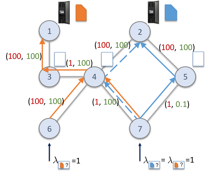
Appendix C Parameters for Example and Abilene

Parameter details are specified Fig. 7(a) and Fig. 7(b), for Ex2 and Abilene2, respectively. The differences between Ex1 and Ex2, Abilene1 and Abilene2 are different link capacities for some of edges. In particular, Ex1 and Ex2 differ on edge $(2,4)$ . This change is designed to make suboptimal algorithms infeasible in Ex1 and have high cost in Ex2. Abilene1 and Abilene2 differ on edge (Indianapolis,Chicago), (Indianapolis,Kansas City), and (Sunnyvale to Denver). The differences are designed again so that the first topology is infeasible and the second leads to high cost under suboptimal algorithms.