On low-depth algorithms for quantum phase estimation
Abstract
Quantum phase estimation is one of the critical building blocks of quantum computing. For early fault-tolerant quantum devices, it is desirable for a quantum phase estimation algorithm to (1) use a minimal number of ancilla qubits, (2) allow for inexact initial states with a significant mismatch, (3) achieve the Heisenberg limit for the total resource used, and (4) have a diminishing prefactor for the maximum circuit length when the overlap between the initial state and the target state approaches one. In this paper, we prove that an existing algorithm from quantum metrology can achieve the first three requirements. As a second contribution, we propose a modified version of the algorithm that also meets the fourth requirement, which makes it particularly attractive for early fault-tolerant quantum devices.
keywords
Quantum phase estimation, early fault-tolerant quantum devices.1 Introduction
Quantum phase estimation (QPE) is one of the most important building blocks of quantum computing. Consider a unitary matrix . Let be the orthogonal eigenstates of , and be the corresponding eigenvalues. In the QPE problem, given and an eigenstate, say , the goal is to estimate up to a certain accuracy. In a more general and practical setting, the initial quantum state provided for phase estimation is a linear combination of eigenstates, i.e., , where the coefficient for dominates.
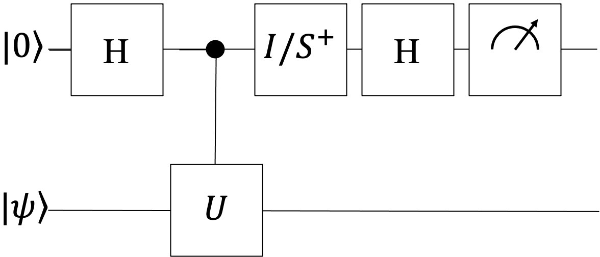
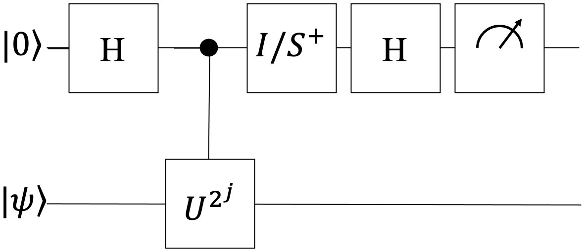
Due to the significance of QPE, many algorithms have been devised to address this problem. The well-known Hadamard test provides probably the simplest circuit (see Figure 1(a)) for this purpose, but it requires executions to reach a precision . Improving on the Hadamard test, Kitaev’s algorithm [13, 14] identifies the phase bit-by-bit by using quantum circuits with dyadic powers (see Figure 1(b)). It reduces the total complexity but is only applicable to exact eigenstates. The QPE algorithm based on quantum Fourier transform (QFT) [4] requires only a single run but a relatively large number of ancilla qubits. Many alternatives for QPE have been proposed in the literature [3, 9, 15, 22, 21, 7, 17, 18, 5, 28, 27, 26]. Among them, [28, 27] focus on the case of ground state energy estimation and a spectral gap is assumed. For a more comprehensive overview of the QPE algorithms, we refer to the detailed discussions in [5, 18, 20].
 |
 |
| (a) | (b) |
There are several key complexity metrics for evaluating the performance of the QPE algorithms. The first is the number of ancilla qubits required; the smaller, the better. The second one is the maximum runtime , measured by the maximum depth of any circuit used by the algorithm. The third one is the total runtime , equal to the sum of the circuit depths over all executions. It has been demonstrated (see [8, 30, 29] for example) that must follow the Heisenberg limit . The fourth one is the minimal overlap required between the initial state and the target state . A lower bound of this overlap is usually assumed because the problem of finding is otherwise shown to be difficult ([14, 11, 1]). Among these metrics, a small is particularly important for early fault-tolerant quantum devices since these devices typically have a small number of qubits and a relatively short coherence time. For the phase estimation problem, one can use similar ideas to the proof of lower bound in [10] to show that , which means when . A detailed proof is given in [25]. In conclusion, a near-optimal phase estimation algorithm should meet the following requirements:
- 1.
Use a small number of (even a single) ancilla qubits.
- 2.
Allow the initial state to be inexact.
- 3.
Achieve the Heisenberg-limited scaling .
- 4.
, and the prefactor can be arbitrarily small when approaches to the exact eigenstate . As we mentioned, this is particularly important for early fault-tolerant quantum devices.
Most of the proposed QPE algorithms fail to meet all four requirements. For example, the first requirement is violated by QPE algorithms using QFT. The Hadamard test and the original Kitaev algorithm violate the second requirement. The Hadamard test also violates the third requirement. It has been pointed out in [5] that the only algorithm proven to meet all four conditions is the recent optimization-based algorithm proposed in [5].
There have also been rapid developments of phase estimation in the related field of quantum metrology, such as [12, 2, 19, 23, 24]. For example, the robust phase estimation (RPE) algorithm in [12, 2, 24] halves the confidence interval of the phase iteratively to achieve the target accuracy. In this paper,
- •
we show that this RPE algorithm satisfies the first three requirements listed above as long as the initial overlap is above . This is an improvement over the threshold obtained in [5], and
- •
we propose a modified algorithm with a much shorter circuit length when the overlap approaches . The prefactor of can be as small as , which is better than the bound provided in [5].
The rest of the paper is organized as follows. Section 2 proves the correctness of RPE when the initial overlap is above . Section 3 presents the new algorithm that allows for shorter circuit length when the initial overlap approaches one.
2 Analysis of the existing algorithm
The angles and their computations are understood as modulo . The absolute value of an angle , denoted by , is defined to be the minimum distance to modulo , i.e., . For any quantum state , denote by the overlap between the given state and the eigenstate .
In the Hadamard test, the circuit in Figure 1(a) is used to estimate the real and imaginary parts of . In Kitaev’s algorithm, the circuits in Figure 1(b) are used to estimate the real and imaginary parts of for different values of . Algorithm 1 is a reformulation of the RPE outlined in [2], which uses the same primitives of the Kitaev’s algorithm and produces an approximation of with high probability. In the -th step, the Hadamard test is executed times to obtain an estimate of . Then is used to get a candidate set of new approximations of . The one closest to the previous approximation is chosen as the new approximation .
The following lemma is key to the analysis of Algorithm 1. Here, the constant serves as an upper bound for the noise in the initial state, i.e., .
Lemma 1.
Suppose the constant and let
| (1) |
If the quantum state satisfies and
| (2) |
then
| (3) |
where is the principal argument of .
Proof.
The following theorem is the main theoretical guarantee of Algorithm 1.
Theorem 2.
Suppose the constant and that the quantum state satisfies and
| (5) |
where is defined in (1). Then the output of Algorithm 1 satisfies
| (6) |
In addition, the maximal runtime and the total cost of Algorithm 1 are, respectively,
| (7) |
Proof.
First, we claim that under the circumstances of
| (8) |
. In fact, we can show
| (9) |
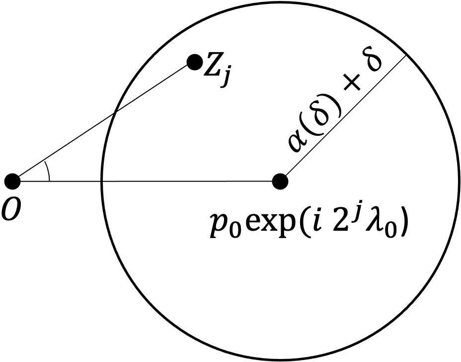
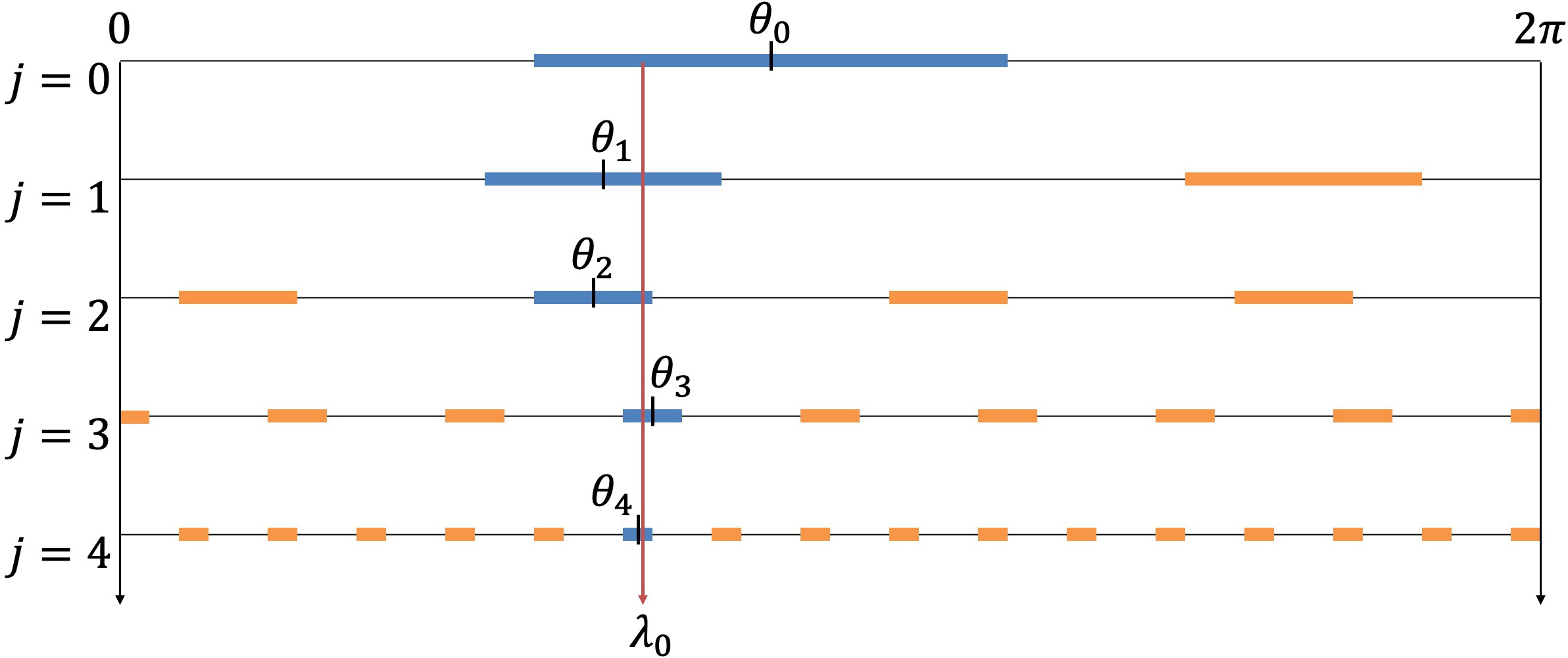
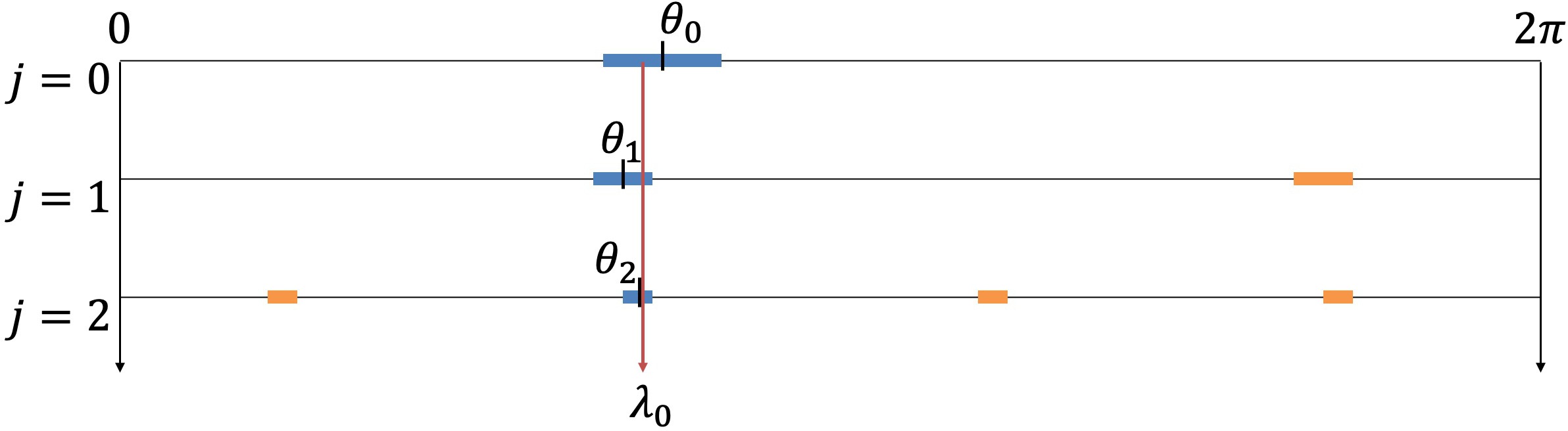
by induction. The case is a direct consequence of Lemma 1. Now if (9) holds for , then Lemma 1 states that is in one of the intervals for . Checking the length of the gaps between these intervals shows that only one such interval with can have a non-empty intersection with (see Figure 3). Recall that this is exactly the criteria for choosing . Hence .
It remains now to prove that (8) holds with a probability greater than . By Hoeffding’s inequality, using samples ensures that
| (10) |
for every . Therefore, we conclude that
| (11) |
∎
3 Low-depth circuit for large initial overlap
This section shows that the maximal runtime can be further reduced when the initial overlap is close to one (i.e., the upper bound of the noise in the initial state ). This is achieved via Algorithm 2.
In order to analyze the complexity of Algorithm 2, we need a generalization of Lemma 1 as provided below.
Lemma 3.
Suppose that and . Let
| (12) |
If the quantum state satisfies and an estimator satisfies
| (13) |
then
| (14) |
Proof.
Remark 4.
If we know a priori that the overlap between and is large, i.e., , we have . Thus, the constraint on enforced in Lemma 3 is in the regime of large overlap.
Here, we generalize the result presented in Theorem 2 and show that Algorithm 2 can give a further reduced . Notice that even though the assumption on still reads , Theorem 5 only provides substantial reduction on when is sufficiently small.
Theorem 5.
Assume that the quantum state satisfies , where . Suppose that , and that the parameter in Algorithm 2 is given by:
| (16) |
Then the output of Algorithm 2 satisfies
| (17) |
In addition, the maximal runtime and the total cost of Algorithm 2 are, respectively,
| (18) |
Proof.
Similar to Theorem 2, we first prove that under the circumstance of
| (19) |
. We proceed to show
| (20) |
by induction. The case is a direct corollary of Lemma 3. Now assume that (20) holds for . It is guaranteed by Lemma 3 that is in one of the intervals for . Since , the same argument as in Theorem 2 shows that at most one such interval with can have a non-empty intersection with (see Figure 4). Since this is the criteria for choosing in the algorithm, we have . Plugging in yields .
Now we show that (19) holds with a probability greater than . In fact, by Hoeffding’s inequality, with samples from the Hadamard test, one can ensure that
| (21) |
for every . Thus, with the union bound, one arrives at
| (22) |
∎
Remark 6.
It is worth noticing that when reducing to , will increase to . Therefore, a trade-off similar to [5] exists between and . In particular, by using a small prefactor in the large overlap regime, one reduces to (while increasing the total runtime to ). According to 4, Algorithm 2 reduces the maximal circuit length by a factor of , while the result presented in [5] only gives a factor of . After the initial submission of our manuscript, an extended version of QCELS is shown in [6] to achieve the factor with a more sophisticated analysis.
Remark 7.
The result in Algorithm 2 can be extended to the case with large relative overlap (Cf. [18, 5]) without increasing the depth of the quantum circuit. The filtering process and proof in [5] can be directly applied here. Briefly speaking, if one knows a priori that , then one only needs instead of . The idea is to replace , which is an estimator of , with an estimator of
Here is a matrix such that and is an approximation of the indicator up to precision , which is obtained by a truncation of the Fourier series of . The estimator of is then constructed with the results of Hadamard tests and the coefficients of the Fourier series.
| (a) | (b) |
4 Numerical simulation
In this section, we present the results of numerical simulations of our algorithms and compare our method to other phase estimation algorithms. The unitary operator we employ is defined as , where is a Hamiltonian and represents the operator -norm. The scaling factor in the exponential is used to ensure that the eigenvalues are all in , thereby eliminating any ambiguity arising from modulo .
Specifically, we employ the one-dimensional transverse field Ising model with sites and periodic boundary conditions as the Hamiltonian, which is given by
with parameters and . Here, and represent the Pauli matrices acting on the -th site.
In Figure 5, we present the performance of our RPE algorithm (Algorithm 1) and compare it to two other algorithms, namely the QCELS algorithm (the optimization-based method in [5]) and the textbook version QPE [4], with two different initial overlap. The parameters for QCELS are set identically to those in [5]. All data for these three methods are obtained by conducting ten random experiments and calculating the average error. As demonstrated in Figure 5(a), the error given by RPE and QCELS decreases when increasing with a linear trend for both and , and both RPE and QCELS provide a much smaller prefactor than textbook QPE. On the other hand, it is clear from Figure 5(b) that Algorithm 1 achieves a lower total cost compared to QCELS.
| (a) | (b) |
In the second numerical experiment, we consider the same unitary operator but assume that the initial overlap is sufficiently large, and we proceed to verify that Algorithm 2 can further reduce the prefactor in by lowering the value of in this regime. In particular, we assume that the initial overlap is . Then can be as small as according to Theorem 5. Figure 6 displays the results for Algorithm 2 with different values of , where the error is also averaged from random experiments. For the three different values , , and , the error shows a similar linear decreasing trend while the maximal runtime and the total runtime increase, which indicates that the difference only lies in the prefactor. Moreover, the prefactor of decreases as decreases, at the expense of an increase in , which verifies the conclusions of Theorem 5.
5 Conclusion and discussion
In this paper, we have demonstrated through theoretical analyses and numerical experiments that a simple RPE-type algorithm and its variant can be particularly suitable for the implementation of phase estimation on early fault-tolerant quantum computers since they satisfy the requirements (1), (2), (3) and (4). Compared with the previous work [5], our method is structurally simpler since no optimization procedure is needed. Our method also provides a more significant prefactor reduction while at the same time posing a looser requirement for the initial overlap.
For the theoretical results presented in this paper, a large probability statement is adopted. One can also easily extend the results to the other metrics, such as the mean squared error (MSE), where a different number of measurements can be used in each iteration to minimize the MSE.
The unitary is assumed to be a black-box unitary in the setting of this paper. When other powers of apart from are accessible, it is possible to relax further the requirement (see the follow-up work [16] for details). The fact that only needs to be smaller than an threshold makes the algorithm presented here specifically suitable for the case where the unitary comes from a simulation of a Hamiltonian of interest. In that case, the result shown here only requires an approximate simulation with precision for each time duration , thus making the algorithm particularly advantageous for the combination with Hamiltonian simulation algorithms.
References
- Aharonov and Naveh [2002] D. Aharonov and T. Naveh. Quantum NP-a survey. arXiv preprint quant-ph/0210077, 2002. doi: https://doi.org/10.48550/arXiv.quant-ph/0210077.
- Belliardo and Giovannetti [2020] F. Belliardo and V. Giovannetti. Achieving Heisenberg scaling with maximally entangled states: An analytic upper bound for the attainable root-mean-square error. Physical Review A, 102(4):042613, 2020. doi: https://doi.org/10.1103/PhysRevA.102.042613.
- Berry et al. [2015] D. W. Berry, A. M. Childs, R. Cleve, R. Kothari, and R. D. Somma. Simulating Hamiltonian dynamics with a truncated Taylor series. Physical review letters, 114(9):090502, 2015. doi: https://doi.org/10.1103/PhysRevLett.114.090502.
- Cleve et al. [1998] R. Cleve, A. Ekert, C. Macchiavello, and M. Mosca. Quantum algorithms revisited. Proceedings of the Royal Society of London. Series A: Mathematical, Physical and Engineering Sciences, 454(1969):339–354, 1998. doi: https://doi.org/10.1098/rspa.1998.0164.
- Ding and Lin [2023a] Z. Ding and L. Lin. Even shorter quantum circuit for phase estimation on early fault-tolerant quantum computers with applications to ground-state energy estimation. PRX Quantum, 4(2):020331, 2023a. doi: https://doi.org/10.1103/PRXQuantum.4.020331.
- Ding and Lin [2023b] Z. Ding and L. Lin. Simultaneous estimation of multiple eigenvalues with short-depth quantum circuit on early fault-tolerant quantum computers. Quantum, 7:1136, 2023b. doi: https://doi.org/10.22331/q-2023-10-11-1136.
- Dong et al. [2022] Y. Dong, L. Lin, and Y. Tong. Ground-state preparation and energy estimation on early fault-tolerant quantum computers via quantum eigenvalue transformation of unitary matrices. PRX Quantum, 3(4):040305, 2022. doi: https://doi.org/10.1103/PRXQuantum.3.040305.
- Giovannetti et al. [2006] V. Giovannetti, S. Lloyd, and L. Maccone. Quantum metrology. Physical review letters, 96(1):010401, 2006. doi: https://doi.org/10.1103/PhysRevLett.96.010401.
- Higgins et al. [2007] B. L. Higgins, D. W. Berry, S. D. Bartlett, H. M. Wiseman, and G. J. Pryde. Entanglement-free Heisenberg-limited phase estimation. Nature, 450(7168):393–396, 2007. doi: https://doi.org/10.1038/nature06257.
- Huang et al. [2023] H.-Y. Huang, Y. Tong, D. Fang, and Y. Su. Learning many-body hamiltonians with heisenberg-limited scaling. Physical Review Letters, 130(20):200403, 2023. doi: https://doi.org/10.1103/PhysRevLett.130.200403.
- Kempe et al. [2006] J. Kempe, A. Kitaev, and O. Regev. The complexity of the local Hamiltonian problem. Siam journal on computing, 35(5):1070–1097, 2006. doi: https://doi.org/10.1137/S0097539704445226.
- Kimmel et al. [2015] S. Kimmel, G. H. Low, and T. J. Yoder. Robust calibration of a universal single-qubit gate set via robust phase estimation. Physical Review A, 92(6):062315, 2015. doi: https://doi.org/10.1103/PhysRevA.92.062315.
- Kitaev [1995] A. Y. Kitaev. Quantum measurements and the abelian stabilizer problem. arXiv preprint quant-ph/9511026, 1995. doi: https://doi.org/10.48550/arXiv.quant-ph/9511026.
- Kitaev et al. [2002] A. Y. Kitaev, A. Shen, M. N. Vyalyi, and M. N. Vyalyi. Classical and quantum computation. American Mathematical Soc., 2002. doi: http://dx.doi.org/10.1090/gsm/047.
- Knill et al. [2007] E. Knill, G. Ortiz, and R. D. Somma. Optimal quantum measurements of expectation values of observables. Physical Review A, 75(1):012328, 2007. doi: https://doi.org/10.1103/PhysRevA.75.012328.
- Li et al. [2023] H. Li, H. Ni, and L. Ying. On low-depth quantum algorithms for robust multiple-phase estimation. arXiv preprint arXiv:2303.08099, 2023. doi: https://doi.org/10.48550/arXiv.2303.08099.
- Lin and Tong [2020] L. Lin and Y. Tong. Near-optimal ground state preparation. Quantum, 4:372, 2020. doi: https://doi.org/10.22331/q-2020-12-14-372.
- Lin and Tong [2022] L. Lin and Y. Tong. Heisenberg-limited ground-state energy estimation for early fault-tolerant quantum computers. PRX Quantum, 3(1):010318, 2022. doi: https://doi.org/10.1103/PRXQuantum.3.010318.
- Lumino et al. [2018] A. Lumino, E. Polino, A. S. Rab, G. Milani, N. Spagnolo, N. Wiebe, and F. Sciarrino. Experimental phase estimation enhanced by machine learning. Physical Review Applied, 10(4):044033, 2018. doi: https://doi.org/10.1103/PhysRevApplied.10.044033.
- Nielsen and Chuang [2000] M. A. Nielsen and I. L. Chuang. Quantum Computation and Quantum Information. Cambridge University Press, 2000. doi: http://dx.doi.org/10.1017/CBO9780511976667.
- O’Brien et al. [2019] T. E. O’Brien, B. Tarasinski, and B. M. Terhal. Quantum phase estimation of multiple eigenvalues for small-scale (noisy) experiments. New Journal of Physics, 21(2):023022, 2019. doi: 10.1088/1367-2630/aafb8e.
- Poulin and Wocjan [2009] D. Poulin and P. Wocjan. Sampling from the thermal quantum gibbs state and evaluating partition functions with a quantum computer. Physical review letters, 103(22):220502, 2009. doi: https://doi.org/10.1103/PhysRevLett.103.220502.
- Rudinger et al. [2017] K. Rudinger, S. Kimmel, D. Lobser, and P. Maunz. Experimental demonstration of a cheap and accurate phase estimation. Physical review letters, 118(19):190502, 2017. doi: https://doi.org/10.1103/PhysRevLett.118.190502.
- Russo et al. [2021] A. E. Russo, K. M. Rudinger, B. C. Morrison, and A. D. Baczewski. Evaluating energy differences on a quantum computer with robust phase estimation. Physical review letters, 126(21):210501, 2021. doi: https://doi.org/10.1103/PhysRevLett.126.210501.
- Tong [2021] Y. Tong. A tight query complexity lower bound for phase estimation under circuit depth constraint, 2021. URL https://math.berkeley.edu/˜yu_tong/lower_bound_low_depth_phase_est.pdf.
- Wan et al. [2022] K. Wan, M. Berta, and E. T. Campbell. Randomized quantum algorithm for statistical phase estimation. Physical Review Letters, 129(3):030503, 2022. doi: https://doi.org/10.1103/PhysRevLett.129.030503.
- Wang et al. [2022] G. Wang, D. Stilck-França, R. Zhang, S. Zhu, and P. D. Johnson. Quantum algorithm for ground state energy estimation using circuit depth with exponentially improved dependence on precision. arXiv preprint arXiv:2209.06811, 2022. doi: https://doi.org/10.48550/arXiv.2209.06811.
- Zhang et al. [2022] R. Zhang, G. Wang, and P. Johnson. Computing ground state properties with early fault-tolerant quantum computers. Quantum, 6:761, 2022. doi: https://doi.org/10.22331/q-2022-07-11-761.
- Zhou et al. [2018] S. Zhou, M. Zhang, J. Preskill, and L. Jiang. Achieving the Heisenberg limit in quantum metrology using quantum error correction. Nature communications, 9(1):78, 2018. doi: https://doi.org/10.1038/s41467-017-02510-3.
- Zwierz et al. [2010] M. Zwierz, C. A. Pérez-Delgado, and P. Kok. General optimality of the Heisenberg limit for quantum metrology. Physical review letters, 105(18):180402, 2010. doi: https://doi.org/10.1103/PhysRevLett.105.180402.