Contrast with Reconstruct: Contrastive 3D Representation Learning
Guided by Generative Pretraining

Zekun Qi Affiliation: Xi’an Jiaotong University Runpei Dong Affiliation: Xi’an Jiaotong University Guofan Fan Affiliation: Xi’an Jiaotong University Zheng Ge Affiliation: MEGVII Technology Xiangyu Zhang Affiliation: MEGVII Technology Kaisheng Ma Affiliation: Tsinghua University Correspondence to: kaisheng@mail.tsinghua.edu.cn Li Yi Affiliation: Tsinghua University Affiliation: Shanghai AI Laboratory Affiliation: Shanghai Qi Zhi Institute Correspondence to: ericyi@mail.tsinghua.edu.cn

Abstract

Mainstream 3D representation learning approaches are built upon contrastive or generative modeling pretext tasks, where great improvements in performance on various downstream tasks have been achieved. However, we find these two paradigms have different characteristics: (i) contrastive models are data-hungry that suffer from a representation over-fitting issue; (ii) generative models have a data filling issue that shows inferior data scaling capacity compared to contrastive models. This motivates us to learn 3D representations by sharing the merits of both paradigms, which is non-trivial due to the pattern difference between the two paradigms. In this paper, we propose Contrast with Reconstruct (ReCon) that unifies these two paradigms. ReCon is trained to learn from both generative modeling teachers and single/cross-modal contrastive teachers through ensemble distillation, where the generative student guides the contrastive student. An encoder-decoder style ReCon-block is proposed that transfers knowledge through cross attention with stop-gradient, which avoids pretraining over-fitting and pattern difference issues. ReCon achieves a new state-of-the-art in 3D representation learning, e.g., 91.26% accuracy on ScanObjectNN. Codes have been released at https://github.com/qizekun/ReCon.

Keywords:

Machine Learning, ICML, Representation Learning, GPT, Contrastive Learning, Generative Modeling, 3D Point Clouds

^†^†affiliationnotice: Equal contribution\icmlInternNotice

1 Introduction

Self-supervised representation learning (SSRL) has witnessed a booming era of foundational models (Bommasani et al. 2021), significant advancements are being made in natural language processing (NLP) (Radford et al. 2018; Devlin et al. 2019; Brown et al. 2020; Wei et al. 2022b; Ouyang et al. 2022), 2D machine vision (He et al. 2020; He et al. 2022), and both (vision-language, VL) (Radford et al. 2021; Rombach et al. 2022; Alayrac et al. 2022). While this great course toward foundational machine intelligence is trending, the success of these methods generally demands training on data of extreme size. However, compared to 2D vision and NLP, 3D vision is faced with a challenging data desert issue (Dong et al. 2023) due to collection difficulty.

Refer to caption — Figure 1: Data efficiency comparison and attention distance visualization. (a) Fine-tuning overall accuracy on ScanObjectNN PB_T50_RS with models pretrained with different methods on ShapeNet of different data ratios. (b) Averaged attention distance of models pretrained on ShapeNet with generative masked point modeling (MPM) (Pang et al. 2022) and cross-modal contrastive (CMC) modeling (Radford et al. 2021) (texts, images, and point clouds are used), respectively. SUP: supervised classification pretraining on ShapeNet. SMC: single-modal contrastive pretraining (Khosla et al. 2020). ReCon-SMC and ReCon-CMC represent our proposed ReCon with single-modal and cross-modal contrastive modeling variants, respectively. MPM+SMC and MPM+CMC represent vanilla multi-task learning.

Though under this low-data regime, numerous 3D SSRL methods have been developed, which can be grouped into two categories, i.e., contrastive (single/cross-modal) (Xie et al. 2020; Zhang et al. 2021; Chen et al. 2022; Liu et al. 2021a; Afham et al. 2022) and generative (reconstruct/predict) (Wang et al. 2021; Yu et al. 2022b; Pang et al. 2022) methods. However, we investigate the pretraining efficiency of the two paradigms by scaling the pretraining data of ShapeNet ranging from 1% to 100%, and we find that these two paradigms have their issues (see Fig. 1(a)):

•

Representation over-fitting (contrastive). Contrastive models fail to bring generalization when the pretraining data is lacking ( $<90\%$ ), while generative models bring significant improvements with only $\sim 25\%$ data. It shows that contrastive models can easily find shortcuts with trivial representations that over-fit the limited data (He et al. 2020), and generative models are less data-hungry that learn decent initialization with very few data (Kong & Zhang 2023).
•

Data filling (generative). Contrastive models present a better potential with scaled-up data, while generative models only provide a little improvement. It shows that contrastive learning may bring superior data-scaling capacity when the pretraining data is sufficient. This is observed in 2D where contrastive models surpass generative models (Dong et al. 2022) that have less scaling capability (Xie et al. 2022b).

These observations motivate the design that shares both merits without mentioned issues. However, as shown in Fig. 1(a), simply combining these two paradigms as multi-task learning leads to unsatisfactory results – lower than the generative model baseline and the representation over-fitting issue remains. To understand why, we visualize the averaged attention distance¹¹ 1 The attention distance are conducted by averaging per attention head for each layer following Dosovitskiy et al. 2021, which reveals the relative receptive field of the learned attention. of the contrastive and generative models in Fig. 1(b). A pattern difference issue is observed that the attention of contrastive models is mainly paid to a global field, while generative models have an appetite for focused local attention, which is consistent with the observations by Xie et al. 2022a in 2D. We conject that this pattern difference issue causes a task conflict in the naive multi-task representation learning setting, indicating it is non-trivial to combine the merits of contrastive and generative modeling.

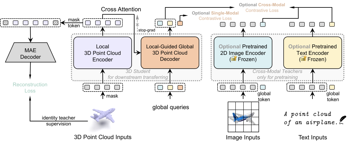
To address the above-mentioned issues, we propose Contrast with Reconstruct (ReCon) that trains generative modeling as guidance for contrastive learning while sharing both merits. As shown in Fig. 2, from the perspective of knowledge distillation (Sec. 3.1), contrastive and generative methods can be viewed as vanilla student-teacher paradigms (Fig. 2(a-b)). In contrast, our ReCon unifies the two paradigms as ensemble distillation from multi-teachers, while the generative student is also a “teacher” which guides the contrastive learning (student-teacher knowledge distillation with student-student assistance).

In particular, inspired by Vaswani et al. 2017, a novel encoder-decoder style ReCon-block is proposed where cross attention with stop-gradient is used to transfer guidance from reconstruction to contrastive modeling. In this fashion, the knowledge from multi-teachers is disentangled and reinforced, which addresses the representation over-fitting issue and avoids the learned pattern difference. Further, our ReCon utilizes single-modal or cross-modal contrastive learning of 3D point clouds, 2D RGB images, and languages that significantly enlarge the pretraining data diversity and capacity. Meanwhile, the data-filling issue of the generative student is alleviated due to the promising scaling capacity of the contrastive student. Fig. 1(b) shows that our ReCon learns 3D representations with high generalization capacity. By transferring the learned representations to various benchmarks, a new state-of-the-art in self-supervised 3D learning is achieved. For example, an average improvement of +9.2% and +2.9% accuracy are achieved on ScanObjectNN and ModelNet40, respectively. These results show that ReCon learns foundational geometric understanding, and this simple and general framework successfully unifies contrastive and generative modeling.

2 Related Works

Contrastive Representation Learning is one of the mainstream self-supervised learning paradigms (Hadsell et al. 2006), which learns potential semantics from constructed invariance or equivaiance (Dangovski et al. 2022). Generally, Instance Discrimination (Wu et al. 2018) is widely adopted to align and distinguish representations of views with the same high-level semantics or not. The views could be constructed by augmentations to single-modal (Chen et al. 2020; He et al. 2020; Chen et al. 2021) or multi-modal data (Radford et al. 2021; Li et al. 2022a). Most works use global features for processing. For example, SimCLR (Chen et al. 2020) uses samples with different augmentation policies to construct positive and negative pairs. CLIP (Radford et al. 2021) proposes a two-tower network that aligns the global representation of languages and images. Driven by InforMAX principle (Hjelm et al. 2019), they generally use InfoNCE (van den Oord et al. 2018) as the loss function to maximize mutual information. In 3D, PointContrast (Xie et al. 2020) proposes geometric augmentation to generate positive and negative pairs. CrossPoint (Afham et al. 2022) uses both inter and intra-modal contrastive learning. PointCLIP (Zhang et al. 2022c) realizes image-point alignment by projecting point clouds to 2D depth images. In this work, we focus on single/cross-modal contrastive learning by discriminative contrast (Khosla et al. 2020) or global feature alignment like Radford et al. 2021, which is guided by masked generative modeling.

Generative Masked Representation Learning has emerged as another paradigm of self-supervised learning from NLP (Devlin et al. 2019) to Vision (He et al. 2022). It requires the models to learn structured knowledge by reconstructing masked input data, which encourages the association of different local patches. In NLP, it has been a dominant approach to probing knowledge by recovering or predicting words in sentences (Devlin et al. 2019; Brown et al. 2020). With the rapid development of Transformers in vision (Dosovitskiy et al. 2021; Liu et al. 2021b), abundant works have been proposed to realize mask image modeling (MIM). He et al. 2022 propose masked autoencoder (MAE) to reconstruct RGB pixels. Bao et al. 2022 reconstructs the VQVAE (Ramesh et al. 2021) codebook with encoded semantics. Some works propose to reconstruct online teacher tokens (Zhou et al. 2022) or HOG features (Wei et al. 2022a). In 3D, PointMAE (Pang et al. 2022) extends MAE (He et al. 2022) by reconstructing masked point clouds. PointM2AE (Zhang et al. 2022b) uses a hierarchical Transformer and designs the corresponding masking strategy. MaskPoint (Liu et al. 2022) proposes to add some noise points and classify whether they belong to masking tokens. Recently, ACT (Dong et al. 2023) uses a cross-modal autoencoder as the reconstruction target to acquire dark knowledge from other modalities.

3 ReCon: Contrast with Reconstruct

Figure 3: Illustration of the proposed ReCon-block for pretraining. The local reconstruction task is used to train the encoder, while the global contrastive task is used to train the decoder guided by reconstruction-oriented embeddings with cross attention (CA). Stop-gradient (stop-grad) is applied to every CA connection to avoid misleading gradient flow from global to local.

We begin with a review in a unified view of knowledge distillation for the two mainstream representation learning methods: masked generative modeling and contrastive modeling. We then introduce ReCon that unifies these two representation learning methods by reconstruction-guided contrastive learning using an encoder-decoder style ReCon-block based architecture, where the overall representation learning is formulated as distillation with both teachers with student-student assistance.

3.1 Knowledge Distillation: A Unified View of Generative and Contrastive Learning

Contrastive Modeling

The key insight of contrastive learning lies in invariance learning (Kosmann-Schwarzbach 2011; He et al. 2020; Kong & Zhang 2023), where the abstraction of semantics is generally invariant or equivariant (Dangovski et al. 2022) to multiple transformed views like augmentations (Chen et al. 2020) or modalities (Tian et al. 2020a). From the perspective of knowledge distillation (Hinton et al. 2015), it can be viewed as a student network learning the invariance knowledge transferred from the encoded views of the teacher. Formally, given input data $x\sim\mathcal{D}$ with distribution $\mathcal{D}$ , the student network is $\mathcal{F}^{{S}}_{\theta}(\cdot)$ with parameters $\theta$ and $\mathcal{F}^{{T}}_{\phi}(\cdot)$ is the teacher network with parameters $\phi$ . The optimization target can be written:

	$\displaystyle\mathop{\min}\limits_{\theta}\mathop{\mathbb{E}}\limits_{\mathop{x\sim\mathcal{D},}\limits_{\{\mathcal{T}_{i},\mathcal{T}_{j}\}\in\mathcal{T}}}$	$\displaystyle{\displaystyle\mathcal{L}}^{\text{CON}}_{\mathbb{C}}(z_{i},z_{j}),$		(1)
		$\displaystyle z_{i}=\mathcal{F}^{{S}}_{\theta}\big(\mathcal{T}_{i}(x)\big),z_{j}=\mathcal{F}^{{T}}_{\phi}\big(\mathcal{T}_{j}(x)\big),$		(1)

where

•

The teacher parameters $\phi$ can be the same as $\theta$ with (Chen & He 2021) or without (Chen et al. 2020) stop-gradient, $\phi$ can also be the momentum counterpart updated as $\phi\leftarrow m\phi+(1-m)\theta$ where $m\in(0,1]$ is the momentum coefficient (He et al. 2020; Chen et al. 2021). For multi-modal inputs²² 2 Note that there are some methods (Tian et al. 2020a; Radford et al. 2021) that optimizes both $\theta$ and $\phi$ ., $\phi$ can be different from $\theta$ that encodes views from other modalities (Tian et al. 2020a; Radford et al. 2021; Jing et al. 2021).
•

$\{\mathcal{T}_{i}(\cdot),\mathcal{T}_{j}(\cdot)\}\in\mathcal{T}$ are two transformations of the input data that belongs to constructed transformation pairs $\mathcal{T}$ , where $\mathcal{T}_{j}(\cdot)$ constructs the positive or negative³³ 3 For methods use positive samples only (Grill et al. 2020; Chen & He 2021), $\mathcal{T}_{j}(\cdot)$ only generates positive views. invariance targets, respectively. In general, this transformation generates copied views by data augmentations (Caron et al. 2021; Wang & Qi 2021), we extend it to multi-modal inputs where the transformation becomes generating views from different modalities that share the same high-order concept (Radford et al. 2021; Liu et al. 2021a).
•

${\mathcal{L}}^{\text{CON}}_{\mathbb{C}}(\cdot,\cdot)$ is the distance function defined in some metric space $\mathbb{C}$ . To avoid representation collapsing (He et al. 2020), InfoMax-Principle (Hjelm et al. 2019; Bachman et al. 2019) based metrics like MINE (Belghazi et al. 2018), InfoNCE (van den Oord et al. 2018) are often used (He et al. 2020; Tian et al. 2020c; Zhang et al. 2022a). For methods using positive-only transformations, the metric function can be feature correlation measurement (Zbontar et al. 2021), $\ell_{2}$ distance (Ermolov et al. 2021), or cosine similarity (Grill et al. 2020; Chen & He 2021).

Generative Masked Modeling

Similarly, given input data $x\sim\mathcal{D}$ with distribution $\mathcal{D}$ , the student network as $\mathcal{F}^{{S}}_{\theta}(\cdot)$ with parameters $\theta$ and $\mathcal{F}^{{T}}_{\phi}(\cdot)$ as the teacher network⁴⁴ 4 Note that for methods like MAE (He et al. 2022; Pang et al. 2022), the teacher network is an identity mapping with no parameters, and therefore $\phi$ is an empty set, see Dong et al. 2023. with parameters $\phi$ . generative masked modeling can be formulated as follows:

	$\displaystyle\mathop{\min}\limits_{\theta}\mathop{\mathbb{E}}\limits_{\mathop{x\sim\mathcal{D},}\limits_{\{\mathcal{M}_{i},\widetilde{\mathcal{M}}_{i}\}\in\mathcal{M}}}$	$\displaystyle{\displaystyle\mathcal{L}}^{\text{REC}}_{\mathbb{D}}(z_{i},z_{j}),$		(2)
		$\displaystyle z_{i}=\mathcal{F}^{{S}}_{\theta}\big(\mathcal{M}_{i}(x)\big),z_{j}=\mathcal{F}^{{T}}_{\phi}\big(\widetilde{\mathcal{M}}_{i}(x)\big),$		(2)

where

•

${\mathcal{L}}^{\text{REC}}_{\mathbb{D}}$ is a distance function defined in some metric space $\mathbb{D}$ . It can be $\ell_{2}$ distance (He et al. 2022), cross-entropy (Devlin et al. 2019; Bao et al. 2022), or Chamfer-Distance (Fan et al. 2017; Pang et al. 2022).
•

$\{\mathcal{M}_{i},\widetilde{\mathcal{M}}_{i}\}\in\mathcal{M}$ are the masking corruptions where $\mathcal{M}_{i}(\cdot)$ samples a subset of the input tokens and performs masking (Devlin et al. 2019), and $\widetilde{\mathcal{M}}_{i}(\cdot)$ correspondingly samples the subset while without masking.

Table 1: Classification results on the ScanObjectNN and ModelNet40 datasets. The inference model parameters #P (M), FLOPS #F (G), and overall accuracy (%) are reported. The dagger (^†) denotes that the model was reproduced using our proposed

\bullet

ReCon-block and the fine-tuning techniques used in ReCon. We compare with methods using the

\mathbf{\circ}

hierarchical Transformer architectures (e.g., Point-M2AE (Zhang et al. 2022b)),

\bullet

plain Transformer architectures, and

\mathbf{\circ}

dedicated architectures for 3D understanding. PT: pretrained teacher is used, MD: multi-modal data is used. Single-Modal means that only point clouds are used as pre-training data.

Method	#P	#F	PT	MD	ScanObjectNN			ModelNet40
Method	#P	#F	PT	MD	OBJ_BG	OBJ_ONLY	PB_T50_RS	1k P	8k P
Supervised Learning Only
$\mathbf{\circ}$ PointNet (Qi et al. 2017a)	3.5	0.5	$\times$	$\times$	73.3	79.2	68.0	89.2	90.8
$\mathbf{\circ}$ PointNet++ (Qi et al. 2017b)	1.5	1.7	$\times$	$\times$	82.3	84.3	77.9	90.7	91.9
$\mathbf{\circ}$ DGCNN (Wang et al. 2019)	1.8	2.4	$\times$	$\times$	82.8	86.2	78.1	92.9	-
$\mathbf{\circ}$ PointCNN (Li et al. 2018)	0.6	-	$\times$	$\times$	86.1	85.5	78.5	92.2	-
$\mathbf{\circ}$ SimpleView (Goyal et al. 2021)	-	-	$\times$	$\times$	-	-	80.5 $\pm$ 0.3	93.9	-
$\mathbf{\circ}$ MVTN (Hamdi et al. 2021)	11.2	43.7	$\times$	$\times$	92.6	92.3	82.8	93.8	-
$\mathbf{\circ}$ PCT (Guo et al. 2021)	2.88	2.3	$\times$	$\times$	-	-	-	93.2	-
$\mathbf{\circ}$ PointMLP (Ma et al. 2022)	12.6	31.4	$\times$	$\times$	-	-	85.4 $\pm$ 0.3	94.5	-
$\mathbf{\circ}$ PointNeXt (Qian et al. 2022)	1.4	3.6	$\times$	$\times$	-	-	87.7 $\pm$ 0.4	94.0	-
$\mathbf{\circ}$ P2P-HorNet (Wang et al. 2022)	-	34.6	$\checkmark$	$\checkmark$	-	-	89.3	94.0	-
with Single-Modal Self-Supervised Representation Learning (Full)
$\bullet$ Transformer (Vaswani et al. 2017)	22.1	4.8	$\times$	$\times$	83.04	84.06	79.11	91.4	91.8
$\bullet$ Transformer^† (Vaswani et al. 2017)	43.6	5.3	$\times$	$\times$	84.90	86.12	81.64	91.6	92.0
$\bullet$ Point-BERT (Yu et al. 2022b)	22.1	4.8	$\times$	$\times$	87.43	88.12	83.07	93.2	93.8
$\bullet$ Point-MAE (Pang et al. 2022)	22.1	4.8	$\times$	$\times$	90.02	88.29	85.18	93.8	94.0
$\mathbf{\circ}$ Point-M2AE (Zhang et al. 2022b)	15.3	3.6	$\times$	$\times$	91.22	88.81	86.43	94.0	-
$\bullet$ Point-MAE^† (Pang et al. 2022)	43.6	5.3	$\times$	$\times$	92.60	91.91	88.42	93.8	94.0
$\bullet$ ReCon w/o vot.	43.6	5.3	$\times$	$\times$	94.15	93.12	89.73	93.6	93.8
$\bullet$ ReCon w/ vot.	43.6	5.3	$\times$	$\times$	94.49	93.29	90.35	93.9	94.2
with Cross-Modal Self-Supervised Representation Learning (Full)
$\bullet$ ACT (Dong et al. 2023)	22.1	4.8	$\checkmark$	$\times$	93.29	91.91	88.21	93.7	94.0
$\bullet$ ReCon-Tiny w/o vot.	11.4	2.4	$\checkmark$	$\checkmark$	93.80	92.94	89.10	93.3	93.6
$\bullet$ ReCon-Small w/o vot.	19.0	3.2	$\checkmark$	$\checkmark$	94.15	93.12	89.52	93.5	93.8
$\bullet$ ReCon w/o vot.	43.6	5.3	$\times$	$\checkmark$	94.66	93.29	90.32	94.0	94.2
$\bullet$ ReCon w/o vot.	43.6	5.3	$\checkmark$	$\checkmark$	95.18	93.63	90.63	94.1	94.3
$\bullet$ ReCon w/ vot.	43.6	5.3	$\checkmark$	$\checkmark$	95.35	93.80	91.26	94.5	94.7
with Self-Supervised Representation Learning (Mlp-Linear)
$\bullet$ Point-MAE^† (Pang et al. 2022)	43.6	5.3	$\times$	$\times$	82.77 $\pm$ 0.30	83.23 $\pm$ 0.16	74.13 $\pm$ 0.21	90.22 $\pm$ 0.09	90.73 $\pm$ 0.09
$\bullet$ ACT (Dong et al. 2023)	22.1	4.8	$\checkmark$	$\times$	85.20 $\pm$ 0.83	85.84 $\pm$ 0.15	76.31 $\pm$ 0.26	91.36 $\pm$ 0.17	91.75 $\pm$ 0.18
$\bullet$ ReCon w/o vot.	43.6	5.3	$\checkmark$	$\checkmark$	89.50 $\pm$ 0.20	89.72 $\pm$ 0.17	81.36 $\pm$ 0.14	92.47 $\pm$ 0.22	92.68 $\pm$ 0.07
with Self-Supervised Representation Learning (Mlp-3)
$\bullet$ Point-MAE^† (Pang et al. 2022)	43.6	5.3	$\times$	$\times$	85.78 $\pm$ 0.31	85.51 $\pm$ 0.16	80.38 $\pm$ 0.21	91.25 $\pm$ 0.24	91.68 $\pm$ 0.19
$\bullet$ ACT (Dong et al. 2023)	22.1	4.8	$\checkmark$	$\times$	87.14 $\pm$ 0.22	87.90 $\pm$ 0.40	81.52 $\pm$ 0.19	92.69 $\pm$ 0.18	92.95 $\pm$ 0.10
$\bullet$ ReCon w/o vot.	43.6	5.3	$\checkmark$	$\checkmark$	90.62 $\pm$ 0.22	90.71 $\pm$ 0.30	83.80 $\pm$ 0.42	93.00 $\pm$ 0.10	93.39 $\pm$ 0.05

Ensemble Representation Distillation Ensemble distillation⁵⁵ 5 Term taken from Tian et al. 2020b. is known to be more informative and instructive (Tian et al. 2020b; Park & Kwak 2020; Xiang et al. 2020; Wang & Yoon 2022), which encourages the student network to learn ensembled and disentangled knowledge representation. We motivate our method as an ensembled knowledge distillation of Eq. (1) and Eq. (2), where the student is trained with merits from both contrastive and generative aspects. The overall loss $\mathcal{L}^{\text{{ReCon}}}$ is defined as follows:

\mathcal{L}^{\text{{ReCon}}}=\mathcal{L}^{\text{REC}}+\mathcal{L}^{\text{CON}}.

(3)

3.2 Reconstruction Guided Contrastive Learning

Network Architecture As discussed in Sec. 1, since the two distillation result in different learning patterns, it is non-trivial to learn from both targets jointly. To tackle this issue, we propose contrast with reconstruct (ReCon). The reconstruction-oriented representations that focus on local patterns are used as semantic guidance for global contrastive learning. Inspired by the Transformer encoder-decoder architecture (Vaswani et al. 2017), we conduct dense masked modeling with an encoder, which produces features to guide global contrastive learning through a sparse query-based decoder. The encoder and decoder share the same Transformer architecture, and they are layer-wisely associated with cross attention (CA). Due to limited 3D data, the contrastive model can easily learn trivial representations as shortcuts, and this could lead to noisy training signals, which may harm generative student learning. Hence, to avoid the task conflicts between these two students, we use stop-gradient for every CA connection to cut the misleading training signal from global contrast to local reconstruction. We call the proposed network architecture ReCon-block, which is illustrated in Fig. 3. In this fashion, the ensemble “student-teacher” distillation from multi-teacher is learned jointly with “student-student” assistance where the contrastive student is guided by the generative “teacher”. As a result, the contrastive student is trained with a good data scaling capacity without the risk of representation over-fitting, and the pattern difference issue is avoided with no task conflicts.

Table 2: Few-shot classification results on ModelNet40. ^† represent results of our proposed

\bullet

ReCon-block built backbone architecture. Overall accuracy (%) without voting is reported.

with Self-Supervised Representation Learning (Full)
Method	5-way		10-way
Method	10-shot	20-shot	10-shot	20-shot
$\mathbf{\circ}$ DGCNN	31.6 $\pm$ 2.8	40.8 $\pm$ 4.6	19.9 $\pm$ 2.1	16.9 $\pm$ 1.5
$\mathbf{\circ}$ OcCo	90.6 $\pm$ 2.8	92.5 $\pm$ 1.9	82.9 $\pm$ 1.3	86.5 $\pm$ 2.2
$\bullet$ Transformer	87.8 $\pm$ 5.2	93.3 $\pm$ 4.3	84.6 $\pm$ 5.5	89.4 $\pm$ 6.3
$\bullet$ Transformer^†	90.2 $\pm$ 5.9	94.3 $\pm$ 4.4	85.2 $\pm$ 5.9	89.9 $\pm$ 6.1
$\mathbf{\circ}$ OcCo	94.0 $\pm$ 3.6	95.9 $\pm$ 2.3	89.4 $\pm$ 5.1	92.4 $\pm$ 4.6
$\bullet$ Point-BERT	94.6 $\pm$ 3.1	96.3 $\pm$ 2.7	91.0 $\pm$ 5.4	92.7 $\pm$ 5.1
$\bullet$ MaskPoint	95.0 $\pm$ 3.7	97.2 $\pm$ 1.7	91.4 $\pm$ 4.0	93.4 $\pm$ 3.5
$\bullet$ Point-MAE	96.3 $\pm$ 2.5	97.8 $\pm$ 1.8	92.6 $\pm$ 4.1	95.0 $\pm$ 3.0
$\mathbf{\circ}$ Point-M2AE	96.8 $\pm$ 1.8	98.3 $\pm$ 1.4	92.3 $\pm$ 4.5	95.0 $\pm$ 3.0
$\bullet$ Point-MAE^†	96.4 $\pm$ 2.8	97.8 $\pm$ 2.0	92.5 $\pm$ 4.4	95.2 $\pm$ 3.9
$\bullet$ ACT	96.8 $\pm$ 2.3	98.0 $\pm$ 1.4	93.3 $\pm$ 4.0	95.6 $\pm$ 2.8
$\bullet$ ReCon	97.3 $\pm$ 1.9	98.9 $\pm$ 1.2	93.3 $\pm$ 3.9	95.8 $\pm$ 3.0
with Self-Supervised Representation Learning (Mlp-Linear)
$\bullet$ Point-MAE^†	91.1 $\pm$ 5.6	91.7 $\pm$ 4.0	83.5 $\pm$ 6.1	89.7 $\pm$ 4.1
$\bullet$ ACT	91.8 $\pm$ 4.7	93.1 $\pm$ 4.2	84.5 $\pm$ 6.4	90.7 $\pm$ 4.3
$\bullet$ ReCon	96.9 $\pm$ 2.6	98.2 $\pm$ 1.4	93.6 $\pm$ 4.7	95.4 $\pm$ 2.6
with Self-Supervised Representation Learning (Mlp- $3$ )
$\bullet$ Point-MAE^†	95.0 $\pm$ 2.8	96.7 $\pm$ 2.4	90.6 $\pm$ 4.7	93.8 $\pm$ 5.0
$\bullet$ ACT	95.9 $\pm$ 2.2	97.7 $\pm$ 1.8	92.4 $\pm$ 5.0	94.7 $\pm$ 3.9
$\bullet$ ReCon	97.4 $\pm$ 2.2	98.5 $\pm$ 1.4	93.6 $\pm$ 4.7	95.7 $\pm$ 2.7

Implementation We use the standard plain Transformer (Vaswani et al. 2017) built with 12 ReCon-blocks with dimension 384 and a lightweight PointNet patch embedding (Qi et al. 2017a; Qi et al. 2017b; Yu et al. 2022b) as the 3D representation learner. ShapeNet (Chang et al. 2015) is used to pretrain ReCon, which contains $\sim$ 51K unique 3D CAD models covering 55 object categories. We follow Khosla et al. 2020 for single-modal contrastive modeling. For cross-modal setting, we utilize point clouds, RGB images, and free-form languages, where the limited 3D data is enlarged with rich texture and semantic knowledge within images and languages (Afham et al. 2022; Dong et al. 2023). We obtain RGB images by rendering from 3D meshes and language descriptions by concatenating text prompts with category descriptions. We use by default an ImageNet (Deng et al. 2009) pretrained Vision Transformer (ViT-B) (Dosovitskiy et al. 2021) as the image view teacher, and we use the text encoder from CLIP (Radford et al. 2021) as the text view teacher. The image and text teacher encoders are frozen during pretraining, and Smooth $\ell_{1}$ -based positive-only distillation (Chen & He 2021; Ermolov et al. 2021) is used. The masked generative modeling follows Pang et al. 2022, where the reconstruction metric is $\ell_{2}$ Chamfer-Distance (Fan et al. 2017). Fig. 4 shows an overall illustration and more details can be found in Appendix B.

4 Experiments

4.1 Transfer Learning on Downstream Tasks

Transfer Protocol

We use the same classification heads and transfer learning protocols following Dong et al. 2023: Full, Mlp-Linear, and Mlp- $3$ .

3D Real-World Object Recognition ScanObjectNN (Uy et al. 2019) is one of the most challenging 3D datasets, which covers $\sim$ 15K real-world objects from 15 categories. For a fair comparison, we report the results with and without the voting strategy (Liu et al. 2019) separately. Note that we only use simple Rotation as data augmentation in training following Dong et al. 2023. We report single-modal (ReCon-SMC) and cross-modal (ReCon-CMC, default if not otherwise specified) results on three model variants (see Appendix B.) The results are shown in Table 1, it is observed that: (i) With a comparable GFLOPS, the performance of our ReCon-block (from scratch) is improved by 2.5% compared with that of standard Transformer under Full tuning protocol. Further, after the pre-training of reconstruction guided contrastive learning, ReCon gains a significant improvement of +11.3% accuracy averaged on the three variant ScanObjectNN benchmarks. (ii) Compared to other self-supervised learning (SSL) methods, our ReCon achieves the best generalization across both single-modal and cross-modal on all transferring protocols. e.g., ReCon outperforms Point-MAE by +5.6% on three ScanObjectNN variants. (iii) Compared with any supervised or self-supervised method, our ReCon achieves a new state-of-the-art that outperforms existing methods by a large margin.

Figure 5: Ablation study of masking ratio, decoder depth, and the 2D teacher encoder choice used during ReCon pretraining. The masking ratio and decoder depth represent the ablation for the generative masked modeling stream, and the 2D teachers are used for contrastive cross-modal learning.

3D Synthetic Object Recognition ModelNet (Wu et al. 2015) is one of the most classical datasets for synthetic 3D object recognition. It contains $\sim$ 12K meshed 3D CAD objects of 40 (ModelNet40) or 10 (ModelNet10) categories. We conduct the evaluation on the ModelNet40 dataset, including fine-tuning and few-shot learning. We use Scale&Translate as data augmentation in training following Qi et al. 2017a; Qi et al. 2017b. The results are shown in Table 1 and Table 2, respectively. It can be observed that our ReCon achieves 94.7% classification accuracy of ModelNet40 under Full protocol, improved by 2.7% compared with the Transformer baseline. In the few-shot task, our ReCon has also achieved the best performance under all protocols, especially under the Mlp- $3$ and Mlp-Linear protocols.

Table 3: Zero-shot 3D object classification domain transfer on ModelNet40 (MN-40) and ModelNet10 (MN-10). Top-1 accuracy (%) is reported. Ensemb. denotes whether to use the ensemble strategy with multiple text inputs.

Method	Backbone	Ensemb.	MN-10	MN-40
$\mathbf{\circ}$ PointCLIP (Zhang et al. 2022c)	ResNet-50	$\times$	30.2	20.2
$\bullet$ CLIP2Point (Huang et al. 2022)	Transformer	$\checkmark$	66.6	49.4
$\bullet$ ReCon	Transformer	$\times$	74.2	60.6
$\bullet$ ReCon	Transformer	$\checkmark$	75.6	61.7

3D Zero-Shot Recognition Similar to CLIP (Radford et al. 2021), our model aligns the feature space of languages and other modalities. Therefore, our model has a strong zero-shot capability. We use ModelNet (Wu et al. 2015) dataset to conduct zero-shot evaluation, including ModelNet10 and ModelNet40. The results are shown in Table 3. Following PointCLIP (Zhang et al. 2022c), We use prompt templates with the category label to generate text features. From Table 3, it can be seen that our ReCon surpasses all the zero-shot methods with CNN-based or Transformer-based backbones. Further, by using ensemble methods such as multi-prompt templates (Huang et al. 2022), our ReCon achieves a Top-1 accuracy of 61.7% on ModelNet40, which significantly outperforms PointCLIP and CLIP2Point by 41.5% and 12.3%, respectively.

Table 4: Ablation study on pretraining targets. Overall accuracy (%) without voting is reported.

Reconstruction	Contrastive			ScanObjectNN
Reconstruction	text	image	self	ScanObjectNN
$\times$	$\checkmark$	$\times$	$\times$	85.60
$\times$	$\times$	$\checkmark$	$\times$	86.02
$\times$	$\times$	$\times$	$\checkmark$	85.57
$\times$	$\checkmark$	$\checkmark$	$\times$	86.49
$\checkmark$	$\times$	$\times$	$\times$	88.42
$\checkmark$	$\checkmark$	$\times$	$\times$	89.77
$\checkmark$	$\times$	$\checkmark$	$\times$	90.18
$\checkmark$	$\times$	$\times$	$\checkmark$	89.50
$\checkmark$	$\checkmark$	$\checkmark$	$\times$	90.63
$\checkmark$	$\checkmark$	$\checkmark$	$\checkmark$	89.98

4.2 Ablation Study

Hyper Parameter In Fig. 5, We show the ablation study on masking ratio, decoder depth, and the selection of the 2D image teacher during ReCon pretraining. It can be observed that the optimal masking ratio and decoder depth is consistent with Point-MAE (Pang et al. 2022), indicating that the pretraining model, which is friendly to downstream tasks, is also helpful for the guidance of contrastive learning. The results also show that ViT (Dosovitskiy et al. 2021), as a 2D teacher, is superior to CLIP (Radford et al. 2021), Swin-Transformer (Swin) (Liu et al. 2021b), ResNet (He et al. 2016) and BEiT (Bao et al. 2022). In addition, we find that CLIP, which is already aligned with languages, brings inferior performance to ViT. This may be due to the reduction of diversity caused by the high similarity of features from the pre-aligned text teacher, which can be considered degenerating to only a single vision-language pretrained teacher.

Pretraining Targets To analyze the importance of the pretraining targets and verify the effect of reconstruction-guided contrastive modeling, we conduct an ablation study on the pretraining target. The results are shown in Table 4. It can be seen that: (i) When reconstruction guidance is not used, the performance of the contrastive model is very poor due to over-fitting on the limited 3D data. (ii) The performance of single-modal contrastive learning is slightly weaker than that of cross-modal contrastive learning, and the improvements can not be shared. Besides, we find that both 2D and text teachers can help improve performance without contradictions, and 2D teachers bring better improvement in learned representations generalization.

Table 5: Ablation study on the contrastive metric. Overall accuracy (%) without voting is reported.

Contrastive Metric	ScanObjectNN	ModelNet40
InfoNCE	90.11	93.8
$\ell_{2}$ Distance	89.64	93.6
Smooth $\ell_{1}$	90.63	94.1
Cosine Similarity	90.17	93.8

Contrastive Metric Table 5 shows the ablation study on the contrastive metric. Smooth $\ell_{1}$ distance achieves the best results in both tasks and is higher than the commonly used InfoNCE (van den Oord et al. 2018). We argue that the reasons are two-fold: (i) The cross-modal positive-only contrastive learning with the frozen teachers (stop-grad) has no risk of representation collapsing (Chen & He 2021), and it is not necessary to introduce negative samples. (ii) ShapeNet dataset is full of household objects with limited semantic diversity, unlike ImageNet, which makes the negative samples noisy and confusing. These hard negatives are generally not easy for mining and may bring unsatisfactory optimization challenges (Faghri et al. 2018).

5 Discussions

5.1 What role does the reconstruction guidance play in contrastive learning?

To analyze the reason why ReCon works, we record the contrastive loss on the test split of ShapeNet (not used for pretraining) using cross-modal contrastive (CMC) and reconstruction guidance contrastive (ReCon-CMC), along with the corresponding fine-tuning accuracy on ScanObjectNN.

The results are shown in Figure 6. It can be seen that the test contrastive loss of our ReCon-CMC is consistently lower than vanilla CMC, which converges to a lower value more stably (0.034 vs. 0.052), indicating that our ReCon brings superior generalization performance of the pretraining contrastive task. As a result, ReCon-CMC learns to contrast without falling into shortcuts of trivial solutions, and the over-fitting issue during pretraining is alleviated. The corresponding fine-tuning accuracy demonstrates this point, where a significantly superior generalization performance with better training efficiency of our ReCon-CMC compared to vanilla CMC is achieved (90.63% vs. 82.48%). Besides, we find that a lower learning rate improves vanilla CMC performance, demonstrating that contrastive models are prone to over-fit (see Appendix D.2).

Table 6: Study of the stop-gradient operation in ReCon-block. Overall accuracy (%) without voting is reported.

Stop-grad	ScanObjectNN	ModelNet40
$\times$	81.60	89.7
$\checkmark$	90.63	94.1

5.2 Can contrastive learning guide reconstruction?

As discussed in Sec. 1, the learned patterns of contrastive and generative modeling are different, and we build ReCon where the generative student guides the contrastive student. What if we use global contrastive learning to guide the generative masked modeling? To answer this question, we analyze the role of stop-gradient in ReCon-block. The results are shown in Table 6. It can be seen that without stop-gradient, the performance of ReCon is seriously degraded (-9.03% on ScanObjectNN and -4.4% on ModelNet40). We argue that the contrastive task can easily converge to a degenerated solution due to the limited 3D data, as discussed before, which in turn leads to noisy gradient and training signal to the generative modeling part during pretraining. As a result, the guidance itself is disturbed and harmed, while the model fails to learn representations with valid semantics.

5.3 What is learned in ReCon?

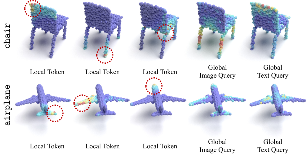
According to the design, ReCon should have learned both locally focused and global 3D geometric understandings. In Figure 7, we visualize the attention distribution of randomly selected local tokens and global queries. The red and yellow parts are the key areas of attention, while the blue and purple parts are the areas of less attention. It can be seen that the local tokens in 3D point clouds focus more on the geometric structure around the tokens themselves, while the global queries focus on the whole parts of the object. Interestingly, the local tokens may have learned some geometric understanding of symmetry. For example, the token on the left wing of the airplane also noticed the right wing. In addition, we find that global image and text queries may have learned some complementary knowledge.

6 Conclusions

In this paper, we propose contrast with reconstruct (ReCon), which enjoys the merits of both generative masked modeling and contrastive modeling, while scalable to multimodal data to facilitate stronger 3D representation learning. Our results show high-capacity data efficiency and generalizations on both pretraining and downstream representation transferring. In particular, ReCon achieves a new state-of-the-art on challenging real-world 3D object recognition. By diving deeply into ReCon, we emphasize the importance of reconstruction, which avoids the contrastive over-fitting issue due to limited 3D data. Visualizations show that ReCon indeed learns decoupled local and global representations in the proposed ReCon-block. ReCon is a simple framework, and we hope more ReCon-style models to be produced in the multi-modal learning community.

References

Afham et al. (2022) Afham, M., Dissanayake, I., Dissanayake, D., Dharmasiri, A., Thilakarathna, K., and Rodrigo, R. Crosspoint: Self-supervised cross-modal contrastive learning for 3d point cloud understanding. In IEEE/CVF Conf. Comput. Vis. Pattern Recog. (CVPR), 2022.
Alayrac et al. (2022) Alayrac, J., Donahue, J., Luc, P., Miech, A., Barr, I., Hasson, Y., Lenc, K., Mensch, A., Millican, K., Reynolds, M., Ring, R., Rutherford, E., Cabi, S., Han, T., Gong, Z., Samangooei, S., Monteiro, M., Menick, J., Borgeaud, S., Brock, A., Nematzadeh, A., Sharifzadeh, S., Binkowski, M., Barreira, R., Vinyals, O., Zisserman, A., and Simonyan, K. Flamingo: a visual language model for few-shot learning. In Adv. Neural Inform. Process. Syst. (NeurIPS), 2022.
Bachman et al. (2019) Bachman, P., Hjelm, R. D., and Buchwalter, W. Learning representations by maximizing mutual information across views. In Adv. Neural Inform. Process. Syst. (NeurIPS), 2019.
Bao et al. (2022) Bao, H., Dong, L., Piao, S., and Wei, F. Beit: BERT pre-training of image transformers. In Int. Conf. Learn. Represent. (ICLR). OpenReview.net, 2022.
Belghazi et al. (2018) Belghazi, M. I., Baratin, A., Rajeswar, S., Ozair, S., Bengio, Y., Hjelm, R. D., and Courville, A. C. Mutual information neural estimation. In Proc. Int. Conf. Mach. Learn. (ICML), volume 80 of Proceedings of Machine Learning Research, pp. 530–539. PMLR, 2018.
Bommasani et al. (2021) Bommasani, R., Hudson, D. A., Adeli, E., Altman, R., Arora, S., von Arx, S., Bernstein, M. S., Bohg, J., Bosselut, A., Brunskill, E., Brynjolfsson, E., Buch, S., Card, D., Castellon, R., Chatterji, N. S., Chen, A. S., Creel, K., Davis, J. Q., Demszky, D., Donahue, C., Doumbouya, M., Durmus, E., Ermon, S., Etchemendy, J., Ethayarajh, K., Fei-Fei, L., Finn, C., Gale, T., Gillespie, L., Goel, K., Goodman, N. D., Grossman, S., Guha, N., Hashimoto, T., Henderson, P., Hewitt, J., Ho, D. E., Hong, J., Hsu, K., Huang, J., Icard, T., Jain, S., Jurafsky, D., Kalluri, P., Karamcheti, S., Keeling, G., Khani, F., Khattab, O., Koh, P. W., Krass, M. S., Krishna, R., Kuditipudi, R., and et al. On the opportunities and risks of foundation models. CoRR, abs/2108.07258, 2021.
Boser et al. (1992) Boser, B. E., Guyon, I., and Vapnik, V. A training algorithm for optimal margin classifiers. In ACM Conf. Comput. Learn. Theory (COLT), pp. 144–152. ACM, 1992.
Brown et al. (2020) Brown, T. B., Mann, B., Ryder, N., Subbiah, M., Kaplan, J., Dhariwal, P., Neelakantan, A., Shyam, P., Sastry, G., Askell, A., Agarwal, S., Herbert-Voss, A., Krueger, G., Henighan, T., Child, R., Ramesh, A., Ziegler, D. M., Wu, J., Winter, C., Hesse, C., Chen, M., Sigler, E., Litwin, M., Gray, S., Chess, B., Clark, J., Berner, C., McCandlish, S., Radford, A., Sutskever, I., and Amodei, D. Language models are few-shot learners. In Adv. Neural Inform. Process. Syst. (NeurIPS), 2020.
Caron et al. (2021) Caron, M., Touvron, H., Misra, I., Jégou, H., Mairal, J., Bojanowski, P., and Joulin, A. Emerging properties in self-supervised vision transformers. In Int. Conf. Comput. Vis. (ICCV), pp. 9630–9640. IEEE, 2021.
Chang et al. (2015) Chang, A. X., Funkhouser, T. A., Guibas, L. J., Hanrahan, P., Huang, Q., Li, Z., Savarese, S., Savva, M., Song, S., Su, H., Xiao, J., Yi, L., and Yu, F. Shapenet: An information-rich 3d model repository. CoRR, abs/1512.03012, 2015.
Chen et al. (2020) Chen, T., Kornblith, S., Norouzi, M., and Hinton, G. E. A simple framework for contrastive learning of visual representations. In Proc. Int. Conf. Mach. Learn. (ICML), volume 119 of Proceedings of Machine Learning Research, pp. 1597–1607. PMLR, 2020.
Chen & He (2021) Chen, X. and He, K. Exploring simple siamese representation learning. In IEEE/CVF Conf. Comput. Vis. Pattern Recog. (CVPR), pp. 15750–15758, 2021.
Chen et al. (2021) Chen, X., Xie, S., and He, K. An empirical study of training self-supervised vision transformers. In Int. Conf. Comput. Vis. (ICCV), pp. 9620–9629. IEEE, 2021.
Chen et al. (2022) Chen, Y., Nießner, M., and Dai, A. 4dcontrast: Contrastive learning with dynamic correspondences for 3d scene understanding. In Eur. Conf. Comput. Vis. (ECCV), 2022.
Dangovski et al. (2022) Dangovski, R., Jing, L., Loh, C., Han, S., Srivastava, A., Cheung, B., Agrawal, P., and Soljacic, M. Equivariant self-supervised learning: Encouraging equivariance in representations. In Int. Conf. Learn. Represent. (ICLR). OpenReview.net, 2022.
Deng et al. (2009) Deng, J., Dong, W., Socher, R., Li, L., Li, K., and Fei-Fei, L. Imagenet: A large-scale hierarchical image database. In IEEE/CVF Conf. Comput. Vis. Pattern Recog. (CVPR), 2009.
Devlin et al. (2019) Devlin, J., Chang, M., Lee, K., and Toutanova, K. BERT: pre-training of deep bidirectional transformers for language understanding. In Proceedings of the 2019 Conference of the North American Chapter of the Association for Computational Linguistics: Human Language Technologies, NAACL-HLT 2019, Minneapolis, MN, USA, June 2-7, 2019, Volume 1 (Long and Short Papers), pp. 4171–4186. Association for Computational Linguistics, 2019.
Dong et al. (2023) Dong, R., Qi, Z., Zhang, L., Zhang, J., Sun, J., Ge, Z., Yi, L., and Ma, K. Autoencoders as cross-modal teachers: Can pretrained 2d image transformers help 3d representation learning? In Int. Conf. Learn. Represent. (ICLR), 2023.
Dong et al. (2022) Dong, X., Bao, J., Zhang, T., Chen, D., Gu, S., Zhang, W., Yuan, L., Chen, D., Wen, F., and Yu, N. CLIP itself is a strong fine-tuner: Achieving 85.7% and 88.0% top-1 accuracy with vit-b and vit-l on imagenet. CoRR, abs/2212.06138, 2022.
Dosovitskiy et al. (2021) Dosovitskiy, A., Beyer, L., Kolesnikov, A., Weissenborn, D., Zhai, X., Unterthiner, T., Dehghani, M., Minderer, M., Heigold, G., Gelly, S., Uszkoreit, J., and Houlsby, N. An image is worth 16x16 words: Transformers for image recognition at scale. In Int. Conf. Learn. Represent. (ICLR), 2021.
Ermolov et al. (2021) Ermolov, A., Siarohin, A., Sangineto, E., and Sebe, N. Whitening for self-supervised representation learning. In Proc. Int. Conf. Mach. Learn. (ICML), volume 139 of Proceedings of Machine Learning Research, pp. 3015–3024. PMLR, 2021.
Faghri et al. (2018) Faghri, F., Fleet, D. J., Kiros, J. R., and Fidler, S. VSE++: improving visual-semantic embeddings with hard negatives. In Brit. Mach. Vis. Conf. (BMVC), pp. 12. BMVA Press, 2018.
Fan et al. (2017) Fan, H., Su, H., and Guibas, L. J. A point set generation network for 3d object reconstruction from a single image. In IEEE/CVF Conf. Comput. Vis. Pattern Recog. (CVPR), 2017.
Goyal et al. (2021) Goyal, A., Law, H., Liu, B., Newell, A., and Deng, J. Revisiting point cloud shape classification with a simple and effective baseline. In Proc. Int. Conf. Mach. Learn. (ICML), volume 139 of Proceedings of Machine Learning Research, pp. 3809–3820. PMLR, 2021.
Goyal et al. (2019) Goyal, P., Mahajan, D., Gupta, A., and Misra, I. Scaling and benchmarking self-supervised visual representation learning. In Int. Conf. Comput. Vis. (ICCV), pp. 6390–6399. IEEE, 2019.
Grill et al. (2020) Grill, J., Strub, F., Altché, F., Tallec, C., Richemond, P. H., Buchatskaya, E., Doersch, C., Pires, B. Á., Guo, Z., Azar, M. G., Piot, B., Kavukcuoglu, K., Munos, R., and Valko, M. Bootstrap your own latent - A new approach to self-supervised learning. In Adv. Neural Inform. Process. Syst. (NeurIPS), 2020.
Guo et al. (2021) Guo, M., Cai, J., Liu, Z., Mu, T., Martin, R. R., and Hu, S. PCT: point cloud transformer. Comput. Vis. Media, 7(2):187–199, 2021.
Hadsell et al. (2006) Hadsell, R., Chopra, S., and LeCun, Y. Dimensionality reduction by learning an invariant mapping. In IEEE/CVF Conf. Comput. Vis. Pattern Recog. (CVPR), pp. 1735–1742, 2006.
Hamdi et al. (2021) Hamdi, A., Giancola, S., and Ghanem, B. MVTN: multi-view transformation network for 3d shape recognition. In Int. Conf. Comput. Vis. (ICCV), pp. 1–11. IEEE, 2021.
He et al. (2016) He, K., Zhang, X., Ren, S., and Sun, J. Deep residual learning for image recognition. In IEEE/CVF Conf. Comput. Vis. Pattern Recog. (CVPR), pp. 770–778. IEEE Computer Society, 2016.
He et al. (2020) He, K., Fan, H., Wu, Y., Xie, S., and Girshick, R. B. Momentum contrast for unsupervised visual representation learning. In IEEE/CVF Conf. Comput. Vis. Pattern Recog. (CVPR), pp. 9726–9735. Computer Vision Foundation / IEEE, 2020.
He et al. (2022) He, K., Chen, X., Xie, S., Li, Y., Dollár, P., and Girshick, R. B. Masked autoencoders are scalable vision learners. In IEEE/CVF Conf. Comput. Vis. Pattern Recog. (CVPR), 2022.
Hinton et al. (2015) Hinton, G. E., Vinyals, O., and Dean, J. Distilling the knowledge in a neural network. In Adv. Neural Inform. Process. Syst. (NeurIPS), volume abs/1503.02531, 2015.
Hjelm et al. (2019) Hjelm, R. D., Fedorov, A., Lavoie-Marchildon, S., Grewal, K., Bachman, P., Trischler, A., and Bengio, Y. Learning deep representations by mutual information estimation and maximization. In Int. Conf. Learn. Represent. (ICLR), 2019.
Huang et al. (2022) Huang, T., Dong, B., Yang, Y., Huang, X., Lau, R. W. H., Ouyang, W., and Zuo, W. Clip2point: Transfer CLIP to point cloud classification with image-depth pre-training. CoRR, abs/2210.01055, 2022.
Jing et al. (2021) Jing, L., Vahdani, E., Tan, J., and Tian, Y. Cross-modal center loss for 3d cross-modal retrieval. In IEEE/CVF Conf. Comput. Vis. Pattern Recog. (CVPR), pp. 3142–3151. Computer Vision Foundation / IEEE, 2021.
Khosla et al. (2020) Khosla, P., Teterwak, P., Wang, C., Sarna, A., Tian, Y., Isola, P., Maschinot, A., Liu, C., and Krishnan, D. Supervised contrastive learning. In Adv. Neural Inform. Process. Syst. (NeurIPS), 2020.
Kong & Zhang (2023) Kong, X. and Zhang, X. Understanding masked image modeling via learning occlusion invariant feature. In IEEE/CVF Conf. Comput. Vis. Pattern Recog. (CVPR), 2023.
Kosmann-Schwarzbach (2011) Kosmann-Schwarzbach, Y. The Noether Theorems, pp. 55–64. Springer New York, New York, NY, 2011. ISBN 978-0-387-87868-3. doi: 10.1007/978-0-387-87868-3˙3. URL https://doi.org/10.1007/978-0-387-87868-3_3.
Li et al. (2021) Li, J., Selvaraju, R. R., Gotmare, A., Joty, S. R., Xiong, C., and Hoi, S. C. Align before fuse: Vision and language representation learning with momentum distillation. In Adv. Neural Inform. Process. Syst. (NeurIPS), pp. 9694–9705, 2021.
Li et al. (2023) Li, J., Li, D., Savarese, S., and Hoi, S. C. H. BLIP-2: bootstrapping language-image pre-training with frozen image encoders and large language models. CoRR, abs/2301.12597, 2023.
Li et al. (2022a) Li, L. H., Zhang, P., Zhang, H., Yang, J., Li, C., Zhong, Y., Wang, L., Yuan, L., Zhang, L., Hwang, J., Chang, K., and Gao, J. Grounded language-image pre-training. In IEEE/CVF Conf. Comput. Vis. Pattern Recog. (CVPR), pp. 10955–10965. IEEE, 2022a.
Li et al. (2018) Li, Y., Bu, R., Sun, M., Wu, W., Di, X., and Chen, B. Pointcnn: Convolution on x-transformed points. In Adv. Neural Inform. Process. Syst. (NeurIPS), pp. 828–838, 2018.
Li et al. (2022b) Li, Y., Fan, H., Hu, R., Feichtenhofer, C., and He, K. Scaling language-image pre-training via masking. CoRR, abs/2212.00794, 2022b.
Liu et al. (2022) Liu, H., Cai, M., and Lee, Y. J. Masked discrimination for self-supervised learning on point clouds. In Eur. Conf. Comput. Vis. (ECCV), 2022.
Liu et al. (2019) Liu, Y., Fan, B., Xiang, S., and Pan, C. Relation-shape convolutional neural network for point cloud analysis. In IEEE/CVF Conf. Comput. Vis. Pattern Recog. (CVPR), pp. 8895–8904. Computer Vision Foundation / IEEE, 2019.
Liu et al. (2021a) Liu, Y., Fan, Q., Zhang, S., Dong, H., Funkhouser, T. A., and Yi, L. Contrastive multimodal fusion with tupleinfonce. In Int. Conf. Comput. Vis. (ICCV), pp. 734–743. IEEE, 2021a.
Liu et al. (2021b) Liu, Z., Lin, Y., Cao, Y., Hu, H., Wei, Y., Zhang, Z., Lin, S., and Guo, B. Swin transformer: Hierarchical vision transformer using shifted windows. In Int. Conf. Comput. Vis. (ICCV), pp. 9992–10002. IEEE, 2021b.
Loshchilov & Hutter (2017) Loshchilov, I. and Hutter, F. SGDR: stochastic gradient descent with warm restarts. In Int. Conf. Learn. Represent. (ICLR). OpenReview.net, 2017.
Loshchilov & Hutter (2019) Loshchilov, I. and Hutter, F. Decoupled weight decay regularization. In Int. Conf. Learn. Represent. (ICLR), 2019.
Ma et al. (2022) Ma, X., Qin, C., You, H., Ran, H., and Fu, Y. Rethinking network design and local geometry in point cloud: A simple residual MLP framework. In Int. Conf. Learn. Represent. (ICLR). OpenReview.net, 2022.
OpenAI (2022) OpenAI. Introducing chatgpt. 2022. URL https://openai.com/blog/chatgpt.
Ouyang et al. (2022) Ouyang, L., Wu, J., Jiang, X., Almeida, D., Wainwright, C. L., Mishkin, P., Zhang, C., Agarwal, S., Slama, K., Ray, A., Schulman, J., Hilton, J., Kelton, F., Miller, L., Simens, M., Askell, A., Welinder, P., Christiano, P. F., Leike, J., and Lowe, R. Training language models to follow instructions with human feedback. CoRR, abs/2203.02155, 2022.
Pang et al. (2022) Pang, Y., Wang, W., Tay, F. E. H., Liu, W., Tian, Y., and Yuan, L. Masked autoencoders for point cloud self-supervised learning. In Eur. Conf. Comput. Vis. (ECCV), 2022.
Park & Kwak (2020) Park, S. and Kwak, N. Feature-level ensemble knowledge distillation for aggregating knowledge from multiple networks. In Giacomo, G. D., Catalá, A., Dilkina, B., Milano, M., Barro, S., Bugarín, A., and Lang, J. (eds.), Eur. Conf. Artif. Intell. (ECAI), volume 325 of Frontiers in Artificial Intelligence and Applications, pp. 1411–1418. IOS Press, 2020.
Qi et al. (2017a) Qi, C. R., Su, H., Mo, K., and Guibas, L. J. Pointnet: Deep learning on point sets for 3d classification and segmentation. In IEEE/CVF Conf. Comput. Vis. Pattern Recog. (CVPR), pp. 77–85, 2017a.
Qi et al. (2017b) Qi, C. R., Yi, L., Su, H., and Guibas, L. J. Pointnet++: Deep hierarchical feature learning on point sets in a metric space. In Adv. Neural Inform. Process. Syst. (NIPS), pp. 5099–5108, 2017b.
Qian et al. (2022) Qian, G., Li, Y., Peng, H., Mai, J., Hammoud, H. A. A. K., Elhoseiny, M., and Ghanem, B. Pointnext: Revisiting pointnet++ with improved training and scaling strategies. In Adv. Neural Inform. Process. Syst. (NeurIPS), 2022.
Radford et al. (2018) Radford, A., Narasimhan, K., Salimans, T., Sutskever, I., et al. Improving language understanding by generative pre-training. 2018.
Radford et al. (2021) Radford, A., Kim, J. W., Hallacy, C., Ramesh, A., Goh, G., Agarwal, S., Sastry, G., Askell, A., Mishkin, P., Clark, J., Krueger, G., and Sutskever, I. Learning transferable visual models from natural language supervision. In Proc. Int. Conf. Mach. Learn. (ICML), volume 139 of Proceedings of Machine Learning Research, pp. 8748–8763. PMLR, 2021.
Ramesh et al. (2021) Ramesh, A., Pavlov, M., Goh, G., Gray, S., Voss, C., Radford, A., Chen, M., and Sutskever, I. Zero-shot text-to-image generation. In Proc. Int. Conf. Mach. Learn. (ICML), volume 139 of Proceedings of Machine Learning Research, pp. 8821–8831. PMLR, 2021.
Rombach et al. (2022) Rombach, R., Blattmann, A., Lorenz, D., Esser, P., and Ommer, B. High-resolution image synthesis with latent diffusion models. In IEEE/CVF Conf. Comput. Vis. Pattern Recog. (CVPR), pp. 10674–10685. IEEE, 2022.
Ruder (2017) Ruder, S. An overview of multi-task learning in deep neural networks. CoRR, abs/1706.05098, 2017.
Schuhmann et al. (2022) Schuhmann, C., Beaumont, R., Vencu, R., Gordon, C., Wightman, R., Cherti, M., Coombes, T., Katta, A., Mullis, C., Wortsman, M., Schramowski, P., Kundurthy, S., Crowson, K., Schmidt, L., Kaczmarczyk, R., and Jitsev, J. LAION-5B: an open large-scale dataset for training next generation image-text models. CoRR, abs/2210.08402, 2022.
Tao et al. (2022) Tao, C., Zhu, X., Huang, G., Qiao, Y., Wang, X., and Dai, J. Siamese image modeling for self-supervised vision representation learning. CoRR, abs/2206.01204, 2022.
Tian et al. (2020a) Tian, Y., Krishnan, D., and Isola, P. Contrastive multiview coding. In Vedaldi, A., Bischof, H., Brox, T., and Frahm, J. (eds.), Eur. Conf. Comput. Vis. (ECCV), volume 12356 of Lecture Notes in Computer Science, pp. 776–794. Springer, 2020a.
Tian et al. (2020b) Tian, Y., Krishnan, D., and Isola, P. Contrastive representation distillation. In Int. Conf. Learn. Represent. (ICLR), 2020b.
Tian et al. (2020c) Tian, Y., Sun, C., Poole, B., Krishnan, D., Schmid, C., and Isola, P. What makes for good views for contrastive learning? In Adv. Neural Inform. Process. Syst. (NeurIPS), 2020c.
Uy et al. (2019) Uy, M. A., Pham, Q.-H., Hua, B.-S., Nguyen, T., and Yeung, S.-K. Revisiting point cloud classification: A new benchmark dataset and classification model on real-world data. In IEEE/CVF Conf. Comput. Vis. Pattern Recog. (CVPR), pp. 1588–1597, 2019.
van den Oord et al. (2018) van den Oord, A., Li, Y., and Vinyals, O. Representation learning with contrastive predictive coding. CoRR, abs/1807.03748, 2018.
Vapnik (1998) Vapnik, V. Statistical learning theory. Wiley, 1998. ISBN 978-0-471-03003-4.
Vaswani et al. (2017) Vaswani, A., Shazeer, N., Parmar, N., Uszkoreit, J., Jones, L., Gomez, A. N., Kaiser, L., and Polosukhin, I. Attention is all you need. In Adv. Neural Inform. Process. Syst. (NIPS), pp. 5998–6008, 2017.
Wang et al. (2021) Wang, H., Liu, Q., Yue, X., Lasenby, J., and Kusner, M. J. Unsupervised point cloud pre-training via occlusion completion. In Int. Conf. Comput. Vis. (ICCV), pp. 9782–9792, 2021.
Wang & Yoon (2022) Wang, L. and Yoon, K. Knowledge distillation and student-teacher learning for visual intelligence: A review and new outlooks. IEEE Trans. Pattern Anal. Mach. Intell. (TPAMI), 44(6):3048–3068, 2022.
Wang & Qi (2021) Wang, X. and Qi, G. Contrastive learning with stronger augmentations. CoRR, abs/2104.07713, 2021.
Wang et al. (2019) Wang, Y., Sun, Y., Liu, Z., Sarma, S. E., Bronstein, M. M., and Solomon, J. M. Dynamic graph CNN for learning on point clouds. ACM Trans. Graph., 38(5):146:1–146:12, 2019.
Wang et al. (2022) Wang, Z., Yu, X., Rao, Y., Zhou, J., and Lu, J. P2P: tuning pre-trained image models for point cloud analysis with point-to-pixel prompting. In Adv. Neural Inform. Process. Syst. (NeurIPS), 2022.
Wei et al. (2022a) Wei, C., Fan, H., Xie, S., Wu, C.-Y., Yuille, A., and Feichtenhofer, C. Masked feature prediction for self-supervised visual pre-training. In IEEE/CVF Conf. Comput. Vis. Pattern Recog. (CVPR), 2022a.
Wei et al. (2022b) Wei, J., Wang, X., Schuurmans, D., Bosma, M., brian ichter, Xia, F., Chi, E. H., Le, Q. V., and Zhou, D. Chain of thought prompting elicits reasoning in large language models. In Adv. Neural Inform. Process. Syst. (NeurIPS), 2022b.
Wu et al. (2015) Wu, Z., Song, S., Khosla, A., Yu, F., Zhang, L., Tang, X., and Xiao, J. 3d shapenets: A deep representation for volumetric shapes. In IEEE/CVF Conf. Comput. Vis. Pattern Recog. (CVPR), pp. 1912–1920, 2015.
Wu et al. (2018) Wu, Z., Xiong, Y., Yu, S. X., and Lin, D. Unsupervised feature learning via non-parametric instance discrimination. In IEEE/CVF Conf. Comput. Vis. Pattern Recog. (CVPR), pp. 3733–3742. Computer Vision Foundation / IEEE Computer Society, 2018.
Xiang et al. (2020) Xiang, L., Ding, G., and Han, J. Learning from multiple experts: Self-paced knowledge distillation for long-tailed classification. In Eur. Conf. Comput. Vis. (ECCV), volume 12350 of Lecture Notes in Computer Science, pp. 247–263. Springer, 2020.
Xie et al. (2020) Xie, S., Gu, J., Guo, D., Qi, C. R., Guibas, L. J., and Litany, O. Pointcontrast: Unsupervised pre-training for 3d point cloud understanding. In Eur. Conf. Comput. Vis. (ECCV), volume 12348 of Lecture Notes in Computer Science, pp. 574–591. Springer, 2020.
Xie et al. (2022a) Xie, Z., Geng, Z., Hu, J., Zhang, Z., Hu, H., and Cao, Y. Revealing the dark secrets of masked image modeling. CoRR, abs/2205.13543, 2022a.
Xie et al. (2022b) Xie, Z., Zhang, Z., Cao, Y., Lin, Y., Wei, Y., Dai, Q., and Hu, H. On data scaling in masked image modeling. CoRR, abs/2206.04664, 2022b.
Yi et al. (2016) Yi, L., Kim, V. G., Ceylan, D., Shen, I.-C., Yan, M., Su, H., Lu, C., Huang, Q., Sheffer, A., and Guibas, L. A scalable active framework for region annotation in 3d shape collections. ACM Trans. Graph., 35(6):1–12, 2016.
Yu et al. (2022a) Yu, J., Wang, Z., Vasudevan, V., Yeung, L., Seyedhosseini, M., and Wu, Y. Coca: Contrastive captioners are image-text foundation models. Trans. Mach. Learn. Res. (TMLR), 2022a. ISSN 2835-8856.
Yu et al. (2022b) Yu, X., Tang, L., Rao, Y., Huang, T., Zhou, J., and Lu, J. Point-bert: Pre-training 3d point cloud transformers with masked point modeling. In IEEE/CVF Conf. Comput. Vis. Pattern Recog. (CVPR), 2022b.
Zbontar et al. (2021) Zbontar, J., Jing, L., Misra, I., LeCun, Y., and Deny, S. Barlow twins: Self-supervised learning via redundancy reduction. In Proc. Int. Conf. Mach. Learn. (ICML), volume 139 of Proceedings of Machine Learning Research, pp. 12310–12320. PMLR, 2021.
Zhang et al. (2022a) Zhang, L., Chen, X., Zhang, J., Dong, R., and Ma, K. Contrastive deep supervision. In Eur. Conf. Comput. Vis. (ECCV), volume 13686 of Lecture Notes in Computer Science, pp. 1–19. Springer, 2022a.
Zhang et al. (2022b) Zhang, R., Guo, Z., Gao, P., Fang, R., Zhao, B., Wang, D., Qiao, Y., and Li, H. Point-m2AE: Multi-scale masked autoencoders for hierarchical point cloud pre-training. In Adv. Neural Inform. Process. Syst. (NeurIPS), 2022b.
Zhang et al. (2022c) Zhang, R., Guo, Z., Zhang, W., Li, K., Miao, X., Cui, B., Qiao, Y., Gao, P., and Li, H. Pointclip: Point cloud understanding by CLIP. In IEEE/CVF Conf. Comput. Vis. Pattern Recog. (CVPR), 2022c.
Zhang et al. (2021) Zhang, Z., Girdhar, R., Joulin, A., and Misra, I. Self-supervised pretraining of 3d features on any point-cloud. In Int. Conf. Comput. Vis. (ICCV), pp. 10232–10243. IEEE, 2021.
Zhou et al. (2022) Zhou, J., Wei, C., Wang, H., Shen, W., Xie, C., Yuille, A. L., and Kong, T. ibot: Image BERT pre-training with online tokenizer. In Int. Conf. Learn. Represent. (ICLR), 2022.

Appendix A Additional Related Works

Contrastive-Generative Representation Learning In 2D vision and NLP, some works have been proposed for contrastive-generative representation learning. Zhou et al. 2022 propose to use an online tokenizer to distill local tokens and global class tokens, respectively. Tao et al. 2022 further proposes to perform three tasks at the same time: reconstruction, intra-view matching, and intra-image contrastive learning. This paradigm is also trending in the vision-language (VL) community, Li et al. 2021 propose ALBEF that uses contrastive learning before modality fusion to make the reconstructed features encoded with more semantics. Through cross attention of different modalities, CoCa (Yu et al. 2022a) fuses visual-language features while performing mask language modeling, where contrastive learning aligns the multi-modal global features. Recently, Li et al. 2022b propose to use masked signals for contrastive VL learning, which greatly improves the training efficiency without losing performance. Different from these methods, our ReCon is built for 3D representation learning, which is faced with a unique and serious low-data challenge. Besides, we propose a novel ReCon-block that models contrastive-generative representation learning as a generative pretraining guided contrastive learning.

Table 7: Training recipes for pretraining and downstream fine-tuning.

	Pretraining	Classification		Segmentation
Config	ShapeNet	ScanObjectNN	ModelNet	ShapeNetPart
optimizer	AdamW	AdamW	AdamW	AdamW
learning rate	5e-4	2e-5	1e-5	2e-4
weight decay	5e-2	5e-2	5e-2	5e-2
learning rate scheduler	cosine	cosine	cosine	cosine
training epochs	300	300	300	300
warmup epochs	10	10	10	10
batch size	128	32	32	16
drop path rate	0.1	0.2	0.2	0.1
image resolution	224 $\times$ 224	-	-	-
image patch size	16	-	-	-
number of points	1024	2048	1024/8192	2048
number of point patches	64	128	64/512	128
point patch size	32	32	32	32
augmentation	Rotation	Rotation	Scale&Trans	-
GPU device	PH402 SKU 200	RTX 2080Ti	RTX 2080Ti	RTX 2080Ti

Appendix B Additional Implementation Details

B.1 Loss Function

In this section, we detail the loss functions in our implementation of contrastive models, generative models, and our ReCon models. Given a randomly sampled multimodal minibatch $\{\mathbf{p}_{k},\mathbf{i}_{k},\mathbf{t}_{k}\}_{k=1}^{N}$ with $N$ paired samples, where $\mathbf{p}_{k}$ is the $k$ -th 3D point cloud sample, and $\mathbf{i}_{k}$ , $\mathbf{t}_{k}$ are the corresponding multimodal views, i.e., rendered RGB image (rendered from the single view of the default pose) and text category description (e.g., chair), respectively. By dividing the text category descriptions into $K$ groups $\{T_{k}\}_{k=1}^{K}$ where $T_{k}$ is the $k$ -th unique text description, we obtain a fine-grained label set $\{\mathbf{y}_{k}=\ell:\mathbf{t}_{k}=T_{\ell}\}_{k=1}^{N}$ of ShapeNet. Hence, the minibatch becomes $\{\mathbf{p}_{k},\mathbf{i}_{k},\mathbf{t}_{k},\mathbf{y}_{k}\}_{k=1}^{N}$ , and we can use part of them or all of them to perform different self-supervised representation learning methods.

Single-Modal Contrastive Loss For the single-modal contrastive models (SMC), we use a supervised contrastive loss following Khosla et al. 2020, where the supervision is generalized from the constructed label set. Let $k\in\mathcal{K}\equiv\{1,\dots,N\}$ be the index of the minibatch samples where $\mathcal{A}_{k}=\mathcal{K}\backslash\{k\}$ is the index set for all samples other than the $k$ -th anchor sample. $\mathcal{P}_{k}\equiv\{p\in\mathcal{A}_{k}:\mathbf{y}_{p}=\mathbf{y}_{k}\}$ is the index for the positive samples, and other samples with different labels are considered as the negative samples. Given the 3D student network $\mathcal{F}^{\text{P}}(\cdot)$ , where $z^{\text{P}}_{\ell}=\mathcal{F}^{\text{P}}(\mathbf{p}_{\ell}),\ell\in\mathcal{K}$ . The loss $\mathcal{L}^{\text{SMC}}$ can be written as:

\mathcal{L}^{\text{SMC}}=\sum_{k\in\mathcal{K}}\frac{-1}{|\mathcal{P}_{k}|}\sum_{p\in\mathcal{P}_{k}}\log\frac{\exp(z^{\text{P}}_{k}\cdot z^{\text{P}}_{p}/\tau)}{\mathop{\sum}\limits_{a\in\mathcal{A}_{i}}\exp(z^{\text{P}}_{k}\cdot z^{\text{P}}_{a}/\tau)},

(4)

where $\tau\in\mathbb{R}$ is the scalar temperature parameter which is set as 0.1 (Khosla et al. 2020) for all contrastive models.

Cross-Modal Contrastive Loss For the cross-modal contrastive models (CMC), we use the contrastive InfoNCE loss (van den Oord et al. 2018) following Radford et al. 2021. Given the minibatch, we can construct two groups of $N\times N$ pairs, i.e., point-image pairs $\big\{\{\mathbf{p}_{m},\mathbf{i}_{n}\}:\forall m\in\mathcal{K},\forall n\in\mathcal{K}\big\}$ and point-text pairs $\big\{\{\mathbf{p}_{m},\mathbf{t}_{n}\}:\forall m\in\mathcal{K},\forall n\in\mathcal{K}\big\}$ . Then the encoded representation of another modality from the same sample is used as positive, while the others in the minibatch are used as negative samples. Given a pretrained 2D teacher network $\mathcal{F}^{\text{I}}(\cdot)$ and a pretrained language teacher network $\mathcal{F}^{\text{T}}(\cdot)$ , where $z^{\text{I}}_{\ell}=\mathcal{F}^{\text{I}}(\mathbf{i}_{\ell}),\ell\in\mathcal{K}$ and $z^{\text{T}}_{\ell}=\mathcal{F}^{\text{T}}(\mathbf{t}_{\ell}),\ell\in\mathcal{K}$ represent the decoded representations, respectively. Similar to Eq. (4), the loss $\mathcal{L}^{\text{CMC}}$ is the summation of multimodal point-image loss $\mathcal{L}^{\text{CMC-PI}}$ and point-text loss $\mathcal{L}^{\text{CMC-PT}}$ :

\mathcal{L}^{\text{CMC}}=-\sum_{k\in\mathcal{K}}\left[\underbrace{\log\frac{\exp\left(z^{\text{P}}_{k}\cdot\texttt{stopgrad}(z^{\text{I}}_{k})/\tau\right)}{\mathop{\sum}\limits_{a\in\mathcal{A}_{i}}\exp(z^{\text{P}}_{k}\cdot z^{\text{I}}_{a}/\tau)}}_{\mathcal{L}^{\text{CMC-PI}}}+\underbrace{\log\frac{\exp\left(z^{\text{P}}_{k}\cdot\texttt{stopgrad}(z^{\text{T}}_{k})/\tau\right)}{\mathop{\sum}\limits_{a\in\mathcal{A}_{i}}\exp(z^{\text{P}}_{k}\cdot z^{\text{T}}_{a}/\tau)}}_{\mathcal{L}^{\text{CMC-PT}}}\right],

(5)

where $\tau\in\mathbb{R}$ is the scalar temperature parameter, and $\texttt{stopgrad}(\cdot)$ is the stop-gradient operation. Here, no gradient is back-propagated to the image or text teachers, and hence the two cross-modal teachers are frozen.

Masked Point Modeling Reconstruction Loss For the masked point modeling reconstruction (MPM), we use the $\ell_{2}$ Chamfer-Distance (Fan et al. 2017) following Pang et al. 2022. Denote $\mathcal{M}_{\ell}(\cdot),\ell\in\mathcal{K}$ as the masking operation. Let $\mathcal{R}_{\ell}\equiv\mathcal{F}^{\text{P}}\big(\mathcal{M}_{\ell}(\mathbf{p}_{\ell})\big),\ell\in\mathcal{K}$ and $\mathcal{G}_{\ell}\equiv\mathbf{p}_{\ell},\ell\in\mathcal{K}$ be the reconstructed point clouds and ground truth point clouds, respectively. The reconstruction loss $\mathcal{L}^{\text{MPM}}$ can be written as:

\mathcal{L}^{\text{MPM}}=\sum_{k\in\mathcal{K}}\left[\frac{1}{|\mathcal{R}_{k}|}\sum_{r\in\mathcal{R}_{k}}\mathop{\min}\limits_{g\in\mathcal{G}_{k}}\|r-g\|^{2}_{2}+\sum_{g\in\mathcal{G}_{k}}\mathop{\min}\limits_{r\in\mathcal{R}_{k}}\|r-g\|^{2}_{2}\right].

(6)

ReCon Loss The ReCon loss is the ensemble distillation as defined in Eq. 3. The first term $\mathcal{L}^{\text{REC}}$ is the same as Eq. 6, and the contrastive loss can be either single-modal contrastive loss defined in Eq. 4 or the cross-modal contrastive loss defined in Eq. 5. Similar to SimSiam (Chen & He 2021), we find that the 3D student learning from the frozen cross-modal teachers with stop-gradient does not fall into the representation collapsing trap. Therefore, we use the positive-only representation learning with Smooth $\ell_{1}$ loss $\text{Smooth-}\ell_{1}(\cdot,\cdot)$ , which we find achieves the best performance (see Sec. 4.2). In this case, the cross-modal contrastive term $\mathcal{L}^{\text{CON}}$ can be written as follows:

\mathcal{L}^{\text{CON}}=\sum_{k\in\mathcal{K}}\Big[\text{Smooth-}\ell_{1}\big(z^{\text{P}}_{k},\texttt{stopgrad}(z^{\text{I}}_{k})\big)+\text{Smooth-}\ell_{1}\big(z^{\text{P}}_{k},\texttt{stopgrad}(z^{\text{T}}_{k})\big)\Big].

(7)

B.2 Experimental Details

Pretraining Details We use ShapeNetCore from ShapeNet (Chang et al. 2015) as the pretraining dataset. ShapeNet is a clean set of 3D CAD object models with rich annotations, including $\sim$ 51K unique 3D models from 55 common object categories. For the generation of paired data, we take surface point samples of the 3D object model to generate 3D point clouds, the 3D models are lighted with textures for rendering 2D RGB images. Specifically, we use the MacOS Preview⁶⁶ 6 https://en.wikipedia.org/wiki/Preview_(macOS) to generate high-quality rendered images. The text description comprises category labels and manually designed prompt templates. During pretraining, a unique image query [IMG] token and text query [TXT] token are trained to align the global representation from the image teacher and the text teacher, respectively. The overall pretraining includes 300 epochs, and we use a cosine learning rate (Loshchilov & Hutter 2017) of 5e-4 warming up for 10 epochs. AdamW optimizer (Loshchilov & Hutter 2019) is used, and the batch size is 128. More details are shown in Table 7.

Downstream Transferring Details Fig. 8 shows the pipeline when ReCon transfers to downstream tasks, including zero-shot and fine-tuning. For zero-shot, we use simple summation to fuse multi-modal features, and the cosine similarity is used as the classification metric (Radford et al. 2021). During fine-tuning, we concatenate the pooled representation of local tokens and the learned global query tokens as model features. For classification, we add a new global classification [CLS] token and concatenate it with the other queries before being fused to the classification head. It is worth noting that due to the consistency of the optimization objective during fine-tuning, we cancel the stop gradient of the cross attention connections. Without specifications, we report overall accuracy (OA) results without voting on the most challenging ScanObjectNN PB_T50_RS benchmark using 2,048 input points and ModelNet40 using 1,024 input points (1k P), and the zero-shot classification results are reported on the test split. More detailed training configurations are shown in Table 7.

Model Variants Table 8 summarizes the ReCon model configurations, which are grounded in a similar fashion of ViT variants (Dosovitskiy et al. 2021). The default version “ReCon” (or ReCon-Base) is directly adopted from previous works (Pang et al. 2022; Dong et al. 2023), except that the network is configured as two-stream rather than single-stream. We add the smaller “Tiny” and “Small” models, which have the same number of layers but with reduced channel dimension.

Table 8: Details of ReCon model variants. This table format follows Dosovitskiy et al. 2021.

Model	Layers	Hidden size	MLP size	Heads	#Params
$\bullet$ ReCon-Tiny	12	192	768	3	11.4M
$\bullet$ ReCon-Small	12	256	1024	4	19.0M
$\bullet$ ReCon	12	384	1536	6	43.6M

Appendix C Additional Baselines

We show two additional simple fusion methods (Ruder 2017), including Vanilla Multi-task Learning and a Two-Tower network. Here, we make an analysis of these two baseline methods.

Vanilla Multi-task Learning Fusion As shown in Fig. 9(a), Vanilla Multi-task Learning directly shares a standard Transformer as the encoder. The input embedding tokens take masked reconstruction as the pretext task, and the global tokens take the global contrast as the pretext task. Vanilla Multi-task Learning doesn’t consider the pattern difference issue of the two tasks (see Fig. 1 and Fig. 7). The transfer performances of Vanilla Multi-task Learning on ScanObjectNN and ModelNet40 are reported in Table 9. It is observed that this vanilla design leads to limited performance, which only improves the from scratch OA by +0.89% on ScanObjectNN, and no improvement on ModelNet40 is achieved. This indicates task conflicts, and it is consistent with the analysis in Sec. 1 that it is non-trivial for joint learning of these two tasks.

Two-Tower Network To verify whether the performance improvement of ReCon comes from the form of a two-tower architecture, we design a simple Two-Tower network, shown in Fig. 9(b). The Two-Tower network uses standard Transformers as the encoder for masked reconstruction and global contrastive learning, respectively. During fine-tuning, it concatenates features from both streams for an ensemble (similar to Fig. 8(b)). Clearly, the Two-Tower network doesn’t suffer the pattern difference issue. The transfer performances of the Two-Tower network on ScanObjectNN and ModelNet40 are reported in Table 9. It can be seen that the Two-Tower network brings unsatisfactory performance, i.e., only +3.41% and +0.5% accuracy improvements by the from scratch baseline. In comparison, our ReCon uses the reconstruction task as guidance for global contrastive learning. As a result, ReCon successfully disentangles the two tasks while preserving both merits, and significantly better improvements are achieved.

Table 9: Study of the additional baseline. Overall accuracy (%) without voting is reported.

Method	ScanObjectNN	ModelNet40
Vanilla Multi-task Learning	82.53	91.6
Two-Tower Network	85.05	92.1
ReCon	90.63	94.1

Appendix D Additional Experiments

D.1 Additional Evaluations

Linear SVM Evaluation Linear SVM evaluation (Boser et al. 1992; Vapnik 1998) can be used to evaluate the discriminative quality of pretrained features (Goyal et al. 2019). The results on ModelNet40 are shown in Table 10. It shows that our ReCon outperforms Point-BERT, which also uses plain Transformers, by a clear margin of +6.0%. Compared to methods using hierarchical Transformers, our ReCon outperforms PointM2AE (Zhang et al. 2022b) by +0.5%.

Table 10: Linear SVM classification on ModelNet40. Overall accuracy (%) without voting is reported.

Method	Hierachical	ModelNet40
$\bullet$ Point-BERT (Yu et al. 2022b)	$\times$	87.4
$\mathbf{\circ}$ OcCo (Wang et al. 2021)	$\checkmark$	89.2
$\mathbf{\circ}$ CrossPoint (Afham et al. 2022)	$\checkmark$	91.2
$\mathbf{\circ}$ PointM2AE (Zhang et al. 2022b)	$\checkmark$	92.9
$\bullet$ ReCon	$\times$	93.4

3D Part Segmentation To evaluate the geometric understanding performance within objects, we conduct the part segmentation experiment on ShapeNetPart (Yi et al. 2016). Specifically, we concatenate the cross-modal feature of ReCon into the global feature and use the same segmentation head as Point-MAE for a fair comparison. From Table 11, it can be observed that ReCon improves the from scratch baseline by +1.4% and +1.7% Cls. mIoU and Inst. mIoU, respectively. Besides, ReCon outperforms the SSL counterpart Point-MAE (Pang et al. 2022) by +0.4% Inst. mIoU. It shows that the cross-modal global knowledge from ReCon cross-modal pretraining can still play a certain role in part segmentation.

Table 11: Part segmentation on ShapeNetPart dataset. The mIoU over all classes (Cls.) and the mIoU over all instances (Inst.) are reported. ^† denotes results with our proposed

\bullet

ReCon-block built backbone architecture.

Methods	Cls. mIoU (%)	Inst. mIoU (%)
$\mathbf{\circ}$ PointNet (Qi et al. 2017a)	80.4	83.7
$\mathbf{\circ}$ PointNet++ (Qi et al. 2017b)	81.9	85.1
$\mathbf{\circ}$ DGCNN (Wang et al. 2019)	82.3	85.2
$\mathbf{\circ}$ PointMLP (Ma et al. 2022)	84.6	86.1
$\bullet$ Transformer (Vaswani et al. 2017)	83.4	84.7
$\bullet$ Transformer^† (Vaswani et al. 2017)	83.6	85.2
$\mathbf{\circ}$ PointContrast (Xie et al. 2020)	-	85.1
$\mathbf{\circ}$ CrossPoint (Afham et al. 2022)	-	85.5
$\bullet$ Point-BERT (Yu et al. 2022b)	84.1	85.6
$\bullet$ Point-MAE (Pang et al. 2022)	-	86.1
$\bullet$ Point-MAE^† (Pang et al. 2022)	84.4	86.1
$\bullet$ ACT (Dong et al. 2023)	84.7	86.1
$\bullet$ ReCon	84.8	86.4

Zero-Shot Recognition on Real-World Dataset In Table 12, we show the zero-shot evaluation results on the real-world ScanObjectNN dataset. Though our ReCon is pretrained on the synthetic dataset ShapeNet, it outperforms PointCLIP and CLIP2Point, which leverage depth images, by a clear margin. For example, on the most challenging PB_T50_RS benchmark, ReCon achieves a Top-1 accuracy of 30.5%, which is +7.2% and +15.1% higher than CLIP2Point and PointCLIP, respectively.

Table 12: Zero-shot 3D object classification on ScanObjectNN dataset. Top-1 accuracy (%) is reported. Ensemb. denotes whether to use the ensemble strategy with multiple text inputs.

Method	Backbone	Ensemb.	OBJ_ONLY	OBJ_BG	PB_T50_RS
$\mathbf{\circ}$ PointCLIP (Zhang et al. 2022c)	ResNet-50	$\times$	21.3	19.3	15.4
$\bullet$ CLIP2Point (Huang et al. 2022)	Transformer	$\checkmark$	35.5	30.5	23.3
$\bullet$ ReCon	Transformer	$\times$	39.6	38.0	29.5
$\bullet$ ReCon	Transformer	$\checkmark$	43.7	40.4	30.5

D.2 Additional Ablation Study

Data Augmentation We study the impact of using different data augmentations (DA) when fine-tuning ReCon pretrained models on different downstream tasks, as shown in Table 13. The results show that Rotation has the best performance improvement on ScanObjectNN, and Scale&Translate has the highest performance improvement on ModelNet40. Therefore, we use by default Rotation on ScanObjectNN and Scale&Translate on ModelNet40 if without specifications.

Table 13: Ablation study of data augmentations (DA) during fine-tuning. We report the fine-tuning overall accuracy (%) without voting of ReCon pretrained models.

DA Strategy	ScanObjectNN	ModelNet40
-	87.44	93.4
Scale & Translate	87.02	94.1
Jitter	90.22	92.9
Rotation	90.63	92.3
Dropout	87.40	93.5
Horizontal Flip	87.27	93.6

Paired Data Ablation During pretraining, we use the point cloud, rendered image, and text inputs generated from ShapeNet (Chang et al. 2015), which makes the data contain clear matching attributes. To verify the dependence of ReCon on paired data, we shuffle the rendered images under the same category for pretraining. The results are shown in Table 14. It shows that ReCon has a performance degradation of less than 1% in fine-tuning tasks and 6.4% in the zero-shot tasks.

Table 14: Ablation study on the paired data during pretraining. Paired denotes the paired 3D point clouds, rendered images, and category text descriptions; unpaired data denotes data with shuffled images under the same category. Overall accuracy (%) without voting is reported. ModelNet40-FT represents the fine-tuning accuracy, and ModelNet40-ZS is the zero-shot result on the train+test split.

Paired	ScanObjectNN	ModelNet40-FT	ModelNet40-ZS
$\times$	90.22	93.8	60.4
$\checkmark$	90.63	94.5	66.8

Prompt Ablation For zero-shot evaluation, we construct the prompt by concatenating the prefix prompt [P] with the category text description [C], followed by a suffix [S], and the final prompt is [P]+[C]+[C]. For example, A point cloud of a chair with white background. Table 15 shows the ablation study of results with only the prefix or suffix prompts we used, i.e., 20 prefixes and 4 suffixes. Note that when we use the ensemble strategy, the results are ensembled by all the combinations of prefixes and suffixes. The prompts can also be constructed from rendered images by powerful Vison-Language Foundation Models such as BLIP-2 (Li et al. 2023), which may further bring improvements.

Table 15: Ablation study on the prompts for zero-shot learning. [C] denotes the category text description, [P] denotes the prefix prompt, and [S] denotes the suffix prompt. Acc. (%) represents the ModelNet40 zero-shot Top-1 Accuracy (%).

[P]+[C]	Acc. (%)	[C]+[S]	Acc. (%)
‘’ + [C]	-	[C] +‘’	-
‘A ’ + [C]	52.27	[C] +‘.’	49.11
‘A model of ’ + [C]	53.04	[C] +‘ with white background.’	56.93
‘A model of a ’ + [C]	54.05	[C] +‘ with black context.’	60.57
‘An image of ’ + [C]	57.50	-	-
‘An image of a ’ + [C]	56.36	-	-
‘A 3D model of ’ + [C]	55.63	-	-
‘A 3D model of a ’ + [C]	55.71	-	-
‘A rendered model of ’ + [C]	56.48	-	-
‘A rendered model of a ’ + [C]	56.52	-	-
‘A point cloud of ’ + [C]	52.71	-	-
‘A point cloud of a ’ + [C]	55.27	-	-
‘A point cloud model of’ + [C]	56.65	-	-
‘A point cloud model of a ’ + [C]	54.46	-	-
‘A 3D rendered model of ’ + [C]	55.83	-	-
‘A 3D rendered model of a ’ + [C]	54.78	-	-
‘A rendered image of ’ + [C]	58.79	-	-
‘A rendered image of a ’ + [C]	56.48	-	-
‘A 3D rendered image of ’ + [C]	59.07	-	-
‘A 3D rendered image of a ’ + [C]	57.70	-	-

Pretraining Learning Rate Ablation on Contrastive Models

As discussed before, contrastive models can easily fall into the representation over-fitting trap. We find that it generally leads to a sensitivity to the pretraining learning rate. As shown in Table 16, when using the default learning rate for ReCon pretraining (i.e., 5e-4), the contrastive model fails to generalize with unsatisfactory results. And when the learning rate is small, where the model learns slowly, a relatively better generalization performance is achieved with improved training stability (see Fig. 6 and the discussions). We speculate that it is due to the low-data challenge, which largely makes the model easily learn over-fitted representations. As a result, the contrastive models are very sensitive to the pretraining learning rate, which has to be carefully adjusted. Hence, without specifications, we use this adjusted smaller learning rate for contrastive models.

Table 16: Ablation study on the pretraining learning rate (LR) of contrastive models. We show the results of fine-tuned cross-modal contrastive models that are pretrained with different LRs. Overall accuracy (%) without voting is reported.

LR	ScanObjectNN	ModelNet40
5e-5	85.11	92.1
1e-4	86.49	92.4
5e-4	82.48	90.3
1e-3	67.45	86.3

Ablation Study on Freezing Cross-Modal Teachers

Unlike CLIP (Radford et al. 2021), ReCon uses frozen cross-modal teachers in contrastive learning to acquire the dark knowledge of other modalities. We show the influence of freezing parameters on downstream tasks in Table 17. It can be seen that if the model uses the InfoNCE (van den Oord et al. 2018) loss function containing negative pairs, the impact of unfrozen parameters during pretraining is not significant. In contrast, for contrastive learning with only positive pairs, unfrozen parameters will cause serious performance degradation on ScanObjectNN and ModelNet.

Table 17: Ablation study on the freezing cross-modal teachers. Freeze denotes whether both image and text teachers are frozen or not. Overall accuracy (%) without voting is reported.

Freeze	Contrastive Metric	ScanObjectNN	ModelNet40
$\times$	InfoNCE	89.87	93.7
$\times$	Smooth $\ell_{1}$	84.77	91.2
$\checkmark$	InfoNCE	90.11	93.8
$\checkmark$	Smooth $\ell_{1}$	90.63	94.1

Training Costs

We report the singe-GPU without distributed training GPU hours and GPU memory usage of ReCon and Point-MAE during pretraining and fine-tuning. We study ReConwith three network configurations: ReCon, ReCon-Small, and ReCon, which are described in Table 8. Although the parameter count of ReCon is almost doubled compared to Point-MAE, the memory consumption is mainly for storing intermediate variables of the model. However, ReCon only adds three global queries to its intermediate variables compared to Point-MAE. Therefore, the memory consumption of ReCon has mostly stayed the same compared to Point-MAE.

Table 18: Training costs comparison. We report the single-GPU training GPU hours and GPU memory costs during pretraining on ShapeNet and fine-tuning on ScanObjectNN.

Method	#Params	GFLOPS	Pretrain GPU Hours	Fine-tune GPU Hours	GPU Memory	ScanObjectNN
$\bullet$ Point-MAE	22.1M	4.8	32.7h	5.3h	7766MB	85.18
$\bullet$ ReCon-Tiny	11.4M	2.4	40.9h	3.8h	4578MB	89.10
$\bullet$ ReCon-Small	19.0M	3.2	46.3h	4.5h	4710MB	89.52
$\bullet$ ReCon	43.6M	5.3	54.5h	6.1h	7906MB	90.63

Edge Device Deployments

We deploy the models using ONNX⁷⁷ 7 https://onnx.ai/ and tested it on several common edge devices, including laptops, pads, smartphones, and single chip microcomputers (SCM), all of which are tested on CPU. Table 19 shows the number of frames per second (FPS) the model can make with inputs from the ModelNet40 dataset, which uses 1K point clouds per sample. The results demonstrate that our ReCon network is easy to be deployed on various edge devices. For example, our small variant ReCon-Tiny is even more efficient that surpasses the widely used PointNet++.

Table 19: Real-time deployments on edge devices. We report the number of frames per second (FPS).

Device	Macbook Air	HUAWEI MatePad Pro	Honor X30 Android	Raspberry Pi 3B
	Laptop	Pad	Smartphone	Single Chip Microcomputer
	Apple M2 Silicon	Hisilicon Kirin 990	Qualcomm Snapdragon 695	Broadcom BCM2837
$\mathbf{\circ}$ PointNet++	83.6	25.6	16.7	2.5
$\bullet$ Point-MAE	58.7	17.8	12.8	2.1
$\bullet$ ReCon-Tiny	103.5	29.8	20.2	3.7
$\bullet$ ReCon-Small	78.1	24.5	14.6	2.7
$\bullet$ ReCon	51.7	15.6	8.1	1.8

Appendix E Discussions on Cross-Modal Teachers and Multimodal Training

In Table 20, we conduct an ablation study on pretrained teachers and multimodal data during pretraining. This analysis clearly demonstrates that (i) ReCon+SMC that leverages single-modal contrastive learning still exhibits excellent performance on downstream tasks without including any other modality data or pretrained teachers. It achieves an overall accuracy of 89.73% on ScanObjectNN, which is +1.31% better than the generative-only baseline Point-MAE and +0.72% better than the generative method ACT that leverages a pretrained 2D teacher. It demonstrates that our design of generative guidance for contrastive modeling is critical and essential for combining the merits of these two paradigms, which already yields superior results compared to other methods and has well tackled the raised issues. (ii) ReCon+CMC (from scratch) uses cross-modal contrastive learning on multimodal data while without any pretrained teachers, further bringing an improvement of +0.59% to a remarkable 90.32% overall accuracy on ScanObjectNN. It demonstrates that multimodal data is beneficial since 3D data are seriously lacking. (iii) ReCon+CMC uses cross-modal contrastive learning with both multimodal data and pretrained teachers, further leading to an improvement of +0.31% on ScanObjectNN. It demonstrates that pretrained teachers from other modality data and the usage of multimodal data in ReCon (not for other methods) can indeed further improve the performance for tackling the data dessert issue. (iv) Vanilla Multi-Task Learning and Two-Tower Network baselines that simply transfer cross-modal knowledge from pretraining weights do not produce satisfactory results. We speculate that this is due to the pattern differences issue demonstrated in Fig. 1, which is precisely the motivation behind our ReCon-block. In contrast, our ReCon+CMC outperforms these two baselines by a large margin. This shows that the benefits do not merely come from pretrained teachers but rather the fact that ReCon design is an effective framework that guides contrastive learning with generative modeling. It also shows that pretrained teachers are not all you need, and the benefits of pretrained teachers or multimodal data can not be obtained without our proposed ReCon.

Table 20: Ablation study on pretrained teachers and multimodal data. Pretrained Teacher denotes whether a pretrained teacher is used, and Multimodal Data denotes whether multimodal data is used during pretraining. SMC and CMC denote single-modal and cross-modal contrastive modeling methods, respectively. All results except the Vanilla Multi-Task Learning and Two-Tower Network baselines are conducted with our proposed

\bullet

ReCon-block built backbone architecture during fine-tuning for a fair comparison. Overall accuracy (%) without voting is reported.

Method	Pretrained Teacher	Multimodal Data	ScanObjectNN	ModelNet40
Contrastive Methods
$\bullet$ SMC Only	$\times$	$\times$	81.70	91.2
$\bullet$ CMC Only	$\checkmark$	$\checkmark$	82.48	91.4
Generative Methods
$\bullet$ Point-MAE (Pang et al. 2022)	$\times$	$\times$	88.42	93.5
$\bullet$ ACT (Dong et al. 2023)	$\checkmark$	$\times$	89.01	93.5
Generative + Contrastive Methods
Vanilla Multi-task Learning	$\checkmark$	$\checkmark$	82.53	91.6
Two-Tower Network	$\checkmark$	$\checkmark$	85.05	92.1
$\bullet$ ReCon+ SMC	$\times$	$\times$	89.73	94.0
$\bullet$ ReCon+ CMC (from scratch)	$\times$	$\checkmark$	90.32	94.0
$\bullet$ ReCon+ CMC	$\checkmark$	$\checkmark$	90.63	94.1

Appendix F Limitations and Future Works

ReCon is a general multimodal representation learning framework that leverages both merits of contrastive and generative modeling, which is demonstrated effective in 3D but is also general to any other modalities. However, there are some limitations of ReCon, which may be two-fold. (i) The first limitation may come from the multimodal data and domain. This paper mainly explores ReCon in 3D representation learning, and future explorations on multimodal problems like 2D Vision-Language may be intriguing. (ii) Another limitation may come from the architecture design, i.e., the ReCon-block proposed in this work. It is our future exploration to extend ReCon to be architecture-agnostic.

Broader Impact

The proposed ReCon is a general framework that can be used for not only 3D representation learning but also all multimodal learning problems. For example, by leveraging large-scale multimodal data like from the web (Schuhmann et al. 2022), one may obtain a foundational VL ReCon that shares a similar property of CLIP (Radford et al. 2021) since a multimodal alignment contrastive learning is used. Besides, with the rapid development of Large Language Models (LLMs), ReCon may also enable the potential for leveraging LLM like ChatGPT (OpenAI 2022) for LLM-assisted multimodal understanding. Since ReCon successfully unifies generative and contrastive modeling in a decent fashion, future applications may also involve AI-generated content (AIGC) but with cross-modal discriminative capability. For example, ReCon can be trained for generative modeling that could be extended to generate contents based on input text instructions or other modalities. We hope this work could motivate and facilitate future explorations on representation learning with multimodal or low-data inputs, which is critical for AI deployments in real-life. However, all the potential impacts of the aforementioned applications should be taken into consideration while developing AI systems in human society.

Contrast with Reconstruct: Contrastive 3D Representation Learning Guided by Generative Pretraining