Fellow, IEEE
Fellow, IEEE
Member, IEEE \memberSenior Member, IEEE
A preliminary 4-page version of this paper is under review at ICASSP. The ICASSP submission only includes the main result and brief numerical examples. The current paper provides a detailed exposition of the problem formulation and main results along with extensive numerical examples and discussion. \supplementary
Radar Clutter Covariance Estimation: A Nonlinear Spectral Shrinkage Approach
Abstract
In this paper, we exploit the spiked covariance structure of the clutter plus noise covariance matrix for radar signal processing. Using state-of-the-art techniques high dimensional statistics, we propose a nonlinear shrinkage-based rotation invariant spiked covariance matrix estimator. We state the convergence of the estimated spiked eigenvalues. We use a dataset generated from the high-fidelity, site-specific physics-based radar simulation software RFView to compare the proposed algorithm against the existing Rank Constrained Maximum Likelihood (RCML)-Expected Likelihood (EL) covariance estimation algorithm. We demonstrate that the computation time for the estimation by the proposed algorithm is less than the RCML-EL algorithm with identical Signal to Clutter plus Noise (SCNR) performance. We show that the proposed algorithm and the RCML-EL-based algorithm share the same optimization problem in high dimensions. We use Low-Rank Adaptive Normalized Matched Filter (LR-ANMF) detector to compute the detection probabilities for different false alarm probabilities over a range of target SNR. We present preliminary results which demonstrate the robustness of the detector against contaminating clutter discretes using the Challenge Dataset from RFView. Finally, we empirically show that the minimum variance distortionless beamformer (MVDR) error variance for the proposed algorithm is identical to the error variance resulting from the true covariance matrix.
keywords
Clutter plus Noise Covariance Estimation, Spiked Covariance Model, High Dimensional Data, Nonlinear Shrinkage, Rotation Invariant Estimator, RFView, LR-ANMFI INTRODUCTION
Clutter plus noise covariance matrix estimation is an integral part of radar signal analysis. In a high-dimensional setting, the sample size is of the same order of magnitude as the dimension of the covariance matrix. Therefore, the sample covariance matrix is no longer a reliable estimator of the clutter plus noise covariance matrix as it becomes singular.
To mitigate such singular nature of the sample covariance matrix, we exploit the spiked covariance structure for high dimensional settings proposed in [1, 2, 3] to model the clutter plus noise covariance matrix. We propose a rotation invariant nonlinear shrinkage-based estimator to estimate the clutter plus noise covariance matrix.
The bulk of the eigenvalues of the spiked covariance matrix are identical, corresponding to the noise component of clutter plus noise covariance matrix. A finite number of spiked eigenvalues significantly exceed the bulk eigenvalues in magnitude, accounting for the clutter component of the clutter plus noise covariance matrix.
We model the clutter in the Challenge Dataset simulated by [4, 5] as a spiked covariance structure. RFView is a high-fidelity, site-specific, physics based MS tool, which enables a real time instantiation of the RF environment. This has been extensively vetted using measured data from VHF to X band with one case documented in [4].
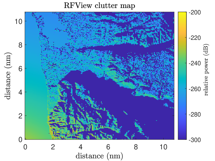
As an illustrative example, consider an airborne radar looking down on a heterogeneous terrain, consisting of mountains, water bodies, and foliage simulated by RFView as shown in Fig.1. Fig.1 displays the relative power of the returned signal from such heterogeneous terrain in Southern California near San Diego. We observe that the regions of high-power returns have less area compared to the regions of low-power return, with noise power higher than the low-power returns. This is evident from the eigenvalue plot of the clutter plus noise covariance matrix in Fig. 2, computed from the return signal. A large number of eigenvalues of the clutter covariance matrix fall below the noise power.

In this paper, we use a nonlinear shrinkage-based rotation invariant estimator developed in [3] to estimate the clutter plus noise covariance matrix in a high dimensional setting. In the spiked covariance model, we only need to estimate the noise power and the spiked components.
We show that for the estimation of covariance matrix of dimension , the proposed algorithm performs real-valued multiplications for the joint noise power-clutter rank estimation as compared to the in the RCML-EL11 1 RCML-ELrepresents the RCML covariance estimator [6] with the clutter rank and noise power obtained by the expected likelihood (EL) approach [7]. algorithm with identical SCNR and error variance. Additionally, we state the convergence results for the estimated eigenvalues and bounds for normalized SCNR for the proposed estimator. We test the target detection performance of the estimator using Low-Rank Adaptive Normalized Matched Filter (LR-ANMF) detector. We empirically show the robustness of the detector against contaminating clutter discretes. We apply the proposed algorithm on the Challenge Dataset simulated by RFView software.
I-A Related Works
The problem of covariance matrix estimation, [8], with data deficient scenario has received considerable attention in the radar signal processing literature. In the data deficient scenarios, the sample covariance matrix is no longer a reliable estimator as it becomes ill-conditioned. To address such ill-conditioning, methods like diagonal loading [9, 10, 11, 12, 13, 14, 15] and factored space-time approaches [16] have been proposed. Data dependent techniques include Principal Components Inverse [17], Multistage Wiener Filter [18], Parametric Adaptive Matched Filter [19], and EigenCanceler [20]. Data independent approaches include JDL-GLR [21].
In a high-dimensional setting, the properties of covariance matrices are explained by the Random Matrix Theory as stated in [22, 23, 24, 25]. In such high dimensional settings, shrinkage estimators have been developed to estimate covariance matrices in signal processing and finance. Shrinkage estimators have been used in wireless communications [26] to estimate the channel matrices, in array signal processing to estimate direction of arrival [27] and in finance for Markowitz Portfolio optimization [28, 29, 30, 31]. Shrinkage methods include Ledoit-Wolf shrinkage estimator [32], regularized PCA [33], Ridge and Lasso shrinkage estimators [34] and regularized M-estimators [35].
In radar signal processing, the covariance matrices often contains a low-rank structure corresponding to the clutter. The covariance matrices are called clutter plus noise covariance matrices. Covariance estimation algorithms developed in [36, 37, 7, 38, 39], propose estimation schemes assuming a rank sparse clutter covariance matrix in a high dimensional setting. These papers use Brennan’s Rule which gives an estimate of the rank depending on the dominant components of the clutter and the jammers. However, as demonstrated in [40, 41, 42], Brennan’s rule fails when a plethora of real-world effects such as internal clutter motion, mutual coupling between antenna array elements arise on account of the system and environmental factors. In our paper, the data generated from the high fidelity, site-specific, physics-based, radar scenario simulation software RFview is used where the Brennan rule does not prevail as documented in [4].
To address these issues we exploit the spiked covariance structure, as proposed in [1, 2, 43, 44], of the clutter plus noise covariance matrix. We use the nonlinear shrinkage estimation techniques of [3] to estimate the covariance matrix. Spiked covariance models have been used to estimate direction of arrival (DOA) in array signal processing, as demonstrated in [45], and for target detection in [46]. We are using the spiked covariance model to estimate the clutter plus noise covariance matrix.
I-B Main Results and Organization
The main results and organization of this paper are as follows:
- 1.
- 2.
In Sec. III, we present the algorithm proposed in [3] for spiked covariance matrix estimation. In Sec. III-III-A, Theorem 1 shows a strong law of large numbers (namely, the estimated spiked eigenvalues converge almost surely to a constant) and satisfy a Central Limit Theorem. This is due to the fact that, even though we are in a high-dimensional setting, the number of spikes are constant. Empirical verification of the convergence properties for RFview Challenge Dataset is provided. We derive the bounds for normalized SCNR, , in Sec. III-III-B. In Sec. III-III-C, we establish that the proposed algorithm and the RCML-EL estimation algorithm in high dimensions have similar performance due to the fact they share a common optimization problem. In Sec. III-III-D, we employ the LR-ANMF detector for target detection when using a rotation invariant estimator.
- 3.
In Sec. IV-IV-A, we demonstrate that the proposed algorithm has identical SCNR compared to the RCML-EL algorithm for the Challenge Dataset simulated using RFView. We further show that the computation time of estimation by the proposed algorithm is less than that of the RCML-EL algorithm. In Sec. IV-IV-B, we compute the target detection probabilities for various false alarm probabilities and SCNR and empirically show its robustness with respect to contaminating clutter discretes. In Sec. IV-IV-C, we compute the error variance of the MVDR beamformer for the proposed algorithm.
II Rotation Invariant Estimator and Spiked Covariance Model
This section is organized as follows. Sec. II-II-A presents a general rotation invariant estimator. Sec. II-II-B describes the high-dimensional spiked covariance model.
We use a narrowband baseband equivalent model used in [4]. The radar transmits a complex-valued waveform and receives a complex-valued return in discrete time:
| (1) |
Here is the convolution operator and denotes discrete time. is the complex valued target impulse response and is the complex valued clutter impulse response. The noisy measurement is the additive white Gaussian noise with variance with zero mean. The noise samples are independent, identically, distributed (i.i.d).
In matrix-vector notation (1) reads
| (2) |
where are Toeplitz matrices constructed by the impulse responses and , respectively. is return signal of length and is the waveform of pulse length . The noise is a complex valued Gaussian distributed vector where and has i.i.d samples.
We define the clutter plus noise return as
| (3) |
II-A Rotation Invariant Estimator
In this subsection, we describe the rotation invariant estimation for the clutter plus noise covariance estimator. Rotation invariant estimators have the same eigenvectors as that of the sample covariance matrix and the eigenvalues of the estimators are a function of the eigenvalues of the sample covariance matrix.
The clutter plus noise covariance matrix is given by
| (4) |
where the clutter covariance matrix is
| (5) |
and is the noise component. The eigendecomposition of clutter plus noise covariance is:
| (6) |
with eigenvalues and eigenvectors . The sample covariance matrix is:
| (7) |
where is the clutter plus noise return defined in (3) which will be used as training data samples22 2 The training data is collected by RFView when no target is present. We assume that the clutter plus noise covariance matrix is stationary and is independent of the target presence. This is due to the fact that eigenvalue component due to the target is independent of the eigenvalues of the clutter plus noise covariance matrix in the spiked covariance model which is defined in Sec. II-II-B., is the discrete time and are the number of training data samples. The spectral decomposition of for a given training data size is:
| (8) |
where are the eigenvalues and are the eigenvectors of . The spiked covariance matrix estimate for a given number of data samples is:
| (9) |
where are the eigenvalues of , with eigenvectors identical to those of the in (8). The spiked covariance estimator is a rotation invariant estimator.
Additionally, we use normalized SCNR to compare covariance estimation methods. We denote to define the normalized SCNR as:
| (10) |
where is the Kronecker product of angle steering vector and the Doppler steering vector . and are defined in Sec. IV. The dimension of the covariance matrix is .
In the next section, we will show that is a nonlinear function of , where the nonlinearity depends on the loss function.
II-B Clutter Plus Noise Covariance Matrix Modelling using Large Random Matrices
In this subsection, we define the spiked covariance model and the asymptotic regime for the high dimensional setting. We use this framework to model the clutter plus noise covariance matrix.
Definition 1
A spiked covariance matrix is a positive definite Hermitian matrix with eigenvalues such that for a finite , and .
We make two assumptions
- 1.
- 2.
There exists a such that for given training data size with the dimension of the covariance matrix as such that:
(11)
Data displayed in Fig. 1 and Fig. 2 satisfies these conditions. In Fig. 2, we see that the clutter covariance matrix can be approximated by a rank positive semi-definite matrix as the remaining components are below the noise floor.
We assume that clutter plus noise covariance matrix is spiked if the rank of the clutter matrix is less than a fraction of the clutter plus noise covariance matrix. For convenience, we choose , since it empirically fits with the data simulated by RFView. A more general approach involves model order (dimension) estimation. In the classical statistical setting, this is well studied in terms of penalized likelihood methods such as Akaike Information Criterion (AIC) [47], Minimum Description Length (MDL) [48], information theoretic criteria [49], statistical techniques [50], data dependent techniques [51], and min-max approaches such as the Embedded Exponential Families [52]. However, in the high dimensional setting considered in this paper, estimating the model order (number of spikes) is a difficult problem not addressed in this paper. In [7], the RCML-EL algorithm uses Brennan’s rule, [8], as an initial estimate for the rank of the clutter covariance matrix to determine the model order. RCML-EL algorithm correctly estimates the rank as compared to the AIC and MDL techniques. In Sec. III-III-C, since the proposed algorithm and RCML-EL algorithm share similar optimization problem, the proposed algorithm correctly estimates the model order.
The spiked covariance property helps us to deal with the clutter plus noise covariance matrices in high dimensions, which is frequently encountered in radar signal processing. With this knowledge, we define the nonlinear shrinkage-based rotation invariant estimator.
III Nonlinear Shrinkage Estimation
In this section, we propose the rotation invariant estimator using nonlinear shrinkage of the eigenvalues of the sample covariance matrix. We state the convergence of the estimated eigenvalues in Theorem 1 in Sec. III-III-A. It is to be noted that we use the terms spiked eigenvalues and the leading eigenvalues of the covariance matrix interchangeably for a fixed clutter covariance matrix with rank . We outline the computation cost of the proposed algorithm. We propose bounds for the normalized SCNR() in Sec. III-III-B. We show the similarity of SCNR performance between the proposed algorithm and the RCML-EL algorithm in high dimensions in Sec. III-III-C. We conclude this section by stating the Adaptive Normalized Matched Filter for target detection for the proposed algorithm in Sec. III-III-D.
The spiked covariance matrix is stated in Definition 1. Estimation of the spiked covariance matrix as defined in (9), consists of two sub-problems: estimation of the spiked eigenvalues and the estimation of the noise power .
- 1.
The estimate of the noise power is given as stated in [3] is
(12) where is the median of the eigenvalues of the sample covariance matrix and is the median of the Marchenko-Pastur distribution with parameter stated in (11). The proof of the consistency of the noise power estimator is given in [3, Sec. 9].
- 2.
The shrinkage function as stated in [3] is
(13) where , are the eigenvalues of the sample covariance matrix and is defined in (12). The function given by
and for Stein loss as stated in [3], , is given by
(16) where is given by
(17) and is given in (11).
The eigenvalues of the estimator are given by:(18) where is given in (12) and is given in (13). The proof of optimality of this estimator is given in [3, Sec. 6].
A pseudo-code to compute the estimator is stated in Algorithm 1.
III-A Convergence of Eigenvalues of the Proposed Estimator
Although we are dealing with finite and , in Theorem 1 we state that the spiked eigenvalues converge almost surely to a constant and satisfy a Central Limit Theorem when both , given that the number of spikes is fixed.
We assume the following for a covariance matrix with dimension :
- A1.
Leading distinct eigenvalues with multiplicity 1 and lower bounded by .
- A2.
Eigenvalues .
Theorem 1
Proof: Almost sure convergence can be proved by applying Continuous Mapping Theorem on [2, Thm. 2] with function . The in-distribution convergence can be proved by applying the delta method on [2, Thm. 3] with function .
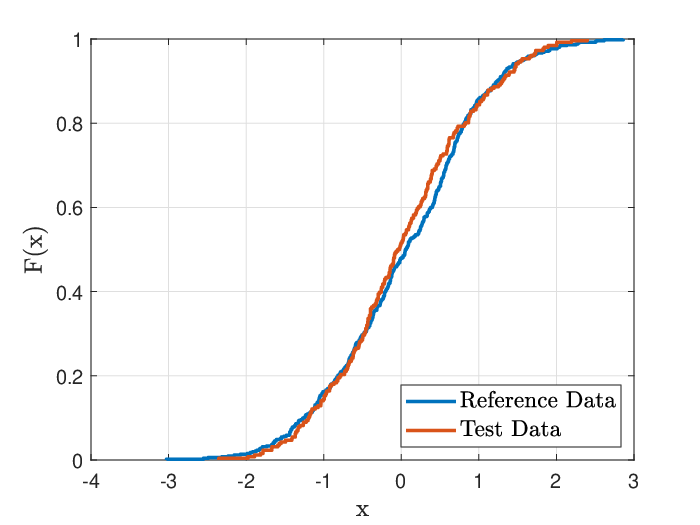
We empirically showed the validity of assumptions of Theorem 1 for the Challenge Dataset using the double version of the Kolmogorov-Smirnov (K-S) test with significance level and 1024 Monte Carlo simulations. The reference data was generated from the prescribed distribution in (20) and the test data was generated from the Challenge Dataset. The CDF plot in Fig.3 for the test and reference data reveals that the Challenge Dataset satisfies the assumptions for Theorem 1.
Computation Cost
Algorithm 1 does not require prior knowledge of the number of spikes. Step (2) and Step (3) in Algorithm 1 determine the eigenvalues that are above the noise floor. The computation cost of the algorithm is given below:
- 1.
The eigenvalue decomposition requires real-valued multiplications.
- 2.
The noise power estimation, step (2), is a median finding algorithm that requires real-valued multiplications.
- 3.
The nonlinear shrinkage, step (3), requires real-valued multiplications, being the rank of the clutter covariance matrix.
We compare algorithm 1 to the RCML-EL algorithm whose computational cost is given as follows:
- 1.
The eigenvalue decomposition step takes real valued multiplications.
- 2.
The joint noise and rank estimation step takes real valued multiplications.
The difference is in the noise and rank estimation step; Algorithm 1 takes real-valued multiplications and the RCML-EL algorithm takes . This will be demonstrated in Sec. IV-IV-A empirically.
III-B Bounds for
In this section, we derive the lower and upper bounds for the normalized SCNR() using results from [53].
We rewrite from (10)
| (21) |
where . Without loss of generality, assume . We use the matrix version of Kantorovich’s inequality to bound the denominator. For a positive semi-definite matrix, A, and a unit vector x, , where is the condition number of the matrix . By Cauchy-Schwartz Inequality . We lower bound by:
| (22) |
where . From [53], we have
| (23) |
where
defined in (16) and .
In Sec. IV we shall demonstrate that the proposed algorithm performs within the derived bounds.
III-C Performance similarity between Proposed Algorithm and RCML-EL Algorithm
In this section, we show that the proposed algorithm and the RCML-EL algorithm will give similar SCNR performance.
The optimization problem for clutter plus noise covariance matrix estimation assuming noise power to be unity defined in [6, (35)] is:
| (24) | ||||
where , recall from Sec. II that is eigenvalue of the estimator and is the eigenvalue of the sample covariance matrix.
,
The first constraint in (24) enforces to be positive in descending order and the second constraint enforces the last eigenvalues of the estimator to be equal. These constraints enforce a spiked covariance matrix structure on the estimator, stated in Definition 1, in a high dimensional setting. In [3], the optimization problem for estimating leading eigenvalues for Stein loss under a spiked covariance model is given by:
| (25) |
where , and ; is given in (2), is given in (15), and are given in (17).
Since the cost function of (24) is identical to (25) within a constant and the constraints of (24) are implicit to the optimization problem of (25), the normalized SCNR, and the rank of the clutter covariance matrix, , will be identical.
In Sec. IV we shall demonstrate that the SCNR performance for the proposed algorithm is identical to the RCML-EL algorithm with a reduced computation time.
III-D Low-Rank Adaptive Normalized Matched Filter Detection
In this section, we shall use the Low-Rank Adaptive Normalized Matched Filter (LR-ANMF) detector for a rotation-invariant estimator as stated in [54]. This detection scheme is independent of the eigenvalue shrinkage in (13) and only depends on the eigenvectors of the sample covariance matrix in high dimensions. This detector is the same for both the proposed algorithm and the RCML-EL algorithm.
We have the following binary hypothesis for a single target:
| (26) | ||||
where is the null hypothesis when no target is present and is the alternate hypothesis when the target is present. The target signal is defined in the same way as in (10) with a complex-valued amplitude and is the clutter plus noise covariance matrix. The test statistics for the LR-ANMF with data samples, as stated in [55], is
| (27) |
where
is a projection matrix constructed using the eigenvectors defined in (8) corresponding to the spikes of the spiked covariance matrix and is the detection threshold. Recall from Sec. II-II-B that is the rank of the clutter covariance matrix. The knowledge of noise power is not impacting the detection since we are using assumption (A1) in Sec. III-III-A where has already been estimated. We present the convergence theorems from [54] that state the in-distribution convergence of the test statistics under and .
Theorem 2 ([54], Thm 2)
Under and assumption (A1) the test statistics satisfies:
| (28) |
where is a chi-squared distribution with one complex degree of freedom. The probability of false alarm with detection threshold is:
| (29) |
Theorem 3 ([54], Thm 3)
Under and assumption (A1) the test statistics satisfies:
| (30) |
where denotes the cumulative distribution of a non-central distribution with one complex degree of freedom and non-centrality parameter .
| (31) |
is defined in (26),
where , is defined in (17), defined in (6), is rank of the clutter covariance matrix and defined in (26). The corresponding target detection probability with detection threshold is:
| (32) | ||||
where is the gamma function.
In Sec. IV-IV-B, we compute the detection probabilities for different false alarm probabilities over a range of signal-to-noise ratios (SNR), we empirically evaluate the robustness of the detector for detecting a single target in the presence of multiple targets that act as contaminating clutter discretes. Contaminating clutter discretes are additional spikes that are present due to undesired targets. They are not part of clutter spikes and change the clutter covariance matrix rank from to .
To conclude this section, we proposed the nonlinear shrinkage-based rotation invariant estimator by using the sample covariance matrix. We stated the convergence of the spiked eigenvalues of the estimator. We stated the bounds for the normalized SCNR. The equivalence of the RCML-EL algorithm in a high dimensional setting to the proposed algorithm was established. A detector for target detection was stated for the proposed algorithm.
IV NUMERICAL EXAMPLES
We use a dataset generated using software that provides an accurate characterization of complex RF environments. It uses stochastic transfer functions [4] to simulate the high-fidelity RF clutter encountered in practice.
The dataset consists of a data cube in the time domain and is a multi-dimensional matrix, where is the total number of (fast-time), is the slow time and is the number of range gates in a specified coherent processing interval. For our case, we use the range gates as the number of data samples .
In Sec. IV-IV-A, we use the Challenge Dataset generated by RFView. We compare the performance of the Algorithm 1 against the RCML-EL based estimation algorithm given in [7]. We plot the normalized SCNR (), stated in (10), as a function of training data size , the normalized Doppler, and the normalized angle. For all the plots we are simulating in the regime where , i.e., . We also demonstrate the computation times for our proposed algorithm and the RCML-EL algorithm for various .
In Sec. IV-IV-B, we compute the target detection probabilities over a range of false alarm probabilities and SCNR. In Sec. IV-IV-C, we compute the error variance of the minimum variance distortionless response beamformer using the proposed algorithm and compare it with the error variance corresponding to the RCML-EL algorithm and the true covariance matrix.
We only compare with the RCML-EL algorithm because it outperforms the Sample covariance matrix SMI, FML [56], Chen’s algorithm [57] and AIC [47], as documented in [7] in all metrics. Since the theory underlying Theorem 1 holds only in the regime of , no definitive statements can be made for the case of . Therefore, the validity of the proposed algorithm is restricted to the case of .
We simulated our results -R2021b on Windows-11 OS running on AMD Ryzen 7 5800H microprocessor with 16GB RAM.
IV-A SCNR Performance
The Challenge dataset contains radar target and clutter returns generated by . The scenario in Challenge Dataset has 4 targets and ground clutter containing buildings. This scenario involves an airborne monostatic radar flying over the Pacific Ocean near the coast of San Diego looking down for ground moving targets. The data spans several coherent processing intervals as the platform is moving with constant velocity along the coastline. In Table II-IX, Appendix we state all the parameters used for this scenario.
The data set consists of a data cube matrix which has the clutter impulse response over 32 channels with 64 pulses and 2335 data samples. We concatenate channels to get a clutter impulse response matrix of size . We convolve the rows of the clutter impulse response matrix with a waveform of pulse length to get a clutter return matrix of dimension . We add additive white Gaussian noise with zero-mean and variance to the resulting clutter return matrix. The dimension of the clutter plus noise covariance matrix is . We vary in the multiples of till to get the sample covariance matrix. For each plot, we use 1024 Monte Carlo simulations. For normalized Doppler, we fix the angle interval at and marginalize over it. For the normalized angle, we fix the Doppler interval at and marginalize over it. For both cases, we fix .
Fig. 4 displays the average normalized SCNR vs. the number of data samples . The run-time for different is given in Table I. Normalized SCNR vs. normalized Doppler is given in Fig. 5 and normalized SCNR vs. normalized angle in Fig. 6.
| Training Data Size () | Proposed Algorithm | RCML-EL algorithm |
|---|---|---|
| 512 | 0.012035s | 0.107116s |
| 1024 | 0.003046s | 0.070876s |
| 1536 | 0.002028s | 0.053037s |
| 2048 | 0.002026s | 0.050819s |
| 2560 | 0.002095s | 0.050504s |


IV-B Target Detection
In this section, we use results from Sec. III-III-D with the target having a Doppler of and an angle of . We plot the target detection probability as we vary false alarm probability from to in the multiples of 10 from SCNR=-10dB to 30dB. We use data samples with 1024 Monte Carlo Simulations.
The Challenge Dataset contains 4 targets. We consider detecting a single target with remaining targets constituting contaminating clutter discretes. These contaminating clutter discretes do not share the same characteristics as the target of interest so there is no self-target cancellation. Recall from Sec. III-III-D that the contaminating clutter discretes change the clutter rank to an unknown . By introducing multiple targets as contaminating clutter discretes we demonstrate the robustness of the detector.
The detection probabilities are the same for both the RCML-EL algorithm and the proposed algorithm as the detector uses only the eigenvectors of the sample covariance matrix. The detection probabilities are illustrated in Fig.7.

IV-C Empirical Error Variance
In this section, we empirically present the minimum variance distortionless beamformer (MVDR) error variance due to the proposed algorithm with the error variance of the beamformer of the RCML-EL algorithm and the true covariance matrix. The error variance for the beamformer is
| (33) |
where for the proposed algorithm, for the RCML-EL algorithm and for the true covariance matrix, respectively. The target signal , as defined like in (10), has Doppler and angle . In Fig.8, the error variance for RCML-EL and the proposed algorithm is identical to the true covariance matrix. The error variance does not change as the training data size is increased since we are working in the asymptotic regime. This is due to the fact that in the asymptotic regime, the estimated covariance matrix converges to the true covariance matrix with probability 1. Hence, the error variance in (33) merely becomes the reciprocal of the SNR from (10) when .

To conclude this section, we demonstrated that with reduced covariance computation time, Algorithm 1 gives identical SCNR performance compared to the EL-based covariance estimation algorithm within the proposed bounds. However, the noise computation step requires some pre-computed values of the medians of Marchenko Pastur distributions for various values of . This also makes our algorithm less robust to a sudden change in the parameters of the scenario as data samples can vary depending on the range swath.
We demonstrated the target detection probabilities for different false alarm probabilities using the LR-ANMF detector. We empirically demonstrated the robustness with respect to contaminating clutter discretes in the Challenge Dataset. We empirically demonstrated that the error variance of the proposed algorithm is identical to the true covariance matrix.
CONCLUSION
We exploited the spiked covariance structure for the clutter plus noise covariance matrix in a high dimensional setting and proposed a nonlinear shrinkage-based rotation invariant estimator. We stated the convergence of the spiked eigenvalues of the estimator. We demonstrated the reduced covariance computation times compared to the RCML-EL algorithm. Our proposed algorithm had identical SCNR performance compared to the RCML-EL algorithm. We employed the LR-ANMF detector for robust target detection and empirically showed that the error variance of the algorithm is identical to the true covariance matrix.
Our proposed algorithm is a batch-wise algorithm. In future work it is worthwhile developing an adaptive version of the algorithm. We will also investigate other kinds of loss functions for various scenarios by introducing various constraints and deriving the concentration bounds for the proposed algorithm. The number of contaminating clutter discretes and their relative strength in the challenge dataset is not sufficient to provide a comprehensive analysis of the robustness feature of the LR-ANMF detector. This facet of the technique will be explored in more detail in the future.
Appendix A Challenge Dataset Parameters

| Latitude | 32.66 deg. N |
|---|---|
| Longitude | 118 deg. W |
| Height | 6000 m |
| Speed | 100 m/s |
| Azimuth angle of velocity vector (deg. w.r.t. true north) | 0 deg |
| Elevation angle of velocity vector (deg. w.r.t. horizon) | 0 deg |
| Number of Array Elements (Horizontal Dimension) | 32 |
| Number of Array Elements (Vertical Dimension) | 5 |
| Number of Horizontal Spatial Channels (Receiver) | 32 |
| Number of Vertical Spatial Channels (Receiver) | 1 |
| Total Number of Spatial Channels (Receiver) | 32 |
| Total Number of Channels (Transmitter) | 1 |
| Transmit Antenna Gain | 503.3509 |
| Receive Antenna Gain | 15.7297 |
| Center Frequency | 10 GHz |
| Array Inter-Element Spacing | 0.015 m |
| Number of Coherent Processing Intervals (CPI) | 30 |
| Number of Pulses per CPI | 64 |
| Pulse Repetition Frequency | 1 KHz |
| Radar Waveform | Standard LFM |
| Radar Waveform Bandwidth | 10 MHz |
| Radar Waveform Duty Factor | 0.1 |
| Sampling Frequency | 10000000 |
| Peak Transmit Signal Power | 1000 Watts |
| Number of Range Bins | 2334 |
| Size of Data Cubes (for each CPI) | 32 x 64 x 2334 |
| Range Swath Width | 20000 m |
| Radar Azimuth Look Angle (Fixed) | 80.8321 deg |
| Radar Elevation Look Angle (Fixed) | -5.1364 deg |
| Clutter Scene Size | 20Km x 20Km |
| Clutter Patch Size | 20m x 20m |
| Latitude | 32.7627 deg. N |
|---|---|
| Longitude | 117.2524 deg. W |
| Height | 0 m |
| Speed | 10 m/s |
| Azimuth angle of velocity vector (deg. w.r.t. true north) | 0 |
| Elevation angle of velocity vector (deg. w.r.t. horizon) | 0 |
| RCS | 40 |
| Latitude | 32.7668 deg. N |
|---|---|
| Longitude | 117.2334 deg. W |
| Height | 0 m |
| Speed | 20 m/s |
| Azimuth angle of velocity vector (deg. w.r.t. true north) | 0 |
| Elevation angle of velocity vector (deg. w.r.t. horizon) | 0 |
| RCS | 40 |
| Latitude | 32.793 deg. N |
|---|---|
| Longitude | 117.283 deg. W |
| Height | 0 m |
| Speed | 10 m/s |
| Azimuth angle of velocity vector (deg. w.r.t. true north) | 180 |
| Elevation angle of velocity vector (deg. w.r.t. horizon) | 0 |
| RCS | 20 |
| Latitude | 32.763 deg. N |
|---|---|
| Longitude | 117.283 deg. W |
| Height | 0 m |
| Speed | 15 m/s |
| Azimuth angle of velocity vector (deg. w.r.t. true north) | 0 |
| Elevation angle of velocity vector (deg. w.r.t. horizon) | 0 |
| RCS | 30 |
| Latitude | 32.7665 deg. N |
|---|---|
| Longitude | 117.2305 deg. W |
| Height | 6 m |
| Speed | 0 m/s |
| RCS | 50 |
| Latitude | 32.7901 deg. N |
|---|---|
| Longitude | 117.252 deg. W |
| Height | 6 m |
| Speed | 0 m/s |
| RCS | 50 |
References
- [1] I. M. Johnstone, “On the distribution of the largest eigenvalue in principal components analysis,” The Annals of statistics, vol. 29, no. 2, pp. 295–327, 2001.
- [2] D. Paul, “Asymptotics of sample eigenstructure for a large dimensional spiked covariance model,” Statistica Sinica, pp. 1617–1642, 2007.
- [3] D. L. Donoho, M. Gavish, and I. M. Johnstone, “Optimal shrinkage of eigenvalues in the spiked covariance model,” Annals of statistics, vol. 46, no. 4, p. 1742, 2018.
- [4] S. Gogineni, J. R. Guerci, H. K. Nguyen, J. S. Bergin, D. R. Kirk, B. C. Watson, and M. Rangaswamy, “High fidelity rf clutter modeling and simulation,” IEEE Aerospace and Electronic Systems Magazine, vol. 37, pp. 24–43, November 2022.
- [5] https://rfview.islinc.com/RFView/login.jsp. Accessed: 2022-12-02.
- [6] B. Kang, V. Monga, and M. Rangaswamy, “Rank-constrained maximum likelihood estimation of structured covariance matrices,” IEEE Transactions on Aerospace and Electronic Systems, vol. 50, no. 1, pp. 501–515, 2014.
- [7] B. Kang, V. Monga, M. Rangaswamy, and Y. Abramovich, “Expected likelihood approach for determining constraints in covariance estimation,” IEEE Transactions on Aerospace and Electronic Systems, vol. 52, no. 5, pp. 2139–2156, 2016.
- [8] I. Reed, J. Mallett, and L. Brennan, “Rapid convergence rate in adaptive arrays,” IEEE Transactions on Aerospace and Electronic Systems, vol. AES-10, no. 6, pp. 853–863, 1974.
- [9] Y. I. Abramovich and A. Nevrev, “An analysis of effectiveness of adaptive maximization of the signal-to-noise ratio which utilizes the inversion of the estimated correlation matrix,” Radio Engineering and Electronic Physics, vol. 26, no. 12, pp. 67–74, 1981.
- [10] B. A. Johnson and Y. I. Abramovich, “A matrix extension built under-sampled likelihood ratio test with application to music breakdown prediction and cure.,” J. Commun., vol. 2, no. 3, pp. 64–72, 2007.
- [11] Y. I. Abramovich, “A controlled method for adaptive optimization of filters using the criterion of maximum signal-to-noise ratio,” Radio Eng. Elect. Phys, vol. 26, no. 3, pp. 87–95, 1981.
- [12] B. D. Carlson, “Covariance matrix estimation errors and diagonal loading in adaptive arrays,” IEEE Transactions on Aerospace and Electronic systems, vol. 24, no. 4, pp. 397–401, 1988.
- [13] M. C. Wicks, M. Rangaswamy, R. Adve, and T. B. Hale, “Space-time adaptive processing: a knowledge-based perspective for airborne radar,” IEEE Signal Processing Magazine, vol. 23, no. 1, pp. 51–65, 2006.
- [14] F. Gini and M. Rangaswamy, Knowledge based radar detection, tracking and classification. John Wiley & Sons, 2008.
- [15] J. Ward, “Space time adaptive processing,” Technical Report ESC-TR, pp. 94–109, 1994.
- [16] R. C. DiPietro, “Extended factored space-time processing for airborne radar systems,” in Conference Record of the Twenty-Sixth Asilomar Conference on Signals, Systems & Computers, pp. 425–426, IEEE Computer Society, 1992.
- [17] I. P. Kirsteins and D. W. Tufts, “Adaptive detection using low rank approximation to a data matrix,” IEEE Transactions on Aerospace and Electronic Systems, vol. 30, no. 1, pp. 55–67, 1994.
- [18] J. S. Goldstein, I. S. Reed, and L. L. Scharf, “A multistage representation of the wiener filter based on orthogonal projections,” IEEE Transactions on Information Theory, vol. 44, no. 7, pp. 2943–2959, 1998.
- [19] J. R. Roman, M. Rangaswamy, D. W. Davis, Q. Zhang, B. Himed, and J. H. Michels, “Parametric adaptive matched filter for airborne radar applications,” IEEE Transactions on Aerospace and Electronic Systems, vol. 36, no. 2, pp. 677–692, 2000.
- [20] A. Haimovich, “The eigencanceler: Adaptive radar by eigenanalysis methods,” IEEE Transactions on Aerospace and Electronic Systems, vol. 32, no. 2, pp. 532–542, 1996.
- [21] H. Wang and L. Cai, “On adaptive spatial-temporal processing for airborne surveillance radar systems,” IEEE Transactions on aerospace and electronic systems, vol. 30, no. 3, pp. 660–670, 1994.
- [22] M. J. Wainwright, High-dimensional statistics: A non-asymptotic viewpoint, vol. 48. Cambridge University Press, 2019.
- [23] R. Vershynin, High-dimensional probability: An introduction with applications in data science, vol. 47. Cambridge university press, 2018.
- [24] Z. Bai and J. W. Silverstein, Spectral analysis of large dimensional random matrices, vol. 20. Springer, 2010.
- [25] W. Wang and J. Fan, “Asymptotics of empirical eigenstructure for high dimensional spiked covariance,” Annals of statistics, vol. 45, no. 3, p. 1342, 2017.
- [26] A. M. Tulino, S. Verdú, et al., “Random matrix theory and wireless communications,” Foundations and Trends® in Communications and Information Theory, vol. 1, no. 1, pp. 1–182, 2004.
- [27] R. Couillet, F. Pascal, and J. W. Silverstein, “A joint robust estimation and random matrix framework with application to array processing,” in 2013 IEEE International Conference on Acoustics, Speech and Signal Processing, pp. 6561–6565, IEEE, 2013.
- [28] O. Ledoit and M. Wolf, “Optimal estimation of a large-dimensional covariance matrix under stein’s loss,” Bernoulli, vol. 24, no. 4B, pp. 3791–3832, 2018.
- [29] O. Ledoit and M. Wolf, “Quadratic shrinkage for large covariance matrices,” Bernoulli, vol. 28, no. 3, pp. 1519–1547, 2022.
- [30] O. Ledoit and M. Wolf, “Nonlinear shrinkage of the covariance matrix for portfolio selection: Markowitz meets goldilocks,” The Review of Financial Studies, vol. 30, no. 12, pp. 4349–4388, 2017.
- [31] O. Ledoit and M. Wolf, “The power of (non-) linear shrinking: A review and guide to covariance matrix estimation,” Journal of Financial Econometrics, vol. 20, no. 1, pp. 187–218, 2022.
- [32] O. Ledoit and M. Wolf, “A well-conditioned estimator for large-dimensional covariance matrices,” Journal of multivariate analysis, vol. 88, no. 2, pp. 365–411, 2004.
- [33] J. Bun, R. Allez, J.-P. Bouchaud, and M. Potters, “Rotational invariant estimator for general noisy matrices,” IEEE Transactions on Information Theory, vol. 62, no. 12, pp. 7475–7490, 2016.
- [34] X. Yuan, W. Yu, Z. Yin, and G. Wang, “Improved large dynamic covariance matrix estimation with graphical lasso and its application in portfolio selection,” IEEE Access, vol. 8, pp. 189179–189188, 2020.
- [35] R. Couillet, F. Pascal, and J. W. Silverstein, “Robust estimates of covariance matrices in the large dimensional regime,” IEEE Transactions on Information Theory, vol. 60, no. 11, pp. 7269–7278, 2014.
- [36] S. Sen, “Low-rank matrix decomposition and spatio-temporal sparse recovery for stap radar,” IEEE Journal of Selected Topics in Signal Processing, vol. 9, no. 8, pp. 1510–1523, 2015.
- [37] K. Duan, H. Yuan, H. Xu, W. Liu, and Y. Wang, “Sparsity-based non-stationary clutter suppression technique for airborne radar,” IEEE Access, vol. 6, pp. 56162–56169, 2018.
- [38] B. Kang, V. Monga, and M. Rangaswamy, “Constrained ml estimation of structured covariance matrices with applications in radar stap,” in 2013 5th IEEE International Workshop on Computational Advances in Multi-Sensor Adaptive Processing (CAMSAP), pp. 101–104, IEEE, 2013.
- [39] R. Abrahamsson, Y. Selen, and P. Stoica, “Enhanced covariance matrix estimators in adaptive beamforming,” in 2007 IEEE International Conference on Acoustics, Speech and Signal Processing-ICASSP’07, vol. 2, pp. II–969, IEEE, 2007.
- [40] J. R. Guerci, “Cognitive radar: A knowledge-aided fully adaptive approach,” in 2010 IEEE Radar Conference, pp. 1365–1370, IEEE, 2010.
- [41] B. Kang, S. Gogineni, M. Rangaswamy, J. R. Guerci, and E. Blasch, “Adaptive channel estimation for cognitive fully adaptive radar,” IET Radar, Sonar & Navigation, vol. 16, no. 4, pp. 720–734, 2022.
- [42] J. Guerci, J. Bergin, R. Guerci, M. Khanin, and M. Rangaswamy, “A new mimo clutter model for cognitive radar,” in 2016 IEEE Radar Conference (RadarConf), pp. 1–6, IEEE, 2016.
- [43] B. Nadler, “Finite sample approximation results for principal component analysis: A matrix perturbation approach,” 2008.
- [44] F. Benaych-Georges and R. R. Nadakuditi, “The eigenvalues and eigenvectors of finite, low rank perturbations of large random matrices,” Advances in Mathematics, vol. 227, no. 1, pp. 494–521, 2011.
- [45] L. Yang, M. R. McKay, and R. Couillet, “High-dimensional mvdr beamforming: Optimized solutions based on spiked random matrix models,” IEEE Transactions on Signal Processing, vol. 66, no. 7, pp. 1933–1947, 2018.
- [46] B. D. Robinson, R. Malinas, and A. O. Hero, “Space-time adaptive detection at low sample support,” IEEE Transactions on Signal Processing, vol. 69, pp. 2939–2954, 2021.
- [47] H. Akaike, “A new look at the statistical model identification,” IEEE transactions on automatic control, vol. 19, no. 6, pp. 716–723, 1974.
- [48] P. D. Grünwald, The minimum description length principle. MIT press, 2007.
- [49] M. Wax and T. Kailath, “Detection of signals by information theoretic criteria,” IEEE Transactions on acoustics, speech, and signal processing, vol. 33, no. 2, pp. 387–392, 1985.
- [50] Z.-D. Bai, P. R. Krishnaiah, and L.-C. Zhao, “On rates of convergence of efficient detection criteria in signal processing with white noise,” IEEE Transactions on Information Theory, vol. 35, no. 2, pp. 380–388, 1989.
- [51] A. A. Shah and D. W. Tufts, “Determination of the dimension of a signal subspace from short data records,” IEEE Transactions on Signal Processing, vol. 42, no. 9, pp. 2531–2535, 1994.
- [52] S. Kay, “Exponentially embedded families-new approaches to model order estimation,” IEEE Transactions on Aerospace and Electronic Systems, vol. 41, no. 1, pp. 333–345, 2005.
- [53] D. L. Donoho and B. Ghorbani, “Optimal covariance estimation for condition number loss in the spiked model,” arXiv preprint arXiv:1810.07403, 2018.
- [54] P. Vallet, G. Ginolhac, F. Pascal, and P. Forster, “An improved low rank detector in the high dimensional regime,” in ICASSP 2019-2019 IEEE International Conference on Acoustics, Speech and Signal Processing (ICASSP), pp. 5336–5340, IEEE, 2019.
- [55] M. Rangaswamy, F. C. Lin, and K. R. Gerlach, “Robust adaptive signal processing methods for heterogeneous radar clutter scenarios,” Signal Processing, vol. 84, no. 9, pp. 1653–1665, 2004.
- [56] M. Steiner and K. Gerlach, “Fast converging adaptive processor or a structured covariance matrix,” IEEE Transactions on Aerospace and Electronic Systems, vol. 36, no. 4, pp. 1115–1126, 2000.
- [57] P. Chen, M. C. Wicks, and R. Adve, “Development of a statistical procedure for detecting the number of signals in a radar measurement,” IEE Proceedings: Radar, Sonar and Navigation, vol. 148, no. 4, pp. 219–226, 2001.