Stellar Populations in the Central 0.5 pc of Our Galaxy III: The Dynamical Sub-structuresFacilities: Keck Observatory AstroPy (Astropy Collaboration et al. 2013), Matplotlib (Hunter 2007), SciPy (Eric et al. 2001–)
Abstract
We measure the 3D kinematic structures of the young stars within the central 0.5 parsec of our Galactic Center using the 10 m telescopes of the W. M. Keck Observatory over a time span of 25 years. Using high-precision measurements of positions on the sky, and proper motions and radial velocities from new observations and the literature, we constrain the orbital parameters for each young star. Our results show two statistically significant sub-structures: a clockwise stellar disk with 18 candidate stars, as has been proposed before, but with an improved disk membership; a second, almost edge-on plane of 10 candidate stars oriented East-West on the sky that includes at least one IRS 13 star. We estimate the eccentricity distribution of each sub-structure and find that the clockwise disk has <> = 0.39 and the edge-on plane has <> = 0.68. We also perform simulations of each disk/plane with incompleteness and spatially-variable extinction to search for asymmetry. Our results show that the clockwise stellar disk is consistent with a uniform azimuthal distribution within the disk. The edge-on plane has an asymmetry that cannot be explained by variable extinction or incompleteness in the field. The orientation, asymmetric stellar distribution, and high eccentricity of the edge-on plane members suggest that this structure may be a stream associated with the IRS 13 group. The complex dynamical structure of the young nuclear cluster indicates that the star formation process involved complex gas structures and dynamics and is inconsistent with a single massive gaseous disk.
Keywords:
astrometry - Galaxy: center - infrared: stars - techniques: high angular resolutionI Introduction
Nuclear Star Clusters (NSCs) and Supermassive Black Holes (SMBHs) are found to coexist within the central parsec (pc) of many different types of galaxies (Graham & Spitler 2009). Furthermore, there are clear indications that NSCs, SMBHs, and their host galaxies evolve together. For example, Ferrarese et al. 2006 found that the relationship, the empirical correlation between the mass of the SMBH, , and the stellar velocity dispersion of the galaxy’s bulge, applies both for SMBHs and NSCs with similar slopes, although at a certain , NSCs are 10 times more massive than SMBHs. Additionally, Kormendy & Ho 2013 showed that the combined mass of the SMBH and NSC scales with a galaxy’s bulge mass with much less scatter than either the SMBH or the NSC separately, which suggests a strong dependency between their mutual formation and growth. The formation mechanism for NSCs is still widely debated as the strong tidal force at the Galactic Center will disrupt normal star formation.
Our own Galactic Center provides a unique test bed for understanding star formation around SMBHs since it harbors a population of around 200 young massive stars within 0.5 pc of the central SMBH, SgrA∗ (Genzel et al. 2000), including OB main-sequence stars, Wolf-Rayet (WR) stars, giants, and supergiants (Paumard et al. 2006; Bartko et al. 2010). Because the age of this population (Lu et al. 2013, 3 - 8 Myr) is much less than the relaxation timescale in the Galactic Center ( 1Gyr, Hopman & Alexander 2006), the origin of these stars can be constrained through studies of their dynamical structures. Only in the Galactic Center can we resolve individual stars and measure their motion, photometry, and spectroscopy with sufficient precision to constrain their dynamics and therefore constrain theories of star formation around SMBHs.
Observations of young stars at the Galactic Center currently favor in situ formation models, meaning that young stars are formed roughly where we see them today, within 0.5 pc of the SMBH (Paumard et al. 2006; Lu et al. 2009; Støstad et al. 2015). In situ formation is theoretically possible in an accretion disk around the SMBH, if it is massive enough to collapse vertically under its own self-gravity (Kolykhalov & Syunyaev 1980; Morris & Serabyn 1996; Sanders 1998; Goodman 2003; Levin & Beloborodov 2003; Nayakshin & Sunyaev 2005). When a disk reaches a surface density that is just large enough to initiate star formation, the first protostars form. Feedback from those stars will then heat the disk up to a point where it stabilizes against collapse and shuts off further disk fragmentation. In the meantime, those stars remain embedded in the disk and continue gaining mass at very high rates. As a result, an average star created in such a disk may become very massive. This process happens throughout the disk, from 0.01 pc to a few parsecs, with a peak effect at R 0.1 pc (Morris & Serabyn 1996; Vollmer & Duschl 2001; Nayakshin & Sunyaev 2005; Nayakshin 2006). This scenario can explain the existence of the disk of stars and the top-heavy Initial Mass Function (IMF) in our Galactic Center (Lu et al. 2013), although it may not be the only explanation.
However, if the disk is formed through steady accretion of gas, stars with circular orbits are more likely to form, which may contradict the observed eccentricity distribution that peaks at e=0.27 (Yelda et al. 2014). Furthermore, only 20% of the young stars are estimated to be in the disk and it is not clear whether 80% of the stars could be scattered from the disk in only 4 - 8 Myr. Modified in situ formation scenarios have been proposed, including: (a) the initial gas is not uniformly distributed, (b) stars form in repeated episodes, (c) after the gas disk collapses, the stars that form in it dynamically evolve off the disk. These formation scenarios can be disentangled by comparing the dynamical structures among different dynamical sub-groups. For example, if the initial gas is not uniformly distributed, we should see asymmetric sub-structures in their stellar systems.
Previous studies show that the young stars at the Galactic Center can be divided into three dynamical groups: (1) of the young stars (within 0.03 pc) are in the innermost region with high eccentricities and randomly oriented orbits. (2) of the young stars are on a well-defined clockwise (CW) rotating disk (0.03 - 0.5 pc) with moderate eccentricities . (3) of them are off-disk stars that extend over the same radius but have a more random distribution and eccentricity distribution with higher (Lu et al. 2013; Yelda et al. 2014). At smaller radii, dynamical effects will randomize the stellar orbits within 4-6 Myr, which is the case for the first group. The existence of the CW disk has already been verified to be significant () (Paumard et al. 2006; Bartko et al. 2010; Lu et al. 2009; Yelda et al. 2014). More recently, as many as 5 distinct sub-structures, including the CW disk, have been proposed by von Fellenberg et al. 2022. A detailed comparison between our result and previous work is presented in §VI.1 and Appendix B.
In this paper, we present improved dynamical measurements of the young stars at the Galactic Center derived from adaptive optics observations from the 10m Keck telescopes. We conduct novel simulations and comparative analyses of the properties of the different dynamical sub-groups of young stars within the central 0.5 pc of our Galaxy. The observational setup and data reduction are presented in Section II. Orbital parameters are derived in §III and the disk membership analysis is shown in §IV. Results of stellar disk properties and cluster simulations are presented in §V. We discuss our findings in §VI and summarize in §VII.
II Observations and Data Reduction
The kinematic analysis of the young stars at the Galactic Center requires both proper motion and radial velocity (RV) measurements in order to determine their orbital planes and disk membership probability. Details of the observations, data reduction, and image analysis are presented in Jia et al. 2019 and Do et al. 2009. Here, we briefly summarize the analysis methods most relevant to this work.
The photometry for those young stars is extracted from a deep, wide mosaic image (Lu et al. 2013). We applied the full extinction map from Schödel et al. 2010 to correct extinction with an average value of .
II.1 Sample Selection
In this work, we included all spectroscopically identified young (early-type) stars with well measured radial velocities (RV) and proper motions. To get a young star list with well-understood completeness, we combined new Galactic Center OSIRIS Wide-field Survey (GCOWS) observations (§II.2) with previous GCOWS observations (Do et al. 2013) and with other spectral types from the literature.
The GCOWS survey consists of observations with the Keck OSIRIS spectrograph behind the laser-guide-star adaptive optics system on the W. M. Keck Observatory (Larkin et al. 2006). We obtained diffraction-limited, medium spectral-resolution (R 4000) spectra with the Kn3 filter (2.121-2.220 ). We used two different plate scales: 35 mas in the central fields where the stellar densities are highest and 50 mas for the outer fields having relatively lower stellar density. Details on the GCOWS survey are presented by Do et al. 2009 and Do et al. 2013, who investigated young stars located in the central region and eastern field in the GC (green boxes in Figure 1). In this work, we have added new observations in the South and North (magenta boxes in Figure 1). The new spectroscopic observations are reported in Table 1. Data were reduced using the latest version of the OSIRIS data reduction pipeline (Lyke et al. 2017; Lockhart et al. 2019). This resulted in 7 more young stars with good quality RVs: S10-261, S10-48, S11-176, S11-21, S11-246, S12-76, S5- 106 (see §II.2 for reduction details). The sample of GCOWS stars used in this work includes those that are spectroscopically identified as early-type and that have sufficient Signal-to-Noise ratio (SNR) to measure a radial velocity (RV).
| Field Name | Field CenteraaR.A. and decl. offset from Sgr A* (R.A. offset is positive to the east). | Date | Scale | FWHMbbAverage FWHM of a relatively isolated star for the night, found from a two-dimensional Gaussian fit to the source. | Filter | PA | |
|---|---|---|---|---|---|---|---|
| (") | (UT) | (s) | (mas) | (mas) | (∘) | ||
| N5-3 | -0.37,11.21 | 2013-05-17 | 50 | 75 | Kn3 | 285 | |
| S4-1 | -0.87,-11.03 | 2014-05-20 | 50 | 90 | Kn3 | 195 | |
| S4-2 | -3.19,-10.41 | 2014-05-20 | 50 | 89 | Kn3 | 195 | |
| S4-3 | -5.50,-9.79 | 2014-06-05 | 50 | 140 | Kn3 | 195 | |
| S3-2 | -2.35,-7.31 | 2014-07-18 | 50 | 94 | Kn3 | 195 | |
| N5-1 | 4.40,9.93 | 2016-07-21 | 50 | 77 | Kn3 | 195 | |
| N5-1 | 4.40,9.93 | 2016-07-22 | 50 | 61 | Kn3 | 195 | |
| N5-2 | 2.01,10.58 | 2016-07-22 | 50 | 98 | Kn3 | 195 | |
| S2-3 | -3.80,-3.59 | 2019-05-25 | 50 | 89 | Kn3 | 195 | |
| S2-2 | -1.49,-4.21 | 2019-05-27 | 50 | 103 | Kn3 | 195 | |
| S3-1 | -0.03,-7.95 | 2019-05-27 | 50 | 135 | Kn3 | 195 | |
| S3-1 | -0.03,-7.95 | 2019-07-08 | 50 | 145 | Kn3 | 195 | |
| S3-3 | -4.66,-6.67 | 2019-07-08 | 50 | 133 | Kn3 | 195 |
Then, we combined our list of young stars with those identified by Paumard, Bartko, and Feldmeier (Paumard et al. 2006; Bartko et al. 2009; Feldmeier-Krause et al. 2015). S2-66 was claimed to be young by Paumard et al. 2006, but later proven to be old by Do et al. 2009, so this star was excluded. From all the sources combined, the sample consisted of RVs for 149 young stars. Unfortunately, Paumard et al. 2006 and Bartko et al. 2009 did not report their spectral completeness curve, so we cannot use stars that are found only in their paper. This is because we require spectroscopic completeness information for each star, which is crucial in §V.3 when comparing observed and simulated stellar distributions. However, we can still use their RV for stars that are identified in GCOWS or Feldmeier-Krause et al. 2015, which leaves us 91 stars with both RV and completeness correction curves.
Among those stars, we are able to extract proper motion for 88 stars from a combination of Keck AO observations in the inner region and HST observations in the outer region (see §II.4 for details). The spatial distribution of our young star sample is plotted in Figure 1. Although seven new young stars were identified from the new GCOWS observations, S10-261 does not have a measured proper motion, so only six new stars are included in our sample, as shown in Figure 1. In summary, we have 88 young stars in our sample, extending out to 14″ ( pc), down to a 90% limiting magnitude of Klim= 15.3.

II.2 Radial Velocities
As mentioned in §II.1, RVs used in this work come from two sources: (1) Our GCOWS survey from Keck observations (Do et al. 2009; Do et al. 2013), and (2) other published RV data for Galactic Center, including Paumard et al. 2006, Bartko et al. 2009, Feldmeier-Krause et al. 2015 and Zhu et al. 2020.
We derive radial velocities for all Keck OSIRIS data (both previously reported and new) using full spectral fitting with a synthetic spectral grid. We use the spectral fitting code StarKit (Kerzendorf & Do 2015) to fit the radial velocity along with physical properties such as effective temperature, surface gravity, metallicity, and rotational velocity. By fitting the physical parameters simultaneously, we can capture the effect of correlations between the parameters. We use the BOSZ spectral grid (Bohlin et al. 2017) to generate the spectra for our Bayesian inference model. Additional discussion of this method is given by Do et al. 2018; Do et al. 2019. In general, the statistical uncertainties dominate the radial velocity measurement, but for the brightest sources, the systematic uncertainties dominate at the level of about 11 km s-1 mainly due to residuals from the OH line subtraction. See Do et al. 2019 for a complete discussion of radial velocity systematic uncertainties.
Both Paumard et al. 2006 and Bartko et al. 2009 used the AO-assisted, near-infrared integral field spectrometer SPIFFI/SINFONI on ESO VLT. Since Bartko et al. 2009 is claimed to have improved measurements relative to Paumard et al. 2006, we will always adopt the RV from Bartko et al. 2009 if the reported RVs 11 1 We assume stars are not in binary systems. are different between the two papers. Feldmeier-Krause et al. 2015 used the integral-field spectrograph, KMOS, on VLT. For IRS 13E2, IRS 13E3 and IRS 13E4, Zhu et al. 2020 report the latest RVs with smaller uncertainties, so we adopt their measurements for those three stars.
We match the catalogs from the literature with star-lists from our high-resolution images based on stars’ magnitudes and positions. However, due to different spatial resolutions between our observations and other published observations, not all stars can be matched. For example, star 3308 from Feldmeier-Krause et al. 2015 is matched to a clump of 3 stars in our image, and it is difficult to determine which one produces the RV signal they report. All RVs that are successfully matched to our catalogs are reported in Table 7.
For stars detected in GCOWS, we always use the GCOWS RV measurements. Most stars have only one detection, which is adopted as their final RV measurement. Some stars in the central region have multiple detections, which are marked with asterisks in Table 7. For those multiple-detection stars, we will use the weighted mean RV if they are detected less than 5 times or show no significant physical acceleration. However if stars show significant acceleration in either proper motion or RV (S0-1, S0-2, S0-3, S0-4, S0-5, S0-8, S0-16, S0-19, S0-20, see details in Chu et al. in prep), they will be fit with a full Keplerian orbit in §III.2.
For stars not detected in our GCOWS database, we use their literature RVs. For stars reported multiple times in the literature, we use the weighted mean RV, where the weight, , is:
| (1) |
All stars with RVs from the literature agree with each other within 2 sigma, except S7-236, for which we adopt the most recent RV from Feldmeier-Krause et al. 2015.
II.3 Spectroscopic Completeness

In order to properly correct for incompleteness in our selection sample, we utilize results from star-planting simulations. The sample was selected from two sources: Feldmeier-Krause et al. 2015 and GCOWS, and we describe the completeness for each below.
For stars in the GCOWS observations, the completeness is a product of imaging completeness, , and spectral completeness, . Imaging completeness is estimated using star-planting simulations (see details in Appendix C.1 of Do et al. 2013), and is 90% complete down to Kp=16, as shown in Figure 2. Uncertainties in the completeness are shown in the lower panel of Figure 2 and are derived from the number of observed stars at given magnitude (see details also in Do et al. 2013).
For spectral completeness , we follow a process similar to that in Do et al. 2013, where each star from the GCOWS survey is assigned a probability of being young . So for young stars, = 1; for old stars, = 0; for unknown type stars, is simulated based on the Bayesian evidence for the early-type and late-type hypotheses using the known type stars as a training sample. However, not all young stars have spectra with good enough quality to measure RV. Therefore, the completeness used in this work is defined as "completeness for young stars with measured RV".
Stars are divided into 8 magnitude bins based on extinction-corrected magnitudes, Kpext, from 9 to 17 with 1 magnitude interval, and the spectral completeness curve is a linear interpolation. In each magnitude bin, the completeness is calculated using the following equation:
| (2) |
where is the number of young stars with well-measured RV, is the number of WR young stars, is the total number of young stars (including all spectrally identified young stars, no matter whether they have well-measured RV or not) and is the sum of the probability of being young for all unknown type stars. WR stars are all very bright and have high SNR spectra, but currently we cannot fit their emission lines due to lack of a good model. So we decided to include WR stars in the numerator, since the missing RVs from them are not because of incompleteness. The total completeness for young stars with RV is shown with the red line in Figure 2. Usually completeness will decrease towards fainter magnitudes, but a dip in the completeness curve appears at = 13. This is because young stars are at the pre-main sequence turn-off point at this magnitude, so they are partially obscured by dust, making them harder to study.
For stars from Feldmeier-Krause et al. 2015, those authors reported 80% and 50% completeness in different radial bins. A linear interpolation is derived based on those two data points. Notice that their completeness is based on extinction-corrected magnitudes, , but we assume it is a reasonable approximation to the completeness curve in the observed magnitude system. The completeness curve for Feldmeier-Krause et al. 2015 stars is shown in Figure 2.
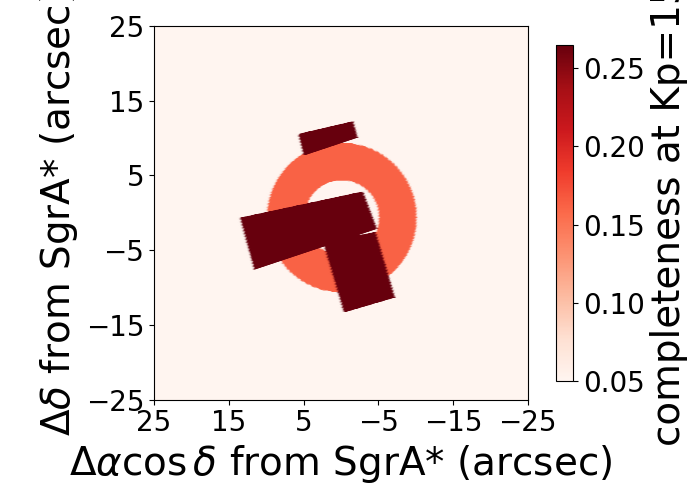
When determining which completeness to use for each star, we first need to determine whether this star is within our GCOWS field. If a star is within our GCOWS field, we will use the higher completeness fraction between GCOWS and Feldmeier-Krause et al. 2015. Otherwise, completeness from Feldmeier-Krause et al. 2015 will be applied. An example of our completeness map at = 15 is shown in Figure 3.
II.4 Position, Proper motion and Acceleration
Projected positions and proper motions on the sky are derived from high-resolution, infrared (IR) images obtained over a 1025 yr time-baseline. Depending on the distance from Sgr A*, we either use observations from the 10 m telescopes at the W. M. Keck Observatory (WMKO) or the Hubble Space Telescope (HST), as described below.
(1) The central 10″ 10″ region of the GC (approximately centered on Sgr A*) has been monitored with diffraction-limited, near-infrared imaging cameras at WMKO since 1995. For stars in this region, we have the longest time baseline and the highest spatial resolution, which gives precise proper motions and even significant accelerations on the sky plane. The complete catalog of measured positions, proper motions, and accelerations and analysis details is presented in Jia et al. 2019.
(2) To measure the proper motions of the young stars at larger radii, we use a widely dithered mosaic of shallow Keck IR images covering a 22″ 22″ FOV as described in Sakai et al. 2019. The astrometric uncertainties in this mosaicked dataset are typically larger than in the central 10″ data, because of the shorter time baseline and lower SNR.
(3) For stars at even larger radii (R 75), we use proper motions measured from the HST WFC3-IR instrument. This dataset consists of 10 epochs of observations centered on Sgr A* that were obtained between 2010 – 2020 in the F153M filter (2010.5: GO 11671/PI Ghez, 2011.6: GO 11671/PI Ghez, 2012.6: GO 12318/PI Ghez, 2014.1: GO 13049/PI Do, 2018.1: GO 15199, PI Do, 2019.2: GO 15498/PI Do, 2019.6: GO 16004/PI Do, 2019.7: GO 16004/PI Do 2019.8: GO 16004/PI Do, 2020.2: GO 15894/PI Do). While the HST spatial resolution is 2.5 times lower than that achieved with the Keck observations (FWHM 0.17" versus FWHM 0.06"), HST’s FOV of 120" 120" is much larger than can be realistically achieved with current AO systems. The astrometry from each HST epoch is first transformed into the Gaia absolute reference frame (Mignard & Klioner 2018) and then further transformed into the AO reference frame via 2nd-order bivariate polynomial transformations. The resulting HST catalog achieves an average precision of 0.33 mas and 0.07 mas/yr for the positions and proper motions of the stars in the sample. A detailed description of the HST catalog will be provided in a future paper (Hosek et al., in prep).
II.5 Photometry and Extinction
To ensure that our final sample shares a common photometric system, we adopt the Kp magnitude for each star from the deep wide mosaic image analysis reported in Lu et al. 2013 which covers all 88 stars in our sample. The Kp magnitude for each star is reported in the Kp column in Table 8. Then we applied the latest extinction map from Nogueras-Lara et al. 2018 to differentially de-redden all stars to a common , and the extinction corrected magnitude is reported as in Table 8.
III ORBIT ANALYSIS
For stars with measured (, , , , , ), the six Keplerian orbit parameters (inclination , angle to the ascending node , time of periapse passage , longitude of periapse , period , and eccentricity ) can be analytically determined if the central potential is known (Lu et al. 2009). §III.1 describes the Monte Carlo process used to estimate stars’ orbital parameters given prior estimates on the central potential. For stars that show significant acceleration (S0-1, S0-2, S0-3, S0-4, S0-5, S0-8, S0-16, S0-19, S0-20), their orbits are best constrained by simultaneously fitting the astrometry and RV measurements as a function of time (Do et al. 2019). §III.2 describes the computationally expensive orbit fitting procedure used for these 9 stars.
III.1 MC analysis for stars with (, , , , , )

Orbital parameters are determined for the 79 stars without significant acceleration measurements using a Monte Carlo (MC) analysis as described in detail in Lu et al. 2009 and Yelda et al. 2014. Each star has measurements of the line-of-sight velocity () as described in §II.2 and proper motion parameters (, , , ) as described in §II.4. The absolute value of the line-of-site distance || between the star and Sgr A∗ can be calculated from the following equation if is known.
| (3) |
Here, is the 3D distance and is the 2D projected sky-plane distance from Sgr A*, where . We note that there is a sign ambiguity in the line-of-sight distance.
We sample the 6 measured position, velocity, and acceleration quantities times assuming a Gaussian distribution for each measurement and its uncertainty. For each sample, the 6 Keplerian orbital parameters are analytically determined assuming an enclosed mass and distance to the Galactic Center as described below. The MC simulations produce a joint probability density function (PDFs) for the 6 orbital parameters.
The mass distribution giving rise to the central potential, , is a combination of the SMBH mass and an extended mass profile:
| (4) |
The adopted SMBH properties include a mass of = (3.975 0.058) and a distance of = (7.959 0.059) kpc, based on the analysis of S0-2’s orbit (Do et al. 2019). We used the extended mass profiles from Trippe et al. 2008 and found that adding extended mass has limited impact on the orbit analysis. We nonetheless adopt an extended mass profile with
| (5) |
where and the break radius is = 8.9″. We have also tried other extended mass profiles, like that of Schödel et al. 2009, and the results are similar.

Among the 79 stars, 45 have precise and accurate astrometry from Jia et al. 2019 with well-measured proper motions and constraints on the projected acceleration, , as shown in Table 8. However, not all measured values are physically allowed for a single star on a bound orbit around the supermassive black hole and enclosed extended mass. The maximum allowed is set by the gravitational acceleration when = 0 pc and we constrain the minimum allowed to be the acceleration at a distance of = 0.8 pc:
| (6) |
The maximum is chosen to be 0.8 pc because very few young stars are detected outside 0.4 pc and the most distant young star detected in our sample is at 0.6 pc. If the distribution of young stars is approximately spherically symmetric about the black hole, then the maximum line-of-sight distance should not exceed 0.8 pc. If a stars’ measured ( 2) overlaps with the allowed range, we draw its in each MC trial from a Gaussian distribution with the mean set to the measured , the standard deviation set to the measured , and truncated to the allowed range. This is the case for 35 stars. For the rest of the stars without a significant or physical , we use a uniform distribution in the range of allowed . In Figure 4, we use three stars as an example to show how is simulated in the MC analysis. The last column in that plot shows the distribution of and its limits ( and ) in red dashed lines, while the orange histogram is the probability density function for simulated .
The uniform acceleration prior, in the absence of other constraints, may lead to biased results in angular momentum measurements as shown in Yelda et al. 2014. It produces a deficit of stars close to z=0 as shown in Figure 4 and von Fellenberg et al. 2022, Fig. 12. However, as discussed above, we only apply this prior for roughly half of the stars that do not have a physically allowed or significant , most of which are located at larger radii where the bias is less apparent. Thus the choice of a uniform acceleration prior does not strongly bias the results.
Even for those 35 stars with measured within the allowed range, the significance of their accelerations varies. This is due to many factors, including the location of the star, the brightness of the star, the number of epochs in which the star is detected, etc. A more precise acceleration will result in more precise orbital parameters. In Figure 4, both S1-3 and S3-190 have a measurement-based prior, while S7-10’s prior is uniform over the allowed range. S1-3 has a 40 significant acceleration, but S3-190 only has 1 significant acceleration. As a result, S1-3 has much more constrained orbital parameters compared to S3-190. For S7-10 with a uniform prior, its orbital parameters are even less constrained. The distribution for S7-10 decreases with increasing radius even when is evenly distributed, which agrees with observation and validates the uniform prior.
III.2 Full Keplerain orbit fit for central stars
For stars with time-variable RV, we inferred their orbital parameters by simultaneously fitting spectroscopic and astrometric measurements. We utilized the same orbit-fitting procedure as was used by Do et al. 2019 to test General Relativity using the orbit of S0-2. From the orbit-fit posterior distributions, we drew 105 samples in order to match the posterior sample size for stars with a single RV from §III.1. S0-1, S0-2, S0-3, S0-4, S0-5, S0-8, S0-16, S0-19, S0-20 in our sample are fitted this way. We adopted the observable-based prior paradigm from O’Neil et al. 2019 that is based on uniformity in observables to improve orbital solutions for low-phase-coverage orbits. A full Keplerian orbit fit for S0-2 is shown in Fig 5. All 9 stars’ fitted results are attached in appendix C.
IV Disk Membership Analysis
IV.1 Detecting Stellar Disks
Each star’s orbital plane can be uniquely described by a unit normal vector L that is perpendicular to the orbital plane. This normal vector L can be expressed in terms of the inclination () and the angle to the ascending node () (see Equation 8 in Lu et al. 2009). Stars moving in a common plane share a common normal vector. In order to detect a stellar disk or stream, we adopt a nearest-neighbor method similar to that used by Lu et al. 2009 and Yelda et al. 2014. In this method, the sky is divided into 49152 pixels with equal solid angle area and for a given MC simulation the density at each (, ) position is calculated using the following equation:
| (7) |
where is the angle to the th nearest star and we use = 6. The resulting average density is nearly the same for other choices of = 4, 5, or 7. Then the combined density map is an average over all 105 MC trials from §III. The resulting density maps are presented in §V.

IV.2 Disk/Plane Membership Probabilities
With the disk or plane normal-vectors and uncertainties determined from §IV.1, the membership probability, , can be estimated for each star following Lu et al. 2009.
| (8) |
| (9) |
Here SA is the solid angle measured at the contour where the disk density drops to half of the peak value; is the integration of each star’s density map over the stellar disk region, and is the integration over its own peak region with the same SA.
In summary, each star’s is integrated inside the disk or plane area and normalized by the star’s peak probability over a similar area. Thus, stars with large uncertainties in and will only have high plane membership if they are centered on the plane. The final disk or plane memberships are presented in §V.
V Results
V.1 Two Stellar Disks

The density map of normal vectors, L, shows two over-dense regions, indicating the presence of at least two distinct populations, each of which consists of stars that share a common orbital plane (Figure 6). We label the two peaks as Disk1 and Plane2. The well-known clockwise (CW) disk is the upper right Disk1 located at (, ) = (124°, 94°), consistent with the past measurements of the disk location (Levin & Beloborodov 2003; Genzel et al. 2003; Paumard et al. 2006; Lu et al. 2009; Bartko et al. 2009; Yelda et al. 2014; von Fellenberg et al. 2022). We found another almost edge-on plane which we call Plane2, located at (, ) = (90°, 245°). This may be the same structure identified as F3 in von Fellenberg et al. 2022; Plane2 and F3 have similar eccentricity and semi-major axis distributions, along with of common members. However, the two features are 30 apart in terms of : von Fellenberg et al. 2022 found F3 has (, ) = (102°, 211°) after conversion to our reference frame. A more detailed comparison is presented in Appendix B. The uncertainty in the location of each of the planar features is defined to be where the density drops to 50% of its peak value and it is marked with a black dashed line in Figure 6. The uncertainties for Disk1 and Plane2 are (, ) = (15°, 17°), (, ) = (20°, 19°). We also estimate the fraction of young stars belonging to each structure by calculating the sum of the membership probabilities over the total 88 young stars and found that of our sample belongs to Disk1 while belongs to Plane2.
To quantify the significance of both disks, we simulated an isotropic population with synthetic (, , , , ) and extracted orbits in the same way as on the real data. Each simulated star was first assigned a 2D radius on the sky, , and a 3D velocity, , drawn from the observed young stars. Then the orientation of the position and velocity vectors were randomly generated (Yelda et al. 2014). Any measurements of were kept fixed in amplitude and uncertainty. For the 9 stars from §III.2 with well-measured orbits, we drew 105 samples from randomized and with their posterior distribution uncertainty. The significance of Disk1 and Plane2 is defined by:
| (10) |
where is the density of the stellar disk at its peak, is the density of the isotropic simulation at the same position, and is the dispersion of the density at the peak among all the isotropic simulations at the same position. A summary of the peak density, significance, and the simulated isotropic density and its dispersion is presented in Table 2.
The significance for Disk1 is 12.4 and Plane2 has a significance of 6.4. The reason we have a slightly lower significance for Disk1 compared to Yelda et al. 2014 is because we have a smaller sample size due to our requirement that only stars from surveys with published completeness curves can be included. As a result, our uncertainty in the isotropic density is slightly larger.
The significance of Plane2 is only slightly higher than previously claimed planar structures and disks that were later shown to be statistically insignificant (Paumard et al. 2006; Bartko et al. 2009; Lu et al. 2009). Thus, we must be cautious in claiming a new dynamical structure. Unlike previous claimed structures, the Plane2 structure is the result of both numerous stars with moderate membership probabilities and at least 5 stars with .
| Structure | Solid Angle | Significance | Disk Fraction aaThis is calculated as sum of membership probabilities of stars belonging to each structure divided by the total 88 young stars. | ||||
|---|---|---|---|---|---|---|---|
| (°) | (°) | (sr) | (stars/deg2) | (stars/deg2) | |||
| Disk1 | 124 15 | 94 17 | 0.20 | 0.013 0.006 | 0.003 0.0008 | 12.4 | 0.084 |
| Plane2 | 90 20 | 245 19 | 0.37 | 0.007 0.002 | 0.002 0.0007 | 6.4 | 0.060 |
The probability of each star belonging to Disk1 or Plane2 is given in Table 3. To view stars in Disk1 and Plane2 in a more direct way, we make a quiver plot showing the proper motion of each star in Figure 7. For illustrative purposes, we identify high-probability disk members as those with ; and Disk1 and Plane2 stars are shown as red and blue arrows, respectively. We note that all disk membership probabilities are calculated assuming the existence of only that disk. We choose not to determine disk membership using a more complex mixture model based on two simulated disks plus an isotropic population as it would require a prior knowledge of the disk properties such as the eccentricity and semi-major axis distributions.
| Name | PDisk1 | PPlane2 | SA |
|---|---|---|---|
| S0-1 | 0.00 | 0.00 | 0.001 |
| S0-11 | 0.00 | 0.05 | 0.081 |
| S0-14 | 0.00 | 0.00 | 0.004 |
| S0-15 | 0.76 | 0.00 | 0.004 |
| S0-16 | 0.00 | 0.42 | 0.001 |
| S0-19 | 0.00 | 0.00 | 0.002 |
| S0-2 | 0.00 | 0.00 | 0.000 |
| S0-20 | 0.00 | 0.00 | 0.001 |
| S0-3 | 0.00 | 0.00 | 0.000 |
| S0-30 | 0.00 | 0.00 | 0.106 |
| S0-31 | 0.00 | 0.30 | 0.004 |
| S0-4 | 0.00 | 0.00 | 0.001 |
| S0-5 | 0.00 | 0.00 | 0.001 |
| S0-7 | 0.00 | 0.00 | 0.001 |
| S0-8 | 0.00 | 0.00 | 0.001 |
| S0-9 | 0.00 | 0.00 | 0.003 |
| S1-19 | 0.43 | 0.00 | 0.022 |
| S1-2 | 0.50 | 0.00 | 0.004 |
| S1-22 | 0.54 | 0.00 | 0.189 |
| S1-24 | 0.00 | 0.00 | 0.003 |
| S1-3 | 0.49 | 0.00 | 0.007 |
| S1-33 | 0.00 | 0.00 | 0.122 |
| S1-4 | 0.02 | 0.00 | 0.081 |
| S1-8 | 0.00 | 0.00 | 0.003 |
| S10-185 | 0.00 | 0.73 | 0.132 |
| S10-232 | 0.00 | 0.00 | 0.578 |
| S10-238 | 0.00 | 0.78 | 0.002 |
| S10-32 | 0.18 | 0.00 | 0.119 |
| S10-34 | 0.00 | 0.00 | 0.517 |
| S10-4 | 0.00 | 0.00 | 0.087 |
| S10-48 | 0.00 | 0.00 | 0.037 |
| S10-50 | 0.00 | 0.00 | 0.400 |
| S11-147 | 0.00 | 0.00 | 1.322 |
| S11-176 | 0.00 | 0.00 | 0.237 |
| S11-21 | 0.04 | 0.00 | 0.174 |
| S11-214 | 0.00 | 0.00 | 0.131 |
| S11-246 | 0.00 | 0.01 | 0.209 |
| S11-8 | 0.00 | 0.00 | 0.784 |
| S12-178 | 0.00 | 0.03 | 0.008 |
| S12-5 | 0.00 | 1.00 | 0.003 |
| S12-76 | 0.00 | 0.00 | 0.257 |
| S14-196 | 0.00 | 0.00 | 0.410 |
| S2-17 | 0.37 | 0.00 | 0.009 |
| S2-19 | 0.24 | 0.00 | 0.071 |
| S2-21 | 0.50 | 0.00 | 0.018 |
| S2-4 | 0.22 | 0.00 | 0.007 |
| S2-50 | 0.00 | 0.00 | 0.188 |
| S2-58 | 0.00 | 0.00 | 0.188 |
| S2-6 | 0.50 | 0.00 | 0.009 |
| S2-74 | 0.50 | 0.00 | 0.044 |
| S3-19 | 0.36 | 0.00 | 0.357 |
| S3-190 | 0.35 | 0.00 | 0.084 |
| S3-26 | 0.24 | 0.24 | 0.163 |
| S3-3 | 0.00 | 0.00 | 0.467 |
| S3-30 | 0.00 | 0.00 | 0.012 |
| S3-331 | 0.00 | 0.00 | 0.103 |
| S3-374 | 0.00 | 0.00 | 0.086 |
| S3-96 | 0.00 | 0.00 | 0.351 |
| S4-169 | 0.40 | 0.00 | 0.420 |
| S4-262 | 0.00 | 0.00 | 0.117 |
| S4-314 | 0.47 | 0.00 | 0.231 |
| S4-364 | 0.00 | 0.00 | 0.296 |
| S4-71 | 0.00 | 0.00 | 0.012 |
| S5-106 | 0.00 | 0.34 | 0.029 |
| S5-183 | 0.00 | 0.00 | 0.094 |
| S5-191 | 0.00 | 0.00 | 0.612 |
| S5-237 | 0.00 | 0.00 | 0.247 |
| S6-63 | 0.27 | 0.00 | 0.215 |
| S6-81 | 0.00 | 0.00 | 0.086 |
| S6-89 | 0.00 | 0.00 | 0.398 |
| S6-96 | 0.00 | 0.00 | 0.411 |
| S7-10 | 0.16 | 0.03 | 0.285 |
| S7-216 | 0.00 | 0.00 | 0.153 |
| S7-236 | 0.00 | 0.00 | 0.873 |
| S7-30 | 0.00 | 0.00 | 0.592 |
| S7-5 | 0.05 | 0.00 | 0.499 |
| S8-10 | 0.00 | 0.00 | 0.769 |
| S8-126 | 0.00 | 0.00 | 1.139 |
| S8-196 | 0.00 | 0.22 | 0.142 |
| S8-4 | 0.00 | 0.00 | 0.032 |
| S8-5 | 0.00 | 0.00 | 0.370 |
| S8-8 | 0.01 | 0.00 | 0.271 |
| S9-143 | 0.01 | 0.00 | 1.220 |
| S9-221 | 0.00 | 0.77 | 0.044 |
| S9-6 | 0.04 | 0.00 | 0.267 |
| IRS 13E1 | 0.00 | 0.50 | 0.002 |
| IRS 16CC | 0.25 | 0.00 | 0.070 |
| IRS 33N | 0.00 | 0.00 | 0.004 |
V.2 Disk Properties
In this section, we compare the distribution of eccentricities (), radial distances on the disk plane (derived in §V.2.2) and disk thickness for the different dynamical subgroups. We then use this distribution as the input prior for disk simulations in §V.3.
V.2.1 Eccentricity Distribution
Stars are divided into Disk1, Plane2 and Non-disk stars using membership probabilities as weights rather than through a hard probability cut. We assign a weight to each MC trial among the trials for every star (§III). For a particular MC trial with a set of Keplerian orbital parameters (, , , ), the weight of being on Disk1 (WDisk1), Plane2 (WPlane2) and Non-disk (WNon-disk) structures are calculated as:
| (11) |
where N(, ) is normal distribution with mean of and standard deviation of .


We modeled the underlying eccentricity distribution for Disk1, Plane2, and the Non-disk populations separately. We used a hierarchical Bayesian inference (HBI) method similar to Hogg et al. 2010 and Bowler et al. 2020 to infer the population-level eccentricity distribution of each sub-structure. This method was proposed first in constraining the population-level eccentricity distribution of exoplanets, where a standard maximum-likelihood estimator of eccentricity is biased to a high value. HBI is especially useful when, as shown in Bowler et al. 2020, the measured eccentricity posteriors for individual stars vary significantly with some well constrained, others poorly determined, and most with asymmetric or non-Gaussian probability distributions (Wolfgang et al. 2016; Eylen et al. 2019, see also).
To apply this framework to our case, we first adopted a Beta distribution for the eccentricity distribution for each population,
| (12) |
where is the usual Gamma function defined as . Recall that a Beta function can reproduce distributions that are uniform (), peaked at low (small ), peaked at high (small ), and anything in between, which makes the distribution very flexible. We then used HBI to find the most probable and parameters for each population’s eccentricity distribution, solving for
| (13) |
where describes the population’s eccentricity distribution, is the set of orbital parameters for each star, , and is the data for each star. This enables us to use posterior samples from an individual star’s eccentricity distribution to estimate the population’s distribution. As we already have posterior samples for the individual stars’ orbital parameters, , similar to Bowler et al. 2020, we can write the posterior distribution of hyper-parameters as:
| (14) |
where is the prior on the hyper-parameters. Then we can approximate the likelihood for the population parameters by importance sampling the existing posteriors with
| (15) |
where is the eccentricity of the -th draw for star as described in Hogg et al. 2010 and is the membership probability for each star. The orbital parameter posteriors for most stars were generated using a Monte-Carlo sampling method and an explicit eccentricity prior was not utilized. However, the uniform prior produces a fairly uniform eccentricity distribution; thus we assume that is uniform. Priors on and were uniform from [0, 50] and [0, 30], respectively. The final posterior probability distribution on was inferred using the nested sampling package, Dynesty (Speagle 2020; Skilling 2004; Skilling 2006; Feroz et al. 2009; Higson et al. 2019).
The best-fit eccentricity distributions are plotted in Figure 8. For the Disk1 population, we see a peak at = 0.36, which is consistent with the previous determination by Yelda et al. 2014, but with a larger spread, implying more high eccentric orbits in Disk1. For the Plane2 population, the eccentricity distribution is shifted to higher eccentricities, although the uncertainties are large, given the small number of stars. We adopt the maximum-likelihood solution for all three populations, including Plane2, even though the intrinsic eccentricity distribution is uncertain and may have a different functional form. For the Non-disk stars, the distribution is fairly flat, with a slight preference for higher eccentricities. Both the Plane2 and Non-disk populations are consistent, within uncertainties, with a relaxed population, which should scale as ; however, a non-relaxed, but high, eccentricity distribution is preferred (Figure 9). To summarize, we find that the eccentricity distributions are described by:
| (16) |
V.2.2 Radial Profile
In order to calculate a star’s radial position on the disk, we first need to find its projected position vector on the disk plane. We have the and positions for each star and thus we need to calculate on the disk plane. To do this, we begin by finding the normal vector to the disk, L, from its and :
| (17) |
After calculating the normal vector , combined with known and positions of stars, we find by projecting stars onto the disk plane:
| (18) |
then the radial distances are calculated by Pythagorean Theorem.
To create the PDFs of the distributions for both Disk1 and Plane2, we sample both stars and structures simultaneously. First, a sample of and is drawn for each star from its MC result times. Second, another sample of each structure’s and is created by drawing times from a Gaussian distribution defined by the means and uncertainties of and shown in Table 2. We randomly match elements of these two samples to create a new data set, where each data set contains one combination of a star’s and and a disk’s and . From this new data set, we calculate values for each combination using Eqs. 17 and 18. Additionally, we imposed a cut of 20 parsecs on our values of because these dynamical sub-structures, especially Plane2, are close to edge-on.. Without this cut, we would obtain values of approaching infinity.
We also calculate a weight associated with each data in the following way, assuming no change in uncertainty of disk parameters and a normal distribution.
| (19) |
This is the probability of each sampled star being located on the sampled disk. We do not use membership probability because it is an integrated result and could not reflect details of sampled data. Then a weighted histogram of 88 stars is created for each sampled disk’s and . Each histogram is normalized by 2D bin widths (i.e. annular area between each bin) to account for the 2D geometry of disk structure. The final PDF of for each structure is obtained by taking the mean across these histograms and the uncertainties are estimated by the standard deviation. For the off-disk population, there is no disk to project the stars onto, so the stars’ radial positions on the plane of the sky are considered. An distribution is then created through a normalized distribution of the data. The uncertainties of these data points are estimated by the Poisson error on each data point.
The data were fit using Bayesian inference with multi-nested sampling by the Dynesty python package. From inspection, we decided to fit the distribution by a truncated single power-law for all three structures. Thus we only need to fit for the slope parameter .
To estimate the uncertainty of the model, we sampled the posterior distributions of the model parameters 200 times, each time recalculating the model. We estimate the uncertainty by taking the standard deviation of all these calculated models. The radial distributions and best-fit models for the three subgroups are shown in Figure 10.
We find that that the radial position distribution in the disk and the sky are described by:
| (20) |
We initially fit the distribution of Disk1 by the truncated broken power law with model parameters , , and . However, this results in huge uncertainties on model parameters. To justify our choice of a single power law, we compare values of both the Bayesian Information Criterion (BIC) and Akaike Information Criterion with small sample modification (AICc) for these two models. The results are shown in Table 4. From this table, the difference between BIC values of Disk1 for different models is 2, which suggests moderate evidence against single power law. However, the AICc strongly prefers a single power law with difference of about 10. Thus we conclude that there is no preference between these two models for Disk1 and we choose to present the single power-law result because it has well constrained parameters. Similar reasoning applies to the off-disk population. For the Plane2 population, we prefer a single power law due to its few data points compared to the number of parameters.
| Model | Structure | BIC | AICc |
|---|---|---|---|
| Single Power Law | Disk 1 | 20.72 | 21.93 |
| Broken Power Law | Disk 1 | 19.85 | 32.48 |
| Single Power Law | Plane 2 | 5.45 | 8.07 |
| Broken Power Law | Plane 2 | 8.08 | N/A aaAICc does not apply to Plane2 because the number of data points equals to the number of parameters plus one, which rejects Broken Power Law model (overfitting). |
| Single Power Law | Non-disk | 15.78 | 15.98 |
| Broken Power Law | Non-disk | 12.99 | 16.08 |
The thickness of the disk can be estimated using the velocity dispersion perpendicular to the disk plane. Here we follow the process described by Lu et al. 2009. First, each potential disk candidate’s three-dimensional velocity, , is projected into the direction of . The uncertainty of both and are taken into consideration when calculating intrinsic velocity dispersion , where = . Then the disk’s scale height () can be derived from the ratio of and <> , where is the intrinsic velocity dispersion, and <> is the average magnitude of the 3D velocity of disk candidates, weighted their by disk membership probability. Finally, this scale height can be related to disk thickness described in terms of disk-opening angle . For Disk1, we find = 33 km s-1, giving a scale height of 0.09 0.01 and a disk-opening angle of 7.0° 0.9°, consistent with previous results (Lu et al. 2009; Yelda et al. 2014). For Plane2, we find = 58 km s-1, giving a scale height of 0.23 0.07 and a disk-opening angle of 18.6° 6.2°.
V.3 Simulations
| Parameters | Disk1 | Plane2 | Non-disk |
|---|---|---|---|
| N (, ) | N (, ) | P() cos() | |
| N (, ) | N (, ) | Uniform(0°,360°) | |
| Uniform(0°,360°) | Uniform(0°,360°) | Uniform(0°,360°) | |
| bbFor simulated cluster, we choose to only use peak parameters corresponding to max likelihood. | |||
| ccEqu 20. Here we use to represent the radial distance . For each broken power law, we choose pc and pc. | bbFor simulated cluster, we choose to only use peak parameters corresponding to max likelihood. | ||
| Uniform(1995, 1995+period) | Uniform(1995, 1995+period) | Uniform(1995, 1995+period) | |
| 1 | 1 | 1 | |
| 150 | 150 | 150 | |
| 105 | 105 | 105 | |
| Age | 6Myr | 6Myr | 6Myr |
| IMF | |||
| distance | 8kpc | 8kpc | 8kpc |
From Figure 7, we can see the spatial distribution within each disk plane does not appear symmetric, especially for Plane2 stars. Intrinsic asymmetry is important in understanding and constraining the subgroup’s dynamical history. However, there are many reasons that can lead to this observed asymmetry: extinction, incomplete observation, and intrinsic asymmetry. In order to characterize this asymmetry, we simulate the whole cluster and each dynamical sub-structure using properties determined in §V.2. We also take inverse-completeness (see §II.3) and the full extinction map from (Schödel et al. 2010) into account when doing the simulation in order to diminish the effects from these two factors. Then we compare the simulated stellar distribution to the observed one to explore whether the structure is intrinsically asymmetric or not.
Table 5 summarizes the input simulation parameters. First, we use an open-source python package SPISEA (Hosek et al. 2020) to generate a single age (6 Myr) star cluster with solar metallicity, located 8 kpc away. The total mass of the simulated cluster is 10, with minimum mass of 1 M⊙, maximum mass of 100 M⊙, and a power-law IMF with a slope of -2.35 (Salpeter 1955). While the IMF for the YNC has been shown to be top-heavy (Bartko et al. 2009; Lu et al. 2013), the analysis of the kinematic and spatial sub-structure is relatively insensitive to the choice of IMF and total cluster mass as we re-scale the simulated clusters to match observed stellar densities. We generate the synthetic photometry for each star in the NIRC2 Kp filter, assuming a fixed extinction value of AKs = 2.7 mag, for easy comparison to the observed Kpext shown in Table 8. In this step, we assume the three dynamical subgroups have the same age, IMF, and extinction.
The cluster generated by SPISEA gives mass and Kpext for every star in the system. However, our analysis excludes all WR stars because the generated values of mass and Kpext are less trustworthy compared to non-WR stars. The next step is to assign a position for each star based on their dynamical subgroup. We use the disk properties from §V.2 to simulate positions for Disk1, Plane2 and Non-disk stars. To account for differential extinction over the field of view, which introduces asymmetric features in the observed distributions, we redden the Kpext back to observed Kp using the full extinction map from Schödel et al. 2010 and then apply an inverse completeness map from §II.3 to account for stars that would not be observable. This approximates how the simulated cluster would appear in observations. The comparison of the observed stellar density profile with the simulated density profile is shown in Figure 11. We present the density profile in polar coordinates, where North is at 90°and West is at 0°, so that it is easier to see the azimuthal structure in each dynamical subgroup. These plots have the same orientation as they appear on the sky.
For the Non-disk group, the sub-structure is mainly caused by the differential extinction, and our simulation reproduces the observation well within uncertainties. This indicates that the Non-disk group is nearly isotropic. For Disk1 and Plane2, we expect an over-density in their disk plane, which can be seen in both the observed and simulated maps. However, for Plane2, the observed density on the Southwest side is significantly more dense than the observed density on the Northeast side (left plot of (c) in Figure 11), which is less significant in the simulated stellar distribution (right plot of (c) in Figure 11). Because we have taken both completeness and extinction into account when doing the simulation, this difference between observed and simulated stellar distribution should be explained by reasons other than these two factors. Thus, we think this difference implies that Plane2 is intrinsically asymmetric and may be a stream rather than a plane.


VI Discussion
The presence of multiple sub-structures in the young nuclear cluster implies that star formation occurred in dynamically complex gas structures around the SMBH. We can infer that the structures that are observed today are related, but not identical, to the initial gas structure since the two-body relaxation timescale is longer ( 30 Myr 1 Gyr Kocsis & Tremaine 2011) than the age of the YNC (3 8 Myr Lu et al. 2013). However, some dynamical evolution is expected due to vector resonant relaxation at radii (0.04 pc) and resonant friction at larger radii. In particular, Levin 2022 notes that resonant friction can take a single disk and smear it into transient streams with different orientations in only a few Myrs. Note, the asymmetric gravitational potential due to the surrounding circum-nuclear disk at a few pc may dampen these resonant dynamical processes. More precise theoretical simulations are needed to run back the clock from the sub-structures observed today to the initial configuration at the time of star formation. More detailed discussion is presented below.
VI.1 Comparisons to Previous Work
While the CW disk has been verified many times in previous work (Levin & Beloborodov 2003; Genzel et al. 2003; Paumard et al. 2006; Lu et al. 2009; Yelda et al. 2014; von Fellenberg et al. 2022), other kinematic structures in the young nuclear cluster have been controversial. A counter-clockwise (CCW) disk was originally reported in Genzel et al. 2003 and confirmed in Paumard et al. 2006. Later work (Bartko et al. 2009; von Fellenberg et al. 2022) found that the CCW disk was highly extended, anisotropic, and showed evidence for a warped disk on large scales. However, this CCW disk was not detected by Lu et al. 2009 and Yelda et al. 2014 in an independent analysis with different observations for RVs and proper motions. In the work presented here, we confirm the existence of the CW disk, with properties consistent with previous analyses, and we also do not detect the CCW disk. Instead, we detect a second edge-on disk called Plane2 (c.f., §VI.4), which might be the same as the F3 structure reported in von Fellenberg et al. 2022 (c.f., §V.1, Appendix B.2).
A comparison of the locations of the CW disk, CCW disk and Plane2 on the density map is presented in Figure 12, from which we conclude that the position of Plane2 is clearly very different from that of the previously claimed CCW disk.

There are small discrepancies between our work and that of vF22 for the significance and locations of Disk1 and Plane2. These are likely due to significant differences in proper motions at small radii and large, but not statistically significant, differences in radial velocities. In addition, our requirement of spectroscopic completeness information for stars to be included in our sample yields an overall smaller number of young stars. Lastly, our use of a uniform acceleration prior (c.f., §III.1) on % of the stars at large radii may also influence structure detection.
The stars within 0.8″are more randomized by dynamical effects like vector resonant relaxation (Rauch & Tremaine 1996; Hopman & Alexander 2006; Alexander 2007), so the inner edge of the CW disk is roughly at 0.8″as reported in (Schödel et al. 2003; Ghez et al. 2005; Gillessen et al. 2009). This agrees with our analysis. In our sample, we have 14 young stars within 0.8″and all of them have zero probability of being on Disk1.
VI.2 CW Disk1 Properties
The stars in Disk1 are found to have non-circular orbits. Bartko et al. 2009 combined their results with those of Gillessen et al. 2009 and reported an eccentricity distribution with <> = 0.36 0.06. Yelda et al. 2014 divided stars into accelerating sources and non-accelerating 22 2 These stars also have accelerations but are insignificant that we cannot detect. sources, having <> = 0.27 0.09 and <> = 0.43 0.24, respectively. Our eccentricity distribution for Disk1 is shown in Figure 8 and has a peak at and <> = 0.39 0.16. Our result has a much larger uncertainty due to our requirement of only using data with completeness information, which results in a smaller overall sample. We performed an analysis similar to that of Yelda et al. 2014, dividing stars into accelerating and non-accelerating moving stars. The accelerating sources are defined in Jia et al. 2019, including 4 stars in our sample: S1-2, S1-3, S2-6 and S4-169. The comparison of distribution between accelerating and non-accelerating sources in Disk1 are plotted in Figure 13, which agrees with the conclusion from Yelda et al. 2014 - accelerating sources have a well constrained peaking at 0.2, while the distribution of non-accelerating sources has a much larger dispersion. Specifically, accelerating sources have <> = 0.25 0.12 while non-accelerating sources have <> = 0.45 0.24. The difference is likely due to accelerating sources having better constraints on their orbital parameters (see Figure 4).

Disk1 has a significant intrinsic thickness as was shown by Paumard et al. 2006; Lu et al. 2009 and Yelda et al. 2014. For example, Paumard et al. 2006 reported a disk opening angle of = 14° 4° and Lu et al. 2009 reported a disk thickness of = 7° 2°. Our intrinsic disk thickness of = 7° 1° is consistent with that found in previous work, only with smaller uncertainty.
The surface density profile in the plane of Disk1 is predicted to be (r) r-2 for in-situ formation scenarios (Lin & Pringle 1987; Levin 2007) and has been verified in many observations (Paumard et al. 2006; Bartko et al. 2009; Lu et al. 2009; Yelda et al. 2014). In our paper, the semi-major axis distribution was initially fit with methods similar to the eccentricity distribution as discussed in §V.2.1. However, the fit results were extremely uncertainty and no significant constraint could be placed on the distribution in the disk plane. We instead explore the distributions of projected radial distances on the disk plane. The slope of the radial profile ( from Eq.20) is in agreement with the predicted .
VI.3 Plane2 Properties
In addition to the CW Disk1, we found a new CCW structure Plane2, which has 10 stars out of the total 88 young stars in our sample. We estimated that Plane2 has , which is similar to the F3 structure reported in von Fellenberg et al. 2022. A more detailed comparison between these two structures is discussed in Appendix B.2 and B.3. As presented in §V.2.1, stars in Plane2 have relatively high eccentricities, with . We also estimated the intrinsic disk thickness of Plane2 to be . The radial profile of Plane2 has a power law index of from Eq.20, which is inconsistent with the predicted -2. This might be caused by the complex dynamical evolution experienced by Plane2 stars such that they have high eccentricities with less steep radial profile. One of the most prominent feature of Plane2 is its spatial asymmetry. As discussed in §V.3, this asymmetric feature cannot be explained by differential extinction or incompleteness and is likely intrinsic to the structure.
VI.4 Is Plane2 Related to the IRS 13 Group or G sources?
IRS 13 is a group of nearly co-moving massive young stars, clustered together at 3.5″to the West of the SMBH (Maillard et al. 2004; Paumard et al. 2006; Martins et al. 2007). It has been proposed to lie within the previously claimed CCW disk (Maillard et al. 2004; Schödel et al. 2005), but later works did not detect the CCW disk (Lu et al. 2009; Yelda et al. 2014), nor do we detect it in this work. Interestingly, one of IRS 13 group stars, IRS 13E1, is a potential Plane2 star, with a 50% probability being on Plane2. The remaining IRS 13 sources E2, E3, and E4, are currently not in our sample as they were excluded either due to their Wolf-Rayet star nature or the lack of published completeness information. Here we relax our requirement for a complete sample in order to identify other candidate Plane2 members; although we note that we cannot infer structural properties of Plane2 from this analysis.
Since all the IRS 13 stars are moving in approximately the similar direction, we run the same orbital and disk membership analysis for three other IRS 13 stars in addition to IRS 13E1. They are IRS 13E2, IRS 13E3, IRS 13E4. We use the most up-to-date radial velocities reported in Zhu et al. 2020. Note that using RV measurements from Paumard et al. 2006 and Bartko et al. 2009 generates similar results. The proper motions for IRS 13 stars are plotted in Figure 14 and the (, ) density map is shown in Figure 15. Note that the nature of IRS 13E3 is not entirely clear – it may be a dusty star or a gas clump at the intersection of colliding winds (Zhu et al. 2020; Wang et al. 2019; Fritz et al. 2010) and the proper motion is quite uncertain (Tsuboi et al. 2022; Fritz et al. 2010). Nevertheless, we find that IRS 13E3 is a potential Plane2 star, with a disk membership probability PPlane2 = 0.34, but IRS 13E2 and IRS 13E4 are not on Plane2 with PPlane2 < . Based on the posterior contours of IRS 13E2 and IRS13 E4 in the (, ) plane, we think they are close to F1/CCW feature reported in von Fellenberg et al. 2022; however, they did not classify these two IRS13 stars as belonging to F1/CCW feature.
Even though all four IRS 13 stars are approximately moving in a similar direction on the sky, the dispersion in the proper motions of the stars is significant. Recent studies of E1’s proper motion propose that this star may not be bound to the IRS13 group, while E2 and E4 are most likely bound to the group (Wang et al. 2019; Mužić et al. 2008). Additionally, studies of the spectrum of IRS 13E1 and E2 do not show signs of binarity (Fritz et al. 2010). The two different pairs (E1 & E3 and E2 & E4) are discrepant enough that they may not be associated with each other. Thus it is unclear whether Plane2 is related to the potentially bound IRS13 group given the low Plane2 membership probability for E2 & E4. Further study, including higher-resolution images and continued astrometric and RV monitoring will be needed to resolve the relationship between the apparently bound IRS 13 group and Plane2.
In order to include as many Plane2 stars as possible, we report all potential Plane2 stars based on our analysis of all 146 stars with reported RVs and proper motions, listed in Table 7. The potential Plane2 stars and their disk membership is reported in Table 6. A quiver plot showing the proper motion and RV for those potential Plane2 stars (PPlane2 > 0.2) is shown in Figure 16.
| Name | PPlane2 | SA |
|---|---|---|
| S0-31 | 0.30 | 0.004 |
| IRS 16NW | 0.38 | 0.046 |
| IRS 13E1 | 0.50 | 0.002 |
| IRS 13E3 | 0.34 | 0.265 |
| S4-258 | 0.40 | 0.093 |
| S5-34 | 0.36 | 0.034 |
| S5-106 | 0.34 | 0.029 |
| S5-236 | 0.71 | 0.024 |
| S9-114 | 0.52 | 0.063 |
| S9-221 | 0.77 | 0.044 |
| S10-185 | 0.73 | 0.132 |
| S10-238 | 0.78 | 0.002 |
| S12-5 | 1.00 | 0.003 |
| S13-3 | 0.27 | 0.133 |
| S0-16 | 0.42 | 0.001 |
| S3-26 | 0.24 | 0.163 |
| S8-196 | 0.22 | 0.142 |


A population of dust enshrouded objects are found to orbit around the SMBH: the so-called G sources. The most famous G source is G2, which first looked like a pure gas cloud (Gillessen et al. 2013; Eckart et al. 2013; Phifer et al. 2013), yet survived through closest approach to SgrA∗ in early 2014 (Gillessen et al. 2013; Abarca et al. 2014; Shcherbakov 2014; Witzel et al. 2014; Valencia-S. et al. 2015). This implies that G2 must contain a stellar-like object and is perhaps a binary merge product. However, there is still no broad consensus as to the origin and nature of the G sources. Using the near-infrared (NIR) spectro-imaging data obtained over 13 years at the W. M. Keck Observatory with the OSIRIS integral field spectrometer, Ciurlo et al. 2020 reported four more additional G sources, making the total number of G sources to six. Ciurlo et al. 2020 found the six G sources (G1, G2, G3, G4, G5 and G6) have widely varying orbits, suggesting G sources are formed separately. We compare the orbital plane direction for G sources with stellar disk plane and the individual G source (, ) density map is plotted in Figure 17. The conclusion is that none of the G sources are likely to be on either Disk1 or Plane2. However G5 is also edge-on, and has almost exactly 180°difference in compared to Plane2. In fact, there is a small probability of PPlane2 = 0.08 for G5 for its degenerate solution. In other words, G5 lies in the edge-on Plane2; but is counter-rotating in the plane.

VI.5 The Star Formation Process
Besides the widely accepted in-situ formation theory, it has been suggested that an inspiraling star cluster to explain the formation of young stars in our GC, where a massive young cluster migrate towards the center of the galaxy under dynamical friction (Gerhard 2001). However, this scenario will deposit stars with a profile of r-0.75, which is inconsistent with the observed density profile. So the fact that radial profile from §V.2 follows P(r) r-1.80 supports in-situ formation scenario.
Although we did not detect the counter-clockwise disk claimed in (Genzel et al. 2003; Paumard et al. 2006; Bartko et al. 2009), we found another almost edge-on disk (Plane2 in this paper) with highly asymmetric stellar distribution. This edge-on disk is mostly determined by stars on the southwest side and very few stars on the northeast side are found in this disk. While the uneven distribution of stars on Plane2 is not fully understood, possible explanations include: (1) The young stellar population is not uniformly distributed within Plane2, with more stars in the southwest region compared to northeast region (see §V.3). One possible situation that could explain this asymmetry is the non-uniform initial gas distribution, leading to uneven star formation. (2) If Plane2 is indeed related to the IRS13 group, the possible explanations for the formation of IRS13 group can also be used to explain Plane2. For example, Plane2 might be a remnant stream from the disruption of an IRS 13 cluster that may or may not contain an intermediate-mass black hole (IMBH) (Maillard et al. 2004).
VI.6 Biases Induced by Binaries
In our analysis of disk membership and disk properties, we assume that stars are not in binary systems. However, this may lead to biases in our results as presented by Naoz et al. 2018: if we ignore binaries, the disk memberships and disk fractions are likely to be biased to lower values; observed eccentricity and dispersion angle are likely to be biased to higher values.
Here we present an analysis of the influence of ignoring binaries on disk membership on each sub-structure, Disk1 and Plane2. We simulate a sample of stars drawn from each structure and generate 3D positions and velocities for each star based on the radial profile and eccentricity distribution presented in §V.2.1 and §V.2.2. Then we randomly assign each star as a binary or not based on the binary fraction of as is appropriate for massive stars (Raghavan et al. 2010; Stephan et al. 2016). If a star is assigned to be in a binary system, we assign its binary properties, such as binary eccentricity, mass ratio, and inclination, drawn from distributions of massive star binary properties described in Sana et al. 2012. The primary stellar masses are sampled based on the IMF described in Lu et al. 2013.
These binary properties, combined with position and velocity data of stars, are used to calculate a proxy parameter defined by Naoz et al. 2018, Eq 5. is the apparent deflection angle from the true orbital plane around the SMBH if the binary RV is ignored. We follow a similar criterion used in Naoz et al. 2018 §3, where a star with is considered as an on-disk star misidentified as an off-disk star. We simulate each structure 1000 times and calculate the mean fraction for , as shown in Figure 18.


We find that for Disk1, the misclassified disk fraction is and for Plane2 is . This implies that the presence of binaries should make of the on-disk stars appear as off-disk stars. Because we are ignoring binaries in our analysis, taking them into account would increase the Disk1 sample size from 18 stars to 21 stars and Plane2 sample size from 10 stars to 11 stars. Given this relatively small change in sample size, we think the bias induced by ignoring binaries is not significant if the binary fraction is 70%. However, binary RV surveys are needed to fully quantify the true binary fraction and the size of the bias.
In this section, we only calculate the bias on disk membership. Further analysis could be done to quantifying biases on eccentricity and disk dispersion angle, which can provide a more realistic set of disk properties.
VII Summary
We analysed the dynamical structure of 88 young stars at the Galactic Center with projected radii from to with well measured proper motions, radial velocities and spectroscopic completeness information. This is the largest sample of GC young stars published with proper motion, radial velocity and completeness correction. We also simulate star clusters with different dynamical sub-structure to directly compare with what is actually observed on sky. We detect the well known clockwise disk (Disk1 in this paper), consistent with what has been previously published. We also find a second, almost edge-on, counter-clockwise disk (Plane2 in this paper). Plane2 is asymmetric with stars concentrated in the southwest direction, and two IRS 13 stars are found to potentially reside in this plane. By applying a hierarchical Bayesian inference framework, we calculate that Disk1 has an eccentricity peaking at 0.2 for sources with well-measured accelerations, consistent with previous analysis, but Plane2 is even more eccentric than Disk1, with P(e) e. By simulating Disk1, Plane2 and Non-disk stars using the observed disk properties, we are able to reproduce observed density maps for Disk1 and the Non-disk stars, but the highly asymmetric structure in Plane2 can not be explained with a uniform disk and extinction alone. In the future, we will use this sample with known completeness correction to constrain the IMF for different dynamical subgroups, which will greatly help us understand their formation history.
VIII Acknowledgements
We thank the referee for a very quick, yet thorough report which helped to improve the paper. We also thank the staff of the W.M. Keck Observatory for all their help in obtaining observations. We acknowledge support from the W. M. Keck Foundation, the Heising Simons Foundation, and the National Science Foundation (AST-1412615, AST-1518273). M. W. Hosek Jr. also acknowledges support by Brinson Prize Fellowship. The W.M. Keck Observatory is operated as a scientific partnership among the California Institute of Technology, the University of California and the National Aeronautics and Space Administration. The Observatory was made possible by the generous financial support of the W. M. Keck Foundation. The authors wish to recognize and acknowledge the very significant cultural role and reverence that the summit of Maunakea has always had within the indigenous Hawaiian community. We are most fortunate to have the opportunity to conduct observations from this mountain.
Appendix A Radial Velocities & Proper Motion Data
| Name | RVGCOWS aaEqu 16. | t0GCOWS | IDP06 | RVP06 bbRV measurements from Paumard et al. 2006 | RVB09 ccRV measurements from Bartko et al. 2009 | IDF15 | RVF15 ddRV measurements from Feldmeier-Krause et al. 2015 | RVuse | ref eeReference for final : 1 - database, 2 - P06(Paumard et al. 2006), 3 - B09(Bartko et al. 2009), 4 - F15(Feldmeier-Krause et al. 2015), 5 - Z20(Zhu et al. 2020) | WR | Data Available ffThe available data for each star: RV - Radial Velocity, C - spectral completeness, PM - proper motion. See details in II.1. Our final sample of 88 stars has measurements of RV, proper motion and spectral completeness. |
|---|---|---|---|---|---|---|---|---|---|---|---|
| (km s-1) | (km s-1) | (km s-1) | (km s-1) | (km s-1) | |||||||
| S0-20 | 261 25∗ | 2008.4 | E3 | -280 50 | – | – | – | multiple RVs | 1 | - | RV + C + PM |
| S0-2 | -473 27∗ | 2002.4 | E1 | -1060 25 | – | – | – | multiple RVs | 1 | - | RV + C + PM |
| S0-1 | -1054 19∗ | 2005.5 | E4 | -1033 25 | – | – | – | multiple RVs | 1 | - | RV + C + PM |
| S0-8 | -389 40∗ | 2006.5 | E7 | -390 70 | – | – | – | multiple RVs | 1 | - | RV + C + PM |
| S0-16 | 139 28∗ | 2011.5 | E2 | 300 80 | – | – | – | multiple RVs | 1 | - | RV + C + PM |
| S0-3 | -709 15∗ | 2006.5 | E6 | -570 40 | – | – | – | multiple RVs | 1 | - | RV + C + PM |
| S0-5 | 631 14∗ | 2005.5 | E9 | 610 40 | – | – | – | multiple RVs | 1 | - | RV + C + PM |
| S0-19 | 164 46∗ | 2006.5 | E5 | 280 50 | – | – | – | multiple RVs | 1 | - | RV + C + PM |
| S0-11 | -59 29∗ | 2006.5 | E12 | -20 150 | – | – | – | -22 4 | 1 | - | RV + C + PM |
| S0-7 | 72 72∗ | 2006.5 | E11 | 160 60 | – | – | – | 98 5 | 1 | - | RV + C + PM |
| S0-4 | -2 19∗ | 2006.5 | E10 | 15 30 | – | – | – | multiple RVs | 1 | - | RV + C + PM |
| S0-30 | -16 71 | 2008.4 | – | – | – | – | – | -16 71 | 1 | - | RV + C + PM |
| S0-9 | 135 20∗ | 2005.5 | – | – | – | – | – | 95 4 | 1 | - | RV + C + PM |
| S0-31 | -132 30∗ | 2006.5 | E13 | -890 31 | – | – | – | -120 10 | 1 | - | RV + C + PM |
| S0-14 | -82 21∗ | 2006.5 | E14 | -14 40 | -75 25 | 2233 | -28 104 | -32 2 | 1 | - | RV + C + PM |
| S1-3 | – | – | E15 | 68 40 | 1 33 | 562 | 110 72 | 20 30 | 3,4 | - | RV + C + PM |
| S0-15 | -738 33∗ | 2006.5 | E16 | -424 70 | -557 26 | – | – | -542 4 | 1 | - | RV + C + PM |
| S1-2 | 39 32∗ | 2006.5 | E17 | 26 30 | – | – | – | -65 8 | 1 | - | RV + C + PM |
| S1-8 | 57 48∗ | 2006.5 | E18 | -364 40 | – | 1619 | 102 94 | -112 7 | 1 | - | RV + C + PM |
| S1-4 | – | – | – | – | – | 668 | -221 179 | -221 179 | 4 | - | RV + C + PM |
| S1-33 | 44 23∗ | 2006.5 | – | – | – | – | – | 26 7 | 1 | - | RV + C + PM |
| S1-22 | – | – | E25 | -224 50 | -235 100 | 900 | -229 35 | -230 33 | 3,4 | - | RV + C + PM |
| S1-19 | -169 16 | 2007.5 | – | – | – | – | – | -169 16 | 1 | - | RV + C + PM |
| S1-24 | 125 10 | 2008.4 | E26 | 206 30 | 206 30 | 331 | 221 45 | 125 10 | 1 | - | RV + C + PM |
| IRS 16CC | – | – | E27 | 241 25 | 241 25 | 64 | 256 12 | 253 11 | 2,3,4 | - | RV + C + PM |
| S2-4 | 218 6 | 2008.4 | E28 | 286 20 | 286 20 | 443 | 229 36 | 218 6 | 1 | - | RV + C + PM |
| S2-6 | 152 8 | 2008.4 | E30 | 216 20 | 216 20 | – | – | 152 8 | 1 | - | RV + C + PM |
| IRS 33N | 23 5 | 2007.5 | E33 | 68 20 | 63 20 | 294 | 105 61 | 23 5 | 1 | - | RV + C + PM |
| S2-50 | -135 32 | 2008.4 | – | – | – | – | – | -135 32 | 1 | - | RV + C + PM |
| S2-17 | 57 4 | 2008.4 | E34 | 100 20 | 100 20 | 109 | 149 27 | 57 4 | 1 | - | RV + C + PM |
| S2-21 | -92 12 | 2007.5 | – | – | – | 1534 | -83 42 | -92 12 | 1 | - | RV + C + PM |
| S2-19 | – | – | E36 | 41 20 | 41 20 | 941 | 157 55 | 54 19 | 2,3,4 | - | RV + C + PM |
| S2-58 | 77 16 | 2007.5 | – | – | – | – | – | 77 16 | 1 | - | RV + C + PM |
| S2-74 | – | – | E38 | 36 20 | 36 20 | 1474 | 145 72 | 44 19 | 2,3,4 | - | RV + C + PM |
| S3-3 | 23 32 | 2015.6 | – | – | – | – | – | 23 32 | 1 | - | RV + C + PM |
| S3-96 | -3 24 | 2009.4 | E42 | 40 40 | 40 40 | – | – | -3 24 | 1 | - | RV + C + PM |
| S3-19 | – | – | E43 | -114 50 | -114 50 | 507 | -46 57 | -84 38 | 2,3,4 | - | RV + C + PM |
| S3-26 | – | – | E45 | 63 30 | 63 30 | 725 | 117 37 | 84 23 | 2,3,4 | - | RV + C + PM |
| S3-30 | 10 17∗ | 2008.4 | E47 | 91 30 | 56 20 | – | – | 6 15 | 1 | - | RV + C + PM |
| IRS 13E1 | -10 4 | 2009.4 | E46 | 71 20 | 71 20 | – | – | -10 4 | 1 | - | RV + C + PM |
| S3-190 | -263 22 | 2007.5 | – | – | – | – | – | -262 22 | 1 | - | RV + C + PM |
| S3-331 | – | – | E52 | -167 20 | -167 20 | 1892 | -153 60 | -166 19 | 2,3,4 | - | RV + C + PM |
| S3-374 | – | – | E53 | 29 20 | 20 20 | 847 | 52 23 | 34 15 | 3,4 | - | RV + C + PM |
| S4-71 | – | – | E55 | 76 20 | 60 50 | 785 | 104 170 | 64 48 | 3,4 | - | RV + C + PM |
| S4-169 | 158 44 | 2010.3 | E57 | 196 40 | 196 40 | – | – | 158 44 | 1 | - | RV + C + PM |
| S4-262 | 41 22 | 2010.3 | – | – | – | – | – | 41 22 | 1 | - | RV + C + PM |
| S4-314 | 154 51 | 2010.3 | – | – | – | – | – | 154 51 | 1 | - | RV + C + PM |
| S4-364 | – | – | E62 | -134 40 | -134 40 | 516 | -46 64 | -109 34 | 2,3,4 | - | RV + C + PM |
| S5-106 | -29 17 | 2019.4 | – | – | – | – | – | -29 17 | 1 | - | RV + C + PM |
| S5-237 | 42 18 | 2010.3 | – | – | – | – | – | 42 18 | 1 | - | RV + C + PM |
| S5-183 | -146 17 | 2010.6 | – | – | -135 30 | 372 | -148 23 | -146 17 | 1 | - | RV + C + PM |
| S5-191 | 127 56 | 2010.6 | – | – | 140 50 | – | – | 127 56 | 1 | - | RV + C + PM |
| S6-89 | – | – | – | – | -135 70 | 567 | -120 77 | -128 52 | 3,4 | - | RV + C + PM |
| S6-96 | – | – | – | – | -35 50 | 973 | 133 70 | 22 41 | 3,4 | - | RV + C + PM |
| S6-81 | -22 5 | 2010.3 | E67 | 8 20 | 8 20 | 205 | 32 16 | -22 5 | 1 | - | RV + C + PM |
| S6-63 | – | – | E69 | 153 50 | 110 50 | 227 | 154 28 | 144 24 | 3,4 | - | RV + C + PM |
| S7-30 | -35 37 | 2010.4 | – | – | – | – | – | -35 37 | 1 | - | RV + C + PM |
| S7-5 | – | – | – | – | – | 596 | 120 52 | 120 52 | 4 | - | RV + C + PM |
| S7-10 | – | – | E73 | -92 40 | -92 40 | 445 | -61 21 | -68 19 | 2,3,4 | - | RV + C + PM |
| S7-216 | – | – | – | – | 60 50 | 96 | 136 17 | 128 16 | 3,4 | - | RV + C + PM |
| S7-236 | – | – | – | – | -170 70 | 838 | 78 64 | 78 64 | 4 | - | RV + C + PM |
| S8-5 | – | – | – | – | – | 209 | 87 31 | 87 31 | 4 | - | RV + C + PM |
| S8-4 | – | – | E75 | -138 40 | -138 40 | 230 | -114 20 | -119 18 | 2,3,4 | - | RV + C + PM |
| S8-196 | – | – | – | – | 190 50 | 728 | 277 166 | 197 48 | 3,4 | - | RV + C + PM |
| S8-10 | – | – | – | – | – | 721 | -22 44 | -22 44 | 4 | - | RV + C + PM |
| S8-8 | – | – | – | – | – | 610 | -217 211 | -217 211 | 4 | - | RV + C + PM |
| S8-126 | – | – | – | – | – | 718 | 9 88 | 9 88 | 4 | - | RV + C + PM |
| S9-143 | – | – | – | – | 40 100 | 958 | 46 68 | 44 56 | 3,4 | - | RV + C + PM |
| S9-6 | – | – | – | – | – | 366 | 257 135 | 257 135 | 4 | - | RV + C + PM |
| S9-221 | – | – | – | – | – | 757 | 184 89 | 184 89 | 4 | - | RV + C + PM |
| S10-50 | 35 43∗ | 2010.4 | – | – | – | – | – | 70 23 | 1 | - | RV + C + PM |
| S10-4 | – | – | E84 | -250 40 | -250 40 | 273 | -165 25 | -189 21 | 2,3,4 | - | RV + C + PM |
| S10-32 | 146 11 | 2010.4 | – | – | – | – | – | 146 11 | 1 | - | RV + C + PM |
| S10-185 | – | – | – | – | – | 617 | 202 102 | 202 102 | 4 | - | RV + C + PM |
| S10-34 | -107 38 | 2010.6 | – | – | – | – | – | -107 38 | 1 | - | RV + C + PM |
| S10-232 | – | – | – | – | – | 511 | 231 124 | 231 124 | 4 | - | RV + C + PM |
| S10-238 | – | – | – | – | – | 166 | 154 102 | 154 102 | 4 | - | RV + C + PM |
| S10-48 | -285 45 | 2013.4 | E86 | -205 50 | – | – | – | -285 45 | 1 | - | RV + C + PM |
| S11-147 | – | – | – | – | – | 1103 | 53 92 | 53 92 | 4 | - | RV + C + PM |
| S11-21 | -81 13 | 2016.6 | E87 | -120 30 | -160 70 | – | – | -81 13 | 1 | - | RV + C + PM |
| S11-176 | 148 69 | 2014.4 | – | – | – | – | – | 148 69 | 1 | - | RV + C + PM |
| S11-8 | – | – | – | – | – | 890 | 31 45 | 31 45 | 4 | - | RV + C + PM |
| S11-214 | – | – | – | – | – | 853 | 257 124 | 257 124 | 4 | - | RV + C + PM |
| S11-246 | 132 18 | 2014.4 | – | – | – | – | – | 132 18 | 1 | - | RV + C + PM |
| S12-76 | -159 32 | 2013.4 | E89 | -100 40 | – | – | – | -159 32 | 1 | - | RV + C + PM |
| S12-178 | – | – | – | – | – | 722 | 268 30 | 268 30 | 4 | - | RV + C + PM |
| S12-5 | – | – | – | – | – | 483 | -180 42 | -180 42 | 4 | - | RV + C + PM |
| S14-196 | – | – | – | – | – | 2048 | 130 52 | 130 52 | 4 | - | RV + C + PM |
| S7-180 | – | – | – | – | 120 70 | 1554 | 222 31 | 205 28 | 3,4 | - | RV + C |
| S8-70 | -137 66 | 2010.4 | – | – | – | – | – | -137 66 | 1 | - | RV + C |
| S10-261 | 77 19 | 2014.4 | – | – | – | – | – | 77 19 | 1 | - | RV + C |
| S0-26 | – | – | E8 | 30 90 | – | – | – | 30 90 | 2 | - | RV + PM |
| S1-1 | – | – | – | – | 536 30 | – | – | 536 30 | 3 | - | RV + PM |
| IRS 16C | – | – | E20 | 125 30 | 158 40 | – | – | 158 40 | 3 | Y | RV + PM |
| IRS 16NW | – | – | E19 | -44 20 | -15 50 | – | – | -15 50 | 3 | Y | RV + PM |
| S1-12 | – | – | E21 | -24 30 | 8 22 | – | – | 8 22 | 3 | - | RV + PM |
| S1-14 | – | – | E22 | -434 50 | -400 100 | – | – | -400 100 | 3 | - | RV + PM |
| IRS 16SW | – | – | E23 | 320 40 | 470 50 | – | – | 470 50 | 3 | Y | RV + PM |
| S1-21 | – | – | E24 | -344 50 | -277 50 | – | – | -277 50 | 3 | - | RV + PM |
| IRS 29N | – | – | E31 | -190 90 | -190 90 | – | – | -190 90 | 2,3 | Y | RV + PM |
| S2-7 | – | – | E29 | -94 50 | – | – | – | -94 50 | 2 | - | RV + PM |
| IRS 16SW-E | – | – | E32 | 366 70 | 366 70 | – | – | 366 70 | 2,3 | Y | RV + PM |
| S2-22 | – | – | – | – | 49 50 | – | – | 49 50 | 3 | - | RV + PM |
| S2-16 | – | – | E35 | -100 70 | -100 70 | – | – | -100 70 | 2,3 | Y | RV + PM |
| IRS 16NE | – | – | E39 | -10 20 | -10 20 | – | – | -10 20 | 2,3 | Y | RV + PM |
| S3-5 | – | – | E40 | 327 100 | 327 100 | – | – | 327 100 | 2,3 | Y | RV + PM |
| IRS 33E | – | – | E41 | 170 20 | 170 20 | – | – | 170 20 | 2,3 | Y | RV + PM |
| S3-25 | – | – | E44 | -114 40 | -84 6 | – | – | -84 6 | 3 | - | RV + PM |
| S3-10 | – | – | E50 | 281 20 | 305 70 | – | – | 305 70 | 3 | - | RV + PM |
| IRS 13E4 | – | – | E48 | 56 70 | 56 70 | – | – | 71 6 | 5 | Y | RV + PM |
| IRS 13E3 | – | – | E49 | 87 20 | – | – | – | -34 3 | 5 | Y | RV + PM |
| IRS 13E2 | – | – | E51 | 40 40 | 40 40 | – | – | -46 5 | 5 | Y | RV + PM |
| S4-36 | – | – | E54 | -154 25 | -154 25 | – | – | -154 25 | 2,3 | - | RV + PM |
| IRS 34W | – | – | E56 | -290 30 | -290 30 | – | – | -290 30 | 2,3 | Y | RV + PM |
| IRS 7SE | – | – | E59 | -150 100 | -150 100 | – | – | -150 100 | 2,3 | Y | RV + PM |
| S4-258 | – | – | E60 | 330 80 | 330 80 | – | – | 330 80 | 2,3 | Y | RV + PM |
| IRS 34NW | – | – | E61 | -150 30 | -150 30 | – | – | -150 30 | 2,3 | Y | RV + PM |
| S5-34 | – | – | – | – | -40 70 | – | – | -40 70 | 3 | - | RV + PM |
| IRS 1W | – | – | E63 | 35 20 | 35 20 | – | – | 35 20 | 2,3 | - | RV + PM |
| S5-235 | – | – | – | – | -115 50 | – | – | -115 50 | 3 | - | RV + PM |
| S5-236 | – | – | – | – | 155 50 | – | – | 155 50 | 3 | - | RV + PM |
| S5-187 | – | – | – | – | 10 50 | – | – | 10 50 | 3 | - | RV + PM |
| S5-231 | – | – | E64 | 40 25 | 24 25 | – | – | 24 25 | 3 | - | RV + PM |
| IRS 9W | – | – | E65 | 140 50 | 140 50 | – | – | 140 50 | 2,3 | Y | RV + PM |
| S6-90 | – | – | E66 | -350 50 | -350 50 | – | – | -350 50 | 2,3 | Y | RV + PM |
| S6-95 | – | – | E68 | -305 100 | -305 100 | – | – | -305 100 | 2,3 | Y | RV + PM |
| S6-93 | – | – | E70 | -80 100 | -80 100 | – | – | -80 100 | 2,3 | Y | RV + PM |
| S6-100 | – | – | E71 | -300 150 | – | – | – | -300 150 | 2 | Y | RV + PM |
| S6-82 | – | – | E72 | 86 100 | 86 100 | – | – | 86 100 | 2,3 | - | RV + PM |
| S7-161 | – | – | – | – | -120 50 | – | – | -120 50 | 3 | - | RV + PM |
| S7-16 | – | – | – | – | 160 50 | – | – | 160 50 | 3 | - | RV + PM |
| S7-19 | – | – | – | – | -65 50 | – | – | -65 50 | 3 | - | RV + PM |
| S7-20 | – | – | – | – | -45 50 | – | – | -45 50 | 3 | - | RV + PM |
| S7-228 | – | – | – | – | 150 30 | – | – | 150 30 | 3 | - | RV + PM |
| S8-15 | – | – | – | – | -130 50 | – | – | -130 50 | 3 | - | RV + PM |
| S8-7 | – | – | – | – | 30 100 | – | – | 30 100 | 3 | - | RV + PM |
| S8-181 | – | – | E74 | 70 70 | 70 70 | – | – | 70 70 | 2,3 | Y | RV + PM |
| S9-20 | – | – | E76 | 180 80 | 180 80 | – | – | 180 80 | 2,3 | Y | RV + PM |
| S9-23 | – | – | E77 | -155 50 | -185 50 | – | – | -185 50 | 3 | - | RV + PM |
| S9-13 | – | – | – | – | -160 50 | – | – | -160 50 | 3 | - | RV + PM |
| S9-1 | – | – | E78 | -230 100 | -230 100 | – | – | -230 100 | 2,3 | Y | RV + PM |
| S9-114 | – | – | E79 | 160 30 | 160 50 | – | – | 160 50 | 3 | Y | RV + PM |
| S9-283 | – | – | E81 | 30 70 | 30 70 | – | – | 30 70 | 2,3 | Y | RV + PM |
| S9-9 | – | – | E80 | 130 100 | 130 100 | – | – | 130 100 | 2,3 | Y | RV + PM |
| S10-136 | – | – | E82 | -70 70 | -70 70 | – | – | -70 70 | 2,3 | Y | RV + PM |
| S10-5 | – | – | E83 | -180 70 | -180 70 | – | – | -180 70 | 2,3 | Y | RV + PM |
| S10-7 | – | – | E85 | -150 40 | -150 40 | – | – | -150 40 | 2,3 | - | RV + PM |
| S11-5 | – | – | E88 | -65 40 | -65 40 | – | – | -65 40 | 2,3 | Y | RV + PM |
| S13-3 | – | – | E90 | -190 40 | – | – | – | -190 40 | 2 | - | RV + PM |
| Name | Kp | Kpext aaRV measurements from our database.
Stars with multiple measurements in our database are marked with asterisks and only one of their measurements is shown here. |
ar | x0 | y0 | vx | vy | t0 | source bbReference for final proper motion: 1 - central 10 ″, 2 - maser mosaic, 3 - HST |
|---|---|---|---|---|---|---|---|---|---|
| (km s-1 yr-1) | () | () | (mas yr-1) | (mas yr-1) | |||||
| S0-20 | 15.7 | 16.1 | -167.68 17.25 | 0.162 0.00665 | 0.096 0.00824 | 32.32 2.17 | -8.66 2.22 | 2011.3 | 1 |
| S0-2 | 14.1 | 14.5 | -111.17 12.27 | -0.029 0.00213 | 0.160 0.00390 | -6.50 0.91 | -2.13 1.54 | 2010.2 | 1 |
| S0-1 | 14.7 | 15.2 | -103.22 2.09 | 0.111 0.00076 | -0.294 0.00296 | 19.00 0.32 | -7.58 1.39 | 2009.9 | 1 |
| S0-8 | 15.8 | 16.1 | -77.39 2.75 | -0.179 0.00153 | 0.099 0.00065 | 22.49 1.02 | -28.73 0.34 | 2010.3 | 1 |
| S0-16 | 15.3 | 15.8 | -41.50 15.75 | 0.230 0.00586 | 0.171 0.00234 | 16.51 2.12 | 13.17 1.63 | 2008.0 | 1 |
| S0-3 | 14.5 | 14.9 | -43.15 1.09 | 0.340 0.00115 | 0.114 0.00034 | 7.62 0.58 | -1.71 0.16 | 2009.8 | 1 |
| S0-5 | 15.1 | 15.6 | -62.51 0.82 | 0.170 0.00083 | -0.359 0.00175 | -3.48 0.39 | 2.49 0.80 | 2009.8 | 1 |
| S0-19 | 15.5 | 15.9 | -59.35 1.77 | -0.007 0.00037 | 0.400 0.00201 | 8.52 0.10 | 16.10 0.98 | 2009.7 | 1 |
| S0-11 | 15.1 | 15.5 | 0.50 0.25 | 0.490 0.00006 | -0.066 0.00010 | -3.53 0.02 | -2.66 0.05 | 2011.3 | 1 |
| S0-7 | 15.4 | 15.8 | -1.47 0.46 | 0.516 0.00007 | 0.099 0.00006 | 5.86 0.02 | 0.66 0.02 | 2010.6 | 1 |
| S0-4 | 14.3 | 14.7 | -26.62 0.29 | 0.442 0.00068 | -0.329 0.00052 | 10.06 0.33 | -10.77 0.22 | 2009.7 | 1 |
| S0-30 | 16.1 | 16.7 | 3.19 4.84 | -0.513 0.00012 | -0.379 0.00009 | -10.61 0.06 | 3.27 0.09 | 2009.1 | 1 |
| S0-9 | 14.2 | 14.8 | -0.33 0.22 | 0.226 0.00005 | -0.605 0.00006 | 8.99 0.02 | -5.39 0.02 | 2010.1 | 1 |
| S0-31 | 15.1 | 15.5 | -0.31 0.36 | 0.565 0.00007 | 0.445 0.00006 | 6.37 0.02 | 1.05 0.02 | 2009.7 | 1 |
| S0-14 | 13.7 | 14.3 | 0.09 0.11 | -0.756 0.00003 | -0.287 0.00003 | 2.45 0.01 | -1.47 0.01 | 2010.4 | 1 |
| S1-3 | 12.1 | 12.5 | -5.57 0.14 | 0.339 0.00008 | 0.882 0.00019 | -14.01 0.03 | 1.40 0.08 | 2009.1 | 1 |
| S0-15 | 13.6 | 14.1 | -11.81 0.39 | -0.965 0.00043 | 0.182 0.00007 | -2.43 0.15 | -11.76 0.03 | 2009.8 | 1 |
| S1-2 | 14.8 | 15.4 | -3.38 0.21 | 0.077 0.00005 | -1.019 0.00009 | 13.17 0.02 | -0.29 0.04 | 2010.1 | 1 |
| S1-8 | 14.2 | 14.7 | -0.70 0.13 | -0.581 0.00003 | -0.920 0.00003 | 9.26 0.01 | -5.69 0.01 | 2010.3 | 1 |
| S1-4 | 12.6 | 13.0 | -6.53 0.23 | 0.858 0.00019 | -0.664 0.00014 | 11.31 0.06 | 2.87 0.08 | 2007.7 | 1 |
| S1-33 | 14.9 | 15.5 | 0.65 0.26 | -1.245 0.00005 | 0.002 0.00005 | -0.15 0.02 | 5.17 0.01 | 2011.0 | 1 |
| S1-22 | 12.6 | 13.1 | 0.42 0.18 | -1.567 0.00004 | -0.524 0.00003 | 8.25 0.01 | -3.26 0.01 | 2010.2 | 1 |
| S1-19 | 13.6 | 14.3 | -0.41 0.26 | 0.435 0.00007 | -1.639 0.00008 | 8.54 0.02 | -3.38 0.02 | 2010.3 | 1 |
| S1-24 | 11.5 | 12.1 | 0.69 0.08 | 0.736 0.00002 | -1.655 0.00002 | 2.69 0.01 | -6.58 0.01 | 2010.3 | 1 |
| IRS 16CC | 10.7 | 11.0 | -3.64 2.44 | 1.996 0.00016 | 0.548 0.00023 | -1.51 0.09 | 6.53 0.07 | 2002.2 | 1 |
| S2-4 | 12.1 | 12.6 | -0.24 0.11 | 1.521 0.00004 | -1.458 0.00003 | 8.14 0.01 | 2.80 0.01 | 2010.3 | 1 |
| S2-6 | 12.0 | 12.5 | -0.83 0.10 | 1.663 0.00004 | -1.334 0.00004 | 8.04 0.01 | 2.10 0.01 | 2010.2 | 1 |
| IRS 33N | 11.3 | 12.0 | 0.19 0.13 | -0.026 0.00002 | -2.245 0.00002 | 3.64 0.01 | -5.97 0.01 | 2010.6 | 1 |
| S2-50 | 15.4 | 15.9 | -2.46 0.70 | 1.701 0.00020 | -1.506 0.00021 | 1.98 0.05 | 2.04 0.05 | 2010.0 | 1 |
| S2-17 | 10.7 | 11.4 | 0.01 0.30 | 1.340 0.00004 | -1.878 0.00003 | 9.19 0.01 | -0.20 0.01 | 2009.6 | 1 |
| S2-21 | 13.4 | 13.9 | -0.47 0.15 | -1.612 0.00004 | -1.676 0.00003 | 9.54 0.01 | -3.85 0.01 | 2010.7 | 1 |
| S2-19 | 12.6 | 13.0 | -0.90 0.26 | 0.377 0.00003 | 2.307 0.00004 | -8.18 0.01 | 0.78 0.01 | 2010.5 | 1 |
| S2-58 | 14.1 | 14.4 | 0.50 0.20 | 2.145 0.00007 | -1.125 0.00006 | -0.81 0.02 | 6.43 0.02 | 2010.4 | 1 |
| S2-74 | 13.2 | 13.6 | -0.07 0.17 | 0.111 0.00001 | 2.779 0.00003 | -8.67 0.01 | 1.10 0.01 | 2010.6 | 1 |
| S3-3 | 15.1 | 15.4 | 0.52 0.15 | 3.093 0.00002 | -0.640 0.00005 | 3.68 0.01 | 4.11 0.02 | 2010.9 | 1 |
| S3-96 | 14.3 | 14.9 | 1.62 1.56 | -3.131 0.00016 | -0.625 0.00012 | -0.02 0.06 | 5.20 0.07 | 2010.5 | 1 |
| S3-19 | 11.9 | 12.8 | -1.62 1.05 | -1.555 0.00005 | -2.795 0.00004 | 8.00 0.02 | -1.76 0.02 | 2009.0 | 1 |
| S3-26 | 12.3 | 13.0 | 0.42 0.17 | -2.569 0.00003 | -2.071 0.00002 | 5.99 0.01 | 1.47 0.01 | 2010.7 | 1 |
| S3-30 | 12.4 | 13.3 | 0.08 0.17 | 1.660 0.00003 | -2.933 0.00003 | -0.80 0.01 | 4.00 0.01 | 2010.7 | 1 |
| IRS 13E1 | 10.6 | 11.3 | 0.27 0.17 | -2.979 0.00003 | -1.660 0.00002 | -3.65 0.01 | -2.66 0.01 | 2010.5 | 1 |
| S3-190 | 14.0 | 14.5 | -0.32 0.28 | -3.191 0.00004 | 1.410 0.00005 | -2.80 0.01 | -3.06 0.02 | 2010.6 | 1 |
| S3-331 | 13.5 | 13.8 | 0.71 0.55 | -1.224 0.00005 | 3.655 0.00008 | 5.96 0.02 | 4.23 0.02 | 2010.4 | 1 |
| S3-374 | 12.3 | 12.9 | -0.14 0.15 | -2.756 0.00004 | -2.855 0.00002 | -0.28 0.01 | -4.39 0.01 | 2010.8 | 1 |
| S4-71 | 12.3 | 13.2 | 0.27 0.20 | 0.771 0.00003 | -4.095 0.00004 | 0.08 0.01 | -4.60 0.01 | 2010.8 | 1 |
| S4-169 | 13.5 | 13.7 | -1.11 0.19 | 4.411 0.00004 | 0.278 0.00004 | -2.53 0.01 | 3.97 0.01 | 2010.4 | 1 |
| S4-262 | 16.2 | 16.7 | 0.35 0.21 | 4.276 0.00002 | -1.964 0.00004 | -1.40 0.01 | -5.44 0.01 | 2011.4 | 1 |
| S4-314 | 15.3 | 15.8 | -0.64 0.29 | 4.409 0.00004 | -2.031 0.00005 | -0.13 0.02 | 2.26 0.02 | 2010.5 | 1 |
| S4-364 | 11.7 | 12.1 | – | 2.248 0.00016 | 4.464 0.00021 | 6.86 0.04 | -2.97 0.06 | 2011.1 | 2 |
| S5-106 | 15.5 | 16.2 | -1.51 0.53 | -4.351 0.00008 | -3.200 0.00008 | -3.77 0.02 | -2.04 0.02 | 2011.5 | 1 |
| S5-237 | 13.2 | 13.6 | -3.92 2.66 | 5.493 0.00025 | 1.022 0.00031 | -1.31 0.14 | 6.19 0.12 | 2012.2 | 1 |
| S5-183 | 11.6 | 12.2 | -0.46 0.11 | 4.591 0.00002 | -3.444 0.00002 | -4.52 0.01 | -2.13 0.01 | 2010.4 | 1 |
| S5-191 | 12.8 | 13.6 | 0.42 0.18 | 3.181 0.00002 | -4.889 0.00003 | -1.52 0.01 | -3.78 0.01 | 2010.7 | 1 |
| S6-89 | 12.0 | 12.8 | -3.43 2.14 | 5.450 0.00031 | 2.994 0.00016 | 2.88 0.10 | -6.45 0.06 | 2011.3 | 1 |
| S6-96 | 12.8 | 13.1 | – | -6.049 0.00050 | -1.923 0.00052 | -0.80 0.12 | 7.28 0.15 | 2010.3 | 2 |
| S6-81 | 11.0 | 11.6 | – | 6.353 0.00020 | 0.272 0.00023 | -2.69 0.05 | 5.06 0.05 | 2010.3 | 2 |
| S6-63 | 11.2 | 12.1 | 1.53 1.11 | 1.872 0.00007 | -6.305 0.00014 | 5.85 0.02 | 1.66 0.04 | 2011.1 | 1 |
| S7-30 | 13.9 | 14.7 | – | 6.460 0.00020 | -2.702 0.00024 | -3.01 0.04 | -3.92 0.06 | 2011.5 | 2 |
| S7-5 | 12.2 | 12.9 | 0.16 1.01 | 4.860 0.00010 | -5.522 0.00008 | 2.45 0.05 | 5.24 0.04 | 2010.5 | 1 |
| S7-10 | 11.4 | 11.7 | – | -1.117 0.00024 | 7.622 0.00031 | -4.47 0.04 | -2.30 0.07 | 2011.3 | 2 |
| S7-216 | 10.7 | 11.0 | – | -7.747 0.00031 | 1.456 0.00039 | 2.20 0.08 | 5.71 0.10 | 2015.5 | 3 |
| S7-236 | 12.5 | 12.8 | – | -7.142 0.00018 | 3.562 0.00021 | -2.54 0.04 | -4.04 0.02 | 2015.5 | 3 |
| S8-5 | 11.1 | 11.9 | – | -3.480 0.00018 | -7.506 0.00025 | -1.10 0.06 | 4.55 0.07 | 2011.1 | 2 |
| S8-4 | 11.0 | 11.3 | – | -0.021 0.00024 | 8.564 0.00025 | -0.42 0.06 | 3.56 0.06 | 2011.3 | 2 |
| S8-196 | 12.4 | 12.7 | – | -8.111 0.00021 | -2.914 0.00031 | 1.14 0.05 | -1.55 0.07 | 2015.5 | 3 |
| S8-10 | 12.2 | 12.5 | – | 6.962 0.00018 | 5.190 0.00025 | 3.28 0.04 | -3.07 0.08 | 2011.1 | 2 |
| S8-8 | 12.1 | 12.8 | – | 5.257 0.00023 | -7.069 0.00017 | 0.29 0.08 | 0.75 0.06 | 2011.5 | 2 |
| S8-126 | 12.5 | 13.2 | – | -2.240 0.00034 | -8.564 0.00024 | -4.73 0.15 | 2.53 0.08 | 2011.1 | 2 |
| S9-143 | 12.6 | 12.8 | – | -8.389 0.00018 | -3.378 0.00030 | 0.59 0.04 | -2.85 0.07 | 2015.5 | 3 |
| S9-6 | 11.4 | 12.2 | – | 0.760 0.00028 | -9.326 0.00033 | 1.50 0.10 | 1.62 0.10 | 2010.8 | 2 |
| S9-221 | 12.1 | 12.3 | – | -8.936 0.00014 | -3.453 0.00029 | -3.12 0.02 | -1.72 0.06 | 2015.5 | 3 |
| S10-50 | 14.7 | 15.6 | – | 9.583 0.00052 | -3.182 0.00034 | -0.78 0.13 | -4.04 0.08 | 2011.8 | 2 |
| S10-4 | 11.2 | 11.5 | – | 0.071 0.00032 | 10.251 0.00029 | -1.93 0.07 | 1.13 0.07 | 2011.3 | 2 |
| S10-32 | 14.4 | 14.9 | – | 10.208 0.00023 | -1.689 0.00031 | 2.72 0.07 | 3.47 0.07 | 2011.6 | 2 |
| S10-185 | 12.2 | 12.4 | – | -8.399 0.00054 | -6.164 0.00023 | -3.01 0.15 | -1.11 0.03 | 2015.5 | 3 |
| S10-34 | 14.5 | 15.4 | – | 8.878 0.00039 | -5.622 0.00034 | 0.74 0.10 | 3.47 0.07 | 2011.2 | 2 |
| S10-232 | 11.9 | 12.4 | – | -7.056 0.00026 | -7.934 0.00029 | 2.01 0.06 | -3.20 0.06 | 2015.5 | 3 |
| S10-238 | 10.9 | 11.3 | – | -8.927 0.00017 | -5.720 0.00022 | 2.81 0.03 | 1.75 0.03 | 2015.5 | 3 |
| S10-48 | 15.1 | 15.3 | – | -0.525 0.00042 | 10.729 0.00048 | 1.92 0.08 | 0.81 0.13 | 2011.5 | 2 |
| S11-147 | 12.8 | 13.2 | – | -10.751 0.00038 | -3.053 0.00059 | -0.20 0.09 | 3.79 0.15 | 2015.5 | 3 |
| S11-21 | 13.5 | 13.8 | – | 2.559 0.00022 | 10.932 0.00034 | -1.82 0.05 | -2.45 0.08 | 2011.4 | 2 |
| S11-176 | 15.3 | 16.0 | – | -0.185 0.00034 | -11.214 0.00053 | -1.19 0.09 | 2.21 0.13 | 2015.5 | 3 |
| S11-8 | 12.6 | 12.8 | – | 10.876 0.00014 | 3.246 0.00021 | -1.70 0.03 | -2.98 0.05 | 2010.7 | 2 |
| S11-214 | 12.4 | 13.1 | – | 1.539 0.00018 | -11.284 0.00022 | -1.10 0.04 | -0.43 0.03 | 2015.5 | 3 |
| S11-246 | 14.2 | 14.9 | – | -0.992 0.00024 | -11.567 0.00029 | -3.30 0.06 | -1.56 0.06 | 2015.5 | 3 |
| S12-76 | 14.5 | 15.1 | – | 0.018 0.00049 | 12.285 0.00101 | 2.84 0.11 | 1.43 0.28 | 2011.3 | 2 |
| S12-178 | 12.2 | 13.0 | – | -6.096 0.00016 | -10.875 0.00021 | -0.01 0.03 | -2.06 0.02 | 2015.5 | 3 |
| S12-5 | 11.6 | 11.9 | – | 10.891 0.00014 | 6.671 0.00029 | 0.17 0.04 | -0.04 0.09 | 2011.3 | 2 |
| S14-196 | 15.8 | 16.5 | – | -10.924 0.00073 | -9.937 0.00105 | 0.33 0.19 | 2.98 0.26 | 2015.5 | 3 |
| S7-180 | 13.4 | 13.5 | – | – | – | – | – | – | – |
| S8-70 | 15.3 | 15.7 | – | – | – | – | – | – | – |
| S10-261 | 14.6 | 15.4 | – | – | – | – | – | – | – |
| S0-26 | 15.3 | 15.7 | 21.29 17.59 | 0.334 0.00152 | 0.217 0.00034 | -3.08 1.10 | 9.02 0.26 | 2007.9 | 1 |
| S1-1 | 13.1 | 13.3 | -0.20 0.09 | 1.038 0.00004 | 0.032 0.00003 | 5.90 0.01 | 1.24 0.01 | 2009.5 | 1 |
| IRS 16C | 9.9 | 10.3 | -2.45 0.22 | 1.050 0.00013 | 0.549 0.00012 | -8.85 0.04 | 7.49 0.03 | 2009.6 | 1 |
| IRS 16NW | 10.1 | 10.6 | – | 0.078 0.00005 | 1.219 0.00004 | 6.16 0.01 | 0.74 0.01 | 2009.8 | 1 |
| S1-12 | 13.6 | 14.0 | -0.16 0.11 | -0.744 0.00003 | -1.031 0.00002 | 11.44 0.01 | -2.97 0.01 | 2010.6 | 1 |
| S1-14 | 12.7 | 13.4 | -1.48 0.11 | -1.308 0.00005 | -0.389 0.00004 | 5.58 0.02 | -8.03 0.02 | 2011.8 | 1 |
| IRS 16SW | 10.1 | 10.6 | -3.73 0.17 | 1.116 0.00016 | -0.949 0.00016 | 7.61 0.06 | 2.84 0.05 | 2010.5 | 1 |
| S1-21 | 13.2 | 13.7 | -0.15 0.24 | -1.638 0.00004 | 0.089 0.00003 | 4.30 0.01 | -5.37 0.01 | 2010.5 | 1 |
| IRS 29N | 10.5 | 11.1 | 1.33 0.84 | -1.548 0.00011 | 1.361 0.00011 | 4.99 0.04 | -5.53 0.04 | 2011.3 | 1 |
| S2-7 | 14.2 | 14.6 | 0.14 0.26 | 0.926 0.00003 | 1.851 0.00003 | -6.72 0.01 | 1.48 0.01 | 2010.4 | 1 |
| IRS 16SW-E | 11.1 | 11.5 | -1.37 0.26 | 1.903 0.00005 | -1.113 0.00010 | 5.95 0.02 | 3.76 0.03 | 2011.3 | 1 |
| S2-22 | 12.9 | 13.2 | -2.26 0.28 | 2.306 0.00010 | -0.225 0.00005 | -1.60 0.05 | 6.10 0.03 | 2007.0 | 1 |
| S2-16 | 12.0 | 12.4 | 0.44 0.38 | -1.074 0.00004 | 2.057 0.00005 | -8.89 0.01 | -1.16 0.02 | 2010.5 | 1 |
| IRS 16NE | 9.1 | 9.2 | -0.62 1.54 | 2.895 0.00028 | 0.953 0.00030 | 2.92 0.08 | -9.30 0.10 | 2010.3 | 1 |
| S3-5 | 12.0 | 12.4 | -0.60 0.11 | 2.961 0.00002 | -1.149 0.00003 | 2.74 0.01 | 4.59 0.01 | 2010.5 | 1 |
| IRS 33E | 10.2 | 11.0 | -0.38 0.31 | 0.710 0.00004 | -3.138 0.00005 | 6.84 0.01 | -1.31 0.02 | 2010.7 | 1 |
| S3-25 | 13.9 | 14.2 | -0.36 0.18 | 1.405 0.00003 | 2.954 0.00003 | -7.02 0.01 | 0.35 0.01 | 2010.3 | 1 |
| S3-10 | 12.1 | 12.6 | -0.78 0.14 | 3.339 0.00003 | -1.106 0.00002 | -0.33 0.01 | 5.16 0.01 | 2010.5 | 1 |
| IRS 13E4 | 11.7 | 12.4 | 1.82 0.71 | -3.256 0.00026 | -1.404 0.00027 | -5.94 0.06 | 1.16 0.07 | 2012.5 | 1 |
| IRS 13E3 | 12.4 | 13.1 | -2.96 8.22 | -3.196 0.00120 | -1.531 0.00177 | -2.16 0.32 | -1.11 0.46 | 2009.9 | 1 |
| IRS 13E2 | 10.7 | 11.3 | -0.03 0.18 | -3.206 0.00003 | -1.730 0.00002 | -6.49 0.01 | 0.71 0.01 | 2010.4 | 1 |
| S4-36 | 12.6 | 12.8 | 0.39 0.36 | -3.695 0.00005 | 1.777 0.00007 | -4.88 0.02 | -4.65 0.02 | 2010.1 | 1 |
| IRS 34W | 11.4 | 11.6 | 0.64 0.42 | -4.070 0.00006 | 1.551 0.00006 | -2.14 0.02 | -5.65 0.02 | 2010.2 | 1 |
| IRS 7SE | 13.1 | 13.5 | 2.26 0.83 | 2.991 0.00007 | 3.464 0.00016 | 5.94 0.02 | -0.11 0.05 | 2009.8 | 1 |
| S4-258 | 12.6 | 13.0 | -0.29 0.26 | -4.402 0.00005 | -1.632 0.00002 | -4.34 0.02 | 1.62 0.01 | 2010.1 | 1 |
| IRS 34NW | 13.3 | 13.6 | -0.75 0.70 | -3.780 0.00006 | 2.823 0.00008 | -5.43 0.02 | -4.04 0.03 | 2010.4 | 1 |
| S5-34 | 13.6 | 14.3 | -0.49 0.32 | -4.336 0.00005 | -2.744 0.00005 | -3.31 0.02 | -2.40 0.01 | 2010.5 | 1 |
| IRS 1W | 10.9 | 11.3 | 6.99 5.12 | 5.252 0.00066 | 0.636 0.00252 | -1.22 0.41 | 6.66 0.85 | 2012.8 | 1 |
| S5-235 | 13.2 | 13.6 | – | 2.779 0.00020 | 4.532 0.00020 | -0.79 0.04 | -4.06 0.05 | 2011.5 | 2 |
| S5-236 | 13.1 | 13.4 | – | -5.535 0.00036 | -1.287 0.00041 | 4.97 0.11 | 1.48 0.14 | 2010.7 | 2 |
| S5-187 | 13.2 | 14.1 | -0.62 0.64 | -1.711 0.00008 | -5.546 0.00011 | -0.92 0.03 | -4.11 0.04 | 2009.7 | 1 |
| S5-231 | 12.0 | 12.4 | – | 5.813 0.00018 | 0.115 0.00018 | -0.14 0.04 | 6.51 0.04 | 2012.0 | 2 |
| IRS 9W | 12.1 | 12.9 | -0.25 0.40 | 2.899 0.00003 | -5.589 0.00004 | 5.40 0.01 | 3.45 0.02 | 2010.3 | 1 |
| S6-90 | 12.3 | 12.6 | – | -3.951 0.00026 | 4.906 0.00027 | 0.28 0.06 | -3.80 0.07 | 2011.3 | 2 |
| S6-95 | 13.2 | 13.1 | – | -2.401 0.00023 | 5.998 0.00035 | 5.34 0.05 | 0.07 0.09 | 2011.3 | 2 |
| S6-93 | 12.8 | 13.4 | – | 4.467 0.00020 | 4.960 0.00022 | 5.08 0.04 | -1.31 0.06 | 2011.6 | 2 |
| S6-100 | 13.9 | 14.1 | – | 1.548 0.00036 | 6.525 0.00125 | -4.46 0.11 | 3.20 0.50 | 2010.8 | 2 |
| S6-82 | 13.5 | 14.1 | – | 6.722 0.00022 | -0.458 0.00047 | 1.67 0.07 | 4.90 0.16 | 2011.3 | 2 |
| S7-161 | 13.6 | 13.8 | – | -7.420 0.00018 | 0.033 0.00070 | -2.08 0.04 | -3.61 0.19 | 2015.5 | 3 |
| S7-16 | 12.5 | 13.4 | – | 1.629 0.00019 | -7.227 0.00019 | 2.08 0.06 | 3.62 0.06 | 2011.3 | 2 |
| S7-19 | 13.2 | 13.6 | – | -3.774 0.00022 | 6.512 0.00033 | 5.27 0.06 | 3.04 0.08 | 2011.3 | 2 |
| S7-20 | 13.3 | 13.6 | – | -3.683 0.00025 | 6.956 0.00036 | 5.10 0.05 | 2.40 0.09 | 2011.2 | 2 |
| S7-228 | 11.8 | 12.2 | – | -7.756 0.00018 | 1.721 0.00055 | 2.68 0.04 | 2.67 0.15 | 2015.5 | 3 |
| S8-15 | 13.0 | 13.2 | – | -1.611 0.00026 | 8.027 0.00033 | -2.91 0.05 | -3.12 0.09 | 2011.3 | 2 |
| S8-7 | 11.9 | 12.7 | – | -3.673 0.00019 | -7.422 0.00025 | 4.55 0.05 | -0.44 0.07 | 2011.1 | 2 |
| S8-181 | 11.6 | 11.8 | – | -7.660 0.00020 | -3.613 0.00029 | -1.41 0.05 | -3.47 0.06 | 2015.5 | 3 |
| S9-20 | 13.2 | 14.0 | – | 4.315 0.00036 | -8.032 0.00023 | 2.35 0.13 | 0.84 0.07 | 2011.7 | 2 |
| S9-23 | 13.6 | 13.7 | – | -1.285 0.00037 | 9.134 0.00052 | -2.64 0.11 | -2.84 0.17 | 2011.6 | 2 |
| S9-13 | 13.1 | 13.1 | – | -3.012 0.00022 | 8.823 0.00040 | 2.67 0.05 | 3.27 0.09 | 2011.0 | 2 |
| S9-1 | 12.7 | 12.9 | – | 9.444 0.00017 | 0.269 0.00018 | -2.55 0.03 | -2.99 0.09 | 2010.4 | 2 |
| S9-114 | 10.8 | 11.2 | – | -6.519 0.00016 | -6.882 0.00024 | 2.54 0.03 | 1.64 0.04 | 2015.5 | 3 |
| S9-283 | 12.5 | 12.9 | – | -9.622 0.00064 | -2.555 0.00030 | 1.91 0.19 | -1.14 0.07 | 2015.5 | 3 |
| S9-9 | 11.7 | 12.5 | – | 5.649 0.00016 | -8.192 0.00018 | -1.11 0.04 | -2.00 0.06 | 2010.7 | 2 |
| S10-136 | 13.0 | 13.1 | – | -8.665 0.00037 | -5.268 0.00046 | -1.79 0.10 | 4.04 0.12 | 2015.5 | 3 |
| S10-5 | 11.9 | 12.2 | – | -1.578 0.00030 | 10.027 0.00040 | -1.17 0.07 | -1.73 0.10 | 2011.3 | 2 |
| S10-7 | 12.7 | 13.1 | – | 9.709 0.00016 | 4.409 0.00037 | -0.56 0.04 | -4.34 0.12 | 2010.8 | 2 |
| S11-5 | 11.8 | 12.4 | – | 1.367 0.00023 | 11.695 0.00029 | -0.52 0.04 | 2.22 0.07 | 2011.4 | 2 |
| S13-3 | 11.9 | 12.2 | – | 11.902 0.00012 | 5.936 0.00029 | 1.09 0.02 | 2.93 0.09 | 2011.4 | 2 |
Appendix B Comparison to The von Fellenberg et al. 2022 Work
In following sections, we compare our data set with the one used in von Fellenberg et al. 2022, where they reported a total of 5 dynamical structures, including the CCW feature that we consider insignificant. In total, their work includes a sample of 195 stars from a spectroscopic survey of the GC, and they report 95 stars belonging to 5 features: Inner Clockwise Disk (CW1), Outer Clockwise Disk (CW2), Counter-clockwise Disk/Filament (CCW/F1), Outer Filament 2 (F2), and Outer Filament 3 (F3). Our data set has a total of 88 stars extending to , where we find 28 stars belonging to Disk1 and Plane2.
While the two works agree on the clockwise disk (CW1F22 = Disk1) and nearly agree on a new filament (F3F22 = Plane2), we do not find the other structural features rise to significance in our data set. As explained in Appendix B.2, the discrepancy is likely caused by several factors such as differences in the measured proper motions, radial velocities, and sample of stars used.
In Appendix B.1 we compare proper motions, in Appendix B.2 we discuss differences between how the significance of dynamical features are calculated, and finally in Appendix B.3 we analyze membership to different structures of individual star.
B.1 Velocity Comparison
For the common 48 stars that have reported proper motions and radial velocities from both data sets, we analyze the data consistency for each star. We first calculate the combined uncertainty for each star’s velocity data as the quadratic sum of uncertainties from both data sets (eg: , where is the uncertainty in x direction in our data set while is the uncertainty in von Felleberg’s data set). Velocity data are considered to be inconsistent with one another if . The comparison of , , and for each star is shown in Table 9. We compare velocities (km s-1) rather than direct measurements of proper motion (mas yr-1) since von Fellenberg et al. 2022 does not report the distance used for conversion. Even though and are usually small compared to , the uncertainties on the proper motions are significantly smaller than that of the radial velocities. Thus, of stars classified as having inconsistent velocity data in either x or y direction while only one star, namely S4-169, has inconsistent with opposite signs.
To assess whether there are differences in the astrometric reference frames of the two papers, we analyze the mean proper motion offsets. We calculate the weighted mean velocity and error on weighted mean velocity to find that km , km . To search for scale or rotation differences in the reference frames, we also convert the proper motions into their projected radial and tangential components, and . Following the same procedures we find that km and km . This suggests there are linear, scale, and rotation differences in the reference frames (Figure 19). Figure 20 shows a map on the sky of the orientation and significance of the proper motion difference vectors. We find that there is not an obvious relation between and stars’ angular position in the sky, but stars within the inner (orange line) are more likely to have inconsistent proper motion data. The proper motion measurements in von Fellenberg et al. 2022 come from several previous papers and the astrometric reference frame is likely not consistent between them. The inconsistencies we find may originate from systematic reference frame errors. Sakai et al. 2019 reports typical reference frame errors in proper motion of 1.2 km s-1 and rotation of 2 per decade, which largely explain the discrepancies above.


| Name | |||||||||
|---|---|---|---|---|---|---|---|---|---|
| (km s-1) | (km s-1) | (km s-1) | (km s-1) | (km s-1) | (km s-1) | ||||
| S0-11 | -133.27 | -140.50 | 8.46 | -100.43 | -110.20 | 5.06 | -21.50 | -41.60 | 0.30 |
| S0-9 | 339.41 | 345.30 | -7.25 | -203.50 | -210.70 | 8.87 | 95.30 | 156.70 | -1.13 |
| S0-31 | 240.50 | 247.20 | -6.95 | 39.64 | 34.40 | 5.79 | -119.60 | -262.70 | 1.42 |
| S0-14 | 92.50 | 94.20 | -3.98 | -55.50 | -58.90 | 7.96 | -31.50 | -57.00 | 1.14 |
| S1-33 | -5.66 | -11.20 | 5.74 | 195.19 | 192.70 | 3.97 | 26.20 | 3.20 | 1.28 |
| S1-22 | 311.47 | 310.80 | 1.22 | -123.08 | -133.40 | 21.40 | -229.70 | -293.60 | 0.63 |
| S1-24 | 101.56 | 97.90 | 6.65 | -248.42 | -258.30 | 17.96 | 125.20 | 153.50 | -0.68 |
| S2-4 | 307.32 | 313.80 | -11.78 | 105.71 | 103.00 | 4.93 | 217.60 | 208.20 | 0.33 |
| S2-6 | 303.55 | 306.20 | -4.83 | 79.28 | 72.50 | 12.33 | 152.40 | 179.90 | -1.02 |
| S2-50 | 74.75 | 78.10 | -1.15 | 77.02 | 66.00 | 4.69 | -135.20 | -52.10 | -0.71 |
| S2-17 | 346.96 | 354.30 | -15.22 | -7.55 | -14.70 | 13.00 | 56.90 | 64.50 | -0.17 |
| S2-19 | -308.83 | -319.90 | 20.12 | 29.45 | 26.00 | 5.50 | 54.50 | 41.20 | 0.50 |
| S2-58 | -30.58 | -28.10 | -2.26 | 242.76 | 255.10 | -8.70 | 77.30 | 61.90 | 0.44 |
| S2-74 | -327.33 | -341.60 | 22.78 | 41.53 | 36.60 | 8.96 | 43.80 | 35.20 | 0.29 |
| S3-3 | 138.94 | 134.50 | 1.19 | 155.17 | 152.60 | 0.48 | 23.30 | 45.40 | -0.51 |
| S3-96 | -0.76 | -33.90 | 5.40 | 196.32 | 207.40 | -1.67 | -3.00 | 41.80 | -0.88 |
| S3-19 | 302.03 | 287.50 | 3.12 | -66.45 | -66.90 | 0.15 | -84.40 | -122.50 | 0.63 |
| S3-26 | 226.15 | 224.40 | 2.79 | 55.50 | 52.40 | 4.95 | 84.40 | 60.10 | 0.64 |
| S3-30 | -30.20 | -31.30 | 1.75 | 151.02 | 151.80 | -1.62 | 6.50 | 31.90 | -0.45 |
| S3-190 | -105.71 | -118.40 | 17.90 | -115.53 | -127.10 | 11.24 | -262.50 | -249.80 | -0.14 |
| S3-331 | 225.02 | 227.50 | -1.48 | 159.70 | 158.00 | 0.91 | -165.60 | -154.30 | -0.24 |
| S3-374 | -10.57 | -19.40 | 12.45 | -165.74 | -171.50 | 8.12 | 33.80 | 17.80 | 0.60 |
| S4-71 | 3.02 | 3.40 | -0.69 | -173.67 | -174.50 | 1.51 | 63.50 | 63.60 | -0.00 |
| S4-169 | -95.52 | -106.70 | 6.08 | 149.88 | 150.60 | -0.39 | 157.70 | -84.20 | 3.60 |
| S4-262 | -52.86 | -48.30 | -3.62 | -205.38 | -196.00 | -4.40 | 41.00 | 39.90 | 0.02 |
| S4-364 | 258.99 | 243.70 | 9.19 | -112.13 | -103.40 | -3.73 | -109.30 | -150.90 | 0.84 |
| S5-237 | -49.46 | -59.40 | 1.60 | 233.70 | 244.60 | -1.67 | 42.00 | 34.50 | 0.31 |
| S5-183 | -170.65 | -179.50 | 5.38 | -80.42 | -78.00 | -1.19 | -146.30 | -187.00 | 0.96 |
| S5-191 | -57.39 | -55.20 | -0.90 | -142.71 | -141.30 | -0.73 | 127.00 | 107.00 | 0.29 |
| S6-89 | 108.73 | 98.10 | 2.52 | -243.52 | -246.20 | 0.91 | -128.20 | -128.50 | 0.00 |
| S6-96 | -30.20 | -24.90 | -0.93 | 274.85 | 283.30 | -1.13 | 21.80 | -20.10 | 0.64 |
| S6-81 | -101.56 | -104.90 | 0.45 | 191.04 | 187.70 | 0.70 | -21.80 | 9.90 | -1.06 |
| S6-63 | 220.86 | 227.70 | -3.06 | 62.67 | 60.00 | 0.72 | 143.50 | 140.80 | 0.06 |
| S7-30 | -113.64 | -101.10 | -1.68 | -148.00 | -127.60 | -3.48 | -35.40 | -27.40 | -0.13 |
| S7-10 | -168.76 | -176.70 | 3.98 | -86.84 | -93.20 | 2.16 | -67.70 | -143.50 | 2.11 |
| S7-216 | 83.06 | 87.50 | -1.28 | 215.58 | 202.20 | 2.85 | 128.10 | 71.00 | 1.42 |
| S7-236 | -95.90 | -92.70 | -1.32 | -152.53 | -174.10 | 12.85 | 78.00 | -90.60 | 1.72 |
| S8-4 | -15.86 | -30.80 | 2.51 | 134.41 | 132.10 | 0.33 | -118.80 | -209.00 | 1.58 |
| S8-196 | 43.04 | 30.60 | 3.27 | -58.52 | -64.70 | 1.36 | 197.20 | 208.90 | -0.17 |
| S9-143 | 22.28 | 24.50 | -0.98 | -107.60 | -121.30 | 4.13 | 44.10 | 190.80 | -1.31 |
| S10-50 | -29.45 | -19.00 | -1.13 | -152.53 | -149.50 | -0.43 | 69.90 | 88.50 | -0.21 |
| S10-4 | -72.87 | -79.70 | 2.17 | 42.66 | 31.90 | 3.65 | -188.90 | -278.30 | 2.02 |
| S10-32 | 102.69 | 110.90 | -2.61 | 131.01 | 150.50 | -5.56 | 146.30 | 214.80 | -0.92 |
| S10-48 | 72.49 | 55.00 | 2.71 | 30.58 | 18.90 | 2.16 | -285.30 | -208.10 | -1.16 |
| S11-21 | -68.71 | -81.90 | 4.79 | -92.50 | -103.50 | 2.94 | -81.40 | -199.40 | 2.34 |
| IRS13E1 | -137.80 | -139.40 | 0.45 | -100.43 | -107.10 | 3.83 | -10.40 | 34.90 | -1.51 |
| IRS16CC | -57.01 | -75.60 | 5.06 | 246.54 | 244.40 | 0.75 | 253.20 | 246.20 | 0.22 |
| IRS33N | 137.43 | 135.80 | 2.96 | -225.39 | -236.00 | 14.96 | 23.00 | 39.00 | -0.35 |

Even though the differences between each proper motion component are small in amplitude, we believe this inconsistency may lead to different membership probabilities to dynamical structures for stars (Appendix B.3). This emphasizes the importance of using position and proper motion data extracted from a common data set. Additionally, the differences are large in amplitude; but small in statistical significance. This will also impact the disk membership probabilities for individual stars, especially when km/s. The fraction of stars with discrepant velocities is fairly consistent across the kinematic sub-structures detected in this paper and those from vF22 and does not depend on radius. This is likely due to the fact that and discrepancies dominate at small radii while large differences and uncertainties in dominate at large radii.
B.2 Significance and Structure Comparison
In von Fellenberg et al. 2022, they detect structures through an over-density of angular momentum vectors (their §3), which is similar to what we use in §IV. However, when quantifying the significance of each structure, they use a different definition (vF22 Eq 6) compared to ours (Eq 10). The main difference is that von Fellenberg et al. 2022 uses mean values of density while we use peak density in the () map (for a detailed comparison, see their Appendix C).
They report () 33 3 von Fellenberg et al. 2022 reports () and we convert to () for direct comparison. locations of 5 structures in their Table 1. However, there is no reported uncertainty in the location of each structure. To calculate the significance of their structures using our definition, we assign an uncertainty of 20 for the position of each structure (eg: CW1 will have , ). We choose 20 because this is the largest uncertainty our structures have and this covers regions of structures shown in von Fellenberg et al. 2022. Then we search for the peak density of the normal vector in the assigned region of each structure and calculate the corresponding significance shown in Table 10.
We find that CW1 and F3 have comparable significance with our Disk1 and Plane2 while the significance of other structures do not exceed our criterion of 6. The conflicting results are likely due to sample differences (FOV size, stars included, reference frame, velocity measurement differences), different definitions of significance, and perhaps our choice of uniform-acceleration prior (c.f. §III.1). For example, we do not detect the CW2 feature because for the total 13 CW2 stars, only 6 have completeness information and are thus included in our sample. The locations of CW1 and F3 are within the uncertainties of our Disk1 and Plane2, which supports the definitive existence of these two structures. The eccentricity distributions within these two structures are also similar. For Disk1, we report the (§V.2.1) while they find CW1 has a median eccentricity of 0.5, which is consistent within the uncertainty. For Plane2, we calculate that it has while they report F3 has a median eccentricity of 0.7.
We also notice that we detect an asymmetry in Plane2, which is not detected by vF22 in their F3 structure analysis. We note that vF22 has incomplete azimuthal coverage for stars outside of 10", where as both papers have relatively uniform coverage inside of 10". This, combined with variable completeness and reddening, which is not modeled in vF22, may explain why we detect asymmetry while vF22 does not.
| Structure | aaExtinction corrected Kp to Aks=2.7 | aaFor 5 structures reported in von Fellenberg et al. 2022, we
assign an uncertainty of 20 on their locations, which is similar to our data. |
Significance | |||
|---|---|---|---|---|---|---|
| CW1 | 33 | 124.5 | 106.9 | 20 | 20 | 12.40 |
| CW2 | 13 | 145.6 | 156.7 | 20 | 20 | 0.64 |
| CCW(F1) | 33 | 60.0 | 227.0 | 20 | 20 | 2.04 |
| F2 | 37 | 106.0 | 180.0 | 20 | 20 | 3.31 |
| F3 | 36 | 101.5 | 224.2 | 20 | 20 | 5.99 |
| Disk1 | 18 | 124.0 | 94.0 | 15 | 17 | 12.40 |
| Plane2 | 10 | 90.0 | 245.0 | 20 | 19 | 6.45 |
B.3 Membership Comparison
We compare the membership for 18 stars that we think belong to Disk1 and 10 stars to Plane2 to the structures assigned to these stars in von Fellenberg et al. 2022. The results are shown in Table 11 and Table 12, where ’Curr PDisk1’ is the probability membership for a star being on Disk1 reported in our paper and ’F22 Structure’ is the structure assigned to this star in von Fellenberg et al. 2022. We classify a star as belonging to a structure if its membership probability exceeds . Even though von Fellenberg et al. 2022 reports two CW features, only CW1 is consistent with of our Disk1. There are 13 out of 18 stars that both of us agree to be on the CW disk, which enhances our conclusion of the same structure.
For Plane2 structure, we choose to compare all potential Plane2 stars shown in Table 6 to better match the data used by Fellenberg where they do not exclude stars without completeness. From Table 12, there are only 6 out of 17 stars that are belonging to Plane2 and F3. We identify one particular star, S0-31, which they report belonging to CCW disk while we think it is on Plane2. This might be caused by the inconsistent and for this star (see Table 9). These comparisons show that Plane2 and F3 differ in their exact memberships, but other properties such as the orientation and eccentricity distribution support the conclusion that these are similar structure.
As we discussed above, inconsistent velocities may lead to differences in membership and conflicting conclusions for individual stars (Appendix B.1). For the total 47 common stars that have reported structures in both paper, we identify 11 conflicted stars, as shown in Table 13. Through checking Table 9, we find that 8 of them have at least one inconsistent proper motion data. For the remaining 3 stars, S0-3 and S0-8 have full orbital solutions while S3-3 has consistent , , and . We also identify one particular star, S10-32, which is reported to be a CW1 star. S10-32 has P, which is slightly lower than our threshold probability of 0.2 and thus we classify it as an off-disk star. However, we think these two classifications are consistent given this tiny difference in probability.
In summary, through comparisons and analysis of velocity data, significance calculation, disk properties, and disk membership, we think that our Disk1 is consistent with CW1 structure reported in von Fellenberg’s work. Plane2 has members classified as belonging to F3, but the difference in between these two structures is greater than (34°compared to 27.6°). Thus, we think these two structures may be the same; but further analysis is needed to confirm. For the other 3 structures (CW2, CCW, and F2), we do not find these features because they do not exceed our 6 criterion (Appendix B.2).
| Name | Curr PDisk1 | F22 Structure |
|---|---|---|
| S1-3 | 0.49 | CW1 |
| S0-15 | 0.76 | CW1 |
| S1-2 | 0.50 | CW1 |
| S1-22 | 0.54 | CW1 |
| S1-19 | 0.43 | - |
| IRS16CC | 0.25 | - |
| S2-4 | 0.22 | CW1 |
| S2-6 | 0.50 | CW1 |
| S2-17 | 0.37 | CW1 |
| S2-21 | 0.50 | CW1 |
| S2-19 | 0.24 | CW1 |
| S2-74 | 0.50 | CW1 |
| S3-19 | 0.36 | CW1 |
| S3-26 | 0.24 | CW1 |
| S3-190 | 0.35 | CW1/F2 |
| S4-169 | 0.40 | CW2/F2 |
| S4-314 | 0.47 | - |
| S6-63 | 0.27 | CW2 |
| Name | Curr PPlane2 | F22 Structure |
|---|---|---|
| S0-31 | 0.30 | CCW(F1) |
| IRS 16NW | 0.38 | - |
| IRS 13E1 | 0.50 | - |
| IRS 13E3 | 0.34 | - |
| S4-258 | 0.40 | CCW(F1) |
| S5-34 | 0.36 | F3 |
| S5-106 | 0.34 | - |
| S5-236 | 0.71 | F3 |
| S9-114 | 0.52 | F3 |
| S9-221 | 0.77 | - |
| S10-185 | 0.73 | - |
| S10-238 | 0.78 | - |
| S12-5 | 1.00 | - |
| S13-3 | 0.27 | - |
| S0-16 | 0.42 | - |
| S3-26 | 0.24 | F3/CW1 |
| S8-196 | 0.22 | F3 |
| Name | PDisk1 | PPlane2 | PNon-disk | F22 Structure |
|---|---|---|---|---|
| S0-8 | 0.00 | 0.00 | 1.00 | CW1 |
| S0-3 | 0.00 | 0.00 | 1.00 | F3 |
| S0-11 | 0.00 | 0.05 | 0.95 | CCW(F1)/F3 |
| S0-9 | 0.00 | 0.00 | 1.00 | CW1 |
| S0-31 | 0.00 | 0.30 | 0.70 | CCW(F1) |
| S2-50 | 0.00 | 0.00 | 1.00 | F3 |
| S3-3 | 0.00 | 0.00 | 1.00 | F3 |
| S4-169 | 0.40 | 0.00 | 0.60 | CW2/F2 |
| S6-63 | 0.27 | 0.00 | 0.73 | CW2 |
| S7-10 | 0.16 | 0.03 | 0.81 | CW2/F3 |
| S9-143 | 0.01 | 0.00 | 0.99 | F3 |
| S10-32 aaSee Appendix B.3 for a detailed discussion on S10-32. | 0.18 | 0.00 | 0.82 | CW1 |
Appendix C Full Keplerian Orbit Analysis
In Figure Figures 21, 22, 23, 24, 25 and 26, we plot the full Keplerian orbit fit for the other 6 orbit stars in our sample: S0-1, S0-3, S0-8, S0-15, S0-19, S1-2, in the same format as in Figure 5.


References
- Abarca et al. (2014) Abarca, D., Sądowski, A., & Sironi, L. 2014, Monthly Notices of the Royal Astronomical Society, 440, 1125. https://doi.org/10.1093/mnras/stu244
- Alexander (2007) Alexander, T. 2007, arXiv e-prints, arXiv:0708.0688
- Astropy Collaboration et al. (2013) Astropy Collaboration, Robitaille, T. P., Tollerud, E. J., et al. 2013, A&A, 558, A33
- Bartko et al. (2009) Bartko, H., Martins, F., Fritz, T. K., et al. 2009, ApJ, 697, 1741
- Bartko et al. (2010) Bartko, H., Martins, F., Trippe, S., et al. 2010, ApJ, 708, 834
- Bohlin et al. (2017) Bohlin, R. C., Mészáros, S., Fleming, S. W., et al. 2017, AJ, 153, 234
- Bowler et al. (2020) Bowler, B. P., Blunt, S. C., & Nielsen, E. L. 2020, AJ, 159, 63
- Ciurlo et al. (2020) Ciurlo, A., Campbell, R. D., Morris, M. R., et al. 2020, Nature, 577, 337
- Do et al. (2009) Do, T., Ghez, A. M., Morris, M. R., et al. 2009, ApJ, 703, 1323
- Do et al. (2018) Do, T., Kerzendorf, W., Konopacky, Q., et al. 2018, ApJ, 855, L5
- Do et al. (2013) Do, T., Lu, J. R., Ghez, A. M., et al. 2013, ApJ, 764, 154
- Do et al. (2019) Do, T., Hees, A., Ghez, A., et al. 2019, arXiv e-prints, arXiv:1907.10731
- Eckart et al. (2013) Eckart, A., Mužić, K., Yazici, S., et al. 2013, A&A, 551, A18
- Eric et al. (2001–) Eric, J., Travis, O., Pearu, P., & others. 2001–, "http://www.scipy.org/"
- Eylen et al. (2019) Eylen, V. V., Albrecht, S., Huang, X., et al. 2019, The Astronomical Journal, 157, 61. https://doi.org/10.3847%2F1538-3881%2Faaf22f
- Feldmeier-Krause et al. (2015) Feldmeier-Krause, A., Neumayer, N., Schödel, R., et al. 2015, A&A, 584, A2
- Feroz et al. (2009) Feroz, F., Hobson, M. P., & Bridges, M. 2009, MNRAS, 398, 1601
- Ferrarese et al. (2006) Ferrarese, L., Côté, P., Dalla Bontà, E., et al. 2006, ApJ, 644, L21
- Fritz et al. (2010) Fritz, T., Gillessen, S., Trippe, S., et al. 2010, MNRAS, 401, 1177
- Genzel et al. (2000) Genzel, R., Pichon, C., Eckart, A., Gerhard, O. E., & Ott, T. 2000, MNRAS, 317, 348
- Genzel et al. (2003) Genzel, R., Schödel, R., Ott, T., et al. 2003, ApJ, 594, 812
- Gerhard (2001) Gerhard, O. 2001, ApJ, 546, L39
- Ghez et al. (2005) Ghez, A. M., Salim, S., Hornstein, S. D., et al. 2005, ApJ, 620, 744
- Gillessen et al. (2009) Gillessen, S., Eisenhauer, F., Trippe, S., et al. 2009, ApJ, 692, 1075
- Gillessen et al. (2013) Gillessen, S., Genzel, R., Fritz, T. K., et al. 2013, ApJ, 774, 44
- Gillessen et al. (2019) Gillessen, S., Plewa, P. M., Widmann, F., et al. 2019, The Astrophysical Journal, 871, 126. https://doi.org/10.3847/1538-4357/aaf4f8
- Goodman (2003) Goodman, J. 2003, MNRAS, 339, 937
- Graham & Spitler (2009) Graham, A. W., & Spitler, L. R. 2009, MNRAS, 397, 2148
- Higson et al. (2019) Higson, E., Handley, W., Hobson, M., & Lasenby, A. 2019, Stat Comput, 29, 891
- Hogg et al. (2010) Hogg, D. W., Myers, A. D., & Bovy, J. 2010, ApJ, 725, 2166
- Hopman & Alexander (2006) Hopman, C., & Alexander, T. 2006, ApJ, 645, 1152
- Hosek et al. (2020) Hosek, Jr., M. W., Lu, J. R., Lam, C. Y., et al. 2020, AJ, 160, 143
- Hunter (2007) Hunter, J. D. 2007, Computing in Science and Engineering, 9, 90
- Jia et al. (2019) Jia, S., Lu, J. R., Sakai, S., et al. 2019, ApJ, 873, 9
- Kerzendorf & Do (2015) Kerzendorf, W., & Do, T. 2015, Starkit: First Real Release, v0.2, Zenodo, doi:10.5281/zenodo.28016
- Kocsis & Tremaine (2011) Kocsis, B., & Tremaine, S. 2011, Monthly Notices of the Royal Astronomical Society, 412, 187. https://doi.org/10.1111%2Fj.1365-2966.2010.17897.x
- Kolykhalov & Syunyaev (1980) Kolykhalov, P. I., & Syunyaev, R. A. 1980, Soviet Astronomy Letters, 6, 357
- Kormendy & Ho (2013) Kormendy, J., & Ho, L. C. 2013, ARA&A, 51, 511
- Larkin et al. (2006) Larkin, J., Barczys, M., Krabbe, A., et al. 2006, in Society of Photo-Optical Instrumentation Engineers (SPIE) Conference Series, Vol. 6269, Society of Photo-Optical Instrumentation Engineers (SPIE) Conference Series, ed. I. S. McLean & M. Iye, 62691A
- Levin (2007) Levin, Y. 2007, MNRAS, 374, 515
- Levin (2022) Levin, Y. 2022, Resonant friction on discs in galactic nuclei, arXiv, doi:10.48550/ARXIV.2211.12754. https://arxiv.org/abs/2211.12754
- Levin & Beloborodov (2003) Levin, Y., & Beloborodov, A. M. 2003, ApJ, 590, L33
- Lin & Pringle (1987) Lin, D. N. C., & Pringle, J. E. 1987, MNRAS, 225, 607
- Lockhart et al. (2019) Lockhart, K. E., Do, T., Larkin, J. E., et al. 2019, The Astronomical Journal, 157, 75. https://doi.org/10.3847%2F1538-3881%2Faaf64e
- Lu et al. (2013) Lu, J. R., Do, T., Ghez, A. M., et al. 2013, ApJ, 764, 155
- Lu et al. (2009) Lu, J. R., Ghez, A. M., Hornstein, S. D., et al. 2009, ApJ, 690, 1463
- Lyke et al. (2017) Lyke, J., Do, T., Boehle, A., et al. 2017, OSIRIS Toolbox: OH-Suppressing InfraRed Imaging Spectrograph pipeline, Astrophysics Source Code Library, record ascl:1710.021, ascl:1710.021
- Maillard et al. (2004) Maillard, J. P., Paumard, T., Stolovy, S. R., & Rigaut, F. 2004, A&A, 423, 155
- Martins et al. (2007) Martins, F., Genzel, R., Hillier, D. J., et al. 2007, A&A, 468, 233
- Mignard & Klioner (2018) Mignard, F., & Klioner, S. 2018, in IAU Symposium, Vol. 330, Astrometry and Astrophysics in the Gaia Sky, ed. A. Recio-Blanco, P. de Laverny, A. G. A. Brown, & T. Prusti, 71–74
- Morris & Serabyn (1996) Morris, M., & Serabyn, E. 1996, ARA&A, 34, 645
- Mužić et al. (2008) Mužić, K., Schödel, R., Eckart, A., Meyer, L., & Zensus, A. 2008, A&A, 482, 173. https://doi.org/10.1051%2F0004-6361%3A20078352
- Naoz et al. (2018) Naoz, S., Ghez, A. M., Hees, A., et al. 2018, ApJ, 853, L24
- Nayakshin (2006) Nayakshin, S. 2006, MNRAS, 372, 143
- Nayakshin & Sunyaev (2005) Nayakshin, S., & Sunyaev, R. 2005, MNRAS, 364, L23
- Nogueras-Lara et al. (2018) Nogueras-Lara, F., Gallego-Calvente, A. T., Dong, H., et al. 2018, A&A, 610, A83
- O’Neil et al. (2019) O’Neil, K. K., Martinez, G. D., Hees, A., et al. 2019, The Astronomical Journal, 158, 4
- Paumard et al. (2006) Paumard, T., Genzel, R., Martins, F., et al. 2006, ApJ, 643, 1011
- Phifer et al. (2013) Phifer, K., Do, T., Meyer, L., et al. 2013, ApJ, 773, L13
- Raghavan et al. (2010) Raghavan, D., McAlister, H. A., Henry, T. J., et al. 2010, The Astrophysical Journal Supplement Series, 190, 1. https://doi.org/10.1088%2F0067-0049%2F190%2F1%2F1
- Rauch & Tremaine (1996) Rauch, K. P., & Tremaine, S. 1996, New Astronomy, 1, 149. http://dx.doi.org/10.1016/S1384-1076(96)00012-7
- Sakai et al. (2019) Sakai, S., Lu, J. R., Ghez, A., et al. 2019, arXiv e-prints, arXiv:1901.08685
- Salpeter (1955) Salpeter, E. E. 1955, ApJ, 121, 161
- Sana et al. (2012) Sana, H., de Mink, S. E., de Koter, A., et al. 2012, Science, 337, 444. https://doi.org/10.1126%2Fscience.1223344
- Sanders (1998) Sanders, R. H. 1998, MNRAS, 294, 35
- Schödel et al. (2005) Schödel, R., Eckart, A., Iserlohe, C., Genzel, R., & Ott, T. 2005, ApJ, 625, L111
- Schödel et al. (2009) Schödel, R., Merritt, D., & Eckart, A. 2009, A&A, 502, 91
- Schödel et al. (2010) Schödel, R., Najarro, F., Muzic, K., & Eckart, A. 2010, Astronomy and Astrophysics, 511, A18. https://www.aanda.org/articles/aa/pdf/2010/03/aa13183-09.pdf
- Schödel et al. (2003) Schödel, R., Ott, T., Genzel, R., et al. 2003, ApJ, 596, 1015
- Shcherbakov (2014) Shcherbakov, R. V. 2014, ApJ, 783, 31
- Skilling (2004) Skilling, J. 2004, in American Institute of Physics Conference Series, Vol. 735, American Institute of Physics Conference Series, ed. R. Fischer, R. Preuss, & U. V. Toussaint, 395–405
- Skilling (2006) Skilling, J. 2006, Bayesian Anal., 1, 833. https://doi.org/10.1214/06-BA127
- Speagle (2020) Speagle, J. S. 2020, MNRAS, 493, 3132
- Stephan et al. (2016) Stephan, A. P., Naoz, S., Ghez, A. M., et al. 2016, Monthly Notices of the Royal Astronomical Society, 460, 3494. https://doi.org/10.1093%2Fmnras%2Fstw1220
- Støstad et al. (2015) Støstad, M., Do, T., Murray, N., et al. 2015, ApJ, 808, 106
- Trippe et al. (2008) Trippe, S., Gillessen, S., Gerhard, O. E., et al. 2008, A&A, 492, 419
- Tsuboi et al. (2022) Tsuboi, M., Tsutsumi, T., Miyazaki, A., Miyawaki, R., & Miyoshi, M. 2022, Publications of the Astronomical Society of Japan, 74, 738. https://doi.org/10.1093%2Fpasj%2Fpsac031
- Valencia-S. et al. (2015) Valencia-S., M., Eckart, A., Zajaček, M., et al. 2015, ApJ, 800, 125
- Vollmer & Duschl (2001) Vollmer, B., & Duschl, W. J. 2001, A&A, 377, 1016
- von Fellenberg et al. (2022) von Fellenberg, S. D., Gillessen, S., Stadler, J., et al. 2022, The Astrophysical Journal Letters, 932, L6. https://doi.org/10.3847%2F2041-8213%2Fac68ef
- Wang et al. (2019) Wang, Q. D., Li, J., Russell, C. M. P., & Cuadra, J. 2019, Monthly Notices of the Royal Astronomical Society, 492, 2481. https://doi.org/10.1093%2Fmnras%2Fstz3624
- Witzel et al. (2014) Witzel, G., Ghez, A. M., Morris, M. R., et al. 2014, ApJ, 796, L8
- Witzel et al. (2017) Witzel, G., Sitarski, B. N., Ghez, A. M., et al. 2017, The Astrophysical Journal, 847, 80. https://doi.org/10.3847%2F1538-4357%2Faa80ea
- Wolfgang et al. (2016) Wolfgang, A., Rogers, L. A., & Ford, E. B. 2016, The Astrophysical Journal, 825, 19. https://doi.org/10.3847%2F0004-637x%2F825%2F1%2F19
- Yelda et al. (2014) Yelda, S., Ghez, A. M., Lu, J. R., et al. 2014, ApJ, 783, 131
- Zhu et al. (2020) Zhu, Z., Li, Z., Ciurlo, A., et al. 2020, arXiv e-prints, arXiv:2003.10311