跳到论文正文
W Papers独立论文阅读器 arXiv:2302.01658 论文正文 计算阅读时间 · 0%
引用这篇论文根据当前论文元数据生成,正式投稿前建议核对。


License: arXiv.org perpetual non-exclusive license
arXiv:2302.01658v2 [math.NA] 01 Feb 2024

A Space-Time Adaptive Low-Rank Method for High-Dimensional Parabolic Partial Differential EquationsThanks: M.B. and M.F. acknowledge funding by Deutsche Forschungsgemeinschaft (DFG, German Research Foundation) – project numbers 233630050, 320021702, 442047500 – TRR 146 “Multiscale Simulation Methods for Soft Matter Systems”, GRK2326 “Energy, Entropy, and Dissipative Dynamics (EDDy)” and SFB 1481 “Sparsity and Singular Structures”.

Markus Bachmayr1 Email address: bachmayr@igpm.rwth-aachen.de and Manfred Faldum1 Email address: faldum@igpm.rwth-aachen.de Address: 1 Institut für Geometrie und Praktische Mathematik, RWTH Aachen University, Templergraben 55, 52056 Aachen, Germany
Date: August 11, 2026
Abstract.

An adaptive method for parabolic partial differential equations that combines sparse wavelet expansions in time with adaptive low-rank approximations in the spatial variables is constructed and analyzed. The method is shown to converge and satisfy similar complexity bounds as existing adaptive low-rank methods for elliptic problems, establishing its suitability for parabolic problems on high-dimensional spatial domains. The construction also yields computable rigorous a posteriori error bounds for such problems. The results are illustrated by numerical experiments.

1. Introduction

The numerical approximation of parabolic partial differential equations (PDEs) on high-dimensional spaces is of interest in a wide range of applications. In particular, problems of this type arise as Kolmogorov equations associated to stochastic processes, where they provide a deterministic description of the time evolution of densities and expectations under the stochastic dynamics. In the example of many-particle systems, the dimensionality of the problem is then proportional to the number of particles. Problems with similar characteristics, but typically involving additional nonlinearities, arise in mathematical finance and in optimal control.

A variety of specialized methods has been proposed for solving such problems numerically, based, for instance, on sparse expansions [37, 21, 38], on low-rank tensor approximations [22, 4, 15, 13], or on deep neural networks. In particular in the case of neural networks, such methods for high-dimensional problems typically exploit connections to stochastic differential equations to approximate point values of solutions by Monte Carlo averaging of sample paths, which can be used to construct approximate solutions by regression, see for example [12].

In this work, we aim at methods based on sparse and low-rank representations that offer scalability to high dimensions, but at the same time allow for reliable deterministic a posteriori control of numerical errors with respect to the exact solution of the differential equation in the relevant norms. The main concern here, both in the computation of approximations and of corresponding error bounds, is to avoid the curse of dimensionality, that is, to achieve computational costs that ideally have low-order polynomial (rather than exponential) scaling with respect to the the dimensionality.

A typical model problem that we focus on here is the following instationary diffusion equation for the time-dependent function uu on the dd-dimensional unit cube Ω=(0,1)d\Omega=(0,1)^{d} and time interval [0,T][0,T] for a T>0T>0 with initial data u0u_{0},

(1.1) ∂tu−∇x⋅(a​∇xu)=f​ in (0,T]×Ω,u|t=0=u0​ on Ω,\partial_{t}u-\nabla_{x}\cdot(a\nabla_{x}u)=f\;\text{ in $(0,T]\times\Omega$},\quad u|_{t=0}=u_{0}\;\text{ on $\Omega$},

where aa and ff are the given diffusion coefficient and source term, respectively. For simplicity we assume homogeneous Dirichlet boundary conditions on ∂Ω\partial\Omega.

1.1. Relation to existing results

For corresponding stationary elliptic problems of the above type, methods using near-sparsity of solutions in suitable tensor product bases – such as sparse grids or adaptive variants based on wavelets – have been shown to be applicable to problems of moderate dimensionality up to d≈20d\approx 20. As demonstrated for high-dimensional Poisson problems in [21], however, the approximability of solutions with respect to such bases itself may in general deteriorate exponentially with dd. This restriction to moderate dimensions is also visible in the case of a non-adaptive treatment of parabolic problems combining time stepping with a spatial discretization by sparse grids in [45].

In contrast to methods relying on sparsity with respect to a given basis, low-rank approaches can make problems in higher dimensions computationally accessible by exploiting further structural features. In such methods, the expansion coefficients of solutions with respect to a product basis are represented in suitable low-rank tensor formats. The adaptive solvers of this type developed in [6, 8] for high-dimensional elliptic problems offer systematic error reduction with near-optimal asymptotic computational complexity and explicitly computable bounds of the H1H^{1}-error with respect to uu. They have been shown to avoid the curse of dimensionality in elliptic problems with suitable low-rank approximability, including the test cases of [21], where in the numerical tests for adaptive low-rank solvers in [8, 7], dimensions up to d=256d=256 are treated.

In principle, for extending such adaptive low-rank concepts to time-dependent problems, a variety of basic constructions is possible. One can, for instance, directly rely on a low-rank solver for elliptic problems to implement a time stepping scheme. Such approaches have been proposed, for instance, with fixed spatial discretization in [22, 15]. In this case, however, the evolution of tensor ranks and the computational complexity are difficult to control.

Dynamical low-rank approximation [32, 34] offers a different strategy for obtaining approximate evolutions on manifolds of fixed-rank tensors. Its application to parabolic equations has been considered in the case d=2d=2 in [18, 9] and for parametric problems in [30]. No methods of this type are known, however, that would allow us to ensure a given solution error tolerance for problems such as (1.1).

Another alternative approach are methods based on space-time variational formulations. Solvers using sparse expansions in terms of Riesz bases in space and time were obtained, for example, based on adaptive wavelet methods in [37, 14, 31, 36] and with sparse polynomial approximation in [38]. There is a vast literature on finite element-based methods using various different variational formulations, see, for example, [27, 2, 33, 39, 43, 24, 25]. An approach combining wavelets in time and finite elements in space was considered in [3] for preconditioning and in [42] in an adaptive solver.

A first natural way of using space-time formulations to obtain low-rank approximations is to treat time as an additional mode in the tensor approximation, which amounts to a low-rank separation between temporal and spatial degrees of freedom. This approach is followed in [4, 13] with fixed discretizations. A disadvantage is that in general it is not clear whether the sought solutions actually have efficient low-rank approximations in such a format with separated temporal and spatial variables. This can be an issue, for instance, in problems dominated by convection or with time-dependent sources that move inside the spatial domain. Such features of the problem may lead to structures in the solution that can be resolved only with large ranks in the separation between spatial and temporal variables. In addition, this separation also leads to subtle issues in the interaction of tensor structures with the relevant function spaces, which in [4] prevent a fully rigorous treatment of preconditioning in low-rank format. We comment on these difficulties and on how we avoid them in our setting in the following section and in Remark 4.5.

1.2. Novel contributions

We follow a new approach that combines a sparse wavelet expansion in the time variable with a low-rank hierarchical tensor approximation in the spatial variables. This means that for each temporal wavelet index in the approximation, we use an independent low-rank tensor representation for the spatial approximation coefficients. For exploiting the sparsity of solutions as far as possible, the spatial discretization space for each time index is also adapted independently.

Let us consider the form that these approximations take in the case d=2d=2, corresponding to two spatial variables, for the example (1.1). We use the classical space-time variational formulation considered in [37], which we discuss in further detail in Section 2. In this formulation, we treat (1.1) in weak form on the spatial domain Ω=(0,1)2\Omega=(0,1)^{2}, where solutions are sought in the space

(1.2) 𝒳=L2​(0,T,H01​(Ω))∩H1​(0,T,H−1​(Ω)),{\mathcal{X}}=L_{2}\bigl(0,T;H^{1}_{0}(\Omega)\bigr)\cap H^{1}\bigl(0,T;H^{-1}(\Omega)\bigr),

and where the initial condition is explicitly enforced in L2​(Ω)L_{2}(\Omega). We assume a suitable Riesz basis {Φνt,ν1,ν2}νt∈∨t,ν1,ν2∈∨1\{\Phi_{\nu_{\mathrm{t}},\nu_{1},\nu_{2}}\}_{\nu_{\mathrm{t}}\in\vee_{\mathrm{t}},\nu_{1},\nu_{2}\in\vee_{1}} of 𝒳{\mathcal{X}} with countable index sets ∨t\vee_{\mathrm{t}} and ∨1\vee_{1} and seek approximations of the form

(1.3) u⁡(t,x1,x2)≈∑νt∈Λt∑ν1∈Λ1,νt∑ν2∈Λ2,νt𝐮νt,ν1,ν2​Φνt,ν1,ν2​(t,x1,x2),u(t,x_{1},x_{2})\approx\sum_{\nu_{\mathrm{t}}\in\Lambda_{\mathrm{t}}}\sum_{\nu_{1}\in\Lambda_{1,\nu_{\mathrm{t}}}}\sum_{\nu_{2}\in\Lambda_{2,\nu_{\mathrm{t}}}}\mathbf{u}_{\nu_{\mathrm{t}},\nu_{1},\nu_{2}}\Phi_{\nu_{\mathrm{t}},\nu_{1},\nu_{2}}(t,x_{1},x_{2}),

with finite index sets Λt⊂∨t\Lambda_{\mathrm{t}}\subset\vee_{\mathrm{t}} and Λνt,1,Λνt,2⊂∨1\Lambda_{\nu_{\mathrm{t}},1},\Lambda_{\nu_{\mathrm{t}},2}\subset\vee_{1} that need to be determined for the given approximation error tolerance. Moreover, for each active time basis index νt∈Λt\nu_{\mathrm{t}}\in\Lambda_{\mathrm{t}}, we need to find a rank parameter rνt∈ℕr_{\nu_{\mathrm{t}}}\in\mathbb{N} and vectors 𝐔νt,k(i)∈ℝΛνt,i\mathbf{U}^{(i)}_{\nu_{\mathrm{t}},k}\in\mathbb{R}^{\Lambda_{\nu_{\mathrm{t}},i}} for k=1,…,rνtk=1,\ldots,r_{\nu_{\mathrm{t}}} and i=1,2i=1,2 such that we have a sufficiently accurate low-rank approximation

(1.4) 𝐮νt,ν1,ν2=∑k=1rνt𝐔νt,k,ν1(1)​𝐔νt,k,ν2(2)for (ν1,ν2)∈Λνt,1×Λνt,2.\mathbf{u}_{\nu_{\mathrm{t}},\nu_{1},\nu_{2}}=\sum_{k=1}^{r_{\nu_{\mathrm{t}}}}\mathbf{U}^{(1)}_{\nu_{\mathrm{t}},k,\nu_{1}}\mathbf{U}^{(2)}_{\nu_{\mathrm{t}},k,\nu_{2}}\qquad\text{for $(\nu_{1},\nu_{2})\in\Lambda_{\nu_{\mathrm{t}},1}\times\Lambda_{\nu_{\mathrm{t}},2}$.}

For computing such combined sparse and low-rank approximation, we construct a space-time adaptive solver with properties very similar to the corresponding existing method for elliptic problems from [8]. In particular, we obtain guaranteed error reduction in 𝒳\mathcal{X}-norm with computable space-time error bounds. At the same time, under natural low-rank approximability assumptions, we again obtain near-optimal asymptotic computational costs that approach the convergence rates of the corresponding underlying one-dimensional approximations. For large dd, the computational complexity is guaranteed to not grow exponentially in dd, and thus the curse of dimensionality is avoided. This result requires that the approximability of problem data and solution does not deteriorate too strongly with increasing dd. However, note that our adaptive solver itself does not use any explicit knowledge on the low-rank approximability of the solution (a property that is also referred to as universality), and the dd-dependence in our numerical tests is in fact substantially more favorable than ensured by our estimates.

For achieving the desired computational complexity by a reduction to lower-dimensional operations, it is crucial that the basis functions have product structure. Specifically, with suitable orthonormal spline wavelet-type bases {θνt}νt∈∨t\{\theta_{\nu_{\mathrm{t}}}\}_{\nu_{\mathrm{t}}\in\vee_{\mathrm{t}}} and {ψν}ν∈∨1\{\psi_{\nu}\}_{\nu\in\vee_{1}} of L2​(0,T)L_{2}(0,T) and L2​(0,1)L_{2}(0,1), respectively, we take

Φνt,ν1,ν2​(t,x1,x2)=∥θνt⊗ψν1⊗ψν2∥𝒳−1​θνt​(t)​ψν1​(x1)​ψν2​(x2).\Phi_{\nu_{\mathrm{t}},\nu_{1},\nu_{2}}(t,x_{1},x_{2})=\lVert\theta_{\nu_{\mathrm{t}}}\otimes\psi_{\nu_{1}}\otimes\psi_{\nu_{2}}\rVert_{\mathcal{X}}^{-1}\,\theta_{\nu_{\mathrm{t}}}(t)\,\psi_{\nu_{1}}(x_{1})\,\psi_{\nu_{2}}(x_{2})\,.

Such L2L_{2}-orthonormal bases are provided by Donovan-Geronimo-Hardin multiwavelets [23]. Here, the normalization in 𝒳\mathcal{X}-norm ensures the Riesz basis property, which means that for the coefficient sequence 𝐮\mathbf{u} in (1.3), we have c​∥𝐮∥ℓ2≤∥u∥𝒳≤C​∥𝐮∥ℓ2c\lVert\mathbf{u}\rVert_{\ell_{2}}\leq\lVert u\rVert_{\mathcal{X}}\leq C\lVert\mathbf{u}\rVert_{\ell_{2}} with uniform constants. Since low-rank compressions within the method are computed with respect to the ℓ2\ell_{2}-norm, this property is crucial for ensuring a total error bound in 𝒳\mathcal{X}-norm for the computed approximations. However, similarly to the case of elliptic problems in [8], one faces the issue that the scaling factor ∥θνt⊗ψν1⊗ψν2∥𝒳−1\lVert\theta_{\nu_{\mathrm{t}}}\otimes\psi_{\nu_{1}}\otimes\psi_{\nu_{2}}\rVert_{\mathcal{X}}^{-1} does not have an explicit low-rank form. In order to circumvent this problem, we devise new discretization-dependent low-rank approximations for this diagonal scaling that are adapted to the present space-time setting.

Note that our basic construction is different from the one of [42], where a wavelet discretization in time is combined with a potentially completely different discretization (for example, by finite elements) in space. The method that we consider here is based on a standard product wavelet discretization in space and time as in [37], but rather uses a particular nonlinear parameterization of basis coefficients for this discretization, where time also plays a special role.

1.3. Conceptual overview and outline

The outline of this paper is as follows: In Section 2, we discuss the underlying space-time variational formulation of [37] and its wavelets Riesz basis representation, as well as particular requirements on the wavelet bases in the high-dimensional setting.

In Section 3, we turn to basic aspects of the combination of adaptive sparse approximation in time with low-rank approximation in the spatial variables. We show that the general framework for low-rank approximations in function spaces via basis representations developed in [6, 8] can be adapted to the setting of separate low-rank representations for each temporal basis index as in (1.4). In particular, we obtain analogous results for basis coarsening and rank reduction procedures as in the case of a single low-rank representation in [6].

In Section 4, we analyze new low-rank space-time diagonal preconditioners based on exponential sum approximations. By these low-rank approximations, we account for the lack of separability of the scaling factors arising in the multidimensional Riesz bases. This is also a central issue in low-rank solvers for elliptic problems [8], but for space-time formulations we need a new construction. We make crucial use of the structure of separate tensor representations for each temporal basis index, allowing us to approximate the diagonal entries of the preconditioner independently for each time index. These approximations are then realized by exponential sums based on the inverse Laplace transform of s↦s/(s+a)s\mapsto\sqrt{s}/(s+a), where a>0a>0 depends on the corresponding time index.

In Section 5, we use the new low-rank approximations of diagonal scalings in a scheme for constructing sparse and low-rank approximations of the basis representations of the operators in the space-time formulation. These adaptive operator approximations are subsequently the main constituents in obtaining residual approximations in our adaptive scheme. We devise new techniques for the basis representations of temporal derivatives, which here involve interaction between different low-rank representations, and for the representation of the trace at the initial time. In particular the latter causes new difficulties compared to the elliptic case, since it leads to an additional coupling between operator representation ranks and maximum wavelet levels of the activated basis functions.

In Section 6, the resulting residual approximation scheme is used as the central component of an adaptive method based upon an approximate Richardson iteration in sequence space applied to the least-squares form of the space-time variational formulation. As a first step, we show convergence of the method in the natural norm (1.2) to the exact solution of the parabolic PDE. We then analyze the complexity of the method concerning the total number of required elementary operations under typical assumptions on the approximability of solutions. The first crucial ingredient in such complexity bounds are near-optimal estimates for discretization index set sizes and low-rank representation ranks of intermediate results that are provided by the low-rank recompression and basis coarsening procedures. The second are bounds on the complexity of operator approximations. Crucially, to estimate the cumulative effect of several steps in the iterative scheme, we need to deal with the interactions between the sets of active basis indices and the low-rank representations of operator approximations.

Finally, in Section 7 we give some first numerical illustrations of the new method for large dd, and in Section 8 summarize our conclusions and give an outlook on further open questions.

1.4. Notation

In the remainder of this work, to simplify notation we denote by ∥⋅∥\lVert\cdot\rVert the ℓ2\ell_{2}-norm on the respective index set and by ⟨⋅,⋅⟩\langle\cdot,\cdot\rangle the corresponding inner product. By A≲BA\lesssim B, we denote A≤C​BA\leq CB with a constant C>0C>0; A≳BA\gtrsim B is defined as B≲AB\lesssim A, and A≂BA\eqsim B as A≲BA\lesssim B and A≳BA\gtrsim B.

2. Preliminaries

2.1. Problem formulation

Let V,HV,H be separable Hilbert spaces such that VV is densely embedded in HH. Identifying HH with its dual H′H^{\prime}, we obtain the Gelfand triple V↪H↪V′V\hookrightarrow H\hookrightarrow V^{\prime}.

Let 0<T<∞0<T<\infty and I=[0,T]I=[0,T]. We denote for a.e. t∈It\in I by a⁡(t,⋅,⋅)a(t;\cdot,\cdot) a bilinear form on V×VV\times V such that for all v,v^∈Vv,\hat{v}\in V the function t↦a⁡(t,v,v^)t\mapsto a(t;v,\hat{v}) is measurable on II. Furthermore, for a.e. t∈It\in I we assume

(2.1a) |\displaystyle\lvert a(t;v,v^)|≤amax∥v∥V∥v^∥Vfor all v,v^∈V(boundedness),\displaystyle a(t;v,\hat{v})\rvert\leq a_{\max}\lVert v\rVert_{V}\lVert\hat{v}\rVert_{V}\quad\text{for all }v,\hat{v}\in V\qquad(\text{boundedness}),
(2.1b) a⁡(t,v,v)+λ0​∥v∥H2≥amin​∥v∥V2for all ​v∈V(coercivity)\displaystyle a(t;v,v)+\lambda_{0}\lVert v\rVert_{H}^{2}\geq a_{\min}\lVert v\rVert_{V}^{2}\quad\text{for all }v\in V\qquad(\text{coercivity})

for some constants 0<amin≤amax<∞0<a_{\min}\leq a_{\max}<\infty and λ0∈ℝ\lambda_{0}\in\mathbb{R}. For a.e. t∈It\in I, we can thus define A⁡(t)∈ℒ⁡(V,V′)A(t)\in{\mathcal{L}}(V,V^{\prime}) by

⟨A⁡(t)​v,v^⟩V′×V=a⁡(t,v,v^).\displaystyle\langle A(t)v,\hat{v}\rangle_{V^{\prime}\times V}=a(t;v,\hat{v}).

We consider linear parabolic problems of the form

(2.2) ∂tu⁡(t)+A⁡(t)​u​(t)\displaystyle\partial_{t}u(t)+A(t)u(t) =g⁡(t)\displaystyle=g(t)\quad in ​V′,\displaystyle\text{in }V^{\prime},
u⁡(0)\displaystyle u(0) =h\displaystyle=h\quad in ​H,\displaystyle\text{in }H,

for given g∈L2​(I,V′)g\in L_{2}(I;V^{\prime}) and h∈Hh\in H.

We use the classical space-time weak formulation of the parabolic problem (2.2) analyzed in the context of adaptive methods in [37]; see also [20, Ch. XVIII]. The trial space for this formulation reads

(2.3) 𝒳=L2​(I,V)∩H1​(I,V′)={v∈L2​(I,V):∂tv∈L2​(I,V′)},\displaystyle\mathcal{X}=L_{2}(I;V)\cap H^{1}(I;V^{\prime})=\left\{v\in L_{2}(I;V):\partial_{t}v\in L_{2}(I;V^{\prime})\right\},

the test space is

(2.4) 𝒴\displaystyle\mathcal{Y} =L2​(I,V)×H.\displaystyle=L_{2}(I;V)\times H.

For v∈𝒳v\in\mathcal{X} and (w1,w2)∈𝒴(w_{1},w_{2})\in\mathcal{Y}, the corresponding norms are given by

(2.5) ∥v∥𝒳\displaystyle\lVert v\rVert_{\mathcal{X}} =(∥v∥L2​(I,V)2+‖∂tv‖L2​(I,V′)2)12,\displaystyle=\left(\lVert v\rVert_{L^{2}(I;V)}^{2}+\left\lVert\partial_{t}v\right\rVert_{L_{2}(I;V^{\prime})}^{2}\right)^{\frac{1}{2}},
∥(w1,w2)∥𝒴\displaystyle\lVert(w_{1},w_{2})\rVert_{\mathcal{Y}} =(∥w1∥L2​(I,V)2+∥w2∥H2)12.\displaystyle=\left(\lVert w_{1}\rVert_{L^{2}(I;V)}^{2}+\lVert w_{2}\rVert_{H}^{2}\right)^{\frac{1}{2}}.

The space-time weak formulation of (2.2) for u∈𝒳u\in\mathcal{X} now reads

(2.6) b⁡(u,v)=f⁡(v)for all ​v∈𝒴,b(u,v)=f(v)\quad\text{for all }v\in\mathcal{Y},

with the bilinear form b:𝒳×𝒴→ℝb\colon\mathcal{X}\times\mathcal{Y}\to\mathbb{R} given by

(2.7) b⁡(v,w)=∫I⟨∂tv⁡(t),w1​(t)⟩V′×V+a⁡(t,v⁡(t),w1​(t))​𝑑t+⟨v⁡(0),w2⟩H\displaystyle b(v,w)=\int\limits_{I}\langle\partial_{t}v(t),w_{1}(t)\rangle_{V^{\prime}\times V}+a\bigl(t;v(t),w_{1}(t)\bigr)\,dt+\langle v(0),w_{2}\rangle_{H}

and the functional f:𝒴→ℝf\colon\mathcal{Y}\to\mathbb{R} given by

f⁡(w)=∫I⟨g⁡(t),w1​(t)⟩H​𝑑t+⟨h,w2⟩H.\displaystyle f(w)=\int\limits_{I}\langle g(t),w_{1}(t)\rangle_{H}\,dt+\langle h,w_{2}\rangle_{H}.
Theorem 2.1.

The operator B∈ℒ⁡(𝒳,𝒴′)B\in{\mathcal{L}}(\mathcal{X},\mathcal{Y}^{\prime}) defined by (B​v)​(w)=b​(v,w)(Bv)(w)=b(v,w) with bb as in (2.7), 𝒳\mathcal{X} as in (2.3) and 𝒴\mathcal{Y} as in (2.4) is boundedly invertible.

For a proof of this theorem and explicit bounds of the norms ∥B∥\lVert B\rVert and ∥B−1∥\lVert B^{-1}\rVert we refer to [37]. Our work specifically addresses problems with coercive spatial part, such as A⁡(t)=−ΔA(t)=-\Delta, where (2.1b) holds with λ0=0\lambda_{0}=0. Note that for this class of problems, the bounds for both BB and B−1B^{-1} are in particular independent of the final time TT, as can be seen from [37, Thm. 5.1]. With a modified norm on 𝒳\mathcal{X} that incorporates an initial trace at t=0t=0, as shown in [44] this TT-independence also holds when λ0>0\lambda_{0}>0, but in what follows we work with the standard norms as in (2.5).

Our construction of adaptive methods is based on an equivalent infinite matrix representation of the problem (2.6) in terms of suitable wavelet Riesz bases. Let {θν}ν∈∨t\{\theta_{\nu}\}_{\nu\in\vee_{\mathrm{t}}} be a Riesz basis of L2​(I)L_{2}(I) such that {∥θν∥H1​(I)−1θν}ν∈∨t\{\lVert\theta_{\nu}\rVert_{H^{1}(I)}^{-1}\theta_{\nu}\}_{\nu\in\vee_{\mathrm{t}}} is a Riesz basis of H1​(I)H^{1}(I), and let {Ψν}ν∈∨x\{\Psi_{\nu}\}_{\nu\in\vee_{\mathrm{x}}} be a Riesz basis of HH such that {∥Ψν∥V−1Ψν}ν∈∨x\{\lVert\Psi_{\nu}\rVert_{V}^{-1}\Psi_{\nu}\}_{\nu\in\vee_{\mathrm{x}}} is a Riesz basis of VV and {∥Ψν∥V′−1Ψν}ν∈∨x\{\lVert\Psi_{\nu}\rVert_{V^{\prime}}^{-1}\Psi_{\nu}\}_{\nu\in\vee_{\mathrm{x}}} is a Riesz basis of V′V^{\prime}.

Let S¯𝒳\bar{S}^{\mathcal{X}} and S¯𝒴\bar{S}^{\mathcal{Y}} be real sequences with positive entries on ∨=∨t×∨x\vee=\vee_{\mathrm{t}}\times\vee_{\mathrm{x}} and ∨x\vee_{\mathrm{x}}, respectively, that satisfy

(2.8) S¯νt,νx𝒳≂(∥Ψνx∥V2+∥θνt∥H1​(I)2​∥Ψνx∥V′2)−12,S¯νx𝒴≂∥Ψνx∥V−1\bar{S}^{\mathcal{X}}_{\nu_{\mathrm{t}},\nu_{\mathrm{x}}}\eqsim\Bigl(\lVert\Psi_{\nu_{\mathrm{x}}}\rVert_{V}^{2}+\lVert\theta_{\nu_{\mathrm{t}}}\rVert_{H^{1}(I)}^{2}\lVert\Psi_{\nu_{\mathrm{x}}}\rVert_{V^{\prime}}^{2}\Bigr)^{-\frac{1}{2}},\qquad\bar{S}^{\mathcal{Y}}_{\nu_{\mathrm{x}}}\eqsim\lVert\Psi_{\nu_{\mathrm{x}}}\rVert_{V}^{-1}\,

uniformly for all νt∈∨t\nu_{\mathrm{t}}\in\vee_{\mathrm{t}}, νx∈∨x\nu_{\mathrm{x}}\in\vee_{\mathrm{x}}. Then, as noted in [37],

Σ𝒳={(t,x)↦S¯νt,νx𝒳θνt(t)Ψνx(x):νt∈∨t,νx∈∨x}\Sigma_{\mathcal{X}}=\Bigl\{(t,x)\mapsto\bar{S}^{\mathcal{X}}_{\nu_{\mathrm{t}},\nu_{\mathrm{x}}}\theta_{\nu_{\mathrm{t}}}(t)\,\Psi_{\nu_{\mathrm{x}}}(x)\colon\nu_{\mathrm{t}}\in\vee_{\mathrm{t}},\nu_{\mathrm{x}}\in\vee_{\mathrm{x}}\Bigr\}

is a Riesz basis of 𝒳\mathcal{X} and

Σ𝒴={(t,x)↦(S¯𝒴νxθνt(t)Ψνx(x),0):νt∈∨t,νx∈∨x}∪{x↦(0,Ψνx(x)):νx∈∨x}\Sigma_{\mathcal{Y}}=\left\{(t,x)\mapsto\left(\bar{S}^{\mathcal{Y}}_{\nu_{\mathrm{x}}}\theta_{\nu_{\mathrm{t}}}(t)\,\Psi_{\nu_{\mathrm{x}}}(x),0\right)\colon\nu_{\mathrm{t}}\in\vee_{\mathrm{t}},\nu_{\mathrm{x}}\in\vee_{\mathrm{x}}\right\}\cup\Bigl\{x\mapsto\bigl(0,\Psi_{\nu_{\mathrm{x}}}(x)\bigr)\colon\nu_{\mathrm{x}}\in\vee_{\mathrm{x}}\Bigr\}

is a Riesz basis of 𝒴\mathcal{Y}. With ∨′=∨∪∨x\vee^{\prime}=\vee\cup\vee_{\mathrm{x}}, we introduce the notation Σ𝒳={Xν}ν∈∨\Sigma_{\mathcal{X}}=\{X_{\nu}\}_{\nu\in\vee} and Σ𝒴={Yμ}μ∈∨′\Sigma_{\mathcal{Y}}=\{Y_{\mu}\}_{\mu\in\vee^{\prime}} for the elements of these collections. As a consequence, defining

𝐁¯=[𝐁¯1𝐁¯2],𝐁¯1=(b(Xν,Yν′))ν∈∨,ν′∈∨,𝐁¯2=(b(Xν,Yνx))ν∈∨,νx∈∨x,\mathbf{\bar{B}}=\begin{bmatrix}\mathbf{\bar{B}}_{1}\\ \mathbf{\bar{B}}_{2}\end{bmatrix},\quad\mathbf{\bar{B}}_{1}=\bigl(b(X_{\nu},Y_{\nu^{\prime}})\bigr)_{\nu\in\vee,\nu^{\prime}\in\vee},\;\mathbf{\bar{B}}_{2}=\bigl(b(X_{\nu},Y_{\nu_{\mathrm{x}}})\bigr)_{\nu\in\vee,\nu_{\mathrm{x}}\in\vee_{\mathrm{x}}},

and identifying ℓ2(∨′)\ell_{2}(\vee^{\prime}) with ℓ2(∨)×ℓ2(∨x)\ell_{2}(\vee)\times\ell_{2}(\vee_{\mathrm{x}}), one has that 𝐁¯\mathbf{\bar{B}} defines an isomorphism from ℓ2​(∨)\ell_{2}(\vee) to ℓ2(∨′)\ell_{2}(\vee^{\prime}). Moreover, with

𝐟¯=[𝐟¯1𝐟¯2],𝐟¯1=(f(Yν′))ν′∈∨,𝐟¯2=(f(Yνx))νx∈∨x\mathbf{\bar{f}}=\begin{bmatrix}\mathbf{\bar{f}}_{1}\\ \mathbf{\bar{f}}_{2}\end{bmatrix},\quad\mathbf{\bar{f}}_{1}=\bigl(f(Y_{\nu^{\prime}})\bigr)_{\nu^{\prime}\in\vee},\;\mathbf{\bar{f}}_{2}=\bigl(f(Y_{\nu_{\mathrm{x}}})\bigr)_{\nu_{\mathrm{x}}\in\vee_{\mathrm{x}}}

we have 𝐟¯∈ℓ2(∨′)\mathbf{\bar{f}}\in\ell_{2}(\vee^{\prime}). The infinite linear system of equations 𝐁¯​𝐮¯=𝐟¯\mathbf{\bar{B}}\mathbf{\bar{u}}=\mathbf{\bar{f}} thus has a unique solution 𝐮¯∈ℓ2​(∨)\mathbf{\bar{u}}\in\ell_{2}(\vee), and uu solving (2.6) can be represented as u=∑ν∈∨𝐮¯νXνu=\sum_{\nu\in\vee}\mathbf{\bar{u}}_{\nu}X_{\nu}.

Let us now consider the structure of 𝐁¯\mathbf{\bar{B}}. To this end, we introduce the diagonal scaling matrices

(2.9) 𝐃¯𝒳\displaystyle\mathbf{\bar{D}}_{\mathcal{X}} =(S¯𝒳νt,νxδ(νt,νx),(νt′,νx′))(νt,νx),(νt′,νx′)∈∨,\displaystyle=\bigl(\bar{S}^{\mathcal{X}}_{\nu_{\mathrm{t}},\nu_{\mathrm{x}}}\delta_{(\nu_{\mathrm{t}},\nu_{\mathrm{x}}),(\nu_{\mathrm{t}}^{\prime},\nu_{\mathrm{x}}^{\prime})}\bigr)_{(\nu_{\mathrm{t}},\nu_{\mathrm{x}}),(\nu_{\mathrm{t}}^{\prime},\nu_{\mathrm{x}}^{\prime})\in\vee},
𝐃¯𝒴\displaystyle\mathbf{\bar{D}}_{\mathcal{Y}} =(S¯𝒴νxδ(νt,νx,ν~x),(νt′,νx′,ν~x′))(νt,νx,ν~x),(νt′,νx′,ν~x)∈∨′.\displaystyle=\bigl(\bar{S}^{\mathcal{Y}}_{\nu_{\mathrm{x}}}\delta_{(\nu_{\mathrm{t}},\nu_{\mathrm{x}},\tilde{\nu}_{\mathrm{x}}),(\nu_{\mathrm{t}}^{\prime},\nu_{\mathrm{x}}^{\prime},\tilde{\nu}_{\mathrm{x}}^{\prime})}\bigr)_{(\nu_{\mathrm{t}},\nu_{\mathrm{x}},\tilde{\nu}_{\mathrm{x}}),(\nu_{\mathrm{t}}^{\prime},\nu_{\mathrm{x}}^{\prime},\tilde{\nu}_{\mathrm{x}})\in\vee^{\prime}}\,.

Using the bilinearity of bb, as well as the definition of the bases of 𝒳\mathcal{X} and 𝒴\mathcal{Y}, we can rewrite 𝐁¯\mathbf{\bar{B}} in the form

(2.10) 𝐁¯=[𝐃¯𝒴00𝐈x]​[𝐓𝐓0]​𝐃¯𝒳,\displaystyle\mathbf{\bar{B}}=\begin{bmatrix}\mathbf{\bar{D}}_{\mathcal{Y}}&0\\ 0&\mathbf{I}_{\mathrm{x}}\end{bmatrix}\begin{bmatrix}\mathbf{T}\\ \mathbf{T}_{0}\end{bmatrix}\mathbf{\bar{D}}_{\mathcal{X}},

where 𝐓\mathbf{T} and 𝐓0\mathbf{T}_{0} are given by

(2.11) 𝐓=(b(θνt⊗Ψνx,(θνt′⊗Ψνx′,0)))(νt,νx),(ν′t,ν′x)∈∨,𝐓0=(b(θνt⊗Ψνx,(0,Ψνx′)))(νt,νx)∈∨,ν′x∈∨x,\displaystyle\begin{split}\mathbf{T}&=\Bigl(b\big(\theta_{\nu_{\mathrm{t}}}\otimes\Psi_{\nu_{\mathrm{x}}},(\theta_{\nu^{\prime}_{\mathrm{t}}}\otimes\Psi_{\nu^{\prime}_{\mathrm{x}}},0)\big)\Bigr)_{(\nu_{\mathrm{t}},\nu_{\mathrm{x}}),(\nu^{\prime}_{\mathrm{t}},\nu^{\prime}_{\mathrm{x}})\in\vee},\\ \mathbf{T}_{0}&=\Bigl(b\big(\theta_{\nu_{\mathrm{t}}}\otimes\Psi_{\nu_{\mathrm{x}}},(0,\Psi_{\nu^{\prime}_{\mathrm{x}}})\big)\Bigr)_{(\nu_{\mathrm{t}},\nu_{\mathrm{x}})\in\vee,\nu^{\prime}_{\mathrm{x}}\in\vee_{\mathrm{x}}},\end{split}

and where 𝐈x=(δν,ν′)ν,ν′∈∨x\mathbf{I}_{\mathrm{x}}=(\delta_{\nu,\nu^{\prime}})_{\nu,\nu^{\prime}\in\vee_{\mathrm{x}}}.

Remark 2.2.

Alternative weak formulations of (2.2) with choices of trial and test spaces different from the ones in (2.6) are possible, such as the following one (see for example [14]): find u∈L2​(I,V)u\in L_{2}(I;V) such that

∫I−⟨u(t),∂tv(t)⟩+a(t;u(t),v(t))dt=∫I⟨g(t),v(t)⟩Hdt+⟨h,v(0)⟩H\int\limits_{I}-\langle u(t),\partial_{t}v(t)\rangle+a\bigl(t;u(t),v(t)\bigr)\,dt=\int\limits_{I}\langle g(t),v(t)\rangle_{H}\,dt+\langle h,v(0)\rangle_{H}

for all v∈L2​(I,V)∩{w∈H1​(I,V′):w⁡(T)=0}v\in L_{2}(I;V)\cap\{w\in H^{1}(I;V^{\prime})\colon w(T)=0\}. This formulation can be treated by a straightforward adaptation of the techniques developed in this paper, and in fact alleviates some of the technical difficulties associated to the treatment of initial values (see Section 5.4). However, since (2.6) yields stronger convergence of approximate solutions – in the norm of 𝒳\mathcal{X} rather than L2​(I,V)L_{2}(I;V) – we use the weak formulation (2.6).

2.2. Second-order problems

In this work, we focus on the case where A⁡(t)A(t) is a second-order elliptic operator on Ω=(0,1)d\Omega=(0,1)^{d}, where V=H01​(Ω)V=H^{1}_{0}(\Omega), H=L2​(Ω)H=L_{2}(\Omega), V′=H−1​(Ω)V^{\prime}=H^{-1}(\Omega), and A⁡(t):V→V′A(t)\colon V\to V^{\prime} is given by

(2.12) A(t)v=−∇x⋅M(t)∇xv+q(t)⋅∇xv+c(t)v,v∈V,\displaystyle A(t)v=-\nabla_{x}\cdot M(t)\nabla_{x}v+q(t)\cdot\nabla_{x}v+c(t)v,\quad v\in V,

with suitable M⁡(t)∈ℝd×dM(t)\in\mathbb{R}^{d\times d}, q⁡(t)∈ℝdq(t)\in\mathbb{R}^{d}, c⁡(t)∈ℝc(t)\in\mathbb{R}.

For this problem posed on a product domain, we use a particular construction of spatial wavelet Riesz bases of VV and V′V^{\prime} with tensor product structure, based on the following assumptions. With a countable index set ∨1\vee_{1}, let {ψν}ν∈∨1\{\psi_{\nu}\}_{\nu\in\vee_{1}} be an orthonormal basis of L2​(0,1)L_{2}(0,1) that is at the same time a Riesz basis of H01​(0,1)H^{1}_{0}(0,1) and of H−1​(0,1)H^{-1}(0,1) with the respective normalizations. For each ν∈∨1\nu\in\vee_{1}, we denote by |ν|\lvert\nu\rvert the wavelet level of the basis function ψν\psi_{\nu}. We then set ∨x=×i=1d∨1\vee_{\mathrm{x}}=\bigtimes_{i=1}^{d}\vee_{1} as well as Ψν=⨂i=1dψνi\Psi_{\nu}=\bigotimes_{i=1}^{d}\psi_{\nu_{i}} so that

∥Ψν∥V=(∑i=1d∥ψνi∥H01​(0,1)2)12,ν∈∨x.\lVert\Psi_{\nu}\rVert_{V}=\Bigl(\sum\limits_{i=1}^{d}\lVert\psi_{\nu_{i}}\rVert_{H^{1}_{0}(0,1)}^{2}\Bigr)^{\frac{1}{2}},\quad\nu\in\vee_{\mathrm{x}}\,.

We then easily verify the following observations made in similar form in [21, Sec. 2] and [37, Sec. 8].

Proposition 2.3.

For {Ψν}ν∈∨x\{\Psi_{\nu}\}_{\nu\in\vee_{\mathrm{x}}} on Ω=(0,1)d\Omega=(0,1)^{d} with V=H01​(Ω)V=H^{1}_{0}(\Omega), H=L2​(Ω)H=L_{2}(\Omega) as above, which in particular is an orthonormal basis of HH, we have the following:

  1. (i)

    {∥Ψν∥V−1Ψν}ν∈∨x\{\lVert\Psi_{\nu}\rVert_{V}^{-1}\Psi_{\nu}\}_{\nu\in\vee_{\mathrm{x}}} is a Riesz basis of VV, where with constants independent of dd,

    ∥𝐯∥≂∥∑ν∈∨xvν∥Ψν∥V−1Ψν∥Vfor all 𝐯=(vν)ν∈∨x∈ℓ2(∨x).\lVert\mathbf{v}\rVert\eqsim\Bigl\lVert\sum_{\nu\in\vee_{\mathrm{x}}}v_{\nu}\lVert\Psi_{\nu}\rVert_{V}^{-1}\Psi_{\nu}\Bigr\rVert_{V}\quad\text{for all $\mathbf{v}=(v_{\nu})_{\nu\in\vee_{\mathrm{x}}}\in\ell_{2}(\vee_{\mathrm{x}})$.}
  2. (ii)

    With constants independent of dd,

    ∥Ψνx∥V′≂∥Ψνx∥V−1for νx∈∨x.\lVert\Psi_{\nu_{\mathrm{x}}}\rVert_{V^{\prime}}\eqsim\lVert\Psi_{\nu_{\mathrm{x}}}\rVert^{-1}_{V}\quad\text{for $\nu_{\mathrm{x}}\in\vee_{\mathrm{x}}$.}
  3. (iii)

    {∥Ψν∥VΨν}ν∈∨x\{\lVert\Psi_{\nu}\rVert_{V}\Psi_{\nu}\}_{\nu\in\vee_{\mathrm{x}}} is a Riesz basis of V′V^{\prime}, where with constants independent of dd,

    ∥𝐯∥≂∥∑ν∈∨xvν∥Ψν∥VΨν∥V′for all 𝐯=(vν)ν∈∨x∈ℓ2(∨x).\lVert\mathbf{v}\rVert\eqsim\Bigl\lVert\sum_{\nu\in\vee_{\mathrm{x}}}v_{\nu}\lVert\Psi_{\nu}\rVert_{V}\Psi_{\nu}\Bigr\rVert_{V^{\prime}}\quad\text{for all $\mathbf{v}=(v_{\nu})_{\nu\in\vee_{\mathrm{x}}}\in\ell_{2}(\vee_{\mathrm{x}})$.}

Note that for the dd-independence of the constants in Proposition 2.3, it is crucial that we start from L2​(0,1)L_{2}(0,1)-orthonormal univariate wavelets {ψν}ν∈∨1\{\psi_{\nu}\}_{\nu\in\vee_{1}}, since (as observed in [21]) otherwise the constants would depend exponentially on dd, eventually leading to exponential scaling of the computational costs of our method. The same restriction in the choice of univariate wavelets applies to the adaptive low-rank methods for elliptic problems treated in [8].

Although our adaptive solver can be formulated for quite general choices of basis functions satisfying the above requirements, our complexity analysis requires a further restriction. In what follows, we assume that both {θνt}νt∈∨t\{\theta_{\nu_{\mathrm{t}}}\}_{\nu_{\mathrm{t}}\in\vee_{\mathrm{t}}} and {ψν}ν∈∨1\{\psi_{\nu}\}_{\nu\in\vee_{1}} are spline wavelet-type bases that are orthonormal in L2​(0,T)L_{2}(0,T) and L2​(0,1)L_{2}(0,1), respectively, with sufficiently many vanishing moments and such that

diam⁡supp⁡θνt≲2−|νt|,diam⁡supp⁡ψν≲2−|ν|\operatorname{diam}\supp\theta_{\nu_{\mathrm{t}}}\lesssim 2^{-\lvert\nu_{\mathrm{t}}\rvert},\quad\operatorname{diam}\supp\psi_{\nu}\lesssim 2^{-\lvert\nu\rvert}

uniformly in νt∈∨t\nu_{\mathrm{t}}\in\vee_{\mathrm{t}} and ν∈∨1\nu\in\vee_{1}. These conditions are satisfied by Donovan-Geronimo-Hardin multiwavelets [23].

Remark 2.4.

Note that other types of wavelets could be used. For the spatial basis, the most crucial property is L2L_{2}-orthonormality and sufficient regularity of the univariate wavelets, which is also provided, for example, by standard Daubechies wavelets with boundary adaptation. Our analysis can be applied in this case, but better compressibility of operators and easier computation of matrix entries are achieved with wavelets that are in addition piecewise polynomial. Concerning the temporal basis functions, our analysis can be adapted to other wavelets that provide a sufficiently sparse representation of the identity and of the time derivative operator. In particular, in combination with the alternative variational form discussed in Remark 2.2, the wavelets constructed specifically for this purpose in [14] could also be used; these have the disadvantage, however, of vanishing at t=0t=0. This means that the initial condition needs to be resolved by strong adaptive refinement for small times, which in the present setting would lead to unfavorable quantitative performance.

We now introduce sequences S¯𝒳\bar{S}^{\mathcal{X}} and S¯𝒴\bar{S}^{\mathcal{Y}} as in (2.8) that are suitable for our purposes. First, we take S¯ν𝒴=∥Ψν∥V−1\bar{S}^{\mathcal{Y}}_{\nu}=\lVert\Psi_{\nu}\rVert_{V}^{-1} for ν∈∨x\nu\in\vee_{\mathrm{x}}, so that the second relation in (2.8) holds with equality. Thus with

(2.13) 𝐃¯=(∥Ψν∥V−1δν,μ)ν,μ∈∨x\mathbf{\bar{D}}=\bigl(\lVert\Psi_{\nu}\rVert_{V}^{-1}\delta_{\nu,\mu}\bigr)_{\nu,\mu\in\vee_{\mathrm{x}}}

and 𝐈t=(δν,ν′)ν,ν′∈∨t\mathbf{I}_{\mathrm{t}}=(\delta_{\nu,\nu^{\prime}})_{\nu,\nu^{\prime}\in\vee_{\mathrm{t}}}, we have

(2.14) 𝐃¯𝒴=𝐈t⊗𝐃¯.\mathbf{\bar{D}}_{\mathcal{Y}}=\mathbf{I}_{\mathrm{t}}\otimes\mathbf{\bar{D}}\ .

Concerning S¯𝒳\bar{S}^{\mathcal{X}}, for θνt⊗Ψνx∈𝒳\theta_{\nu_{\mathrm{t}}}\otimes\Psi_{\nu_{\mathrm{x}}}\in\mathcal{X}, with Proposition 2.3(ii) we obtain

(∥Ψνx∥H01​(Ω)2+∥θνt∥H1​(I)2​∥Ψνx∥H−1​(Ω)2)12\displaystyle\left(\lVert\Psi_{\nu_{\mathrm{x}}}\rVert_{H_{0}^{1}(\Omega)}^{2}+\lVert\theta_{\nu_{\mathrm{t}}}\rVert_{H^{1}(I)}^{2}\lVert\Psi_{\nu_{\mathrm{x}}}\rVert_{H^{-1}(\Omega)}^{2}\right)^{\frac{1}{2}} ≂(∥Ψνx∥H01​(Ω)2+∥θνt∥H1​(I)2​∥Ψνx∥H01​(Ω)−2)12\displaystyle\eqsim\left(\lVert\Psi_{\nu_{\mathrm{x}}}\rVert_{H_{0}^{1}(\Omega)}^{2}+\lVert\theta_{\nu_{\mathrm{t}}}\rVert_{H^{1}(I)}^{2}\lVert\Psi_{\nu_{\mathrm{x}}}\rVert_{H_{0}^{1}(\Omega)}^{-2}\right)^{\frac{1}{2}}
≂∥Ψνx∥H01​(Ω)2+∥θνt∥H1​(I)∥Ψνx∥H01​(Ω)\displaystyle\eqsim\frac{\lVert\Psi_{\nu_{\mathrm{x}}}\rVert_{H_{0}^{1}(\Omega)}^{2}+\lVert\theta_{\nu_{\mathrm{t}}}\rVert_{H^{1}(I)}}{\lVert\Psi_{\nu_{\mathrm{x}}}\rVert_{H_{0}^{1}(\Omega)}}

with constants independent of dd. Thus for

(2.15) S¯νt,νx𝒳=∥Ψνx∥H01​(Ω)∥Ψνx∥H01​(Ω)2+∥θνt∥H1​(I),\bar{S}^{\mathcal{X}}_{\nu_{\mathrm{t}},\nu_{\mathrm{x}}}=\frac{\lVert\Psi_{\nu_{\mathrm{x}}}\rVert_{H_{0}^{1}(\Omega)}}{\lVert\Psi_{\nu_{\mathrm{x}}}\rVert_{H_{0}^{1}(\Omega)}^{2}+\lVert\theta_{\nu_{\mathrm{t}}}\rVert_{H^{1}(I)}},

the first relation (2.8) also holds true with constants independent of dd.

In what follows, we assume A⁡(t)A(t) to be time-independent, that is, A⁡(t)=AA(t)=A for some A:V→V′A\colon V\to V^{\prime}; under this assumption, by L2L_{2}-orthonormality of the wavelet bases, the operator 𝐓\mathbf{T} has the form

(2.16) 𝐓=𝐈t⊗𝐓x+𝐓t⊗𝐈x.\mathbf{T}=\mathbf{I}_{\mathrm{t}}\otimes\mathbf{T}_{\mathrm{x}}+\mathbf{T}_{\mathrm{t}}\otimes\mathbf{I}_{\mathrm{x}}.

We define

(2.17) 𝐁¯t\displaystyle\mathbf{\bar{B}}_{\mathrm{t}} =𝐃¯𝒴​(𝐓t⊗𝐈x)​𝐃¯𝒳,\displaystyle=\mathbf{\bar{D}}_{\mathcal{Y}}(\mathbf{T}_{\mathrm{t}}\otimes\mathbf{I}_{\mathrm{x}})\mathbf{\bar{D}}_{\mathcal{X}},
(2.18) 𝐁¯x\displaystyle\mathbf{\bar{B}}_{\mathrm{x}} =𝐃¯𝒴​(𝐈t⊗𝐓x)​𝐃¯𝒳.\displaystyle=\mathbf{\bar{D}}_{\mathcal{Y}}(\mathbf{I}_{\mathrm{t}}\otimes\mathbf{T}_{\mathrm{x}})\mathbf{\bar{D}}_{\mathcal{X}}.

To avoid technicalities, we restrict ourselves to the case where A⁡(t)=AA(t)=A is a second-order elliptic operator, especially on the model case of the heat equation, where A⁡(t)=−ΔA(t)=-\Delta. The extension to the case of general second-order operators with constant coefficients MM, qq and cc in (2.12) is then immediate from the results of [8], see Remark 5.3 for further details. Coefficients with spatial and temporal variability can be treated with our approach, where a convergent method can be obtained by a suitably adapted operator compression. However, depending on the particular assumptions on the coefficients, the complexity analysis of the method can then become substantially more difficult. To give a concrete example, let us consider replacing coefficients depending smoothly on time by a polynomial approximation in time. This leads again to an operator representation that is a sum of Kronecker products as in (2.16), but with a number of terms depending on the error tolerance, and the additional terms require a more involved compression procedure. This will be considered in more detail in future work.

3. Adaptive Low-Rank Approximations

3.1. Hierarchical tensors

The low-rank approximations considered here rely on hierarchical tensors [29, 28] as a particular format for low-rank representations of higher-order tensors. Since we will be exclusively interested in tensors on the index set ∨x=∨1×⋯×∨1\vee_{\mathrm{x}}=\vee_{1}\times\cdots\times\vee_{1}, we state the following basic results for tensors indexed by ∨x\vee_{\mathrm{x}}. For a detailed treatment of hierarchical tensor representations, we refer to [28, Ch. 11] and [5].

The starting point for defining the hierarchical format is a binary dimension tree 𝕋d\mathbb{T}_{d}, which is a hierarchy of subsets of α∗={1,…,d}\alpha^{*}=\{1,\ldots,d\}, which is the root element of 𝕋d\mathbb{T}_{d}. For α⊂α∗\alpha\subset\alpha^{*}, we write α𝖼=α∗∖α{\alpha}^{\mathsf{c}}=\alpha^{*}\setminus\alpha. Starting with the root element α∗∈𝕋d\alpha^{*}\in\mathbb{T}_{d}, for each α∈𝕋d\alpha\in\mathbb{T}_{d} with #​α>1\#\alpha>1, there exist precisely two disjoint children α1,α2∈𝕋d\alpha_{1},\alpha_{2}\in\mathbb{T}_{d} such that α=α1∪α2\alpha=\alpha_{1}\cup\alpha_{2}. Consequently, {1},…,{d}∈𝕋d\{1\},\ldots,\{d\}\in\mathbb{T}_{d}; these elements are referred to as leaves. Moreover, 𝕋d\mathbb{T}_{d} has tree structure in the sense that for each α,β∈𝕋d\alpha,\beta\in\mathbb{T}_{d} with α≠β\alpha\neq\beta, either α⊂β\alpha\subset\beta or β⊂α\beta\subset\alpha or α∩β=∅\alpha\cap\beta=\emptyset.

Hierarchical tensor formats are based on low-rank representations of matricizations of a given tensor, which result from arranging its entries in matrix form. For ν∈∨x\nu\in\vee_{\mathrm{x}}, let να=(νi)i∈α\nu_{\alpha}=(\nu_{i})_{i\in\alpha}. The α\alpha-matricization of 𝐯∈ℓ2(∨x)\mathbf{v}\in\ell_{2}(\vee_{\mathrm{x}}) is given by

matα(𝐯)=(𝐯ν)να∈∨1#​α,να𝖼∈∨1d−#​α,\operatorname{mat}_{\alpha}(\mathbf{v})=\bigl(\mathbf{v}_{\nu}\bigr)_{\nu_{\alpha}\in\vee_{1}^{\#\alpha},\nu_{{\alpha}^{\mathsf{c}}}\in\vee_{1}^{d-\#\alpha}}\,,

and we define rankα⁡(𝐯)=rank⁡matα⁡(𝐯)\rank_{\alpha}(\mathbf{v})=\rank\operatorname{mat}_{\alpha}(\mathbf{v}) with the abbreviation ranki⁡(𝐯)=rank{i}⁡(𝐯)\rank_{i}(\mathbf{v})=\rank_{\{i\}}(\mathbf{v}) for i=1,…,di=1,\ldots,d.

α∗={1,2,3,4}\alpha^{*}=\{1,2,3,4\}α1∗={1,2}\alpha_{1}^{*}=\{1,2\}{1}\{1\}{2}\{2\}α2∗={3,4}\alpha_{2}^{*}=\{3,4\}{3}\{3\}{4}\{4\}
Dimension tree 𝕋d\mathbb{T}_{d}
[{1}]\big[\{1\}\big][{2}]\big[\{2\}\big][{3}]\big[\{3\}\big][{4}]\big[\{4\}\big][α1∗]=[α2∗]\big[\alpha_{1}^{*}\big]=\big[\alpha_{2}^{*}\big]
Effective edges 𝔼d\mathbb{E}_{d}
Figure 1. Example of a binary dimension tree 𝕋d\mathbb{T}_{d} and its corresponding effective edges 𝔼d\mathbb{E}_{d} in dimension d=4d=4.
Definition 3.1.

Let a fixed binary dimension tree 𝕋d\mathbb{T}_{d} be given.

  1. (a)

    The set of effective edges of 𝕋d\mathbb{T}_{d} are the pairs

    𝔼d={{α,α𝖼}:α∈𝕋d∖{α∗}},\mathbb{E}_{d}=\bigl\{\{\alpha,{\alpha}^{\mathsf{c}}\}\colon\alpha\in\mathbb{T}_{d}\setminus\{\alpha^{*}\}\bigr\},

    For each e∈𝔼de\in\mathbb{E}_{d}, we define the representer [e][e] as the α∈e\alpha\in e such that α∈𝕋d\alpha\in\mathbb{T}_{d}; if this element is not unique, we make an arbitrary choice of [e][e].

  2. (b)

    The set of tensors of hierarchical rank at most 𝗋=(re)e∈𝔼d\mathsf{r}=(r_{e})_{e\in\mathbb{E}_{d}} with re∈ℕ0∪{∞}r_{e}\in\mathbb{N}_{0}\cup\{\infty\} for e∈𝔼de\in\mathbb{E}_{d} is then defined as

    ℋ(𝗋)={𝐯∈ℓ2(∨x):rank[e]⁡(𝐯)≤re for all e∈𝔼d}.\mathcal{H}(\mathsf{r})=\bigl\{\mathbf{v}\in\ell_{2}(\vee_{\mathrm{x}})\colon\text{$\rank_{[e]}(\mathbf{v})\leq r_{e}$ for all $e\in\mathbb{E}_{d}$}\bigr\}.
  3. (c)

    For 𝐯∈ℓ2(∨x)\mathbf{v}\in\ell_{2}(\vee_{\mathrm{x}}), we define a notation for the hierarchical rank vector in terms of the matrix ranks of matricizations by

    rank⁡(𝐯)=(rank[e]⁡(𝐯))e∈𝔼d.\rank(\mathbf{v})=\bigl(\rank_{[e]}(\mathbf{v})\bigr)_{e\in\mathbb{E}_{d}}.

The effective edges 𝔼d\mathbb{E}_{d} in the above definition correspond to the matricizations that define the hierarchical tensor format associated to 𝕋d\mathbb{T}_{d}. Here matricizations that are identical up to transposition (which correspond to the same rank constraint) are treated as a single effective edge. An illustration of a binary dimension tree 𝕋d\mathbb{T}_{d} and its corresponding effective edges 𝔼d\mathbb{E}_{d} for dimension d=4d=4 is presented in Figure 1. For the number of effective edges associated to an arbitrary binary dimension tree, one readily verifies #​𝔼d=2​d−3\#\mathbb{E}_{d}=2d-3.

For each α∈𝕋d∖{α∗}\alpha\in\mathbb{T}_{d}\setminus\{\alpha^{*}\}, there exists an orthonormal system {𝐔kα}k=1,…,rankα⁡(𝐯)\{\mathbf{U}^{\alpha}_{k}\}_{k=1,\ldots,\rank_{\alpha}(\mathbf{v})} in ℓ2(∨1#​α)\ell_{2}(\vee_{1}^{\#\alpha}), a so-called mode frame, that is an orthonormal basis of range⁡matα⁡(𝐯)¯\overline{\operatorname{range}\operatorname{mat}_{\alpha}(\mathbf{v})}. For α∈𝕋d∖{α∗}\alpha\in\mathbb{T}_{d}\setminus\{\alpha^{*}\} with #​α>1\#\alpha>1, for the children α1,α2∈𝕋d\alpha_{1},\alpha_{2}\in\mathbb{T}_{d} of α\alpha, one has

(3.1) 𝐔kα=∑ℓ1=1rankα1⁡(𝐯)∑ℓ2=1rankα2⁡(𝐯)𝐛k,ℓ1,ℓ2α𝐔ℓ1α1⊗𝐔ℓ2α2,k=1,…,rankα(𝐯),\mathbf{U}^{\alpha}_{k}=\sum_{\ell_{1}=1}^{\rank_{\alpha_{1}}\!(\mathbf{v})}\;\sum_{\ell_{2}=1}^{\rank_{\alpha_{2}}\!(\mathbf{v})}\mathbf{b}^{\alpha}_{k,\ell_{1},\ell_{2}}\mathbf{U}^{\alpha_{1}}_{\ell_{1}}\otimes\mathbf{U}^{\alpha_{2}}_{\ell_{2}},\quad k=1,\ldots,\rank_{\alpha}(\mathbf{v}),

with the transfer tensors 𝐛α\mathbf{b}^{\alpha} given by 𝐛k,ℓ1,ℓ2α=⟨𝐔kα,𝐔ℓ1α1⊗𝐔ℓ2α2⟩\mathbf{b}^{\alpha}_{k,\ell_{1},\ell_{2}}=\langle\mathbf{U}^{\alpha}_{k},\mathbf{U}^{\alpha_{1}}_{\ell_{1}}\otimes\mathbf{U}^{\alpha_{2}}_{\ell_{2}}\rangle. The nestedness property (3.1) implies the restriction rankα⁡(𝐯)≤rankα1⁡(𝐯)​rankα2⁡(𝐯)\rank_{\alpha}(\mathbf{v})\leq\rank_{\alpha_{1}}(\mathbf{v})\,\rank_{\alpha_{2}}(\mathbf{v}) on the possible ranks. With respect to the fixed dimension tree 𝕋d\mathbb{T}_{d}, we denote the set of feasible rank vectors in (ℕ0∪{∞})𝔼d(\mathbb{N}_{0}\cup\{\infty\})^{\mathbb{E}_{d}} of hierarchical tensors by ℛ\mathcal{R}.

For 𝐯∈ℓ2(∨x)\mathbf{v}\in\ell_{2}(\vee_{\mathrm{x}}), in a first step we have the decomposition

𝐯=∑ℓ1=1rankα1∗⁡(𝐯)∑ℓ2=1rankα2∗⁡(𝐯)𝐛ℓ1,ℓ2α∗​𝐔ℓ1α1∗⊗𝐔ℓ2α2∗\mathbf{v}=\sum_{\ell_{1}=1}^{\rank_{\alpha_{1}^{*}}(\mathbf{v})}\;\sum_{\ell_{2}=1}^{\rank_{\alpha_{2}^{*}}(\mathbf{v})}\mathbf{b}^{\alpha^{*}}_{\ell_{1},\ell_{2}}\mathbf{U}^{\alpha_{1}^{*}}_{\ell_{1}}\otimes\mathbf{U}^{\alpha_{2}^{*}}_{\ell_{2}}

where α1∗,α2∗\alpha_{1}^{*},\alpha_{2}^{*} are the children of the root element α∗\alpha^{*} and where 𝐛α∗=(⟨𝐯,𝐔ℓ1α1∗⊗𝐔ℓ1α1∗⟩)ℓ1,ℓ2\mathbf{b}^{\alpha^{*}}=\bigl(\langle\mathbf{v},\mathbf{U}^{\alpha^{*}_{1}}_{\ell_{1}}\otimes\mathbf{U}^{\alpha^{*}_{1}}_{\ell_{1}}\rangle\bigr)_{\ell_{1},\ell_{2}}; note that in this particular case, rankα1∗⁡(𝐯)=rankα2∗⁡(𝐯)\rank_{\alpha_{1}^{*}}(\mathbf{v})=\rank_{\alpha_{2}^{*}}(\mathbf{v}), since the children of the root share (up to transposition) the same matricization. Applying (3.1) recursively, we obtain a representation of 𝐯\mathbf{v} by 𝐛α∗\mathbf{b}^{\alpha^{*}}, by the transfer tensors 𝐛α\mathbf{b}^{\alpha} for all α∈𝕋d∖{α∗}\alpha\in\mathbb{T}_{d}\setminus\{\alpha^{*}\} with #​α>1\#\alpha>1, and by the mode frames {𝐔k{i}}k=1,…,ranki⁡(𝐯)\{\mathbf{U}_{k}^{\{i\}}\}_{k=1,\ldots,\rank_{i}(\mathbf{v})} for i=1,…,di=1,\ldots,d. All operations on hierarchical tensors are then performed exclusively on these representation components. Note that hierarchical tensors that arise as intermediate results in computations can also be given in terms of non-orthogonal mode frames and transfer tensors with rank parameters larger than the actual hierarchical rank; in this case, we speak of representation ranks.

3.2. Adaptive methods for parabolic problems

In low-rank methods based on space-time variational formulations, the time variable can be treated as a separate tensor mode in a low-rank decomposition as in [4, 13]. However, as noted above, this has disadvantages both concerning the basic approximability of solutions and concerning some algorithmic aspects that we comment on in detail in Remark 4.5. Instead, we combine sparse approximation in the time variable with adaptive low-rank approximation in the spatial variables.

The main idea is to use low-rank representations in the spatial variables independently for each time basis index, which leads to approximations with the following structure: Denoting by 𝐞νt∈ℓ2(∨t)\mathbf{e}_{\nu_{\mathrm{t}}}\in\ell_{2}(\vee_{\mathrm{t}}) the Kronecker vector with 𝐞νt=(δνt,μt)μt∈∨t\mathbf{e}_{\nu_{\mathrm{t}}}=(\delta_{\nu_{\mathrm{t}},\mu_{\mathrm{t}}})_{\mu_{\mathrm{t}}\in\vee_{\mathrm{t}}}, any 𝐮∈ℓ2(∨)=ℓ2(∨t×∨x)\mathbf{u}\in\ell_{2}(\vee)=\ell_{2}(\vee_{\mathrm{t}}\times\vee_{\mathrm{x}}) can be written uniquely in the form

(3.2) 𝐮=∑νt∈∨t𝐞νt⊗𝐮νt,\mathbf{u}=\sum\limits_{\nu_{\mathrm{t}}\in\vee_{\mathrm{t}}}\mathbf{e}_{\nu_{\mathrm{t}}}\otimes\mathbf{u}_{\nu_{\mathrm{t}}},

where 𝐮νt∈ℓ2(∨x)\mathbf{u}_{\nu_{\mathrm{t}}}\in\ell_{2}(\vee_{\mathrm{x}}) are to be represented in hierarchical tensor format independently for each νt∈∨t\nu_{\mathrm{t}}\in\vee_{\mathrm{t}}, with a shared fixed dimension tree 𝕋d\mathbb{T}_{d}. We say that 𝐮\mathbf{u} has spatial components (𝐮νt)νt∈∨t(\mathbf{u}_{\nu_{\mathrm{t}}})_{\nu_{\mathrm{t}}\in\vee_{\mathrm{t}}} and define

rankνt⁡(𝐮)=rank⁡(𝐮νt).\rank_{\nu_{\mathrm{t}}}(\mathbf{u})=\rank(\mathbf{u}_{\nu_{\mathrm{t}}})\,.

To simplify notation, we write

rank∞⁡(𝐮)=‖(|rankνt⁡(𝐮)|∞)νt‖ℓ∞,\displaystyle\rank_{\infty}(\mathbf{u})=\left\lVert\left(\lvert\rank_{\nu_{\mathrm{t}}}(\mathbf{u})\rvert_{\infty}\right)_{\nu_{\mathrm{t}}}\right\rVert_{\ell_{\infty}},

in other words, rank∞⁡(𝐮)\rank_{\infty}(\mathbf{u}) denotes the maximum of the maximum rank of the hierarchical tensors associated to the temporal basis indices. Similarly, for (𝗋νt)νt∈∨t∈ℛ∨t(\mathsf{r}_{\nu_{\mathrm{t}}})_{\nu_{\mathrm{t}}\in\vee_{\mathrm{t}}}\in\mathcal{R}^{\vee_{\mathrm{t}}}, we write

rank∞((𝗋νt)νt∈∨t)=‖(|𝗋νt|∞)νt‖ℓ∞.\rank_{\infty}\bigl((\mathsf{r}_{\nu_{\mathrm{t}}})_{\nu_{\mathrm{t}}\in\vee_{\mathrm{t}}}\bigr)=\left\lVert\left(\lvert\mathsf{r}_{\nu_{\mathrm{t}}}\rvert_{\infty}\right)_{\nu_{\mathrm{t}}}\right\rVert_{\ell_{\infty}}\,.

3.2.1. Near-optimal low-rank recompression

For the hierarchical tensor format, best approximations for given rank bounds always exist, and truncation of hierarchical singular value decompositions (HSVD) yields near-best approximations. In the case of a single hierarchical tensor representation, in the approach of [6], the low-rank approximation error is quantified in terms of the maximum entry of the hierarchical rank tuple. In present case of a sequence of tensor representations, we adapt this concept and quantify approximation errors in terms of the ℓ∞\ell_{\infty}-norm of the maximum ranks of the hierarchical tensor representations of each temporal basis index.

Any 𝐯∈ℓ2(∨x)\mathbf{v}\in\ell_{2}(\vee_{\mathrm{x}}) has an HSVD representation with mode frames {𝐔kα}k=1,…,rankα⁡(𝐯)\{\mathbf{U}^{\alpha}_{k}\}_{k=1,\ldots,\rank_{\alpha}(\mathbf{v})} that are left singular vectors of matα⁡(𝐯)\operatorname{mat}_{\alpha}(\mathbf{v}) for each α∈𝕋d∖{α∗}\alpha\in\mathbb{T}_{d}\setminus\{\alpha^{*}\}. The corresponding singular values of these matricizations are denoted by σkα​(𝐯)\sigma^{\alpha}_{k}(\mathbf{v}), k=1,…,rankα⁡(𝐯)k=1,\ldots,\rank_{\alpha}(\mathbf{v}). We next consider low-rank approximations in the form (3.2) by termwise truncation of HSVD representations. To this end, we first introduce notions of minimal ranks for a given target accuracy η\eta. Note that in specifying the arising matricizations, we employ Definition 3.1(a).

Definition 3.2.

For 𝐯∈ℓ2​(∨)\mathbf{v}\in\ell_{2}(\vee) with spatial components (𝐯νt)νt∈∨t(\mathbf{v}_{\nu_{\mathrm{t}}})_{\nu_{\mathrm{t}}\in\vee_{\mathrm{t}}} and (𝗋νt)νt∈∨t∈ℛ∨t(\mathsf{r}_{\nu_{\mathrm{t}}})_{\nu_{\mathrm{t}}\in\vee_{\mathrm{t}}}\in\mathcal{R}^{\vee_{\mathrm{t}}} with 𝗋νt=(rνt,e)e∈𝔼d\mathsf{r}_{\nu_{\mathrm{t}}}=(r_{\nu_{\mathrm{t}},e})_{e\in\mathbb{E}_{d}}, we define

λ((𝗋νt)νt∈∨t;𝐯)=(∑νt∈∨t∑e∈𝔼d∑k>rνt,e|σk[e](𝐯νt)|2)12.\lambda\bigl((\mathsf{r}_{\nu_{\mathrm{t}}})_{\nu_{\mathrm{t}}\in\vee_{\mathrm{t}}};\mathbf{v}\bigr)=\bigg(\sum\limits_{\nu_{\mathrm{t}}\in\vee_{\mathrm{t}}}\sum_{e\in\mathbb{E}_{d}}\sum_{k>r_{\nu_{\mathrm{t}},e}}\bigl\lvert\sigma^{[e]}_{k}(\mathbf{v}_{\nu_{\mathrm{t}}})\bigr\rvert^{2}\bigg)^{\frac{1}{2}}\,.

For any η>0\eta>0, we choose 𝗋(𝐯,η)∈ℛ∨t\mathsf{r}(\mathbf{v},\eta)\in\mathcal{R}^{\vee_{\mathrm{t}}} with minimal rank∞⁡(𝗋⁡(𝐯,η))\rank_{\infty}\bigl(\mathsf{r}(\mathbf{v},\eta)\bigr) such that

λ⁡(𝗋⁡(𝐯,η),𝐯)≤η;\lambda(\mathsf{r}(\mathbf{v},\eta);\mathbf{v})\leq\eta;

that is, we choose hierarchical ranks to satisfy this bound such that the maximum of the maximum hierarchical ranks is minimized.

For 𝗋∈ℛ\mathsf{r}\in\mathcal{R} and 𝐯^∈ℓ2(∨x)\hat{\mathbf{v}}\in\ell_{2}(\vee_{\mathrm{x}}), we denote by P𝐯^,𝗋\mathrm{P}_{\hat{\mathbf{v}},\mathsf{r}} the linear mapping which applied to 𝐯\mathbf{v} yields the HSVD truncation to hierarchical rank 𝗋\mathsf{r}. With the definition of minimal ranks 𝗋⁡(𝐯,η)\mathsf{r}(\mathbf{v},\eta) for a given target accuracy η\eta, writing 𝗋(𝐯,η)=(𝗋νt)νt∈∨t\mathsf{r}(\mathbf{v},\eta)=(\mathsf{r}_{\nu_{\mathrm{t}}})_{\nu_{\mathrm{t}}\in\vee_{\mathrm{t}}} we define

(3.3) P^η(𝐯)=∑νt∈∨t𝐞νt⊗P𝐯νt,𝗋νt𝐯νt\hat{\mathrm{P}}_{\eta}(\mathbf{v})=\sum\limits_{\nu_{\mathrm{t}}\in\vee_{\mathrm{t}}}\mathbf{e}_{\nu_{\mathrm{t}}}\otimes\mathrm{P}_{\mathbf{v}_{\nu_{\mathrm{t}}},\mathsf{r}_{\nu_{\mathrm{t}}}}\mathbf{v}_{\nu_{\mathrm{t}}}

where 𝐯\mathbf{v} is in the form (3.2). Then we have by definition

∥𝐯−P^η(𝐯)∥≤λ(𝗋(𝐯,η);𝐯)≤η,rankνt(P^η(𝐯))=𝗋νt,νt∈∨t.\displaystyle\lVert\mathbf{v}-\hat{\mathrm{P}}_{\eta}(\mathbf{v})\rVert\leq\lambda(\mathsf{r}(\mathbf{v},\eta);\mathbf{v})\leq\eta,\quad\rank_{\nu_{\mathrm{t}}}\bigl(\hat{\mathrm{P}}_{\eta}(\mathbf{v})\bigr)=\mathsf{r}_{\nu_{\mathrm{t}}},\quad\nu_{\mathrm{t}}\in\vee_{\mathrm{t}}.

Based on the representation (3.2), for (𝗋νt)νt∈∨t∈ℛ∨t(\mathsf{r}_{\nu_{\mathrm{t}}})_{\nu_{\mathrm{t}}\in\vee_{\mathrm{t}}}\in\mathcal{R}^{\vee_{\mathrm{t}}}, we introduce the class of representations with bounded ranks

ℱ((𝗋νt)νt∈∨t)={∑νt∈∨t𝐞νt⊗𝐯νt:𝐯νt∈ℋ(𝗋νt) for all νt∈∨t}.{\mathcal{F}}\bigl((\mathsf{r}_{\nu_{\mathrm{t}}})_{\nu_{\mathrm{t}}\in\vee_{\mathrm{t}}}\bigr)=\Big\{\sum\limits_{\nu_{\mathrm{t}}\in\vee_{\mathrm{t}}}\mathbf{e}_{\nu_{\mathrm{t}}}\otimes\mathbf{v}_{\nu_{\mathrm{t}}}:\mathbf{v}_{\nu_{\mathrm{t}}}\in\mathcal{H}(\mathsf{r}_{\nu_{\mathrm{t}}})\text{ for all }\nu_{\mathrm{t}}\in\vee_{\mathrm{t}}\Big\}.

As the following proposition shows, the quasi-optimality result for approximation by HSVD truncation carries over to this class of approximations.

Proposition 3.3.

Let 𝐯∈ℓ2​(∨)\mathbf{v}\in\ell_{2}(\vee) and κP=2​d−3\kappa_{\mathrm{P}}=\sqrt{2d-3}. Then for (𝗋νt)νt∈∨t∈ℛ∨t(\mathsf{r}_{\nu_{\mathrm{t}}})_{\nu_{\mathrm{t}}\in\vee_{\mathrm{t}}}\in\mathcal{R}^{\vee_{\mathrm{t}}}, one has

(3.4) λ((𝗋νt)νt∈∨t;𝐯)≤κPinf𝐰∈ℱ((𝗋νt)νt∈∨t)∥𝐰−𝐯∥.\displaystyle\lambda\bigl((\mathsf{r}_{\nu_{\mathrm{t}}})_{\nu_{\mathrm{t}}\in\vee_{\mathrm{t}}};\mathbf{v}\bigr)\leq\kappa_{\mathrm{P}}\inf\limits_{\mathbf{w}\in{\mathcal{F}}((\mathsf{r}_{\nu_{\mathrm{t}}})_{\nu_{\mathrm{t}}\in\vee_{\mathrm{t}}})}\lVert\mathbf{w}-\mathbf{v}\rVert.
Proof.

For the approximation of 𝐯^∈ℓ2(∨x)\hat{\mathbf{v}}\in\ell_{2}(\vee_{\mathrm{x}}) by elements of ℋ⁡(𝗋){\mathcal{H}}(\mathsf{r}) for any 𝗋=(re)e∈𝔼d∈ℛ\mathsf{r}=(r_{e})_{e\in\mathbb{E}_{d}}\in\mathcal{R}, we have

∑e∈𝔼d∑k>re|σk[e](𝐯^)|2≤κPinf𝐰∈ℋ⁡(𝗋)∥𝐰−𝐯^∥2.\displaystyle\sum_{e\in\mathbb{E}_{d}}\sum_{k>r_{e}}\bigl\lvert\sigma_{k}^{[e]}(\hat{\mathbf{v}})\bigr\rvert^{2}\leq\kappa_{\rm P}\inf\limits_{\mathbf{w}\in\mathcal{H}(\mathsf{r})}\lVert\mathbf{w}-\hat{\mathbf{v}}\rVert^{2}.

Writing 𝐯∈ℓ2​(∨)\mathbf{v}\in\ell_{2}(\vee) in the form (3.2), we obtain

λ2((𝗋νt)νt∈∨t;𝐯)\displaystyle\lambda^{2}\bigl((\mathsf{r}_{\nu_{\mathrm{t}}})_{\nu_{\mathrm{t}}\in\vee_{\mathrm{t}}};\mathbf{v}\bigr) ≤∑νt∈∨tκP2inf𝐰νt∈ℋ⁡(𝗋νt)∥𝐰νt−𝐯νt∥2\displaystyle\leq\sum\limits_{\nu_{\mathrm{t}}\in\vee_{\mathrm{t}}}\kappa_{\mathrm{P}}^{2}\inf\limits_{\mathbf{w}_{\nu_{\mathrm{t}}}\in{\mathcal{H}}(\mathsf{r}_{\nu_{\mathrm{t}}})}\lVert\mathbf{w}_{\nu_{\mathrm{t}}}-\mathbf{v}_{\nu_{\mathrm{t}}}\rVert^{2}
=κP2∑νt∈∨tinf𝐰νt∈ℋ⁡(𝗋νt)∥𝐞νt⊗𝐰νt−𝐞νt⊗𝐯νt∥2\displaystyle=\kappa_{\mathrm{P}}^{2}\sum\limits_{\nu_{\mathrm{t}}\in\vee_{\mathrm{t}}}\inf\limits_{\mathbf{w}_{\nu_{\mathrm{t}}}\in{\mathcal{H}}(\mathsf{r}_{\nu_{\mathrm{t}}})}\lVert\mathbf{e}_{\nu_{\mathrm{t}}}\otimes\mathbf{w}_{\nu_{\mathrm{t}}}-\mathbf{e}_{\nu_{\mathrm{t}}}\otimes\mathbf{v}_{\nu_{\mathrm{t}}}\rVert^{2}
=κP2inf𝐰∈ℱ((𝗋νt)νt∈∨t)∥𝐰−𝐯∥2,\displaystyle=\kappa_{\mathrm{P}}^{2}\inf\limits_{\mathbf{w}\in{\mathcal{F}}((\mathsf{r}_{\nu_{\mathrm{t}}})_{\nu_{\mathrm{t}}\in\vee_{\mathrm{t}}})}\lVert\mathbf{w}-\mathbf{v}\rVert^{2},

for any choice of (𝗋νt)νt∈∨t(\mathsf{r}_{\nu_{\mathrm{t}}})_{\nu_{\mathrm{t}}\in\vee_{\mathrm{t}}}, where we used that the entries on each sum are disjoint. ∎

For r∈ℕ0r\in\mathbb{N}_{0}, we define the best approximation errors with maximum rank rr by

σr(𝐯)=inf{∥𝐯−𝐰∥:𝐰∈ℱ((rνt)νt) with (rνt)νt∈∨t∈ℛ∨t,rank∞((rνt)νt)≤r}.\sigma_{r}(\mathbf{v})=\inf\Big\{\lVert\mathbf{v}-\mathbf{w}\rVert:\mathbf{w}\in{\mathcal{F}}\bigl((r_{\nu_{\mathrm{t}}})_{\nu_{\mathrm{t}}}\bigr)\text{ with }(r_{\nu_{\mathrm{t}}})_{\nu_{\mathrm{t}}\in\vee_{\mathrm{t}}}\in\mathcal{R}^{\vee_{\mathrm{t}}},\rank_{\infty}\bigl((r_{\nu_{\mathrm{t}}})_{\nu_{\mathrm{t}}}\bigr)\leq r\Big\}.

For each η>0\eta>0, we introduce corresponding best approximation ranks by choosing 𝗋¯(𝐯,η)∈ℛ∨t\bar{\mathsf{r}}(\mathbf{v},\eta)\in\mathcal{R}^{\vee_{\mathrm{t}}} such that

rank∞⁡(𝗋¯​(𝐯,η))=min⁡{r∈ℕ0:σr​(𝐯)≤η}.\rank_{\infty}\bigl(\bar{\mathsf{r}}(\mathbf{v},\eta)\bigr)=\min\{r\in\mathbb{N}_{0}\colon\sigma_{r}(\mathbf{v})\leq\eta\}\,.

The following lemma provides an analogue of [6, Lemma 2] and is proved in the same manner using the Proposition 3.3. For the reader’s convenience, the proof can be found in Appendix B.

Lemma 3.4.

Fix any α>0\alpha>0. For any 𝐮,𝐯,η\mathbf{u},\mathbf{v},\eta satisfying ∥𝐮−𝐯∥≤η\lVert\mathbf{u}-\mathbf{v}\rVert\leq\eta, one has

(3.5) ∥𝐮−P^κP​(1+α)​η​(𝐯)∥≤(1+κP​(1+α))​η\displaystyle\lVert\mathbf{u}-\hat{\mathrm{P}}_{\kappa_{\mathrm{P}}(1+\alpha)\eta}(\mathbf{v})\rVert\leq(1+\kappa_{\mathrm{P}}(1+\alpha))\eta

while

(3.6) rank∞⁡(P^κP​(1+α)​η​(𝐯))≤rank∞⁡(𝗋¯​(𝐮,α​η)).\rank_{\infty}\bigl(\hat{\mathrm{P}}_{\kappa_{\mathrm{P}}(1+\alpha)\eta}(\mathbf{v})\bigr)\leq\rank_{\infty}\bigl(\bar{\mathsf{r}}(\mathbf{u},\alpha\eta)\bigr).

We now consider corresponding approximation classes in the same way as for a single low-rank representation in [6, Definition 4]. For simplicity, we adopt the same notation.

Definition 3.5.

We call a positive, strictly increasing sequence γ=(γ⁡(n))n∈ℕ0\gamma=\big(\gamma(n)\big)_{n\in\mathbb{N}_{0}} with γ⁡(0)=1\gamma(0)=1 and γ⁡(n)→∞\gamma(n)\to\infty as n→∞n\to\infty a growth sequence. For a given growth sequence γ\gamma, we define

∥𝐯∥𝒜⁡(γ)=supr∈ℕ0γ⁡(r)​σr​(𝐯),𝒜⁡(γ)={𝐯∈ℓ2​(∨):∥𝐯∥𝒜⁡(γ)<∞}.\lVert\mathbf{v}\rVert_{{\mathcal{A}}(\gamma)}=\sup\limits_{r\in\mathbb{N}_{0}}\gamma(r)\sigma_{r}(\mathbf{v}),\qquad{\mathcal{A}}(\gamma)=\left\{\mathbf{v}\in\ell_{2}(\vee):\lVert\mathbf{v}\rVert_{{\mathcal{A}}(\gamma)}<\infty\right\}.

We call the growth sequence γ\gamma admissible if

ργ=supn∈ℕγ⁡(n)γ⁡(n−1)<∞,\rho_{\gamma}=\sup\limits_{n\in\mathbb{N}}\frac{\gamma(n)}{\gamma(n-1)}<\infty,

which corresponds to a restriction of at most exponential growth. By γ−1:ℝ+→ℕ0\gamma^{-1}\colon\mathbb{R}^{+}\to\mathbb{N}_{0}, we denote the left-continuous inverse of γ\gamma.

Note that 𝐯∈𝒜⁡(γ)\mathbf{v}\in{\mathcal{A}}(\gamma) means that a target accuracy ε\varepsilon can be realized with maximum ranks of the size γ−1​(∥𝐯∥𝒜⁡(γ)/ε)\gamma^{-1}(\lVert\mathbf{v}\rVert_{{\mathcal{A}}(\gamma)}/\varepsilon), so that a rank bound of the form γ−1​(C​∥𝐯∥𝒜⁡(γ)/ε)\gamma^{-1}(C\lVert\mathbf{v}\rVert_{{\mathcal{A}}(\gamma)}/\varepsilon), where CC is any constant, is near-optimal.

We close this section with a final result about the HSVD recompression operator defined in (3.3), where we assume that the approximand 𝐮\mathbf{u} is an element of an approximation class 𝒜⁡(γ){\mathcal{A}}(\gamma).

Theorem 3.6.

Let κP=2​d−3\kappa_{\mathrm{P}}=\sqrt{2d-3} and α>0\alpha>0. Assume that 𝐮∈𝒜⁡(γ)\mathbf{u}\in{\mathcal{A}}(\gamma) with an admissible growth sequence γ\gamma and that 𝐯∈ℓ2​(∨)\mathbf{v}\in\ell_{2}(\vee) satisfies ∥𝐮−𝐯∥≤η\lVert\mathbf{u}-\mathbf{v}\rVert\leq\eta for η>0\eta>0. Then defining 𝐰η=P^κP​(1+α)​η​(𝐯)\mathbf{w}_{\eta}=\hat{\mathrm{P}}_{\kappa_{\mathrm{P}}(1+\alpha)\eta}(\mathbf{v}), one has

∥𝐮−𝐰η∥≤(1+κP​(1+α))​η,rank∞⁡(𝐰η)≤γ−1​(ργ​∥𝐮∥𝒜⁡(γ)/(α​η)),\lVert\mathbf{u}-\mathbf{w}_{\eta}\rVert\leq(1+\kappa_{\mathrm{P}}(1+\alpha))\eta,\qquad\rank_{\infty}(\mathbf{w}_{\eta})\leq\gamma^{-1}\big(\rho_{\gamma}\lVert\mathbf{u}\rVert_{{\mathcal{A}}(\gamma)}/(\alpha\eta)\big),

and

∥𝐰η∥𝒜⁡(γ)≤(α−1​(1+κP​(1+α))+1)​∥𝐮∥𝒜⁡(γ).\lVert\mathbf{w}_{\eta}\rVert_{{\mathcal{A}}(\gamma)}\leq\bigl(\alpha^{-1}(1+\kappa_{\mathrm{P}}(1+\alpha))+1\bigr)\lVert\mathbf{u}\rVert_{{\mathcal{A}}(\gamma)}.

Using Lemma 3.4, the statement can be proved exactly in the same way as for a single low-rank representation, see [6, Theorem 6]. Note that here, the restriction to admissible γ\gamma is not essential for obtaining rank bounds using Lemma 3.4, but for γ\gamma of faster growth (corresponding to faster than exponential decay of matricization singular values) one obtains only weaker information on quasi-optimality of ranks than provided by Theorem 3.6.

3.2.2. Contractions and coarsening

In addition to the near-optimal low-rank recompression operator, we need a way to select finitely many basis indices for approximation in each mode frame. For this mechanism we adapt the concept of lower-dimensional contractions used in [6, 8].

The basic idea of the coarsening operator is to reduce the complexity of given coefficient sequences in tensor representations by discarding basis indices of all coefficients of sufficiently small absolute value. At the same time, in our present setting we also need to preserve the Cartesian product structure of spatial index sets, separately for each time index. We use the following standard notions of best NN-term approximation.

Definition 3.7.

For any countable index set ∨^\hat{\vee}, Λ⊂∨^\Lambda\subset\hat{\vee}, and 𝐯∈ℓ2​(∨^)\mathbf{v}\in\ell_{2}(\hat{\vee}), we define the restriction RΛ​𝐯\mathrm{R}_{\Lambda}\mathbf{v} to be equal to 𝐯\mathbf{v} on Λ\Lambda, and zero on ∨^∖Λ\hat{\vee}\setminus\Lambda. For s>0s>0, we define

(3.7) ∥𝐯∥𝒜s​(∨^)=supN∈ℕ0(N+1)s​infΛ⊂∨^#​Λ≤N∥𝐯−RΛ​𝐯∥\lVert\mathbf{v}\rVert_{{\mathcal{A}}^{s}(\hat{\vee})}=\sup\limits_{N\in\mathbb{N}_{0}}(N+1)^{s}\inf\limits_{\begin{subarray}{c}\Lambda\subset\hat{\vee}\\ \#\Lambda\leq N\end{subarray}}\lVert\mathbf{v}-\mathrm{R}_{\Lambda}\mathbf{v}\rVert

and the approximation class

𝒜s​(∨^)={𝐯∈ℓ2​(∨^):∥𝐯∥𝒜s​(∨^)<∞}.\displaystyle{\mathcal{A}}^{s}(\hat{\vee})=\left\{\mathbf{v}\in\ell_{2}(\hat{\vee}):\lVert\mathbf{v}\rVert_{{\mathcal{A}}^{s}(\hat{\vee})}<\infty\right\}.

It can be shown that 𝒜s​(∨^){\mathcal{A}}^{s}(\hat{\vee}) is a quasi-Banach space with the quasinorm defined in (3.7); that is, ∥⋅∥𝒜s​(∨^)\lVert\cdot\rVert_{{\mathcal{A}}^{s}(\hat{\vee})} satisfies the properties of a norm except for the triangle inequality. Where no confusion can arise, we write 𝒜s=𝒜s​(∨^){\mathcal{A}}^{s}={\mathcal{A}}^{s}(\hat{\vee}). The following statements are direct consequences of the definition of the 𝒜s{\mathcal{A}}^{s}-quasinorm.

Proposition 3.8.

For 𝐯,𝐰∈𝒜s​(∨^)\mathbf{v},\mathbf{w}\in{\mathcal{A}}^{s}(\hat{\vee}), the 𝒜s{\mathcal{A}}^{s}-quasinorm has the following properties:

  1. (i)

    ∥𝐯+𝐰∥𝒜s≤2s​(∥𝐯∥𝒜s+∥𝐰∥𝒜s)\lVert\mathbf{v}+\mathbf{w}\rVert_{{\mathcal{A}}^{s}}\leq 2^{s}(\lVert\mathbf{v}\rVert_{{\mathcal{A}}^{s}}+\lVert\mathbf{w}\rVert_{{\mathcal{A}}^{s}}).

  2. (ii)

    If #​supp⁡(𝐯)≤N\#\supp(\mathbf{v})\leq N, we have ∥𝐯∥𝒜s≤Ns​∥𝐯∥\lVert\mathbf{v}\rVert_{{\mathcal{A}}^{s}}\leq N^{s}\lVert\mathbf{v}\rVert.

  3. (iii)

    If 𝐯N\mathbf{v}_{N} is a best NN-term approximation of 𝐯\mathbf{v}, then ∥𝐯∥𝒜s≥(N+1)s​∥𝐯−𝐯N∥\lVert\mathbf{v}\rVert_{{\mathcal{A}}^{s}}\geq(N+1)^{s}\lVert\mathbf{v}-\mathbf{v}_{N}\rVert.

  4. (iv)

    ∥RΛ​𝐯∥𝒜s≤∥𝐯∥𝒜s\lVert\mathrm{R}_{\Lambda}\mathbf{v}\rVert_{{\mathcal{A}}^{s}}\leq\lVert\mathbf{v}\rVert_{{\mathcal{A}}^{s}} for any Λ⊂∨^\Lambda\subset\hat{\vee}.

In our present setting, we apply this notion of approximation classes separately to the lower-dimensional sets of basis indices in each tensor mode. As in case of single tensor representations used for elliptic problems in [6, 8], we use the concept of near best NN-term approximations based on tensor contractions. These contractions as defined below can be interpreted as lower-dimensional densities of coefficient tensors. Here we extend the concept of contractions to our combined spatial low-rank and temporal sparse approximation by using the set of contractions for each low-rank approximation of each time basis index.

Definition 3.9.

For 𝐯∈ℓ2(∨x)\mathbf{v}\in\ell_{2}(\vee_{\mathrm{x}}), where ∨x=×i=1d∨1\vee_{\mathrm{x}}=\bigtimes_{i=1}^{d}\vee_{1}, and i=1,…,di=1,\ldots,d, we define the (spatial) contractions π(i)(𝐯)=(πμ(i)(𝐯))μ∈∨1∈ℓ2(∨1)\pi^{(i)}(\mathbf{v})=\bigl(\pi^{(i)}_{\mu}(\mathbf{v})\bigr)_{\mu\in\vee_{1}}\in\ell_{2}(\vee_{1}) by their entries

πμ(i)(𝐯)=(∑ν1∈∨1⋯∑νi−1∈∨1∑νi+1∈∨1⋯∑νd∈∨1|𝐯ν1,…,νi−1,μ,νi+1,…,νd|2)12,μ∈∨1.\pi^{(i)}_{\mu}(\mathbf{v})=\biggl(\sum_{\nu_{1}\in\vee_{1}}\cdots\sum_{\nu_{i-1}\in\vee_{1}}\sum_{\nu_{i+1}\in\vee_{1}}\cdots\sum_{\nu_{d}\in\vee_{1}}\lvert\mathbf{v}_{\nu_{1},\ldots,\nu_{i-1},\mu,\nu_{i+1},\ldots,\nu_{d}}\rvert^{2}\biggr)^{\frac{1}{2}},\quad\mu\in\vee_{1}.

Let 𝐰∈ℓ2​(∨)\mathbf{w}\in\ell_{2}(\vee) with spatial components (𝐰νt)νt∈∨t(\mathbf{w}_{\nu_{\mathrm{t}}})_{\nu_{\mathrm{t}}\in\vee_{\mathrm{t}}}, where ∨=∨t×∨x\vee=\vee_{\mathrm{t}}\times\vee_{\mathrm{x}}. For i=1,…,di=1,\ldots,d, we define the spatio-temporal contractions

π(t,i)(𝐰)=(πμ(i)(𝐰νt))(νt,μ)∈∨t×∨1\displaystyle\pi^{(\mathrm{t},i)}(\mathbf{w})=\bigl(\pi^{(i)}_{\mu}(\mathbf{w}_{\nu_{\mathrm{t}}})\bigr)_{(\nu_{\mathrm{t}},\mu)\in\vee_{\mathrm{t}}\times\vee_{1}}

as well as the temporal contractions

π(t)(𝐰)=(πνt(t)(𝐰))νt∈∨t=(∥𝐰νt∥)νt∈∨t.\displaystyle\pi^{(\mathrm{t})}(\mathbf{w})=\Bigl(\pi^{(\mathrm{t})}_{\nu_{\mathrm{t}}}(\mathbf{w})\Bigr)_{\nu_{\mathrm{t}}\in\vee_{\mathrm{t}}}=\bigl(\lVert\mathbf{w}_{\nu_{\mathrm{t}}}\rVert\bigr)_{\nu_{\mathrm{t}}\in\vee_{\mathrm{t}}}.

The direct computation of these quantities would involve high-dimensional summations. The observations from [6] show that this can be avoided due to orthogonality properties of the tensor formats. These also apply in the present setting, because the summations are evaluated independently for each time index. In our case, we have the following analogous basic properties of the contractions.

Proposition 3.10.

Let 𝐯∈ℓ2​(∨)\mathbf{v}\in\ell_{2}(\vee) with spatial components (𝐯νt)νt∈∨t(\mathbf{v}_{\nu_{\mathrm{t}}})_{\nu_{\mathrm{t}}\in\vee_{\mathrm{t}}}.

  1. (i)

    We have ∥𝐯∥=∥π(t,i)(𝐯)∥,i=1,…,d\lVert\mathbf{v}\rVert=\lVert\pi^{(\mathrm{t},i)}(\mathbf{v})\rVert,i=1,\dots,d.

  2. (ii)

    Let Λ(i)νt⊆∨1\Lambda^{(i)}_{\nu_{\mathrm{t}}}\subseteq\vee_{1} for each i=1,…,di=1,\dots,d and νt∈∨t\nu_{\mathrm{t}}\in\vee_{\mathrm{t}} and let

    Λ=⋃νt∈∨t{νt}×Λνt(1)×⋯×Λνt(d),\displaystyle\Lambda=\bigcup\limits_{\nu_{\mathrm{t}}\in\vee_{\mathrm{t}}}\{\nu_{\mathrm{t}}\}\times\Lambda^{(1)}_{\nu_{\mathrm{t}}}\times\cdots\times\Lambda^{(d)}_{\nu_{\mathrm{t}}},

    then we have

    (3.8) ∥𝐯−RΛ𝐯∥≤(∑νt∈∨t∑i=1d∑νx∈∨1∖Λ(i)νt|πνt,νx(t,i)(𝐯)|2)12.\displaystyle\lVert\mathbf{v}-\mathrm{R}_{\Lambda}\mathbf{v}\rVert\leq\biggl(\sum\limits_{\nu_{\mathrm{t}}\in\vee_{\mathrm{t}}}\sum\limits_{i=1}^{d}\sum\limits_{\nu_{\mathrm{x}}\in\vee_{1}\setminus\Lambda^{(i)}_{\nu_{\mathrm{t}}}}\bigl\lvert\pi^{(\mathrm{t},i)}_{\nu_{\mathrm{t}},\nu_{\mathrm{x}}}(\mathbf{v})\bigr\rvert^{2}\biggr)^{\frac{1}{2}}.
  3. (iii)

    For i=1,…,di=1,\ldots,d, let in addition 𝐔νt(i)\mathbf{U}^{(i)}_{\nu_{\mathrm{t}}} be the mode frames and σk(i,νt)\sigma_{k}^{(i,\nu_{\mathrm{t}})} be the sequence of mode-ii singular values of an HSVD of 𝐯νt\mathbf{v}_{\nu_{\mathrm{t}}}. Then

    πνt,νx(t,i)(𝐯)=(∑k|(𝐔νt(i))νx,k|2|σk(i,νt)|2)12.\displaystyle\pi^{(\mathrm{t},i)}_{\nu_{\mathrm{t}},\nu_{\mathrm{x}}}(\mathbf{v})=\biggl(\sum\limits_{k}\bigl\lvert\bigl(\mathbf{U}^{(i)}_{\nu_{\mathrm{t}}}\bigr)_{\nu_{\mathrm{x}},k}\bigr\rvert^{2}\bigl\lvert\sigma_{k}^{(i,\nu_{\mathrm{t}})}\bigr\rvert^{2}\biggr)^{\frac{1}{2}}.

At certain points we need a slightly modified notation of Proposition 3.10(ii). We define

Λ(i)=⋃νt∈∨t{(νt,νi):νi∈Λνt(i)}\displaystyle\Lambda^{(i)}=\bigcup_{\nu_{\mathrm{t}}\in\vee_{\mathrm{t}}}\bigl\{(\nu_{\mathrm{t}},\nu_{i}):\nu_{i}\in\Lambda^{(i)}_{\nu_{\mathrm{t}}}\bigr\}

and from (3.8) obtain

(3.9) ∥𝐯−RΛ​𝐯∥≤(∑i=1d∥π(t,i)​(𝐯)−RΛ(i)​π(t,i)​(𝐯)∥2)12≤∑i=1d∥π(t,i)​(𝐯)−RΛ(i)​π(t,i)​(𝐯)∥.\lVert\mathbf{v}-\mathrm{R}_{\Lambda}\mathbf{v}\rVert\leq\biggl(\sum\limits_{i=1}^{d}\lVert\pi^{(\mathrm{t},i)}(\mathbf{v})-\mathrm{R}_{\Lambda^{(i)}}\pi^{(\mathrm{t},i)}(\mathbf{v})\rVert^{2}\biggr)^{\frac{1}{2}}\leq\sum\limits_{i=1}^{d}\lVert\pi^{(\mathrm{t},i)}(\mathbf{v})-\mathrm{R}_{\Lambda^{(i)}}\pi^{(\mathrm{t},i)}(\mathbf{v})\rVert.

Additionally we have the following subaddivity property, which is an immediate consequence of the triangle inequality.

Proposition 3.11.

Let N∈ℕN\in\mathbb{N} and 𝐯n∈ℓ2(∨),n=1,…,N\mathbf{v}_{n}\in\ell_{2}(\vee),n=1,\dots,N. Then for i=1,…,di=1,\ldots,d and νx∈∨1\nu_{\mathrm{x}}\in\vee_{1}, νt∈∨t\nu_{\mathrm{t}}\in\vee_{\mathrm{t}}, we have

πνt,νx(t,i)​(∑n=1N𝐯n)≤∑n=1Nπνt,νx(t,i)​(𝐯n).\displaystyle\pi^{(\mathrm{t},i)}_{\nu_{\mathrm{t}},\nu_{\mathrm{x}}}\Bigl(\sum\limits_{n=1}^{N}\mathbf{v}_{n}\Bigr)\leq\sum\limits_{n=1}^{N}\pi^{(\mathrm{t},i)}_{\nu_{\mathrm{t}},\nu_{\mathrm{x}}}(\mathbf{v}_{n}).

As in the case of a single tensor representation, we perform coarsening of 𝐯\mathbf{v} with spatial components in low-rank representation by selecting index sets by best NN-term approximations of the contractions π(t,i)​(𝐯)\pi^{(\mathrm{t},i)}(\mathbf{v}). The resulting spatial basis index sets have Cartesian product structure separately for each temporal basis index. We determine these index sets by rearranging the entire set of all contractions of all mode frames of all temporal indices indices, given by

{πνt,νx(t,i)(𝐯):νx∈∨1,νt∈∨t,i=1,…,d},\displaystyle\bigl\{\pi^{(\mathrm{t},i)}_{\nu_{\mathrm{t}},\nu_{\mathrm{x}}}(\mathbf{v}):\nu_{\mathrm{x}}\in\vee_{1},\nu_{\mathrm{t}}\in\vee_{\mathrm{t}},i=1,\dots,d\bigr\},

to a non-increasing sequence

πνt∗​(1),νx∗​(1)(t,i⁡(1))​(𝐯)≥πνt∗​(2),νx∗​(2)(t,i⁡(2))​(𝐯)≥…≥πνt∗​(j),νx∗​(j)(t,i⁡(j))​(𝐯)≥…,\displaystyle\pi^{(\mathrm{t},i(1))}_{\nu_{\mathrm{t}}^{*}(1),\nu_{\mathrm{x}}^{*}(1)}(\mathbf{v})\geq\pi^{(\mathrm{t},i(2))}_{\nu_{\mathrm{t}}^{*}(2),\nu_{\mathrm{x}}^{*}(2)}(\mathbf{v})\geq\ldots\geq\pi^{(\mathrm{t},i(j))}_{\nu_{\mathrm{t}}^{*}(j),\nu_{\mathrm{x}}^{*}(j)}(\mathbf{v})\geq\ldots,

where i(j)∈{1,…,d},νt∗(j)∈∨ti(j)\in\{1,\dots,d\},\nu_{\mathrm{t}}^{*}(j)\in\vee_{\mathrm{t}} and νx∗(j)∈∨1\nu_{\mathrm{x}}^{*}(j)\in\vee_{1} for each j∈ℕj\in\mathbb{N}. We retain only the NN largest from this ordering and redirect them to the respective dimension bins and time indices,

Λνt(i)(𝐯,N)={νx∗(j):i(j)=i,νt∗(j)=νt,j=1,…,N}.\displaystyle\Lambda^{(i)}_{\nu_{\mathrm{t}}}(\mathbf{v},N)=\bigl\{\nu_{\mathrm{x}}^{*}(j):i(j)=i,\nu_{\mathrm{t}}^{*}(j)=\nu_{\mathrm{t}},j=1,\dots,N\bigr\}\,.

Now for each time index νt∈∨t\nu_{\mathrm{t}}\in\vee_{\mathrm{t}}, we consider the Cartesian product index set

Λνt(𝐯,N)=×i=1dΛνt(i)(𝐯,N)\displaystyle\Lambda_{\nu_{\mathrm{t}}}(\mathbf{v},N)=\bigtimes_{i=1}^{d}\Lambda^{(i)}_{\nu_{\mathrm{t}}}(\mathbf{v},N)

and denote by Λ⁡(𝐯,N)\Lambda(\mathbf{v},N) the union of these product sets combined with their respective time indices, that is,

(3.10) Λ(𝐯,N)=⋃νt∈∨t({νt}×Λνt(𝐯,N))⊂∨.\displaystyle\Lambda(\mathbf{v},N)=\bigcup\limits_{\nu_{\mathrm{t}}\in\vee_{\mathrm{t}}}\bigl(\{\nu_{\mathrm{t}}\}\times\Lambda_{\nu_{\mathrm{t}}}(\mathbf{v},N)\bigr)\,\subset\,\vee.

By construction,

∑νt∈∨t∑i=1d#Λνt(i)(𝐯,N)≤N\displaystyle\sum\limits_{\nu_{\mathrm{t}}\in\vee_{\mathrm{t}}}\sum\limits_{i=1}^{d}\#\Lambda^{(i)}_{\nu_{\mathrm{t}}}(\mathbf{v},N)\leq N

and

(3.11) ∑νt∈∨t∑i=1d∑νx∈(∨1∖Λ(i)νt(𝐯,N))|πνt,νx(t,i)(𝐯)|2=minΛ^{∑νt∈∨t∑i=1d∑νx∈(∨1∖Λ^(i)νt)|πνt,νx(t,i)(𝐯)|2},\displaystyle\sum\limits_{\nu_{\mathrm{t}}\in\vee_{\mathrm{t}}}\sum\limits_{i=1}^{d}\sum\limits_{\nu_{\mathrm{x}}\in(\vee_{1}\setminus\Lambda^{(i)}_{\nu_{\mathrm{t}}}(\mathbf{v},N))}\lvert\pi^{(\mathrm{t},i)}_{\nu_{\mathrm{t}},\nu_{\mathrm{x}}}(\mathbf{v})\rvert^{2}=\min\limits_{\hat{\Lambda}}\biggl\{\sum\limits_{\nu_{\mathrm{t}}\in\vee_{\mathrm{t}}}\sum\limits_{i=1}^{d}\sum\limits_{\nu_{\mathrm{x}}\in(\vee_{1}\setminus\hat{\Lambda}^{(i)}_{\nu_{\mathrm{t}}})}\lvert\pi^{(\mathrm{t},i)}_{\nu_{\mathrm{t}},\nu_{\mathrm{x}}}(\mathbf{v})\rvert^{2}\biggr\},

where Λ^\hat{\Lambda} ranges over all sets that can be written in the form

(3.12) Λ^=⋃νt∈∨t{νt}××i=1dΛ^νt(i),where∑νt∈∨t∑i=1d#Λ^νt(i)≤N.\displaystyle\hat{\Lambda}=\bigcup\limits_{\nu_{\mathrm{t}}\in\vee_{\mathrm{t}}}\{\nu_{\mathrm{t}}\}\times\bigtimes\limits_{i=1}^{d}\hat{\Lambda}^{(i)}_{\nu_{\mathrm{t}}},\quad\text{where}\quad\sum\limits_{\nu_{\mathrm{t}}\in\vee_{\mathrm{t}}}\sum\limits_{i=1}^{d}\#\hat{\Lambda}^{(i)}_{\nu_{\mathrm{t}}}\leq N\,.
Proposition 3.12.

For any 𝐯∈ℓ2​(∨)\mathbf{v}\in\ell_{2}(\vee) with spatial components (𝐯νt)νt∈∨t(\mathbf{v}_{\nu_{\mathrm{t}}})_{\nu_{\mathrm{t}}\in\vee_{\mathrm{t}}} we have

(3.13) ∥𝐯−RΛ⁡(𝐯,N)​𝐯∥≤μN​(𝐯),\lVert\mathbf{v}-\mathrm{R}_{\Lambda(\mathbf{v},N)}\mathbf{v}\rVert\leq\mu_{N}(\mathbf{v}),

where

(3.14) μN(𝐯)=(∑νt∈∨t∑i=1d∑νx∈(∨1∖Λ(i)νt(𝐯,N))|πνt,νx(t,i)(𝐯)|2)12,\mu_{N}(\mathbf{v})=\biggl(\sum\limits_{\nu_{\mathrm{t}}\in\vee_{\mathrm{t}}}\sum\limits_{i=1}^{d}\sum\limits_{\nu_{\mathrm{x}}\in(\vee_{1}\setminus\Lambda^{(i)}_{\nu_{\mathrm{t}}}(\mathbf{v},N))}\lvert\pi^{(\mathrm{t},i)}_{\nu_{\mathrm{t}},\nu_{\mathrm{x}}}(\mathbf{v})\rvert^{2}\biggr)^{\frac{1}{2}},

and for any Λ^\hat{\Lambda} satisfying (3.12), we have

(3.15) ∥𝐯−RΛ⁡(𝐯,N)​𝐯∥≤μN​(𝐯)≤d​∥𝐯−RΛ^​𝐯∥.\displaystyle\lVert\mathbf{v}-\mathrm{R}_{\Lambda(\mathbf{v},N)}\mathbf{v}\rVert\leq\mu_{N}(\mathbf{v})\leq\sqrt{d}\lVert\mathbf{v}-\mathrm{R}_{\hat{\Lambda}}\mathbf{v}\rVert.
Proof.

The bound (3.13) is an immediate consequence of (3.8). Let now be Λ^\hat{\Lambda} be as in the assumption, then by using (3.13) and (3.11) we obtain

∥𝐯−RΛ⁡(𝐯,N)​𝐯∥2\displaystyle\lVert\mathbf{v}-\mathrm{R}_{\Lambda(\mathbf{v},N)}\mathbf{v}\rVert^{2} ≤∑νt∈∨t∑i=1d∑νx∈(∨1∖Λ^(i)νt)|πνt,νx(t,i)(𝐯)|2\displaystyle\leq\sum\limits_{\nu_{\mathrm{t}}\in\vee_{\mathrm{t}}}\sum\limits_{i=1}^{d}\sum\limits_{\nu_{\mathrm{x}}\in(\vee_{1}\setminus\hat{\Lambda}^{(i)}_{\nu_{\mathrm{t}}})}\lvert\pi^{(\mathrm{t},i)}_{\nu_{\mathrm{t}},\nu_{\mathrm{x}}}(\mathbf{v})\rvert^{2}
=∑νt∈∨t∥𝐯νt−RΛ^(1)νt×∨1×⋯×∨1𝐯νt∥2+…+∥𝐯νt−R∨1×⋯×∨1×Λ^(d)νt𝐯νt∥2\displaystyle=\sum\limits_{\nu_{\mathrm{t}}\in\vee_{\mathrm{t}}}\lVert\mathbf{v}_{\nu_{\mathrm{t}}}-\mathrm{R}_{\hat{\Lambda}^{(1)}_{\nu_{\mathrm{t}}}\times\vee_{1}\times\cdots\times\vee_{1}}\mathbf{v}_{\nu_{\mathrm{t}}}\rVert^{2}+\ldots+\lVert\mathbf{v}_{\nu_{\mathrm{t}}}-\mathrm{R}_{\vee_{1}\times\cdots\times\vee_{1}\times\hat{\Lambda}^{(d)}_{\nu_{\mathrm{t}}}}\mathbf{v}_{\nu_{\mathrm{t}}}\rVert^{2}
≤∑νt∈∨td∥𝐯νt−RΛ^νt𝐯νt∥2\displaystyle\leq\sum\limits_{\nu_{\mathrm{t}}\in\vee_{\mathrm{t}}}d\lVert\mathbf{v}_{\nu_{\mathrm{t}}}-\mathrm{R}_{\hat{\Lambda}_{\nu_{\mathrm{t}}}}\mathbf{v}_{\nu_{\mathrm{t}}}\rVert^{2}
=d​∥𝐯−RΛ^​𝐯∥2,\displaystyle=d\lVert\mathbf{v}-\mathrm{R}_{\hat{\Lambda}}\mathbf{v}\rVert^{2},

where we used in the last line that 𝐞νt⊗𝐯νt\mathbf{e}_{\nu_{\mathrm{t}}}\otimes\mathbf{v}_{\nu_{\mathrm{t}}} have disjoint support for each νt∈∨t\nu_{\mathrm{t}}\in\vee_{\mathrm{t}}. ∎

The sorting of the set of all contractions can be replaced by a quasi-sorting by binary binning, which corresponds to the one-dimensional case of the coarsening operator, see [35, 11, 21]. For each N∈ℕN\in\mathbb{N}, we can compare Λ⁡(𝐯,N)\Lambda(\mathbf{v},N) to the index set Λ¯​(𝐯,N)\bar{\Lambda}(\mathbf{v},N) that satisfies the conditions in (3.12) as well as

(3.16) ∥𝐯−RΛ¯​(𝐯,N)​𝐯∥=min∑i#​supp⁡(π(t,i)​(𝐰))≤N⁡∥𝐯−𝐰∥.\displaystyle\lVert\mathbf{v}-\mathrm{R}_{\bar{\Lambda}(\mathbf{v},N)}\mathbf{v}\rVert=\min\limits_{\sum_{i}\#\supp(\pi^{(\mathrm{t},i)}(\mathbf{w}))\leq N}\lVert\mathbf{v}-\mathbf{w}\rVert.

As a consequence of (3.15),

(3.17) ∥𝐯−RΛ⁡(𝐯,N)​𝐯∥≤μN​(𝐯)≤κC​∥𝐯−RΛ¯​(𝐯,N)​𝐯∥,κC=d,\displaystyle\lVert\mathbf{v}-\mathrm{R}_{\Lambda(\mathbf{v},N)}\mathbf{v}\rVert\leq\mu_{N}(\mathbf{v})\leq\kappa_{\mathrm{C}}\lVert\mathbf{v}-\mathrm{R}_{\bar{\Lambda}(\mathbf{v},N)}\mathbf{v}\rVert,\quad\kappa_{\mathrm{C}}=\sqrt{d},

with μN​(𝐯)\mu_{N}(\mathbf{v}) from (3.14).

In our adaptive scheme we need a corresponding procedure that yields the smallest index set such that the computable error bound μN​(𝐯)\mu_{N}(\mathbf{v}) is below a given threshold η\eta. To this end, we define N⁡(𝐯,η)=min⁡{N:μN​(𝐯)≤η}N(\mathbf{v},\eta)=\min\{N:\mu_{N}(\mathbf{v})\leq\eta\}. The corresponding thresholding procedure is then given by

(3.18) C^η​(𝐯)=RΛ⁡(𝐯,N⁡(𝐯,η))​𝐯.\displaystyle\hat{\mathrm{C}}_{\eta}(\mathbf{v})=\mathrm{R}_{\Lambda(\mathbf{v},N(\mathbf{v},\eta))}\mathbf{v}.

3.2.3. Combination of Tensor Recompression and Coarsening

We complete this section by the following main result on the combination of low-rank recompression and basis coarsening. It is an extension of Theorem 3.6 and shows that both reduction techniques combined are optimal up to uniform constants and stable with respect to ∥⋅∥𝒜s\lVert\cdot\rVert_{{\mathcal{A}}^{s}} and ∥⋅∥𝒜⁡(γ)\lVert\cdot\rVert_{{\mathcal{A}}(\gamma)} for the the mode frames and the low-rank approximability, respectively.

Theorem 3.13.

Let 𝐮,𝐯∈ℓ2​(∨)\mathbf{u},\mathbf{v}\in\ell_{2}(\vee) with 𝐮∈𝒜⁡(γ)\mathbf{u}\in{\mathcal{A}}(\gamma), where γ\gamma is an admissible growth sequence, π(t,i)∈𝒜s\pi^{(\mathrm{t},i)}\in{\mathcal{A}}^{s} for i=1,…,di=1,\dots,d and ∥𝐮−𝐯∥≤η\lVert\mathbf{u}-\mathbf{v}\rVert\leq\eta. As before let κP=2​d−3\kappa_{\mathrm{P}}=\sqrt{2d-3} and κC=d\kappa_{\mathrm{C}}=\sqrt{d}. Then for

𝐰η=C^κC​(κP+1)​(1+α)​η​(P^κP​(1+α)​η​(𝐯)),\displaystyle\mathbf{w}_{\eta}=\hat{\mathrm{C}}_{\kappa_{\mathrm{C}}(\kappa_{\mathrm{P}}+1)(1+\alpha)\eta}\left(\hat{\mathrm{P}}_{\kappa_{\mathrm{P}}(1+\alpha)\eta}(\mathbf{v})\right),

we have

(3.19) ∥𝐮−𝐰η∥≤(1+κP​(1+α)+κC​(κP+1)​(1+α))​η\displaystyle\lVert\mathbf{u}-\mathbf{w}_{\eta}\rVert\leq(1+\kappa_{\mathrm{P}}(1+\alpha)+\kappa_{\mathrm{C}}(\kappa_{\mathrm{P}}+1)(1+\alpha))\eta

as well as

(3.20) rank∞⁡(𝐰η)≤γ−1​(ργ​∥𝐮∥𝒜⁡(γ)/(α​η)),∥𝐰η∥𝒜⁡(γ)≤C1​∥𝐮∥𝒜⁡(γ),\displaystyle\begin{split}\rank_{\infty}(\mathbf{w}_{\eta})&\leq\gamma^{-1}\big(\rho_{\gamma}\lVert\mathbf{u}\rVert_{{\mathcal{A}}(\gamma)}/(\alpha\eta)\big),\\ \lVert\mathbf{w}_{\eta}\rVert_{{\mathcal{A}}(\gamma)}&\leq C_{1}\lVert\mathbf{u}\rVert_{{\mathcal{A}}(\gamma)},\end{split}

where C1=α−1​(1+κP​(1+α))+1C_{1}=\alpha^{-1}(1+\kappa_{\mathrm{P}}(1+\alpha))+1 and

(3.21) ∑i=1d#​supp⁡(π(t,i)​(𝐰η))≤2​η−1s​d​α−1s​(∑i=1d∥π(t,i)​(𝐮)∥𝒜s)1s,∑i=1d∥π(t,i)​(𝐰η)∥𝒜s≤C2​∑i=1d∥π(t,i)​(𝐮)∥𝒜s\displaystyle\begin{split}\sum\limits_{i=1}^{d}\#\supp(\pi^{(\mathrm{t},i)}(\mathbf{w}_{\eta}))&\leq 2\eta^{-\frac{1}{s}}d\alpha^{-\frac{1}{s}}\left(\sum\limits_{i=1}^{d}\lVert\pi^{(\mathrm{t},i)}(\mathbf{u})\rVert_{{\mathcal{A}}^{s}}\right)^{\frac{1}{s}},\\ \sum\limits_{i=1}^{d}\lVert\pi^{(\mathrm{t},i)}(\mathbf{w}_{\eta})\rVert_{{\mathcal{A}}^{s}}&\leq C_{2}\sum\limits_{i=1}^{d}\lVert\pi^{(\mathrm{t},i)}(\mathbf{u})\rVert_{{\mathcal{A}}^{s}}\end{split}

with C2=2s​(1+2s)+23​s​α−1​(1+κP​(1+α)+κC​(κP+1)​(1+α))​dmax⁡{1,s}C_{2}=2^{s}(1+2^{s})+2^{3s}\alpha^{-1}(1+\kappa_{\mathrm{P}}(1+\alpha)+\kappa_{\mathrm{C}}(\kappa_{\mathrm{P}}+1)(1+\alpha))d^{\max\{1,s\}}.

To prove this theorem we follow the lines of [6, Theorem 7]. For the convenience of the reader, the proof is given in Appendix B.

Remark 3.14.

The coarsening as well as the recompression routine require a HSVD of their inputs. For each finitely supported 𝐯∈ℓ2​(∨)\mathbf{v}\in\ell_{2}(\vee), using the bound for the costs of each component 𝐯νt∈ℓ2(∨x)\mathbf{v}_{\nu_{\mathrm{t}}}\in\ell_{2}(\vee_{\mathrm{x}}), νt∈∨t\nu_{\mathrm{t}}\in\vee_{\mathrm{t}}, given in hierarchical format, the total number of operations required for computing these decompositions for 𝐯\mathbf{v} is bounded by a fixed multiple of

∑νt∈∨t(d|rankνt(𝐯)|∞4+|rankνt(𝐯)|∞2∑i=1d#supp(π(i)(𝐯νt)))≤d​rank∞4⁡(𝐯)​#​supp⁡(π(t)​(𝐯))+rank∞2⁡(𝐯)​∑i=1d#​supp⁡(π(t,i)​(𝐯)),\sum\limits_{\nu_{\mathrm{t}}\in\vee_{\mathrm{t}}}\Bigl(d\lvert\rank_{\nu_{\mathrm{t}}}(\mathbf{v})\rvert_{\infty}^{4}+\lvert\rank_{\nu_{\mathrm{t}}}(\mathbf{v})\rvert_{\infty}^{2}\sum\limits_{i=1}^{d}\#\supp(\pi^{(i)}(\mathbf{v}_{\nu_{\mathrm{t}}}))\Bigr)\\ \leq d\rank^{4}_{\infty}(\mathbf{v})\#\supp(\pi^{(\mathrm{t})}(\mathbf{v}))+\rank^{2}_{\infty}(\mathbf{v})\sum\limits_{i=1}^{d}\#\supp(\pi^{(\mathrm{t},i)}(\mathbf{v})),

and the right-hand side can be estimated by

2​rank∞4⁡(𝐯)​∑i=1d#​supp⁡(π(t,i)​(𝐯)).2\rank^{4}_{\infty}(\mathbf{v})\sum\limits_{i=1}^{d}\#\supp(\pi^{(\mathrm{t},i)}(\mathbf{v})).

When the HSVD needs to be computed for redundant hierarchical tensor representations with representation ranks greater than rankνt⁡(𝐯)\rank_{\nu_{\mathrm{t}}}(\mathbf{v}) for νt∈∨t\nu_{\mathrm{t}}\in\vee_{\mathrm{t}}, the latter need to be replaced by the respective representation ranks in the above bound.

4. Low-Rank Preconditioning

The scaling matrices 𝐃¯𝒳\mathbf{\bar{D}}_{\mathcal{X}} and 𝐃¯𝒴\mathbf{\bar{D}}_{\mathcal{Y}} from (2.9) and (2.14) play an important role, similarly to the elliptic case treated in [8], in the sense that the operator 𝐁¯\mathbf{\bar{B}} defined in (2.10) is boundedly invertible with condition number independent of the spatial dimension dd. But even though the operators 𝐓\mathbf{T} and 𝐓0\mathbf{T}_{0} from (2.11) have an explicit low-rank representation, since the scaling matrices do not have finite-rank representations, the operator 𝐁¯\mathbf{\bar{B}} generally still has unbounded ranks. To solve this problem we define scaling operators 𝐃𝒳\mathbf{D}_{\mathcal{X}} and 𝐃𝒴\mathbf{D}_{\mathcal{Y}} that are equivalent to 𝐃¯𝒳\mathbf{\bar{D}}_{\mathcal{X}} and 𝐃¯𝒴\mathbf{\bar{D}}_{\mathcal{Y}} in the sense that

(4.1) ∥𝐃𝒳​𝐃¯𝒳−1∥,∥𝐃𝒳−1​𝐃¯𝒳∥<∞,∥𝐃𝒴​𝐃¯𝒴−1∥,∥𝐃𝒴−1​𝐃¯𝒴∥<∞,\displaystyle\lVert\mathbf{D}_{\mathcal{X}}\mathbf{\bar{D}}_{\mathcal{X}}^{-1}\rVert,\lVert\mathbf{D}_{\mathcal{X}}^{-1}\mathbf{\bar{D}}_{\mathcal{X}}\rVert<\infty,\quad\lVert\mathbf{D}_{\mathcal{Y}}\mathbf{\bar{D}}_{\mathcal{Y}}^{-1}\rVert,\lVert\mathbf{D}_{\mathcal{Y}}^{-1}\mathbf{\bar{D}}_{\mathcal{Y}}\rVert<\infty,

but that at the same time can be approximated by separable operators in an efficient and quantifiable way. For practical purposes, the corresponding bounds in (4.1) should not be too large.

With such equivalent substitute scaling matrices 𝐃𝒳\mathbf{D}_{\mathcal{X}} and 𝐃𝒴\mathbf{D}_{\mathcal{Y}}, and with

𝐠1=(f(θνt⊗Ψνx,0))(νt,νx)∈∨,𝐠2=(f(0,Ψν))ν∈∨x,\mathbf{g}_{1}=(f(\theta_{\nu_{\mathrm{t}}}\otimes\Psi_{\nu_{\mathrm{x}}},0))_{(\nu_{\mathrm{t}},\nu_{\mathrm{x}})\in\vee},\quad\mathbf{g}_{2}=(f(0,\Psi_{\nu}))_{\nu\in\vee_{\mathrm{x}}},

we obtain a modified system

(4.2) 𝐁𝐮=𝐟,𝐁=[𝐁1𝐁2],𝐟=[𝐃𝒴​𝐠1𝐠2],\mathbf{B}\mathbf{u}=\mathbf{f},\quad\mathbf{B}=\begin{bmatrix}\mathbf{B}_{1}\\ \mathbf{B}_{2}\end{bmatrix},\quad\mathbf{f}=\begin{bmatrix}\mathbf{D}_{\mathcal{Y}}\mathbf{g}_{1}\\ \mathbf{g}_{2}\end{bmatrix},

where

(4.3) 𝐁1=𝐃𝒴​𝐓𝐃𝒳,𝐁2=𝐓0​𝐃𝒳.\mathbf{B}_{1}=\mathbf{D}_{\mathcal{Y}}\mathbf{T}\mathbf{D}_{\mathcal{X}},\quad\mathbf{B}_{2}=\mathbf{T}_{0}\mathbf{D}_{\mathcal{X}}\,.

Here we gain low-rank approximability based on the fact that the scaling matrices 𝐃𝒳\mathbf{D}_{\mathcal{X}} and 𝐃𝒴\mathbf{D}_{\mathcal{Y}} can be efficiently approximated by separable operators. Furthermore, based on (4.1), the bi-infinite matrix 𝐁\mathbf{B} is still boundedly invertible.

In the remainder of this section, we give a construction of appropriate 𝐃𝒳\mathbf{D}_{\mathcal{X}} and 𝐃𝒴\mathbf{D}_{\mathcal{Y}}. For 𝐃𝒴\mathbf{D}_{\mathcal{Y}}, we can make use of the fact that 𝐃¯\mathbf{\bar{D}} is well understood in the sense of low-rank approximability [8, Section 4.1]. For the matrix 𝐃𝒳\mathbf{D}_{\mathcal{X}}, we develop a new type of low-rank approximation.

4.1. Scaling matrix 𝐃𝒳\mathbf{D}_{\mathcal{X}}

With 𝐄νt=𝐞νt​𝐞νt⊺\mathbf{E}_{\nu_{\mathrm{t}}}=\mathbf{e}_{\nu_{\mathrm{t}}}\mathbf{e}_{\nu_{\mathrm{t}}}^{\intercal} for νt∈∨t\nu_{\mathrm{t}}\in\vee_{\mathrm{t}}, we construct 𝐃𝒳\mathbf{D}_{\mathcal{X}} in the form

𝐃𝒳=∑νt∈∨t𝐄νt⊗𝐃𝒳,νt.\displaystyle\mathbf{D}_{\mathcal{X}}=\sum\limits_{\nu_{\mathrm{t}}\in\vee_{\mathrm{t}}}\mathbf{E}_{\nu_{\mathrm{t}}}\otimes\mathbf{D}_{\mathcal{X},\nu_{\mathrm{t}}}\,.

The construction of each 𝐃𝒳,νt\mathbf{D}_{\mathcal{X},\nu_{\mathrm{t}}} follows a similar idea as [8] based on exponential sum approximations with bounds on the relative error. Here we obtain substitutes for the expressions in (2.15) for each fixed νt\nu_{\mathrm{t}} that have efficient low-rank approximations. In the following result of this type, an important role is played by the Dawson function FF, which is defined as

(4.4) F⁡(x)=e−x2​∫0xes2​𝑑s.F(x)=e^{-x^{2}}\int\limits_{0}^{x}e^{s^{2}}ds.
Theorem 4.1.

For each a>0a>0, let

αa(x)=a−1ex,wa(x)=π−1/2a−1/2(1−2ex/2F(ex/2))ex/2.\alpha_{a}(x)=a^{-1}e^{x},\qquad w_{a}(x)=\pi^{-1/2}a^{-1/2}\big(1-2e^{x/2}F(e^{x/2})\big)e^{x/2}\,.

For an arbitrary but fixed δ∈(0,1)\delta\in(0,1), let hah_{a} be chosen such that

(4.5) 0<ha≤2​π23​ln⁡(1+10​1+aδ)\displaystyle 0<h_{a}\leq\frac{2\pi^{2}}{3\ln\left(1+10\frac{1+a}{\delta}\right)}

and set

(4.6) na+=na+​(δ)=⌈2​ha−1​ln⁡(a​erfc−1⁡(δ/2))⌉.\displaystyle n^{+}_{a}=n^{+}_{a}(\delta)=\left\lceil 2h_{a}^{-1}\ln\bigl(\sqrt{a}\operatorname{erfc}^{-1}(\delta/2)\bigr)\right\rceil.

Then, defining

Φa,n​(s)=∑k=−nn+ha​wa​(k​ha)​e−αa​(k​ha)​s,Φa,∞​(s)=limn→∞Φa,n​(s),\displaystyle\Phi_{a,n}(s)=\sum\limits_{k=-n}^{n^{+}}h_{a}w_{a}(kh_{a})e^{-\alpha_{a}(kh_{a})s},\quad\Phi_{a,\infty}(s)=\lim\limits_{n\to\infty}\Phi_{a,n}(s),

one has

(4.7) |ss+a−Φa,∞​(s)|≤δ​ss+afor all ​s∈[1,∞).\displaystyle\left\lvert\frac{\sqrt{s}}{s+a}-\Phi_{a,\infty}(s)\right\rvert\leq\delta\frac{\sqrt{s}}{s+a}\quad\text{for all }s\in[1,\infty).

For any η>0\eta>0 and K>1K>1, provided that

n≥min⁡{n∈ℕ0:max⁡{fa​(1,ha​n),fa​(K,ha​n)}≤min⁡{δ/2,η}}\displaystyle n\geq\min\Bigl\{n\in\mathbb{N}_{0}:\max\bigl\{f_{a}(1,h_{a}n),f_{a}(K,h_{a}n)\bigr\}\leq\min\{\delta/2,\eta\}\Bigr\}

where faf_{a} is defined by

fa​(s,y)=2​as​π​e−sa​e−y​F​(e−y2)+erf⁡(sa​e−y2),\displaystyle f_{a}(s,y)=2\sqrt{\tfrac{a}{s\pi}}e^{-\frac{s}{a}e^{-y}}F\left(e^{-\frac{y}{2}}\right)+\operatorname{erf}\left(\sqrt{\tfrac{s}{a}}e^{-\frac{y}{2}}\right),

one has in addition

(4.8) |ss+a−Φa,n​(s)|\displaystyle\left\lvert\frac{\sqrt{s}}{s+a}-\Phi_{a,n}(s)\right\rvert ≤δ​ss+afor all ​s∈[1,K],\displaystyle\leq\delta\frac{\sqrt{s}}{s+a}\quad\text{for all }s\in[1,K],
(4.9) |Φa,∞​(s)−Φa,n​(s)|\displaystyle\left\lvert\Phi_{a,\infty}(s)-\Phi_{a,n}(s)\right\rvert ≤η​ss+afor all ​s∈[1,K].\displaystyle\leq\eta\frac{\sqrt{s}}{s+a}\quad\text{for all }s\in[1,K].

The proof of this theorem is given in Appendix A. We define Smin=(minν∈∨x∥Ψν∥V)−1S_{\min}=\bigl(\min\limits_{\nu\in\vee_{\mathrm{x}}}\lVert\Psi_{\nu}\rVert_{V}\bigr)^{-1} and set

(4.10) aνt=Smin2∥θνt∥H1​(I),νt∈∨t.\displaystyle a_{\nu_{\mathrm{t}}}=S_{\min}^{2}\lVert\theta_{\nu_{\mathrm{t}}}\rVert_{H^{1}(I)},\quad\nu_{\mathrm{t}}\in\vee_{\mathrm{t}}.

In addition, let the values of δ\delta, haνth_{a_{\nu_{\mathrm{t}}}} and naνt+n_{a_{\nu_{\mathrm{t}}}}^{+} for each νt∈∨t\nu_{\mathrm{t}}\in\vee_{\mathrm{t}} be fixed according to Theorem 4.1, where haνth_{a_{\nu_{\mathrm{t}}}} are chosen as the upper bound in (4.5). Then, for any νt∈∨t\nu_{\mathrm{t}}\in\vee_{\mathrm{t}} and 𝗇=(nνt)νt∈∨t⊂ℕ0\mathsf{n}=(n_{\nu_{\mathrm{t}}})_{\nu_{\mathrm{t}}\in\vee_{\mathrm{t}}}\subset\mathbb{N}_{0}, we define

Sn,νt,νx𝒳=Smin​Φaνt,n​(Smin2​∥Ψνx∥V2)S^{\mathcal{X}}_{n,\nu_{\mathrm{t}},\nu_{\mathrm{x}}}=S_{\min}\Phi_{a_{\nu_{\mathrm{t}}},n}\bigl(S_{\min}^{2}\lVert\Psi_{\nu_{\mathrm{x}}}\rVert_{V}^{2}\bigr)

as well as

𝐃𝒳,νt,𝗇𝐯νt=(𝐃𝒳,𝗇𝐯)νt=(Snνt,νt,νx𝒳vνt,νx)νx∈∨x.\mathbf{D}_{\mathcal{X},\nu_{\mathrm{t}},\mathsf{n}}\mathbf{v}_{\nu_{\mathrm{t}}}=(\mathbf{D}_{\mathcal{X},\mathsf{n}}\mathbf{v})_{\nu_{\mathrm{t}}}=\left(S^{\mathcal{X}}_{n_{\nu_{\mathrm{t}}},\nu_{\mathrm{t}},\nu_{\mathrm{x}}}v_{\nu_{\mathrm{t}},\nu_{\mathrm{x}}}\right)_{\nu_{\mathrm{x}}\in\vee_{\mathrm{x}}}.

As a consequence of this definition, 𝐃𝒳,νt\mathbf{D}_{\mathcal{X},\nu_{\mathrm{t}}} can be approximated as a sum of 1+naνt​(δ)+naνt1+n_{a_{\nu_{\mathrm{t}}}}(\delta)+n_{a_{\nu_{\mathrm{t}}}} separable terms for each time index νt\nu_{\mathrm{t}}. In the limit n→∞n\to\infty, we obtain the reference scaling

𝐃𝒳,νt𝐯νt=(𝐃𝒳𝐯)νt=(Sνt,νx𝒳vνt,νx)νx∈∨x\displaystyle\mathbf{D}_{\mathcal{X},\nu_{\mathrm{t}}}\mathbf{v}_{\nu_{\mathrm{t}}}=(\mathbf{D}_{\mathcal{X}}\mathbf{v})_{\nu_{\mathrm{t}}}=\left(S^{\mathcal{X}}_{\nu_{\mathrm{t}},\nu_{\mathrm{x}}}v_{\nu_{\mathrm{t}},\nu_{\mathrm{x}}}\right)_{\nu_{\mathrm{x}}\in\vee_{\mathrm{x}}}

where

Sνt,νx𝒳=limn→∞Sn,νt,νx𝒳=Smin​Φaνt,∞​(Smin2​∥Ψνx∥V2).\displaystyle{S}^{\mathcal{X}}_{\nu_{\mathrm{t}},\nu_{\mathrm{x}}}=\lim\limits_{n\to\infty}S^{\mathcal{X}}_{n,\nu_{\mathrm{t}},\nu_{\mathrm{x}}}=S_{\min}\Phi_{a_{\nu_{\mathrm{t}}},\infty}\bigl(S_{\min}^{2}\lVert\Psi_{\nu_{\mathrm{x}}}\rVert_{V}^{2}\bigr).

In the next step we rephrase the statements (4.8) and (4.9) in terms of the scaling matrix 𝐃𝒳,𝗇\mathbf{D}_{\mathcal{X},\mathsf{n}}. Note that for any K>1K>1, the bounds (4.8) and (4.9) hold true for spatial indices in the subset

(4.11) ΛK={νx∈∨x:Smin2∥Ψνx∥V2≤K}.\Lambda_{K}=\bigl\{\nu_{\mathrm{x}}\in\vee_{\mathrm{x}}:S_{\min}^{2}\lVert\Psi_{\nu_{\mathrm{x}}}\rVert_{V}^{2}\leq K\bigr\}.

In addition, we define

M𝒳,νt​(η,K)\displaystyle M_{\mathcal{X},\nu_{\mathrm{t}}}(\eta;K) =min⁡{n∈ℕ0:max⁡{faνt​(1,haνt​n),faνt​(K,haνt​n)}≤min⁡{δ/2,η}},\displaystyle=\min\Bigl\{n\in\mathbb{N}_{0}:\max\bigl\{f_{a_{\nu_{\mathrm{t}}}}(1,h_{a_{\nu_{\mathrm{t}}}}n),f_{a_{\nu_{\mathrm{t}}}}(K,h_{a_{\nu_{\mathrm{t}}}}n)\bigr\}\leq\min\{\delta/2,\eta\}\Bigr\},
M𝒳,0,νt​(K)\displaystyle M_{\mathcal{X},0,\nu_{\mathrm{t}}}(K) =M𝒳,νt​(δ/2,K),\displaystyle=M_{\mathcal{X},\nu_{\mathrm{t}}}(\delta/2,K),

where aνta_{\nu_{\mathrm{t}}} is given by (4.10). Then for all νt∈∨t\nu_{\mathrm{t}}\in\vee_{\mathrm{t}}, η>0\eta>0 and K>1K>1, we obtain for n≥Mνt​(η,K)n\geq M_{\nu_{\mathrm{t}}}(\eta;K) the estimates

|(S¯νt,νx𝒳)−1​(S¯νt,νx𝒳−Sn,νt,νx𝒳)|≤δ,|(S¯νt,νx𝒳)−1​(Sνt,νx𝒳−Sn,νt,νx𝒳)|≤η.\displaystyle\left\lvert\bigl(\bar{S}^{\mathcal{X}}_{\nu_{\mathrm{t}},\nu_{\mathrm{x}}}\bigr)^{-1}\bigl(\bar{S}^{\mathcal{X}}_{\nu_{\mathrm{t}},\nu_{\mathrm{x}}}-S^{\mathcal{X}}_{n,\nu_{\mathrm{t}},\nu_{\mathrm{x}}}\bigr)\right\rvert\leq\delta,\quad\left\lvert\bigl(\bar{S}^{\mathcal{X}}_{\nu_{\mathrm{t}},\nu_{\mathrm{x}}}\bigr)^{-1}\bigl(S^{\mathcal{X}}_{\nu_{\mathrm{t}},\nu_{\mathrm{x}}}-S^{\mathcal{X}}_{n,\nu_{\mathrm{t}},\nu_{\mathrm{x}}}\bigr)\right\rvert\leq\eta.

These estimates are a direct consequence of (4.8) and (4.9) as well as (4.10) and the definition of S¯𝒳\bar{S}^{\mathcal{X}} in (2.15).

In our present setting, we generally have different spatial index sets for each time index. With this in mind, we define for 𝖪=(Kνt)νt∈∨t\mathsf{K}=(K_{\nu_{\mathrm{t}}})_{\nu_{\mathrm{t}}\in\vee_{\mathrm{t}}} the index set

(4.12) Λ𝖪=⋃νt∈∨t{νt}×ΛKνt\Lambda_{\mathsf{K}}=\bigcup\limits_{\nu_{\mathrm{t}}\in\vee_{\mathrm{t}}}\{\nu_{\mathrm{t}}\}\times\Lambda_{K_{\nu_{\mathrm{t}}}}

and set

𝖬𝒳(η;𝖪)=(M𝒳,νt(η;Kνt))νt∈∨t,𝖬𝒳,0(𝖪)=(M𝒳,0,νt(Kνt))νt∈∨t.\mathsf{M}_{\mathcal{X}}(\eta;\mathsf{K})=\left(M_{\mathcal{X},\nu_{\mathrm{t}}}(\eta;K_{\nu_{\mathrm{t}}})\right)_{\nu_{\mathrm{t}}\in\vee_{\mathrm{t}}},\qquad\mathsf{M}_{\mathcal{X},0}(\mathsf{K})=(M_{\mathcal{X},0,\nu_{\mathrm{t}}}(K_{\nu_{\mathrm{t}}}))_{\nu_{\mathrm{t}}\in\vee_{\mathrm{t}}}.

Then for any η>0\eta>0 and 𝖪>1\mathsf{K}>1, provided that 𝗇≥𝖬𝒳​(η,𝖪)\mathsf{n}\geq\mathsf{M}_{\mathcal{X}}(\eta;\mathsf{K}) (with these inequalities to be understood componentwise), we have

(4.13) ∥𝐃¯𝒳−1​(𝐃¯𝒳−𝐃𝒳,𝗇)​RΛ𝖪∥≤δ,∥𝐃¯𝒳−1​(𝐃𝒳−𝐃𝒳,𝗇)​RΛ𝖪∥≤η.\displaystyle\lVert\mathbf{\bar{D}}_{\mathcal{X}}^{-1}(\mathbf{\bar{D}}_{\mathcal{X}}-\mathbf{D}_{\mathcal{X},\mathsf{n}})\mathrm{R}_{\Lambda_{\mathsf{K}}}\rVert\leq\delta,\quad\lVert\mathbf{\bar{D}}_{\mathcal{X}}^{-1}(\mathbf{D}_{\mathcal{X}}-\mathbf{D}_{\mathcal{X},\mathsf{n}})\mathrm{R}_{\Lambda_{\mathsf{K}}}\rVert\leq\eta\,.

Furthermore, as a consequence of (4.7) we have

(4.14) 1−δ≤(S¯νt,νx𝒳)−1Sn,νt,νx𝒳≤1+δ,(νt,νx)∈∨.1-\delta\leq\bigl(\bar{S}^{\mathcal{X}}_{\nu_{\mathrm{t}},\nu_{\mathrm{x}}}\bigr)^{-1}S^{\mathcal{X}}_{n,\nu_{\mathrm{t}},\nu_{\mathrm{x}}}\leq 1+\delta,\quad(\nu_{\mathrm{t}},\nu_{\mathrm{x}})\in\vee.

The function waνtw_{a_{\nu_{\mathrm{t}}}} is positive on all of its domain. However, we can use

d​Fd​x​(ex2)=1−2​ex/2​F​(ex/2)\tfrac{dF}{dx}(e^{\frac{x}{2}})=1-2e^{x/2}F(e^{x/2})

together with the fact that the Dawson function is strictly increasing in the interval [0,34][0,\frac{3}{4}] [46] to conclude that waνt​(−k​haνt)≥0w_{a_{\nu_{\mathrm{t}}}}(-kh_{a_{\nu_{\mathrm{t}}}})\geq 0 for all k>2haνt​ln⁡(43)k>\frac{2}{h_{a_{\nu_{\mathrm{t}}}}}\ln(\frac{4}{3}). Therefore, for nνt≥2haνt​ln⁡(43)n_{\nu_{\mathrm{t}}}\geq\frac{2}{h_{a_{\nu_{\mathrm{t}}}}}\ln(\frac{4}{3}) we have by definition

Sn,νt,νx𝒳≤Sνt,νx𝒳{S}^{\mathcal{X}}_{n,\nu_{\mathrm{t}},\nu_{\mathrm{x}}}\leq{S}^{\mathcal{X}}_{\nu_{\mathrm{t}},\nu_{\mathrm{x}}}

and by (4.14), (Sνt,νx𝒳)−1​Snνt,νt,νx𝒳≤1+δ\bigl({S}^{\mathcal{X}}_{\nu_{\mathrm{t}},\nu_{\mathrm{x}}}\bigr)^{-1}{S}^{\mathcal{X}}_{n_{\nu_{\mathrm{t}}},\nu_{\mathrm{t}},\nu_{\mathrm{x}}}\leq 1+\delta. Under the additional restrictions νx∈ΛKνt\nu_{\mathrm{x}}\in\Lambda_{K_{\nu_{\mathrm{t}}}} and n≥M0,νt​(Kνt)n\geq M_{0,\nu_{\mathrm{t}}}(K_{\nu_{\mathrm{t}}}), we have the corresponding lower bound (Sνt,νx𝒳)−1​Snνt,νt,νx𝒳≥1−δ\bigl({S}^{\mathcal{X}}_{\nu_{\mathrm{t}},\nu_{\mathrm{x}}}\bigr)^{-1}{S}^{\mathcal{X}}_{n_{\nu_{\mathrm{t}}},\nu_{\mathrm{t}},\nu_{\mathrm{x}}}\geq 1-\delta. We summarize the above observation as follows.

Remark 4.2.

For the diagonal operators 𝐃¯𝒳,𝐃𝒳,𝐃𝒳,𝗇\mathbf{\bar{D}}_{\mathcal{X}},\mathbf{D}_{\mathcal{X}},\mathbf{D}_{\mathcal{X},\mathsf{n}} we have

(4.15) ∥𝐃¯𝒳−1​𝐃𝒳∥≤1+δ,∥𝐃𝒳−1​𝐃¯𝒳∥≤(1−δ)−1,\lVert\mathbf{\bar{D}}_{\mathcal{X}}^{-1}\mathbf{D}_{\mathcal{X}}\rVert\leq 1+\delta,\quad\lVert\mathbf{D}_{\mathcal{X}}^{-1}\mathbf{\bar{D}}_{\mathcal{X}}\rVert\leq(1-\delta)^{-1},

which means that the spectral condition number of 𝐃𝒳−1​𝐃¯𝒳\mathbf{D}_{\mathcal{X}}^{-1}\mathbf{\bar{D}}_{\mathcal{X}} is bounded by (1+δ)/(1−δ)(1+\delta)/(1-\delta). Moreover, for 𝗇=(nνt)νt∈∨t\mathsf{n}=(n_{\nu_{\mathrm{t}}})_{\nu_{\mathrm{t}}\in\vee_{\mathrm{t}}} with nνt≥2haνt​ln⁡(43)n_{\nu_{\mathrm{t}}}\geq\frac{2}{h_{a_{\nu_{\mathrm{t}}}}}\ln(\frac{4}{3}), we have

∥𝐃¯𝒳−1​𝐃𝒳,𝗇∥≤1+δ\displaystyle\lVert\mathbf{\bar{D}}_{\mathcal{X}}^{-1}\mathbf{D}_{\mathcal{X},\mathsf{n}}\rVert\leq 1+\delta

and for any 𝖪=(Kνt)νt∈∨t>1\mathsf{K}=(K_{\nu_{\mathrm{t}}})_{\nu_{\mathrm{t}}\in\vee_{\mathrm{t}}}>1 and η>0\eta>0,

(1−δ)​∥𝐃¯𝒳​𝐯∥≤∥𝐃𝒳,𝗇​𝐯∥≤(1+δ)​∥𝐃¯𝒳​𝐯∥whensupp⁡(𝐯)⊂Λ𝖪.\displaystyle(1-\delta)\lVert\mathbf{\bar{D}}_{\mathcal{X}}\mathbf{v}\rVert\leq\lVert\mathbf{D}_{\mathcal{X},\mathsf{n}}\mathbf{v}\rVert\leq(1+\delta)\lVert\mathbf{\bar{D}}_{\mathcal{X}}\mathbf{v}\rVert\quad\text{when}\quad\supp(\mathbf{v})\subset\Lambda_{\mathsf{K}}.

To bound the ranks in the iteration, we will need an upper bound for M𝒳,νt​(η,K)M_{\mathcal{X},\nu_{\mathrm{t}}}(\eta;K) for given η>0,K∈ℝ\eta>0,K\in\mathbb{R} and νt∈∨t\nu_{\mathrm{t}}\in\vee_{\mathrm{t}}.

Lemma 4.3.

Let 0<η<1,K∈ℝ0<\eta<1,K\in\mathbb{R} and νt∈∨t\nu_{\mathrm{t}}\in\vee_{\mathrm{t}}. Then we have

(4.16) M𝒳,νt​(η,K)≤1+2​haνt−1​(C+|ln⁡(min⁡{δ/2,η})|CLOSEOPEN+12​ln⁡(aνt)+max⁡{0,12​ln⁡(K)−ln⁡(aνt)}),M_{\mathcal{X},\nu_{\mathrm{t}}}(\eta;K)\leq 1+2h_{a_{\nu_{\mathrm{t}}}}^{-1}\Bigl(C+\lvert\ln(\min\{\delta/2,\eta\})\rvert\\ +\tfrac{1}{2}\ln(a_{\nu_{\mathrm{t}}})+\max\{0,\tfrac{1}{2}\ln(K)-\ln(a_{\nu_{\mathrm{t}}})\}\Bigr),

where C=ln⁡(4π)C=\ln(\tfrac{4}{\sqrt{\pi}}).

Proof.

We define

gaνt​(y)=4π​e−y2​aνt​max⁡{1,Kaνt}.g_{a_{\nu_{\mathrm{t}}}}(y)=\tfrac{4}{\sqrt{\pi}}e^{-\frac{y}{2}}\sqrt{a_{\nu_{\mathrm{t}}}}\max\left\{1,\tfrac{\sqrt{K}}{a_{\nu_{\mathrm{t}}}}\right\}.

Using that d​Fd​x​(x)=1−2​x​F​(x)≤1\frac{dF}{dx}(x)=1-2xF(x)\leq 1 and F⁡(0)=0F(0)=0, one obtains F⁡(x)≤xF(x)\leq x for all x≥0x\geq 0. Analogously, we have erf⁡(x)≤2π​x\operatorname{erf}(x)\leq\frac{2}{\sqrt{\pi}}x for all x>0x>0. Combining this with c+c−1≤2​max⁡{c,c−1}c+c^{-1}\leq 2\max\{c,c^{-1}\} yields faνt​(s,y)≤gaνt​(y)f_{a_{\nu_{\mathrm{t}}}}(s,y)\leq g_{a_{\nu_{\mathrm{t}}}}(y) for all y∈ℝ,s∈[1,K]y\in\mathbb{R},s\in[1,K]. Choosing the smallest n∈ℕn\in\mathbb{N} such that gaνt​(n​haνt)≤ηg_{a_{\nu_{\mathrm{t}}}}(nh_{a_{\nu_{\mathrm{t}}}})\leq\eta yields

n−1≤2​haνt−1​(C+|ln⁡(min⁡{δ/2,η})|+12​ln⁡(aνt)+max⁡{0,12​ln⁡(K)−ln⁡(aνt)})n-1\leq 2h_{a_{\nu_{\mathrm{t}}}}^{-1}\left(C+\lvert\ln(\min\{\delta/2,\eta\})\rvert+\tfrac{1}{2}\ln(a_{\nu_{\mathrm{t}}})+\max\{0,\tfrac{1}{2}\ln(K)-\ln(a_{\nu_{\mathrm{t}}})\}\right)

with C=ln⁡(4π)C=\ln(\tfrac{4}{\sqrt{\pi}}). Due to faνt​(s,n​haνt)≤gaνt​(n​haνt)≤ηf_{a_{\nu_{\mathrm{t}}}}(s,nh_{a_{\nu_{\mathrm{t}}}})\leq g_{a_{\nu_{\mathrm{t}}}}(nh_{a_{\nu_{\mathrm{t}}}})\leq\eta for all s∈[1,K]s\in[1,K], we have M𝒳,νt​(η,K)≤nM_{\mathcal{X},\nu_{\mathrm{t}}}(\eta;K)\leq n, from which (4.16) follows. ∎

Note that the upper bound does not only depend on the time index νt\nu_{\mathrm{t}} via aνta_{\nu_{\mathrm{t}}} but also on the spatial support at this given time index via KνtK_{\nu_{\mathrm{t}}}.

Remark 4.4.

The step size haνth_{a_{\nu_{\mathrm{t}}}} is not fixed, but depends by aνta_{\nu_{\mathrm{t}}} on the time index νt\nu_{\mathrm{t}}. By definition, one has aνt≂2|νt|a_{\nu_{\mathrm{t}}}\eqsim 2^{\lvert\nu_{\mathrm{t}}\rvert}. If we set haνth_{a_{\nu_{\mathrm{t}}}} to the upper bound in (4.5), we get haνt≂|νt|−1h_{a_{\nu_{\mathrm{t}}}}\eqsim\lvert\nu_{\mathrm{t}}\rvert^{-1}. Based on the result of haνth_{a_{\nu_{\mathrm{t}}}}, one can easily see that naνt+n^{+}_{a_{\nu_{\mathrm{t}}}} grows quadratically in |νt|\lvert\nu_{\mathrm{t}}\rvert. For the lower bound for nn, we obtain n≥2haνt​ln⁡(43)n\geq\frac{2}{h_{a_{\nu_{\mathrm{t}}}}}\ln(\frac{4}{3}).

Remark 4.5.

In the present approach, 𝐃𝒳,νt\mathbf{D}_{\mathcal{X},\nu_{\mathrm{t}}} is approximated by a finite sum of separable terms independently for each νt∈∨t\nu_{\mathrm{t}}\in\vee_{\mathrm{t}}, and the approximation of each 𝐃𝒳,νt\mathbf{D}_{\mathcal{X},\nu_{\mathrm{t}}} acts on precisely one low-rank representation associated to the time index νt\nu_{\mathrm{t}}. This depends on our particular approximation format with separate low-rank representations for each each νt\nu_{\mathrm{t}}. When instead aiming for low-rank approximations treating the time-dependence as an additional tensor mode, one would instead need a direct low-rank approximation of 𝐃¯𝒳\mathbf{\bar{D}}_{\mathcal{X}}, which appears to be a substantially more difficult problem, and we are not aware of suitable error-controlled constructions of this type; see [4], however, for heuristic approaches for obtaining low-rank approximations of a rescaling equivalent to 𝐃¯𝒳\mathbf{\bar{D}}_{\mathcal{X}}.

4.2. Scaling matrix 𝐃𝒴\mathbf{D}_{\mathcal{Y}}

The scaling operator 𝐃¯𝒴\mathbf{\bar{D}}_{\mathcal{Y}} has the form 𝐃¯𝒴=𝐈t⊗𝐃¯\mathbf{\bar{D}}_{\mathcal{Y}}=\mathbf{I}_{\mathrm{t}}\otimes\mathbf{\bar{D}} with 𝐃¯\mathbf{\bar{D}} as in (2.13). An equivalent scaling operator 𝐃\mathbf{D} for 𝐃¯\mathbf{\bar{D}}, which can be approximated by a finite sum of separable operators, is given in [8, Section 4.1]. In this chapter we will recapitulate the relevant results. Subsequently, we adapt these results to obtain 𝐃𝒴\mathbf{D}_{\mathcal{Y}}. Therefore we use that we have the identity in the time and can approximate the scaling matrix 𝐃¯\mathbf{\bar{D}} independently for each time index corresponding to its associated spatial support.

We first recall the construction of 𝐃\mathbf{D} and 𝐃n\mathbf{D}_{n}. Let δ∈(0,1)\delta\in(0,1) and

h∈(0,π25​(|ln⁡δ2|+4)],n+\displaystyle h\in\Big(0,\tfrac{\pi^{2}}{5(\lvert\ln\frac{\delta}{2}\rvert+4)}\Big],\quad n^{+} =⌈h−1​max⁡{4​π−12,|ln⁡(δ/2)|}⌉,\displaystyle=\lceil h^{-1}\max\{4\pi^{-\frac{1}{2}},\sqrt{\lvert\ln(\delta/2)\rvert}\}\rceil,
α⁡(x)=ln2⁡(1+ex),w⁡(x)\displaystyle\alpha(x)=\ln^{2}(1+e^{x}),\quad w(x) =2​π−12​(1+ex)−1.\displaystyle=2\pi^{-\frac{1}{2}}(1+e^{x})^{-1}.

With the exponential sums

φh,n​(t)=∑k=−nn+h​w​(k​h)​e−α⁡(k​h)​t,φh,∞​(t)=limn→∞φh,n​(t)\displaystyle\varphi_{h,n}(t)=\sum\limits_{k=-n}^{n^{+}}hw(kh)e^{-\alpha(kh)t},\quad\varphi_{h,\infty}(t)=\lim\limits_{n\to\infty}\varphi_{h,n}(t)

we define 𝐃\mathbf{D} and 𝐃n\mathbf{D}_{n} by

𝐃n​𝐯\displaystyle\mathbf{D}_{n}\mathbf{v} =(Sn,νV𝐯ν)ν∈∨x,whereSn,νV=Sminφh,n(Smin2∥Ψν∥V2),\displaystyle=\bigl(S^{V}_{n,\nu}\mathbf{v}_{\nu}\bigr)_{\nu\in\vee_{\mathrm{x}}},\quad\text{where}\quad{S}^{V}_{n,\nu}=S_{\min}\varphi_{h,n}\bigl(S_{\min}^{2}\lVert\Psi_{\nu}\rVert_{V}^{2}\bigr),
𝐃𝐯\displaystyle\mathbf{D}\mathbf{v} =(SνV𝐯ν)ν∈∨x,whereS~νV=Sminφh,∞(Smin2∥Ψν∥V2).\displaystyle=\bigl(S^{V}_{\nu}\mathbf{v}_{\nu}\bigr)_{\nu\in\vee_{\mathrm{x}}},\quad\text{where}\quad\tilde{S}^{V}_{\nu}=S_{\min}\varphi_{h,\infty}\bigl(S_{\min}^{2}\lVert\Psi_{\nu}\rVert_{V}^{2}\bigr).

Next, we state the relevant results on the equivalent scaling matrix, where we refer to [8, Section 4.1] for more details. For η>0\eta>0, h∈ℝh\in\mathbb{R}, 0<δ<10<\delta<1 and K∈ℝK\in\mathbb{R}, let

(4.17) M𝒴​(η,K)\displaystyle M_{\mathcal{Y}}(\eta;K) =⌈h−1​(ln⁡(2​π−12)+|ln⁡(min⁡{δ/2,η})|+12​ln⁡(K))⌉,\displaystyle=\lceil h^{-1}(\ln(2\pi^{-\frac{1}{2}})+\lvert\ln(\min\{\delta/2,\eta\})\rvert+\tfrac{1}{2}\ln(K))\rceil,
M𝒴,0​(K)\displaystyle M_{\mathcal{Y},0}(K) =M𝒴​(δ/2,K).\displaystyle=M_{\mathcal{Y}}(\delta/2,K).

Provided that n≥M𝒴​(η,K)n\geq M_{\mathcal{Y}}(\eta;K), we have

(4.18) ∥𝐃¯−1​(𝐃¯−𝐃n)​RΛK∥≤δ,∥𝐃¯−1​(𝐃−𝐃n)​RΛK∥≤η.\displaystyle\lVert\mathbf{\bar{D}}^{-1}(\mathbf{\bar{D}}-\mathbf{D}_{n})\mathrm{R}_{\Lambda_{K}}\rVert\leq\delta,\quad\lVert\mathbf{\bar{D}}^{-1}(\mathbf{D}-\mathbf{D}_{n})\mathrm{R}_{\Lambda_{K}}\rVert\leq\eta.
Remark 4.6 (see [8, Remark 11]).

For the diagonal operators 𝐃¯,𝐃\mathbf{\bar{D}},\mathbf{D} and 𝐃n\mathbf{D}_{n}, we have

∥𝐃¯−1​𝐃n∥,∥𝐃¯−1​𝐃∥≤1+δ,n∈ℕ0,∥𝐃−1​𝐃¯∥≤(1−δ)−1,\displaystyle\lVert\mathbf{\bar{D}}^{-1}\mathbf{D}_{n}\rVert,\lVert\mathbf{\bar{D}}^{-1}\mathbf{D}\rVert\leq 1+\delta,\quad n\in\mathbb{N}_{0},\quad\lVert\mathbf{D}^{-1}\mathbf{\bar{D}}\rVert\leq(1-\delta)^{-1},

and in particular, the spectral condition number of 𝐃−1​𝐃¯\mathbf{D}^{-1}\mathbf{\bar{D}} is bounded by (1+δ)/(1−δ)(1+\delta)/(1-\delta). Moreover, for any K>1K>1 and n≥M𝒴,0​(K)n\geq M_{\mathcal{Y},0}(K),

(1−δ)​∥𝐃¯​𝐯∥≤∥𝐃n​𝐯∥≤(1+δ)​∥𝐃¯​𝐯∥whensupp⁡(𝐯)⊆ΛK.\displaystyle(1-\delta)\lVert\mathbf{\bar{D}}\mathbf{v}\rVert\leq\lVert\mathbf{D}_{n}\mathbf{v}\rVert\leq(1+\delta)\lVert\mathbf{\bar{D}}\mathbf{v}\rVert\quad\text{when}\quad\supp(\mathbf{v})\subseteq\Lambda_{K}.

Based on this knowledge, we are able to define an equivalent scaling operator for 𝐃¯𝒴\mathbf{\bar{D}}_{\mathcal{Y}}. We set 𝐃𝒴=𝐈t⊗𝐃\mathbf{D}_{\mathcal{Y}}=\mathbf{I}_{\mathrm{t}}\otimes\mathbf{D}, which still has unbounded ranks. For the rank-truncated version we allow a different rank for each temporal index: for 𝗇∈ℕ0∨t\mathsf{n}\in\mathbb{N}_{0}^{\vee_{\mathrm{t}}}, we define

𝐃𝒴,𝗇=∑νt∈∨t𝐄νt⊗𝐃nνt.\displaystyle\mathbf{D}_{\mathcal{Y},\mathsf{n}}=\sum\limits_{\nu_{\mathrm{t}}\in\vee_{\mathrm{t}}}\mathbf{E}_{\nu_{\mathrm{t}}}\otimes\mathbf{D}_{n_{\nu_{\mathrm{t}}}}.

For 𝖪=(Kνt)νt∈∨t\mathsf{K}=(K_{\nu_{\mathrm{t}}})_{\nu_{\mathrm{t}}\in\vee_{\mathrm{t}}}, we define

𝖬𝒴(η;𝖪)=(M𝒴(η;Kνt))νt∈∨t,𝖬𝒴,0(𝖪)=(M𝒴,0(Kνt))νt∈∨t.\mathsf{M}_{\mathcal{Y}}(\eta;\mathsf{K})=(M_{\mathcal{Y}}(\eta;K_{\nu_{\mathrm{t}}}))_{\nu_{\mathrm{t}}\in\vee_{\mathrm{t}}},\qquad\mathsf{M}_{\mathcal{Y},0}(\mathsf{K})=(M_{\mathcal{Y},0}(K_{\nu_{\mathrm{t}}}))_{\nu_{\mathrm{t}}\in\vee_{\mathrm{t}}}.

Then if 𝗇≥𝖬𝒴​(η,𝖪)\mathsf{n}\geq\mathsf{M}_{\mathcal{Y}}(\eta;\mathsf{K}), by (4.18), we have

∥𝐃¯𝒴−1​(𝐃¯𝒴−𝐃𝒴,𝗇)​RΛ𝖪∥≤δ,∥𝐃¯𝒴−1​(𝐃𝒴−𝐃𝒴,𝗇)​RΛ𝖪∥≤η.\lVert\mathbf{\bar{D}}_{\mathcal{Y}}^{-1}(\mathbf{\bar{D}}_{\mathcal{Y}}-\mathbf{D}_{\mathcal{Y},\mathsf{n}})\mathrm{R}_{\Lambda_{\mathsf{K}}}\rVert\leq\delta,\quad\lVert\mathbf{\bar{D}}_{\mathcal{Y}}^{-1}(\mathbf{D}_{\mathcal{Y}}-\mathbf{D}_{\mathcal{Y},\mathsf{n}})\mathrm{R}_{\Lambda_{\mathsf{K}}}\rVert\leq\eta.
Remark 4.7.

For the diagonal operators 𝐃¯𝒴\mathbf{\bar{D}}_{\mathcal{Y}}, 𝐃𝒴\mathbf{D}_{\mathcal{Y}} and 𝐃𝒴,𝗇\mathbf{D}_{\mathcal{Y},\mathsf{n}}, as a direct consequence of Remark 4.6, we have

(4.19) ∥𝐃¯𝒴−1𝐃𝒴,𝗇∥,∥𝐃¯𝒴−1𝐃𝒴∥≤1+δ,𝗇∈ℕ0∨t,∥𝐃𝒴−1𝐃¯𝒴∥≤(1−δ)−1,\displaystyle\lVert\mathbf{\bar{D}}_{\mathcal{Y}}^{-1}\mathbf{D}_{\mathcal{Y},\mathsf{n}}\rVert,\lVert\mathbf{\bar{D}}_{\mathcal{Y}}^{-1}\mathbf{D}_{\mathcal{Y}}\rVert\leq 1+\delta,\quad\mathsf{n}\in\mathbb{N}_{0}^{\vee_{\mathrm{t}}},\quad\lVert\mathbf{D}_{\mathcal{Y}}^{-1}\mathbf{\bar{D}}_{\mathcal{Y}}\rVert\leq(1-\delta)^{-1},

and for any 𝖪>1\mathsf{K}>1 and 𝗇≥𝖬𝒴,0​(𝖪)\mathsf{n}\geq\mathsf{M}_{\mathcal{Y},0}(\mathsf{K}),

(1−δ)​∥𝐃¯𝒴​𝐯∥≤∥𝐃𝒴,𝗇​𝐯∥≤(1+δ)​∥𝐃¯𝒴​𝐯∥whensupp⁡(𝐯)⊆Λ𝖪.\displaystyle(1-\delta)\lVert\mathbf{\bar{D}}_{\mathcal{Y}}\mathbf{v}\rVert\leq\lVert\mathbf{D}_{\mathcal{Y},\mathsf{n}}\mathbf{v}\rVert\leq(1+\delta)\lVert\mathbf{\bar{D}}_{\mathcal{Y}}\mathbf{v}\rVert\quad\text{when}\quad\supp(\mathbf{v})\subseteq\Lambda_{\mathsf{K}}.

5. Adaptive approximation of rescaled low-rank operators

Given the equivalent scaling operators and their approximations constructed in the previous section, we now turn to the adaptive application of operators in low-rank representation. To achieve this for 𝐁1\mathbf{B}_{1}, we need to consider operators of the form

(5.1) 𝐓=𝐓t⊗𝐈x+𝐈t⊗𝐓x,\displaystyle\mathbf{T}=\mathbf{T}_{\mathrm{t}}\otimes\mathbf{I}_{\mathrm{x}}+\mathbf{I}_{\mathrm{t}}\otimes\mathbf{T}_{\mathrm{x}},

where with a certain rank parameter RR and Kd(R)=×i=1d{1,…,R}\mathrm{K}_{d}(R)=\bigtimes_{i=1}^{d}\{1,\dots,R\}, 𝐓x\mathbf{T}_{\mathrm{x}} has the form

(5.2) 𝐓x=∑𝗇∈Kd​(R)c𝗇​⨂i𝐓ni(i),\displaystyle\mathbf{T}_{\mathrm{x}}=\sum\limits_{\mathsf{n}\in\mathrm{K}_{d}(R)}c_{\mathsf{n}}\bigotimes_{i}\mathbf{T}^{(i)}_{n_{i}},

with the component tensor (c𝗇)𝗇∈Kd​(R)(c_{\mathsf{n}})_{\mathsf{n}\in\mathrm{K}_{d}(R)} in hierarchical format with ranks at most RR.

Remark 5.1.

For the heat equation, where 𝐓x\mathbf{T}_{\mathrm{x}} corresponds to the representation of the Laplacian, we obtain the one-dimensional operators

𝐓1(i)=(⟨ψν,ψμ⟩)ν,μ∈∨1=𝐈i,𝐓2(i)=(⟨ψν′,ψμ′⟩)ν,μ∈∨1,𝐓t=(⟨ψν′,ψμ⟩)ν,μ∈∨t.\displaystyle\mathbf{T}^{(i)}_{1}=\left(\langle\psi_{\nu},\psi_{\mu}\rangle\right)_{\nu,\mu\in\vee_{1}}=\mathbf{I}_{i},\quad\mathbf{T}^{(i)}_{2}=\left(\langle\psi_{\nu}^{\prime},\psi_{\mu}^{\prime}\rangle\right)_{\nu,\mu\in\vee_{1}},\quad\mathbf{T}_{\mathrm{t}}=\left(\langle\psi_{\nu}^{\prime},\psi_{\mu}\rangle\right)_{\nu,\mu\in\vee_{\mathrm{t}}}.

In this case, we have R=2R=2, and c𝗇=1c_{\mathsf{n}}=1 if (n1,…,nd)(n_{1},\dots,n_{d}) is a permutation of (2,1,…,1)(2,1,\dots,1) and c𝗇=0c_{\mathsf{n}}=0 otherwise. It is natural to choose the same wavelet basis for each spatial dimension, which allows us to write 𝐓2=𝐓2(i)\mathbf{T}_{2}=\mathbf{T}_{2}^{(i)}. Hence in this case the operator 𝐓x\mathbf{T}_{\mathrm{x}} takes the form

(5.3) 𝐓x=𝐓2⊗𝐈2⊗⋯⊗𝐈d+⋯+𝐈1⊗⋯⊗𝐈d−1⊗𝐓2.\displaystyle\mathbf{T}_{\mathrm{x}}=\mathbf{T}_{2}\otimes\mathbf{I}_{2}\otimes\cdots\otimes\mathbf{I}_{d}+\cdots+\mathbf{I}_{1}\otimes\cdots\otimes\mathbf{I}_{d-1}\otimes\mathbf{T}_{2}.

In the first parts of this section we construct for a given 𝐯∈ℓ2​(∨)\mathbf{v}\in\ell_{2}(\vee) of finite hierarchical ranks and any given tolerance η>0\eta>0 an approximation 𝐰η∈ℓ2​(∨)\mathbf{w}_{\eta}\in\ell_{2}(\vee), which satisfies the estimate ∥𝐁1​𝐯−𝐰η∥≤η\lVert\mathbf{B}_{1}\mathbf{v}-\mathbf{w}_{\eta}\rVert\leq\eta and satisfies bounds on hierarchical ranks and lower-dimensional support sizes #​supp⁡(π(t,i)​(𝐰η))\#\supp(\pi^{(\mathrm{t},i)}(\mathbf{w}_{\eta})) that are quasi-optimal in relation to η\eta. In the last part of the section we turn to analogous results for 𝐁2\mathbf{B}_{2}.

The approach for 𝐁1\mathbf{B}_{1} is to examine the spatial and temporal operator separately and subsequently combine the results. For both operators we make use of the properties of the scaling operators from Section 4 and transfer the problem to operators with explicit low-rank format. The spatial operator can then be treated similarly to the elliptic case as in [6, 8], whereas for the temporal operator some new concepts are needed due to interaction between the different hierarchical tensor representations associated to different temporal basis functions.

Let us first recall the following standard notion from [16] for the adaptive compressibility of operators.

Definition 5.2.

Let ∨^\hat{\vee} be a countable index set, and let s∗>0s^{*}>0. An operator 𝐌:ℓ2​(∨^)→ℓ2​(∨^)\mathbf{M}\colon\ell_{2}(\hat{\vee})\to\ell_{2}(\hat{\vee}) is called s∗s^{*}-compressible if for any 0<s<s∗0<s<s^{*} there exist summable positive sequences (αj)j,(βj)j(\alpha_{j})_{j},(\beta_{j})_{j} such that for each j∈ℕ0j\in\mathbb{N}_{0} there exists 𝐌j\mathbf{M}_{j} with at most αj​2j\alpha_{j}2^{j} nonzero entries per row and column satisfying ∥𝐌−𝐌j∥≤βj​2−s​j\lVert\mathbf{M}-\mathbf{M}_{j}\rVert\leq\beta_{j}2^{-sj}. We denote the arising sequences for a given s∗s^{*}-compressible operator by α⁡(𝐌)\alpha(\mathbf{M}) and β⁡(𝐌)\beta(\mathbf{M}).

In the following the compressibility is always dependent on the combination with the scaling matrices. First, we define the lower-dimensional scaling operators 𝐃^τ:ℝ∨1→ℝ∨1\mathbf{\hat{D}}^{\tau}\colon\mathbb{R}^{\vee_{1}}\to\mathbb{R}^{\vee_{1}} and 𝐃^tτ:ℝ∨t→ℝ∨t\mathbf{\hat{D}}_{\mathrm{t}}^{\tau}\colon\mathbb{R}^{\vee_{\mathrm{t}}}\to\mathbb{R}^{\vee_{\mathrm{t}}} by

𝐃^τ𝐯=(∥ψν∥H01​(0,1)−τ𝐯ν)ν∈∨1,\displaystyle\mathbf{\hat{D}}^{\tau}\mathbf{v}=\left(\lVert\psi_{\nu}\rVert_{H^{1}_{0}(0,1)}^{-\tau}\mathbf{v}_{\nu}\right)_{\nu\in\vee_{1}},\quad 𝐃^=𝐃^1,\displaystyle\mathbf{\hat{D}}=\mathbf{\hat{D}}^{1},
𝐃^tτ𝐯=(∥θνt∥H1​(I)−τ𝐯νt)νt∈∨t,\displaystyle\mathbf{\hat{D}}_{\mathrm{t}}^{\tau}\mathbf{v}=\left(\lVert\theta_{\nu_{\mathrm{t}}}\rVert_{H^{1}(I)}^{-\tau}\mathbf{v}_{\nu_{\mathrm{t}}}\right)_{\nu_{\mathrm{t}}\in\vee_{\mathrm{t}}},\quad 𝐃^t=𝐃^t1.\displaystyle\mathbf{\hat{D}}_{\mathrm{t}}=\mathbf{\hat{D}}_{\mathrm{t}}^{1}.

The operators

(5.4) 𝐂2=𝐃^​𝐓2​𝐃^,𝐂t=𝐓t​𝐃^t\displaystyle\mathbf{C}_{2}=\mathbf{\hat{D}}\mathbf{T}_{2}\mathbf{\hat{D}},\quad\mathbf{C}_{\mathrm{t}}=\mathbf{T}_{\mathrm{t}}\mathbf{\hat{D}}_{\mathrm{t}}

are bounded for sufficiently regular time and spatial basis functions. Additionally, they are s∗s^{*}-compressible: for each s<s∗s<s^{*}, there exist sequences of approximations (𝐓2,j)j∈ℕ0(\mathbf{T}_{2,j})_{j\in\mathbb{N}_{0}}, (𝐓t,j)j∈ℕ0(\mathbf{T}_{\mathrm{t},j})_{j\in\mathbb{N}_{0}} with

(5.5) ∥𝐃^​(𝐓2−𝐓2,j)​𝐃^∥≤βj​(𝐂2)​2−s​j,∥(𝐓t−𝐓t,j)​𝐃^t∥≤βj​(𝐂t)​2−s​j.\displaystyle\begin{split}\lVert\mathbf{\hat{D}}(\mathbf{T}_{2}-\mathbf{T}_{2,j})\mathbf{\hat{D}}\rVert&\leq\beta_{j}(\mathbf{C}_{2})2^{-sj},\\ \lVert(\mathbf{T}_{\mathrm{t}}-\mathbf{T}_{\mathrm{t},j})\mathbf{\hat{D}}_{\mathrm{t}}\rVert&\leq\beta_{j}(\mathbf{C}_{\mathrm{t}})2^{-sj}.\end{split}

5.1. Spatial operator

In the following we consider as in (2.18) an operator of the form

(5.6) 𝐁x=𝐃𝒴​(𝐈t⊗𝐓x)​𝐃𝒳,\mathbf{B}_{\mathrm{x}}=\mathbf{D}_{\mathcal{Y}}(\mathbf{I}_{\mathrm{t}}\otimes\mathbf{T}_{\mathrm{x}})\mathbf{D}_{\mathcal{X}},

where 𝐓x\mathbf{T}_{\mathrm{x}} is of the form (5.2). We assume that the coefficients 𝐓ni(i)\mathbf{T}^{(i)}_{n_{i}} are s∗s^{*}-compressible in the sense of (5.5) and 𝐓ni,j(i)\mathbf{T}^{(i)}_{n_{i},j} are the corresponding approximations. For the adaptive application of the operator 𝐁x\mathbf{B}_{\mathrm{x}} on a given 𝐯∈ℓ2​(∨)\mathbf{v}\in\ell_{2}(\vee) we want to combine, analogously to the one-dimensional and the high-dimensional elliptic case, the available a priori information on 𝐁x\mathbf{B}_{\mathrm{x}} (s∗s^{*}-compressibility) with a posteriori information on 𝐯\mathbf{v}. We describe how to construct approximations 𝐰J\mathbf{w}_{J} to 𝐁x​𝐯\mathbf{B}_{\mathrm{x}}\mathbf{v} for refinement parameters J∈ℕ0J\in\mathbb{N}_{0} and then express these results in terms of error tolerances. Our approach follows the lines of the high-dimensional elliptic case in [8], but uses the spatio-temporal contractions π(t,i)​(𝐯)\pi^{(\mathrm{t},i)}(\mathbf{v}) from Definition 3.9 to control the approximations.

Let Λ¯j(i)​(𝐯)\bar{\Lambda}^{(i)}_{j}(\mathbf{v}) be the support of the best 2j2^{j}-term approximation of the contractions π(t,i)​(𝐯)\pi^{(\mathrm{t},i)}(\mathbf{v}). From this we extract the support for each time index νt\nu_{\mathrm{t}} and each space dimension ii by

(5.7) Λ¯νt,j(i)(𝐯)={νx:(νt,νx)∈Λ¯j(i)(𝐯)},j=0,…,J.\displaystyle\bar{\Lambda}^{(i)}_{\nu_{\mathrm{t}},j}(\mathbf{v})=\bigl\{\nu_{\mathrm{x}}:(\nu_{\mathrm{t}},\nu_{\mathrm{x}})\in\bar{\Lambda}^{(i)}_{j}(\mathbf{v})\bigr\},\quad j=0,\ldots,J.

With the indices for each time index we can proceed exactly as in the elliptic case [6]. If 𝐓ni(i)=𝐈i\mathbf{T}^{(i)}_{n_{i}}=\mathbf{I}_{i}, we need no approximation and simply set 𝐓~ni(i)=𝐈i\mathbf{\tilde{T}}^{(i)}_{n_{i}}=\mathbf{I}_{i}. Otherwise, for each νt∈∨t\nu_{\mathrm{t}}\in\vee_{\mathrm{t}}, let Λ¯νt,−1(i)​(𝐯)=∅\bar{\Lambda}^{(i)}_{\nu_{\mathrm{t}},-1}(\mathbf{v})=\emptyset and

(5.8) Λνt,[p](i)​(𝐯)={Λ¯(i)νt,p(𝐯)∖Λ¯(i)νt,p−1(𝐯),p=0,…,J,∨1∖Λ¯(i)νt,J(𝐯),p=J+1,∅,p>J+1.\displaystyle\Lambda^{(i)}_{\nu_{\mathrm{t}},[p]}(\mathbf{v})=\begin{cases}\bar{\Lambda}^{(i)}_{\nu_{\mathrm{t}},p}(\mathbf{v})\setminus\bar{\Lambda}^{(i)}_{\nu_{\mathrm{t}},p-1}(\mathbf{v}),\quad&p=0,\dots,J,\\ \vee_{1}\setminus\bar{\Lambda}^{(i)}_{\nu_{\mathrm{t}},J}(\mathbf{v}),\quad&p=J+1,\\ \emptyset,\quad&p>J+1.\end{cases}

Correspondingly, we define the set including all respective time indices by

(5.9) Λ[p](t,i)(𝐯)={(νt,νi):νt∈∨t,νi∈Λνt,[p](i)(𝐯)}.\displaystyle\Lambda^{(\mathrm{t},i)}_{[p]}(\mathbf{v})=\bigl\{(\nu_{\mathrm{t}},\nu_{i}):\nu_{\mathrm{t}}\in\vee_{\mathrm{t}},\nu_{i}\in\Lambda^{(i)}_{\nu_{\mathrm{t}},[p]}(\mathbf{v})\bigr\}.

Furthermore, let

(5.10) 𝐓~ni,[p](i)={𝐓(i)ni,J−p,p=0,…,J,0,p>J.\displaystyle\mathbf{\tilde{T}}^{(i)}_{n_{i},[p]}=\begin{cases}\mathbf{T}^{(i)}_{n_{i},J-p},\quad&p=0,\dots,J,\\ 0,\quad&p>J.\end{cases}

We now define the approximate application of the operator to a 𝐰∈ℓ2​(∨)\mathbf{w}\in\ell_{2}(\vee) given in the form (3.2) by

𝐓~x,J​[𝐯]​𝐰=∑νt∈∨t𝐞νt⊗(𝐓~x,νt,J[𝐯]𝐰νt)=∑νt∈∨t𝐞νt⊗(∑𝗇∈Kd​(R)c𝗇⨂i=1d𝐓~(i)νt,ni[𝐯])𝐰νt,\displaystyle\begin{split}\mathbf{\tilde{T}}_{\mathrm{x},J}[\mathbf{v}]\mathbf{w}&=\sum\limits_{\nu_{\mathrm{t}}\in\vee_{\mathrm{t}}}\mathbf{e}_{\nu_{\mathrm{t}}}\otimes\left(\mathbf{\tilde{T}}_{\mathrm{x},\nu_{\mathrm{t}},J}[\mathbf{v}]\mathbf{w}_{\nu_{\mathrm{t}}}\right)\\ &=\sum\limits_{\nu_{\mathrm{t}}\in\vee_{\mathrm{t}}}\mathbf{e}_{\nu_{\mathrm{t}}}\otimes\Bigg(\sum\limits_{\mathsf{n}\in\mathrm{K}_{d}(R)}c_{\mathsf{n}}\bigotimes_{i=1}^{d}\mathbf{\tilde{T}}^{(i)}_{\nu_{\mathrm{t}},n_{i}}[\mathbf{v}]\Bigg)\mathbf{w}_{\nu_{\mathrm{t}}},\end{split}

where

𝐓~νt,ni(i)​[𝐯]=∑p∈ℕ0𝐓~ni,[p](i)​RΛνt,[p](i)​(𝐯).\displaystyle\mathbf{\tilde{T}}^{(i)}_{\nu_{\mathrm{t}},n_{i}}[\mathbf{v}]=\sum\limits_{p\in\mathbb{N}_{0}}\mathbf{\tilde{T}}^{(i)}_{n_{i},[p]}\mathrm{R}_{\Lambda^{(i)}_{\nu_{\mathrm{t}},[p]}(\mathbf{v})}.

Thus we approximate the operator 𝐓x\mathbf{T}_{\mathrm{x}} in a different way for each time index, depending on the corresponding contractions of 𝐯\mathbf{v}. To avoid technicalities, we give the proof of the operator approximation error estimates for the Laplacian, that is, for 𝐓x\mathbf{T}_{\mathrm{x}} of the form (5.3).

Remark 5.3.

The following estimates can be adapted to the case of more general second-order elliptic operators with constant coefficients as in [8, Section 6.2]. Since in 𝐁x\mathbf{B}_{\mathrm{x}}, the spatial part of the operator can be treated independently for each temporal index, one can immediately apply the bounds on terms containing mixed derivatives in [8, Thm. 34, Lemmas 35 and 36] to obtain a result analogous to Lemma 5.5 below also for second-order operators with constant diffusion tensors, where the ranks of the hierarchical tensor representations of the diffusion tensors enter in the corresponding error bounds. For example, in the case of constant tridiagonal diffusion tensors, these ranks are bounded by five, see [8, Example 5].

We define the approximation

(5.11) 𝐁~x,J​(𝐯)=𝐃𝒴​𝐓~x,J​[𝐯]​𝐃𝒳​𝐯,\displaystyle\mathbf{\tilde{B}}_{\mathrm{x},J}(\mathbf{v})=\mathbf{D}_{\mathcal{Y}}\mathbf{\tilde{T}}_{\mathrm{x},J}[\mathbf{v}]\mathbf{D}_{\mathcal{X}}\mathbf{v},

where 𝐓~x,J\mathbf{\tilde{T}}_{\mathrm{x},J} depends on 𝐯\mathbf{v} via the partitions (5.8). To simplify notation, according to (5.4) we define

𝐂~2=𝐃^​𝐓~2​𝐃^.\displaystyle\mathbf{\tilde{C}}_{2}=\mathbf{\hat{D}}\mathbf{\tilde{T}}_{2}\mathbf{\hat{D}}.

Before we can analyze the approximation we need a relation between the effects of high-dimensional and one-dimensional scaling matrices.

Lemma 5.4.

For 𝐌x∈ℝ∨1×∨1,𝐌t∈ℝ∨t×∨t\mathbf{M}_{\mathrm{x}}\in\mathbb{R}^{\vee_{1}\times\vee_{1}},\mathbf{M}_{\mathrm{t}}\in\mathbb{R}^{\vee_{\mathrm{t}}\times\vee_{\mathrm{t}}} and νt∈∨t\nu_{\mathrm{t}}\in\vee_{\mathrm{t}}, one has

(5.12) ‖𝐃[𝐈1⊗⋯⊗𝐈i−1⊗𝐌x⊗𝐈i+1⊗⋯⊗𝐈d]𝐃𝒳,νt‖\displaystyle\left\lVert\mathbf{D}[\mathbf{I}_{1}\otimes\cdots\otimes\mathbf{I}_{i-1}\otimes\mathbf{M}_{\mathrm{x}}\otimes\mathbf{I}_{i+1}\otimes\cdots\otimes\mathbf{I}_{d}]\mathbf{D}_{\mathcal{X},\nu_{\mathrm{t}}}\right\rVert ≤Cδ​∥𝐃^​𝐌x​𝐃^∥,\displaystyle\leq C_{\delta}\lVert\mathbf{\hat{D}}\mathbf{M}_{\mathrm{x}}\mathbf{\hat{D}}\rVert,
(5.13) ‖𝐃𝒴​[𝐌t⊗𝐈x]​𝐃𝒳‖\displaystyle\left\lVert\mathbf{D}_{\mathcal{Y}}[\mathbf{M}_{\mathrm{t}}\otimes\mathbf{I}_{\mathrm{x}}]\mathbf{D}_{\mathcal{X}}\right\rVert ≤Cδ​‖𝐌t​𝐃^t‖,\displaystyle\leq C_{\delta}\left\lVert\mathbf{M}_{\mathrm{t}}\mathbf{\hat{D}}_{\mathrm{t}}\right\rVert,

with the canonical interpretation for i=1i=1 and i=di=d, and where Cδ=(1+δ)2C_{\delta}=(1+\delta)^{2}.

Proof.

The estimate (5.12) follows from

∥[𝐈1⊗⋯⊗𝐈i−1⊗𝐃^−1⊗𝐈i+1⊗⋯⊗𝐈d]𝐃𝒳,νt∥\displaystyle\lVert[\mathbf{I}_{1}\otimes\cdots\otimes\mathbf{I}_{i-1}\otimes\mathbf{\hat{D}}^{-1}\otimes\mathbf{I}_{i+1}\otimes\cdots\otimes\mathbf{I}_{d}]\mathbf{D}_{\mathcal{X},\nu_{\mathrm{t}}}\rVert ≤1+δ,\displaystyle\leq 1+\delta,
∥𝐃[𝐈1⊗⋯⊗𝐈i−1⊗𝐃^−1⊗𝐈i+1⊗⋯⊗𝐈d]∥\displaystyle\lVert\mathbf{D}[\mathbf{I}_{1}\otimes\cdots\otimes\mathbf{I}_{i-1}\otimes\mathbf{\hat{D}}^{-1}\otimes\mathbf{I}_{i+1}\otimes\cdots\otimes\mathbf{I}_{d}]\rVert ≤1+δ,\displaystyle\leq 1+\delta,

where we used (4.15), (4.19) and the definition of 𝐃¯𝒳\mathbf{\bar{D}}_{\mathcal{X}} and 𝐃¯𝒴\mathbf{\bar{D}}_{\mathcal{Y}} respectively. Due to the particular structure of the operator,

𝐃𝒴​(𝐌t⊗𝐈x)=(𝐈t⊗𝐃)​(𝐌t⊗𝐈x)=(𝐌t⊗𝐈x)​(𝐈t⊗𝐃)=(𝐌t⊗𝐈x)​𝐃𝒴.\displaystyle\mathbf{D}_{\mathcal{Y}}(\mathbf{M}_{\mathrm{t}}\otimes\mathbf{I}_{\mathrm{x}})=(\mathbf{I}_{\mathrm{t}}\otimes\mathbf{D})(\mathbf{M}_{\mathrm{t}}\otimes\mathbf{I}_{\mathrm{x}})=(\mathbf{M}_{\mathrm{t}}\otimes\mathbf{I}_{\mathrm{x}})(\mathbf{I}_{\mathrm{t}}\otimes\mathbf{D})=(\mathbf{M}_{\mathrm{t}}\otimes\mathbf{I}_{\mathrm{x}})\mathbf{D}_{\mathcal{Y}}.

Combining this fact with (4.15), (4.19) and ∥(𝐃^t−1⊗𝐈x)​𝐃¯𝒴​𝐃¯𝒳∥≤1\lVert(\mathbf{\hat{D}}_{\mathrm{t}}^{-1}\otimes\mathbf{I}_{\mathrm{x}})\mathbf{\bar{D}}_{\mathcal{Y}}\mathbf{\bar{D}}_{\mathcal{X}}\rVert\leq 1 yields (5.13). ∎

Now we are able to analyze the adaptive application with respect to the canonical scaling matrices.

Lemma 5.5.

Let 𝐁x=𝐃𝒳​(𝐈t⊗𝐓x)​𝐃𝒴\mathbf{B}_{\mathrm{x}}=\mathbf{D}_{\mathcal{X}}(\mathbf{I}_{\mathrm{t}}\otimes\mathbf{T}_{\mathrm{x}})\mathbf{D}_{\mathcal{Y}} be defined by (5.6). Assume that (5.5) holds for any s<s∗s<s^{*}. Additionally, let 𝐯,𝐰∈ℓ2​(∨)\mathbf{v},\mathbf{w}\in\ell_{2}(\vee) with π(t,i)​(𝐯)∈𝒜s\pi^{(\mathrm{t},i)}(\mathbf{v})\in{\mathcal{A}}^{s} for i=1,…,di=1,\dots,d. Then for each J∈ℕ0J\in\mathbb{N}_{0} and 𝐁~x,J\mathbf{\tilde{B}}_{\mathrm{x},J} defined in (5.11) with the 𝐯\mathbf{v}-dependent partitions (5.8), we have the a posteriori bound

(5.14) ∥𝐁x​𝐰−𝐃𝒴​𝐓~x,J​[𝐯]​𝐃𝒳​𝐰∥≤ex,J​[𝐯]​(𝐰),\displaystyle\lVert\mathbf{B}_{\mathrm{x}}\mathbf{w}-\mathbf{D}_{\mathcal{Y}}\mathbf{\tilde{T}}_{\mathrm{x},J}[\mathbf{v}]\mathbf{D}_{\mathcal{X}}\mathbf{w}\rVert\leq e_{\mathrm{x},J}[\mathbf{v}](\mathbf{w}),

with

ex,J[𝐯](𝐰)=Cδ∑i=1d∑p=0J2−s⁡(J−p)βJ−p(𝐂2)∥RΛ[p](t,i)​(𝐯)π(t,i)(𝐰)∥+∥𝐂2∥∥RΛ[J+1](t,i)​(𝐯)π(t,i)(𝐰)∥\displaystyle e_{\mathrm{x},J}[\mathbf{v}](\mathbf{w})=C_{\delta}\sum\limits_{i=1}^{d}\sum\limits_{p=0}^{J}2^{-s(J-p)}\beta_{J-p}(\mathbf{C}_{2})\Bigl\lVert\mathrm{R}_{\Lambda^{(t,i)}_{[p]}(\mathbf{v})}\pi^{(\mathrm{t},i)}(\mathbf{w})\Bigr\rVert+\lVert\mathbf{C}_{2}\rVert\Bigl\lVert\mathrm{R}_{\Lambda^{(t,i)}_{[J+1]}(\mathbf{v})}\pi^{(\mathrm{t},i)}(\mathbf{w})\Bigr\rVert

and CδC_{\delta} as in Lemma 5.4, as well as the a priori estimate

(5.15) ∥𝐁x​𝐯−𝐁~x,J​(𝐯)∥≤2s​Cδ​2−s​J​(‖𝐂2‖+‖β⁡(𝐂2)‖ℓ1)​∑i=1d‖π(t,i)​(𝐯)‖𝒜s.\displaystyle\lVert\mathbf{B}_{\mathrm{x}}\mathbf{v}-\mathbf{\tilde{B}}_{\mathrm{x},J}(\mathbf{v})\rVert\leq 2^{s}C_{\delta}2^{-sJ}\left(\left\lVert\mathbf{C}_{2}\right\rVert+\left\lVert\beta(\mathbf{C}_{2})\right\rVert_{\ell_{1}}\right)\sum\limits_{i=1}^{d}\left\lVert\pi^{(\mathrm{t},i)}(\mathbf{v})\right\rVert_{{\mathcal{A}}^{s}}.

Moreover, for i=1,…,di=1,\ldots,d, we have the support bound

(5.16) #​supp⁡(π(t,i)​(𝐁~x,J​(𝐯)))≤2​∥α⁡(𝐂2)∥ℓ1​2J.\displaystyle\#\supp\left(\pi^{(\mathrm{t},i)}\left(\mathbf{\tilde{B}}_{\mathrm{x},J}(\mathbf{v})\right)\right)\leq 2\lVert\alpha(\mathbf{C}_{2})\rVert_{\ell_{1}}2^{J}.
Proof.

We start with the error bound (5.14). Due to the structure (5.3) of 𝐓x\mathbf{T}_{\mathrm{x}},

∥𝐁x​𝐯−𝐃𝒴​𝐓~x,J​[𝐯]​𝐃𝒳​𝐰∥\displaystyle\lVert\mathbf{B}_{\mathrm{x}}\mathbf{v}-\mathbf{D}_{\mathcal{Y}}\mathbf{\tilde{T}}_{\mathrm{x},J}[\mathbf{v}]\mathbf{D}_{\mathcal{X}}\mathbf{w}\rVert
≤\displaystyle\leq ‖∑νt∈∨t𝐃𝒴(𝐈t⊗(𝐓2−𝐓~νt,2(1)[𝐯])⊗𝐈2⊗⋯⊗𝐈d)𝐃𝒳(𝐞νt⊗𝐰νt)‖+⋯+\displaystyle\left\lVert\sum\limits_{\nu_{\mathrm{t}}\in\vee_{\mathrm{t}}}\mathbf{D}_{\mathcal{Y}}\Bigl(\mathbf{I}_{\mathrm{t}}\otimes(\mathbf{T}_{2}-\mathbf{\tilde{T}}^{(1)}_{\nu_{\mathrm{t}},2}[\mathbf{v}])\otimes\mathbf{I}_{2}\otimes\cdots\otimes\mathbf{I}_{d}\Bigr)\mathbf{D}_{\mathcal{X}}(\mathbf{e}_{\nu_{\mathrm{t}}}\otimes\mathbf{w}_{\nu_{\mathrm{t}}})\right\rVert+\cdots+
‖∑νt∈∨t𝐃𝒴(𝐈t⊗𝐈1⊗⋯⊗𝐈d−1⊗(𝐓2−𝐓~νt,2(d)[𝐯]))𝐃𝒳(𝐞νt⊗𝐰νt)‖.\displaystyle\quad\left\lVert\sum\limits_{\nu_{\mathrm{t}}\in\vee_{\mathrm{t}}}\mathbf{D}_{\mathcal{Y}}\Bigl(\mathbf{I}_{\mathrm{t}}\otimes\mathbf{I}_{1}\otimes\cdots\otimes\mathbf{I}_{d-1}\otimes(\mathbf{T}_{2}-\mathbf{\tilde{T}}^{(d)}_{\nu_{\mathrm{t}},2}[\mathbf{v}])\Bigr)\mathbf{D}_{\mathcal{X}}(\mathbf{e}_{\nu_{\mathrm{t}}}\otimes\mathbf{w}_{\nu_{\mathrm{t}}})\right\rVert.

By definition of the one-dimensional approximations, we have

‖∑νt∈∨t𝐃𝒴(𝐈t⊗(𝐓2−𝐓~νt,2(1)[𝐯])⊗𝐈2⊗⋯⊗𝐈d)𝐃𝒳(𝐞νt⊗𝐰νt)‖\displaystyle\left\lVert\sum\limits_{\nu_{\mathrm{t}}\in\vee_{\mathrm{t}}}\mathbf{D}_{\mathcal{Y}}\Bigl(\mathbf{I}_{\mathrm{t}}\otimes(\mathbf{T}_{2}-\mathbf{\tilde{T}}^{(1)}_{\nu_{\mathrm{t}},2}[\mathbf{v}])\otimes\mathbf{I}_{2}\otimes\cdots\otimes\mathbf{I}_{d}\Bigr)\mathbf{D}_{\mathcal{X}}(\mathbf{e}_{\nu_{\mathrm{t}}}\otimes\mathbf{w}_{\nu_{\mathrm{t}}})\right\rVert
≤\displaystyle\leq ∑p∈ℕ0‖∑νt∈∨t(𝐈t⊗𝐃((𝐓2−𝐓~2,[p](1))RΛνt,[p](1)​(𝐯)⊗𝐈2⊗⋯⊗𝐈d)𝐃𝒳,νt)(𝐞νt⊗𝐰νt)‖\displaystyle\sum_{p\in\mathbb{N}_{0}}\left\lVert\sum\limits_{\nu_{\mathrm{t}}\in\vee_{\mathrm{t}}}\Bigl(\mathbf{I}_{\mathrm{t}}\otimes\mathbf{D}\Bigl((\mathbf{T}_{2}-\mathbf{\tilde{T}}^{(1)}_{2,[p]})\mathrm{R}_{\Lambda^{(1)}_{\nu_{\mathrm{t}},[p]}(\mathbf{v})}\otimes\mathbf{I}_{2}\otimes\cdots\otimes\mathbf{I}_{d}\Bigr)\mathbf{D}_{\mathcal{X},\nu_{\mathrm{t}}}\Bigr)(\mathbf{e}_{\nu_{\mathrm{t}}}\otimes\mathbf{w}_{\nu_{\mathrm{t}}})\right\rVert

and the analogous estimates for i=2,…,di=2,\dots,d.

Using that the support of 𝐁x​(𝐞νt⊗𝐰νt)\mathbf{B}_{\mathrm{x}}(\mathbf{e}_{\nu_{\mathrm{t}}}\otimes\mathbf{w}_{\nu_{\mathrm{t}}}) is pairwise disjoint for each time index νt\nu_{\mathrm{t}}, the fact that diagonal operators commutes, and (5.12) from Lemma 5.4, we obtain

‖∑νt∈∨t(𝐈t⊗𝐃((𝐓2−𝐓~2,[p](1))RΛνt,[p](1)​(𝐯)⊗𝐈2⊗⋯⊗𝐈d)𝐃𝒳,νt)(𝐞νt⊗𝐰νt)‖2\displaystyle\left\lVert\sum\limits_{\nu_{\mathrm{t}}\in\vee_{\mathrm{t}}}\Bigl(\mathbf{I}_{\mathrm{t}}\otimes\mathbf{D}\Bigl((\mathbf{T}_{2}-\mathbf{\tilde{T}}^{(1)}_{2,[p]})\mathrm{R}_{\Lambda^{(1)}_{\nu_{\mathrm{t}},[p]}(\mathbf{v})}\otimes\mathbf{I}_{2}\otimes\cdots\otimes\mathbf{I}_{d}\Bigr)\mathbf{D}_{\mathcal{X},\nu_{\mathrm{t}}}\Bigr)(\mathbf{e}_{\nu_{\mathrm{t}}}\otimes\mathbf{w}_{\nu_{\mathrm{t}}})\right\rVert^{2}
≤\displaystyle\leq ∑νt∈∨t‖𝐃((𝐓2−𝐓~2,[p](1))⊗𝐈2⊗⋯⊗𝐈d)𝐃𝒳,νt‖2‖RΛνt,[p](1)​(𝐯)π(1)(𝐰νt)‖2\displaystyle\sum\limits_{\nu_{\mathrm{t}}\in\vee_{\mathrm{t}}}\left\lVert\mathbf{D}\Bigl((\mathbf{T}_{2}-\mathbf{\tilde{T}}^{(1)}_{2,[p]})\otimes\mathbf{I}_{2}\otimes\cdots\otimes\mathbf{I}_{d}\Bigr)\mathbf{D}_{\mathcal{X},\nu_{\mathrm{t}}}\right\rVert^{2}\left\lVert\mathrm{R}_{\Lambda^{(1)}_{\nu_{\mathrm{t}},[p]}(\mathbf{v})}\pi^{(1)}(\mathbf{w}_{\nu_{\mathrm{t}}})\right\rVert^{2}
≤\displaystyle\leq Cδ​‖𝐃^​(𝐓2−𝐓2,J−p)​𝐃^‖2​‖RΛ[p](t,1)​(𝐯)​π(t,1)​(𝐰)‖2.\displaystyle C_{\delta}\left\lVert\mathbf{\hat{D}}(\mathbf{T}_{2}-\mathbf{T}_{2,J-p})\mathbf{\hat{D}}\right\rVert^{2}\left\lVert\mathrm{R}_{\Lambda^{(\mathrm{t},1)}_{[p]}(\mathbf{v})}\pi^{(\mathrm{t},1)}(\mathbf{w})\right\rVert^{2}.

Furthermore, by s∗s^{*}-compressibility we have ∥𝐃^​(𝐓2−𝐓2,J−p)​𝐃^∥≤βJ−p​(𝐂2)​2−s⁡(J−p)\lVert\mathbf{\hat{D}}(\mathbf{T}_{2}-\mathbf{T}_{2,J-p})\mathbf{\hat{D}}\rVert\leq\beta_{J-p}(\mathbf{C}_{2})2^{-s(J-p)} for p=0,…,Jp=0,\dots,J. By our construction, we obtain ∥𝐓2−𝐓~2,[J+1](i)∥=∥𝐓2∥\lVert\mathbf{T}_{2}-\mathbf{\tilde{T}}^{(i)}_{2,[J+1]}\rVert=\lVert\mathbf{T}_{2}\rVert and ∥RΛ[p](t,i)​π(t,i)​(𝐯)∥=0\lVert\mathrm{R}_{\Lambda^{(\mathrm{t},i)}_{[p]}}\pi^{(\mathrm{t},i)}(\mathbf{v})\rVert=0 for p>J+1p>J+1. Combining this with the previous estimates yields (5.14).

By the choice of the index sets Λ[p](t,i)​(𝐯)\Lambda^{(\mathrm{t},i)}_{[p]}(\mathbf{v}) and the definition of ∥⋅∥𝒜s\lVert\cdot\rVert_{{\mathcal{A}}^{s}}, we obtain

∥RΛ[p](t,i)​(𝐯)π(t,i)(𝐯)∥≤2−s⁡(p−1)∥π(t,i)(𝐯)∥𝒜s,p=0,…,J+1,\lVert\mathrm{R}_{\Lambda^{(\mathrm{t},i)}_{[p]}(\mathbf{v})}\pi^{(\mathrm{t},i)}(\mathbf{v})\rVert\leq 2^{-s(p-1)}\lVert\pi^{(\mathrm{t},i)}(\mathbf{v})\rVert_{{\mathcal{A}}^{s}},\quad p=0,\dots,J+1,

which confirms (5.15).

Since the scaling operators are diagonal, they leave the supports of approximations unchanged. Therefore, as in the one-dimensional case one has

(5.17) #​supp⁡(π(t,i)​(𝐁~x,J​(𝐯)))≤2​(αJ​(𝐂2)​2J​20+⋯+α0​(𝐂2)​20​2J)≤2​∥α⁡(𝐂2)∥ℓ1​2J,\#\supp\left(\pi^{(\mathrm{t},i)}(\mathbf{\tilde{B}}_{\mathrm{x},J}(\mathbf{v}))\right)\leq 2(\alpha_{J}(\mathbf{C}_{2})2^{J}2^{0}+\cdots+\alpha_{0}(\mathbf{C}_{2})2^{0}2^{J})\leq 2\lVert\alpha(\mathbf{C}_{2})\rVert_{\ell_{1}}2^{J},

which shows (5.16); the additional factor of two in (5.17) results from the hierarchical representation rank of the Laplacian. ∎

We have arrived at estimates of a similar nature as in the elliptic case in [8], which is natural in the sense that 𝐁x\mathbf{B}_{\mathrm{x}} does not involve interactions between the tensor representations of different temporal basis indices.

5.2. Temporal operator

We now consider the adaptive approximation of the temporal operator

(5.18) 𝐁t=𝐃𝒴​(𝐓t⊗𝐈x)​𝐃𝒴.\mathbf{B}_{\mathrm{t}}=\mathbf{D}_{\mathcal{Y}}(\mathbf{T}_{\mathrm{t}}\otimes\mathbf{I}_{\mathrm{x}})\mathbf{D}_{\mathcal{Y}}.

Due to the possible rank increase based on the interaction between hierarchical tensor formats of different temporal basis indices, we need a slightly more restrictive type of compressibility of the (rescaled) representation of the time derivative 𝐂t\mathbf{C}_{\mathrm{t}} introduced in (5.4).

Definition 5.6.

Let ∨^,∨~\hat{\vee},\tilde{\vee} be countable index sets. An operator 𝐌:ℓ2​(∨^)→ℓ2​(∨~)\mathbf{M}\colon\ell_{2}(\hat{\vee})\to\ell_{2}(\tilde{\vee}) is called super-compressible if there exist a summable positive sequence (βj)j≥0(\beta_{j})_{j\geq 0} and a c>0c>0 such that for each j∈ℕ0j\in\mathbb{N}_{0}, there exists 𝐌j\mathbf{M}_{j} with ∥𝐌−𝐌j∥≤βj​2−j\lVert\mathbf{M}-\mathbf{M}_{j}\rVert\leq\beta_{j}2^{-j} and for each j∈ℕ0j\in\mathbb{N}_{0} the operator 𝐌j+1−𝐌j\mathbf{M}_{j+1}-\mathbf{M}_{j} has only cc non-zero entries per row and column.

Remark 5.7.

By modifying the sequence (βj)j(\beta_{j})_{j} and the constant c>0c>0, one can match any rate ss in Definition 5.2. For super-compressible 𝐓t\mathbf{T}_{\mathrm{t}}, thus assume without loss of generality that ∥(𝐓t−𝐓t,j)​𝐃^t∥≤βj​2−s​j\lVert(\mathbf{T}_{\mathrm{t}}-\mathbf{T}_{\mathrm{t},j})\mathbf{\hat{D}}_{\mathrm{t}}\rVert\leq\beta_{j}2^{-sj} with ss as in the compressibility of the spatial operator 𝐂2\mathbf{C}_{2} in (5.5). Additionally we set 𝐓t,0=0\mathbf{T}_{\mathrm{t},0}=0 and β0=∥𝐓t​𝐃^t∥\beta_{0}=\lVert\mathbf{T}_{\mathrm{t}}\mathbf{\hat{D}}_{\mathrm{t}}\rVert. Then, as immediate consequence of the definition, 𝐓t,J\mathbf{T}_{\mathrm{t},J} has at most c​JcJ non-zero entries in each row and column for each J∈ℕ0J\in\mathbb{N}_{0}. To simplify notation, we write β(t)=β⁡(𝐂t)\beta^{(\mathrm{t})}=\beta(\mathbf{C}_{t}).

Remark 5.8.

This new notion of compressiblity of operator representations is significantly more restrictive, but sufficient for our purposes: since the Donovan-Geronimo-Hardin multiwavelets that we use are spline functions with sufficiently many vanishing moments, we obtain this type of compressibility by observations studied in a general setting of piecewise smooth wavelets in [41]; specifically, for the temporal multiwavelet basis {θν}ν∈∨t\{\theta_{\nu}\}_{\nu\in\vee_{\mathrm{t}}} and ν,ν′∈∨t\nu,\nu^{\prime}\in\vee_{\mathrm{t}} such that θν\theta_{\nu} and θν′\theta_{\nu^{\prime}} vanish at the boundary points of II, we have

∫Iθν′θν′dx=−∫Iθνθν′′dx=0\int_{I}\theta_{\nu}^{\prime}\theta_{\nu^{\prime}}\,\mathrm{d}x=-\int_{I}\theta_{\nu}\theta_{\nu^{\prime}}^{\prime}\,\mathrm{d}x=0

whenever supp⁡θν\supp\theta_{\nu} does not contain any node of the spline θν′\theta_{\nu^{\prime}} and vice versa. Due to the use of spline wavelets, the entries of the matrix 𝐓t\mathbf{T}_{\mathrm{t}} can be evaluated exactly by numerical integration. Therefore we can assume that our approximation sequence is nested in the sense that for any j1<j2j_{1}<j_{2} and ν,μ\nu,\mu with (𝐓t,j1)ν,μ≠0(\mathbf{T}_{\mathrm{t},j_{1}})_{\nu,\mu}\neq 0, one has (𝐓t,j1)ν,μ=(𝐓t,j2)ν,μ(\mathbf{T}_{\mathrm{t},j_{1}})_{\nu,\mu}=(\mathbf{T}_{\mathrm{t},j_{2}})_{\nu,\mu}. We thus obtain successive approximations 𝐓t,j\mathbf{T}_{\mathrm{t},j} and 𝐓t,j+1\mathbf{T}_{\mathrm{t},j+1} that differ only in cc entries per row and column. Note that this property could also be achieved by other wavelets, see Remark 2.4.

To construct an approximation of 𝐁t​𝐯\mathbf{B}_{\mathrm{t}}\mathbf{v}, as in the case of the spatial operator 𝐁x\mathbf{B}_{\mathrm{x}}, we use the spatio-temporal contractions π(t,i)​(𝐯)\pi^{(\mathrm{t},i)}(\mathbf{v}). In what follows, we assume that 𝐓t\mathbf{T}_{\mathrm{t}} is super-compressible as in Remark 5.7.

We first subdivide the basis indices of the input 𝐯\mathbf{v}, where the basic idea is to combine the best 2j2^{j}-term approximations of the individual spatial dimensions. We thus set

(5.19) Λ¯j(t)​(𝐯)\displaystyle\bar{\Lambda}^{(\mathrm{t})}_{j}(\mathbf{v}) =⋃νt∈∨t{νt}×Λ¯νt,j(1)(𝐯)×⋯×Λ¯νt,j(d)(𝐯),\displaystyle=\bigcup\limits_{\nu_{\mathrm{t}}\in\vee_{\mathrm{t}}}\{\nu_{\mathrm{t}}\}\times\bar{\Lambda}_{\nu_{\mathrm{t}},j}^{(1)}(\mathbf{v})\times\cdots\times\bar{\Lambda}_{\nu_{\mathrm{t}},j}^{(d)}(\mathbf{v}),
𝐯j\displaystyle\mathbf{v}_{j} =RΛ¯j(t)​(𝐯)​𝐯\displaystyle=\mathrm{R}_{\bar{\Lambda}_{j}^{(\mathrm{t})}(\mathbf{v})}\mathbf{v}

for each j=0,…,Jj=0,\dots,J with Λ¯νt,j(i)​(𝐯)\bar{\Lambda}_{\nu_{\mathrm{t}},j}^{(i)}(\mathbf{v}) from (5.7). We define the approximation by

𝐁~t,J​(𝐯)=𝐃𝒴​(𝐓t,J⊗𝐈x)​𝐃𝒳​𝐯0+∑j=1J𝐃𝒴​(𝐓t,J−j⊗𝐈x)​𝐃𝒳​(𝐯j−𝐯j−1).\mathbf{\tilde{B}}_{\mathrm{t},J}(\mathbf{v})=\mathbf{D}_{\mathcal{Y}}(\mathbf{T}_{\mathrm{t},J}\otimes\mathbf{I}_{\mathrm{x}})\mathbf{D}_{\mathcal{X}}\mathbf{v}_{0}+\sum\limits_{j=1}^{J}\mathbf{D}_{\mathcal{Y}}(\mathbf{T}_{\mathrm{t},J-j}\otimes\mathbf{I}_{\mathrm{x}})\mathbf{D}_{\mathcal{X}}(\mathbf{v}_{j}-\mathbf{v}_{j-1}).

Due to the construction of 𝐯j\mathbf{v}_{j}, which uses restrictions in all dimension, for the practical realization it is more convenient to use the equivalent formulation

(5.20) 𝐁~t,J​(𝐯)=∑j=0J−1𝐃𝒴​((𝐓t,J−j−𝐓t,J−j−1)⊗𝐈x)​𝐃𝒳​𝐯j+𝐃𝒴​(𝐓t,0⊗𝐈x)​𝐃𝒳​𝐯J.\mathbf{\tilde{B}}_{\mathrm{t},J}(\mathbf{v})=\sum\limits_{j=0}^{J-1}\mathbf{D}_{\mathcal{Y}}((\mathbf{T}_{\mathrm{t},J-j}-\mathbf{T}_{\mathrm{t},J-j-1})\otimes\mathbf{I}_{\mathrm{x}})\mathbf{D}_{\mathcal{X}}\mathbf{v}_{j}+\mathbf{D}_{\mathcal{Y}}(\mathbf{T}_{\mathrm{t},0}\otimes\mathbf{I}_{\mathrm{x}})\mathbf{D}_{\mathcal{X}}\mathbf{v}_{J}.

Here we can make use of the super-compressibility, since according to Remark 5.7, (𝐓t,j+1−𝐓t,j)(\mathbf{T}_{\mathrm{t},j+1}-\mathbf{T}_{\mathrm{t},j}) has only cc non-zero entries in each row and column for each j∈ℕ0j\in\mathbb{N}_{0}. For later reference, we also note that

𝐁~t,J​(𝐯)=𝐃𝒴​𝐓~t,J​[𝐯]​𝐃𝒳​𝐯,\mathbf{\tilde{B}}_{\mathrm{t},J}(\mathbf{v})=\mathbf{D}_{\mathcal{Y}}\mathbf{\tilde{T}}_{\mathrm{t},J}[\mathbf{v}]\mathbf{D}_{\mathcal{X}}\mathbf{v},

where the operator 𝐓~t,J​[𝐯]\mathbf{\tilde{T}}_{\mathrm{t},J}[\mathbf{v}] is defined by

𝐓~t,J​[𝐯]=∑j=0J−1((𝐓t,J−j−𝐓t,J−j−1)⊗𝐈x)​RΛ¯j(t)​(𝐯)+(𝐓t,0⊗𝐈x)​RΛ¯J(t)​(𝐯).\mathbf{\tilde{T}}_{\mathrm{t},J}[\mathbf{v}]=\sum\limits_{j=0}^{J-1}\bigl((\mathbf{T}_{\mathrm{t},J-j}-\mathbf{T}_{\mathrm{t},J-j-1})\otimes\mathbf{I}_{\mathrm{x}}\bigr)\mathrm{R}_{\bar{\Lambda}_{j}^{(\mathrm{t})}(\mathbf{v})}+(\mathbf{T}_{\mathrm{t},0}\otimes\mathbf{I}_{\mathrm{x}})\mathrm{R}_{\bar{\Lambda}_{J}^{(\mathrm{t})}(\mathbf{v})}\,.

Note that Λ¯j(t)​(𝐯)⊆Λ¯j+1(t)​(𝐯)\bar{\Lambda}^{(\mathrm{t})}_{j}(\mathbf{v})\subseteq\bar{\Lambda}^{(\mathrm{t})}_{j+1}(\mathbf{v}) for each j∈ℕ0j\in\mathbb{N}_{0}. Combining this with (3.9), we arrive at

(5.21) ∥RΛ¯j+1(t)​(𝐯)𝐰−RΛ¯j(t)​(𝐯)𝐰∥\displaystyle\Bigl\lVert\mathrm{R}_{\bar{\Lambda}^{(\mathrm{t})}_{j+1}(\mathbf{v})}\mathbf{w}-\mathrm{R}_{\bar{\Lambda}^{(\mathrm{t})}_{j}(\mathbf{v})}\mathbf{w}\Bigr\rVert =∥RΛ¯j+1(t)​(𝐯)𝐰−RΛ¯j(t)​(𝐯)(RΛ¯j+1(t)​(𝐯)𝐰)∥\displaystyle=\Bigl\lVert\mathrm{R}_{\bar{\Lambda}^{(\mathrm{t})}_{j+1}(\mathbf{v})}\mathbf{w}-\mathrm{R}_{\bar{\Lambda}^{(\mathrm{t})}_{j}(\mathbf{v})}\Big(\mathrm{R}_{\bar{\Lambda}^{(\mathrm{t})}_{j+1}(\mathbf{v})}\mathbf{w}\Big)\Bigr\rVert
≤∑i=1d∥RΛ¯j+1(i)​(𝐯)π(t,i)(𝐰)−RΛ¯j(i)​(𝐯)π(t,i)(𝐰)∥\displaystyle\leq\sum\limits_{i=1}^{d}\Bigl\lVert\mathrm{R}_{\bar{\Lambda}^{(i)}_{j+1}(\mathbf{v})}\pi^{(\mathrm{t},i)}(\mathbf{w})-\mathrm{R}_{\bar{\Lambda}_{j}^{(i)}(\mathbf{v})}\pi^{(\mathrm{t},i)}(\mathbf{w})\Bigr\rVert
≤∑i=1d∥RΛ[j+1](t,i)​(𝐯)π(t,i)(𝐰)∥\displaystyle\leq\sum\limits_{i=1}^{d}\Bigl\lVert\mathrm{R}_{\Lambda_{[j+1]}^{(\mathrm{t},i)}(\mathbf{v})}\pi^{(\mathrm{t},i)}(\mathbf{w})\Bigr\rVert

for 𝐰∈ℓ2​(∨)\mathbf{w}\in\ell_{2}(\vee), where Λ[j+1](t,i)​(𝐯)\Lambda_{[j+1]}^{(\mathrm{t},i)}(\mathbf{v}) is defined in (5.9).

Remark 5.9.

As an alternative, the index sets Λ¯j(t)​(𝐯)\bar{\Lambda}^{(\mathrm{t})}_{j}(\mathbf{v}) in (5.19) can also be defined by the index sets from the coarsening routine Λ⁡(𝐯,N)\Lambda(\mathbf{v},N) from (3.10) with N=2jN=2^{j}. In the present setting, this leads to essentially the same results.

Lemma 5.10.

Let 𝐁t=𝐃𝒴​(𝐓t⊗𝐈x)​𝐃𝒳\mathbf{B}_{\mathrm{t}}=\mathbf{D}_{\mathcal{Y}}(\mathbf{T}_{\mathrm{t}}\otimes\mathbf{I}_{\mathrm{x}})\mathbf{D}_{\mathcal{X}} be defined by (5.18) and assume that 𝐓t\mathbf{T}_{\mathrm{t}} is super-compressible. Given any 𝐯,𝐰∈ℓ2​(∨)\mathbf{v},\mathbf{w}\in\ell_{2}(\vee) and J∈ℕ0J\in\mathbb{N}_{0}, let 𝐁~t,J​(𝐯)\mathbf{\tilde{B}}_{\mathrm{t},J}(\mathbf{v}) be defined by (5.20). Then whenever π(t,i)​(𝐯)∈𝒜s\pi^{(\mathrm{t},i)}(\mathbf{v})\in{\mathcal{A}}^{s} for some 0<s<s∗0<s<s^{*} and i=1,…,di=1,\dots,d, one has the a posteriori error bound

(5.22) ∥𝐁t​𝐰−𝐃𝒴​𝐓~t,J​[𝐯]​𝐃𝒳​𝐰∥≤et,J​[𝐯]​(𝐰),\displaystyle\lVert\mathbf{B}_{\mathrm{t}}\mathbf{w}-\mathbf{D}_{\mathcal{Y}}\mathbf{\tilde{T}}_{\mathrm{t},J}[\mathbf{v}]\mathbf{D}_{\mathcal{X}}\mathbf{w}\rVert\leq e_{\mathrm{t},J}[\mathbf{v}](\mathbf{w}),

where

et,J[𝐯](𝐰)=Cδ∑i=1d∑j=0J2−s⁡(J−j)βJ−j(t)∥RΛ[j](t,i)​(𝐯)π(t,i)(𝐰)∥+∥𝐂t∥∥RΛ[J+1](t,i)​(𝐯)π(t,i)(𝐰)∥\displaystyle e_{\mathrm{t},J}[\mathbf{v}](\mathbf{w})=C_{\delta}\sum\limits_{i=1}^{d}\sum\limits_{j=0}^{J}2^{-s(J-j)}\beta^{(\mathrm{t})}_{J-j}\Bigl\lVert\mathrm{R}_{\Lambda_{[j]}^{(\mathrm{t},i)}(\mathbf{v})}\pi^{(\mathrm{t},i)}(\mathbf{w})\Bigr\rVert+\lVert\mathbf{C}_{\mathrm{t}}\rVert\Bigl\lVert\mathrm{R}_{\Lambda_{[J+1]}^{(\mathrm{t},i)}(\mathbf{v})}\pi^{(\mathrm{t},i)}(\mathbf{w})\Bigr\rVert

as well as the a priori error bound

(5.23) ∥𝐁t​𝐯−𝐁~t,J​(𝐯)∥≤2s​Cδ​2−s​J​(∥β(t)∥ℓ1+∥𝐂t∥)​∑i=1d∥π(t,i)​(𝐯)∥𝒜s.\displaystyle\lVert\mathbf{B}_{\mathrm{t}}\mathbf{v}-\mathbf{\tilde{B}}_{\mathrm{t},J}(\mathbf{v})\rVert\leq 2^{s}C_{\delta}2^{-sJ}(\lVert\beta^{(\mathrm{t})}\rVert_{\ell_{1}}+\lVert\mathbf{C}_{\mathrm{t}}\rVert)\sum\limits_{i=1}^{d}\lVert\pi^{(\mathrm{t},i)}(\mathbf{v})\rVert_{{\mathcal{A}}^{s}}.

Moreover, one has the support estimate

(5.24) #supp(π(t,i)(𝐁~t,J(𝐯)))≤2c2J,i=1,…,d.\displaystyle\#\supp\left(\pi^{(\mathrm{t},i)}(\mathbf{\tilde{B}}_{\mathrm{t},J}(\mathbf{v}))\right)\leq 2c2^{J},\quad i=1,\dots,d.
Proof.

We start with statement (5.22). For simplicity, we define Λ−1(t)​(𝐯)=∅\Lambda^{(\mathrm{t})}_{-1}(\mathbf{v})=\emptyset. One has

∥𝐁t​𝐰−𝐃𝒴​𝐓~t,J​[𝐯]​𝐃𝒳​𝐰∥\displaystyle\quad\lVert\mathbf{B}_{\mathrm{t}}\mathbf{w}-\mathbf{D}_{\mathcal{Y}}\mathbf{\tilde{T}}_{\mathrm{t},J}[\mathbf{v}]\mathbf{D}_{\mathcal{X}}\mathbf{w}\rVert
≤∑j=0J∥𝐃𝒴((𝐓t,J−j−𝐓t)⊗𝐈x)𝐃𝒳∥∥RΛ¯j(t)​(𝐯)𝐰−RΛ¯j−1(t)​(𝐯)𝐰∥+∥𝐁t∥∥𝐰−RΛ¯J(t)​(𝐯)𝐰∥\displaystyle\leq\sum\limits_{j=0}^{J}\lVert\mathbf{D}_{\mathcal{Y}}((\mathbf{T}_{\mathrm{t},J-j}-\mathbf{T}_{\mathrm{t}})\otimes\mathbf{I}_{\mathrm{x}})\mathbf{D}_{\mathcal{X}}\rVert\Bigl\lVert\mathrm{R}_{\bar{\Lambda}^{(\mathrm{t})}_{j}(\mathbf{v})}\mathbf{w}-\mathrm{R}_{\bar{\Lambda}^{(\mathrm{t})}_{j-1}(\mathbf{v})}\mathbf{w}\Bigr\rVert+\lVert\mathbf{B}_{\mathrm{t}}\rVert\Bigl\lVert\mathbf{w}-\mathrm{R}_{\bar{\Lambda}^{(\mathrm{t})}_{J}(\mathbf{v})}\mathbf{w}\Bigr\rVert
≤Cδ∑j=0J∥(𝐓t,J−j−𝐓t)𝐃^t∥∥RΛ¯j(t)​(𝐯)𝐰−RΛ¯j−1(t)​(𝐯)𝐰∥+Cδ∥𝐰−RΛ¯J(t)​(𝐯)𝐰∥,\displaystyle\leq C_{\delta}\sum\limits_{j=0}^{J}\lVert(\mathbf{T}_{\mathrm{t},J-j}-\mathbf{T}_{\mathrm{t}})\hat{\mathbf{D}}_{\mathrm{t}}\rVert\Bigl\lVert\mathrm{R}_{\bar{\Lambda}^{(\mathrm{t})}_{j}(\mathbf{v})}\mathbf{w}-\mathrm{R}_{\bar{\Lambda}^{(\mathrm{t})}_{j-1}(\mathbf{v})}\mathbf{w}\Bigr\rVert+C_{\delta}\Bigl\lVert\mathbf{w}-\mathrm{R}_{\bar{\Lambda}^{(\mathrm{t})}_{J}(\mathbf{v})}\mathbf{w}\Bigr\rVert,

where we used (5.13) from Lemma 5.4 in the last inequality. Combining this with the super-compressibility and (5.21) results in (5.22). The a priori error bounds (5.23) follows exactly as for the spatial operator.

As noted above, (𝐓t,j+1−𝐓t,j)(\mathbf{T}_{\mathrm{t},j+1}-\mathbf{T}_{\mathrm{t},j}) has only cc non-zero entries in each column. In view of (5.20), we thus have

#​supp⁡(π(t,i)​(𝐯j))≤2j\displaystyle\#\supp(\pi^{(\mathrm{t},i)}(\mathbf{v}_{j}))\leq 2^{j}

for each j=0,…,Jj=0,\dots,J. Since the diagonal scaling matrices 𝐃𝒳\mathbf{D}_{\mathcal{X}} and 𝐃𝒴\mathbf{D}_{\mathcal{Y}} leave supports unchanged, the statement (5.24) follows. ∎

5.3. Combination of the operators

In this section we give the main results of the combination of the spatial operator 𝐁x\mathbf{B}_{\mathrm{x}} and temporal operator 𝐁t\mathbf{B}_{\mathrm{t}} with respect to a given error tolerance and the rank-truncated scaling operators. The following result is a simple consequence of Lemma 5.5 and Lemma 5.10.

Corollary 5.11.

Under the assumptions of Lemma 5.5 and Lemma 5.10 on 𝐓t\mathbf{T}_{\mathrm{t}} and 𝐓x\mathbf{T}_{\mathrm{x}}, let 𝐯∈ℓ2​(∨)\mathbf{v}\in\ell_{2}(\vee) have finite support and let

(5.25) 𝐁~1,J​(𝐯)=𝐁~t,J​(𝐯)+𝐁~x,J​(𝐯)\mathbf{\tilde{B}}_{1,J}(\mathbf{v})=\mathbf{\tilde{B}}_{\mathrm{t},J}(\mathbf{v})+\mathbf{\tilde{B}}_{\mathrm{x},J}(\mathbf{v})

and

𝐓~J​[𝐯]=𝐓~t,J​[𝐯]+𝐓~x,J​[𝐯].\mathbf{\tilde{T}}_{J}[\mathbf{v}]=\mathbf{\tilde{T}}_{\mathrm{t},J}[\mathbf{v}]+\mathbf{\tilde{T}}_{\mathrm{x},J}[\mathbf{v}].

Then for 𝐰∈ℓ2​(∨)\mathbf{w}\in\ell_{2}(\vee) and eJ​[𝐯]​(𝐰)=et,J​[𝐯]​(𝐰)+ex,J​[𝐯]​(𝐰)e_{J}[\mathbf{v}](\mathbf{w})=e_{\mathrm{t},J}[\mathbf{v}](\mathbf{w})+e_{\mathrm{x},J}[\mathbf{v}](\mathbf{w}), one has the a posteriori bound

∥𝐁1​𝐰−𝐃𝒴​𝐓~J​[𝐯]​𝐃𝒳​𝐰∥≤eJ​[𝐯]​(𝐰),\displaystyle\lVert\mathbf{B}_{1}\mathbf{w}-\mathbf{D}_{\mathcal{Y}}\mathbf{\tilde{T}}_{J}[\mathbf{v}]\mathbf{D}_{\mathcal{X}}\mathbf{w}\rVert\leq e_{J}[\mathbf{v}](\mathbf{w}),

as well as the a priori error bound

∥𝐁1𝐯−𝐁~1,J(𝐯)∥≤2sCδC~2−s​J∑i=1d∥π(t,i)(𝐯)∥𝒜s\displaystyle\lVert\mathbf{B}_{1}\mathbf{v}-\mathbf{\tilde{B}}_{1,J}(\mathbf{v})\rVert\leq 2^{s}C_{\delta}\tilde{C}2^{-sJ}\sum\limits_{i=1}^{d}\bigl\lVert\pi^{(\mathrm{t},i)}(\mathbf{v})\bigr\rVert_{{\mathcal{A}}^{s}}

with C~=∥β(t)∥ℓ1+∥𝐂t∥+∥𝐂2∥+∥β⁡(𝐂2)∥ℓ1\tilde{C}=\lVert\beta^{(\mathrm{t})}\rVert_{\ell_{1}}+\lVert\mathbf{C}_{\mathrm{t}}\rVert+\lVert\mathbf{C}_{2}\rVert+\lVert\beta(\mathbf{C}_{2})\rVert_{\ell_{1}}. Furthermore

(5.26) #​supp⁡(π(t,i)​(𝐁~1,J​(𝐯)))≤2​(c+∥α⁡(𝐂2)∥ℓ1)​2J.\displaystyle\#\supp\Bigl(\pi^{(\mathrm{t},i)}\bigl(\mathbf{\tilde{B}}_{1,J}(\mathbf{v})\bigr)\Bigr)\leq 2(c+\lVert\alpha(\mathbf{C}_{2})\rVert_{\ell_{1}})2^{J}.

For notational simplicity we write eJ​(𝐯)=eJ​[𝐯]​(𝐯)e_{J}(\mathbf{v})=e_{J}[\mathbf{v}](\mathbf{v}).

Remark 5.12.

Whenever 𝐯\mathbf{v} is finitely supported, there exists a p⁡(𝐯)∈ℕ0p(\mathbf{v})\in\mathbb{N}_{0} such that Λ[p](t,i)​(𝐯)=∅\Lambda^{(\mathrm{t},i)}_{[p]}(\mathbf{v})=\emptyset for i=1,…,di=1,\dots,d for all p>p⁡(𝐯)p>p(\mathbf{v}). The quantity eJ​(𝐯)e_{J}(\mathbf{v}) can be computed for each J∈ℕ0J\in\mathbb{N}_{0}, because all entries of the sum over pp are zero for J≥p⁡(𝐯)J\geq p(\mathbf{v}). Increasing of J≥p⁡(𝐯)J\geq p(\mathbf{v}) further will then lead to a decrease in all summands on the right-hand side. Hence, for a fixed s<s∗s<s^{*}, for each η>0\eta>0 there exists a minimal J∈ℕ0J\in\mathbb{N}_{0} such eJ​(𝐯)≤ηe_{J}(\mathbf{v})\leq\eta.

The scaling matrices 𝐃𝒳\mathbf{D}_{\mathcal{X}} and 𝐃𝒴\mathbf{D}_{\mathcal{Y}} still have unbounded ranks. Thus further approximation of the scaling matrices by 𝐃𝒳,𝗇1\mathbf{D}_{\mathcal{X},\mathsf{n}_{1}} and 𝐃𝒴,𝗇2\mathbf{D}_{\mathcal{Y},\mathsf{n}_{2}} with bounded ranks for each temporal basis index are required.

Lemma 5.13.

Let 𝐓\mathbf{T} be defined as in (5.1), let 𝐓~∈ℝ∨×∨\mathbf{\tilde{T}}\in\mathbb{R}^{\vee\times\vee}, 𝐯∈ℓ2​(∨)\mathbf{v}\in\ell_{2}(\vee) and 𝖪1,𝖪2∈ℕ0∨t\mathsf{K}_{1},\mathsf{K}_{2}\in\mathbb{N}_{0}^{\vee_{\mathrm{t}}} be such that

supp⁡(𝐯)∈Λ𝖪1,supp⁡(𝐃𝒴​𝐓~​𝐃𝒳​𝐯)∈Λ𝖪2,\displaystyle\supp(\mathbf{v})\in\Lambda_{\mathsf{K}_{1}},\quad\supp(\mathbf{D}_{\mathcal{Y}}\mathbf{\tilde{T}}\mathbf{D}_{\mathcal{X}}\mathbf{v})\in\Lambda_{\mathsf{K}_{2}},

and let 𝐆=𝐃𝒴​(𝐓~−𝐓)​𝐃𝒳\mathbf{G}=\mathbf{D}_{\mathcal{Y}}(\mathbf{\tilde{T}}-\mathbf{T})\mathbf{D}_{\mathcal{X}}. Then whenever 𝗇1≥𝖬𝒳​(η,𝖪1)\mathsf{n}_{1}\geq\mathsf{M}_{\mathcal{X}}(\eta,\mathsf{K}_{1}), 𝗇2≥𝖬𝒴​(η,𝖪2)\mathsf{n}_{2}\geq\mathsf{M}_{\mathcal{Y}}(\eta,\mathsf{K}_{2}), we have

(5.27) ‖(𝐃𝒴​𝐓𝐃𝒳−𝐃𝒴,𝗇2​𝐓~​𝐃𝒳,𝗇1)​𝐯‖≤∥𝐆𝐯∥+∥𝐆⁡(𝐈−𝐃𝒳−1​𝐃𝒳,𝗇1)​𝐯∥+η1−δ​∥𝐆⁡(𝐃𝒳−1​𝐃𝒳,𝗇1)​𝐯∥+2​η1−δ​∥𝐁1∥​∥𝐯∥.\left\lVert(\mathbf{D}_{\mathcal{Y}}\mathbf{T}\mathbf{D}_{\mathcal{X}}-\mathbf{D}_{\mathcal{Y},\mathsf{n}_{2}}\mathbf{\tilde{T}}\mathbf{D}_{\mathcal{X},\mathsf{n}_{1}})\mathbf{v}\right\rVert\leq\lVert{\mathbf{G}}\mathbf{v}\rVert+\lVert{\mathbf{G}}(\mathbf{I}-\mathbf{D}_{\mathcal{X}}^{-1}\mathbf{D}_{\mathcal{X},\mathsf{n}_{1}})\mathbf{v}\rVert\\ +\tfrac{\eta}{1-\delta}\lVert{\mathbf{G}}(\mathbf{D}_{\mathcal{X}}^{-1}\mathbf{D}_{\mathcal{X},\mathsf{n}_{1}})\mathbf{v}\rVert+\tfrac{2\eta}{1-\delta}\lVert\mathbf{B}_{1}\rVert\lVert\mathbf{v}\rVert.

The proof can be done analogously to [8, Lemma 32] using the properties of the scaling matrices established in Section 4. An important point to mention here is that 𝗇1\mathsf{n}_{1} is chosen such that each diagonal element of 𝐃𝒳−1​𝐃𝒳,𝗇1\mathbf{D}_{\mathcal{X}}^{-1}\mathbf{D}_{\mathcal{X},\mathsf{n}_{1}} is bounded from above by one.

We now prove an error bound for the rank-truncated scaling matrices, where for a given 𝐯∈ℓ2​(∨)\mathbf{v}\in\ell_{2}(\vee) and a tolerance η>0\eta>0, we choose the parameters

J⁡(η,𝐯)=min⁡{J∈ℕ0:eJ​(𝐯)≤η/4},c⁡(𝐯)​η=η⁡(1−δ)4​∥𝐁1∥​∥𝐯∥\displaystyle J(\eta;\mathbf{v})=\min\bigl\{J\in\mathbb{N}_{0}:e_{J}(\mathbf{v})\leq\eta/4\bigr\},\quad c(\mathbf{v})\eta=\tfrac{\eta(1-\delta)}{4\lVert\mathbf{B}_{1}\rVert\lVert\mathbf{v}\rVert}

and

𝗆𝒳​(η,𝐯)=𝖬𝒳​(c⁡(𝐯)​η,𝖪⁡(J⁡(η,𝐯),𝐯)),𝗆𝒴​(η,𝐯)=𝖬𝒴​(c⁡(𝐯)​η,𝖪⁡(J⁡(η,𝐯),𝐯))\displaystyle\mathsf{m}_{\mathcal{X}}(\eta;\mathbf{v})=\mathsf{M}_{\mathcal{X}}\bigl(c(\mathbf{v})\eta;\mathsf{K}(J(\eta;\mathbf{v});\mathbf{v})\bigr),\quad\mathsf{m}_{\mathcal{Y}}(\eta;\mathbf{v})=\mathsf{M}_{\mathcal{Y}}\bigl(c(\mathbf{v})\eta;\mathsf{K}(J(\eta;\mathbf{v});\mathbf{v})\bigr)

with

(5.28) 𝖪⁡(J,𝐯)=min⁡{𝖪>0:supp⁡(𝐯)∪supp⁡(𝐓~J​[𝐯]​𝐯)⊆Λ𝖪}.\displaystyle\mathsf{K}(J;\mathbf{v})=\min\{\mathsf{K}>0:\supp(\mathbf{v})\cup\supp(\mathbf{\tilde{T}}_{J}[\mathbf{v}]\mathbf{v})\subseteq\Lambda_{\mathsf{K}}\}.

Here the minimum is to be understood element-wise.

Theorem 5.14.

Let 𝐯∈ℓ2​(∨)\mathbf{v}\in\ell_{2}(\vee) and 0<η<2​∥𝐁1∥​∥𝐯∥0<\eta<2\lVert\mathbf{B}_{1}\rVert\lVert\mathbf{v}\rVert. We fix

J=J⁡(η,𝐯),𝖪=𝖪⁡(J⁡(η,𝐯),𝐯),𝗇1=𝗆𝒳​(η,𝐯),𝗇2=𝗆𝒴​(η,𝐯),ζ=c⁡(𝐯)​η.J=J(\eta;\mathbf{v}),\ \mathsf{K}=\mathsf{K}(J(\eta;\mathbf{v}),\mathbf{v}),\ \mathsf{n}_{1}=\mathsf{m}_{\mathcal{X}}(\eta;\mathbf{v}),\ \mathsf{n}_{2}=\mathsf{m}_{\mathcal{Y}}(\eta;\mathbf{v}),\ \zeta=c(\mathbf{v})\eta.

Then with 𝐰η=𝐃𝒴,𝗇2​𝐓~J​[𝐯]​𝐃𝒳,𝗇1​𝐯\mathbf{w}_{\eta}=\mathbf{D}_{\mathcal{Y},\mathsf{n}_{2}}\mathbf{\tilde{T}}_{J}[\mathbf{v}]\mathbf{D}_{\mathcal{X},\mathsf{n}_{1}}\mathbf{v}, we have

(5.29) ∥𝐁1​𝐯−𝐰η∥≤η.\lVert\mathbf{B}_{1}\mathbf{v}-\mathbf{w}_{\eta}\rVert\leq\eta\,.
Proof.

To simplify notation, we write 𝐓~J=𝐓~J​[𝐯]\mathbf{\tilde{T}}_{J}=\mathbf{\tilde{T}}_{J}[\mathbf{v}]. Lemma 5.13 yields, with 𝐝~=(𝐈−𝐃𝒳−1​𝐃𝒳,𝗇1)​𝐯\mathbf{\tilde{d}}=(\mathbf{I}-\mathbf{D}_{\mathcal{X}}^{-1}\mathbf{D}_{\mathcal{X},\mathsf{n}_{1}})\mathbf{v}, 𝐯~=(𝐃𝒳−1​𝐃𝒳,𝗇1)​𝐯\mathbf{\tilde{v}}=(\mathbf{D}_{\mathcal{X}}^{-1}\mathbf{D}_{\mathcal{X},\mathsf{n}_{1}})\mathbf{v},

∥𝐁1​𝐯−𝐃𝒴,𝗇2​𝐓~J​𝐃𝒳,𝗇1​𝐯∥\displaystyle\lVert\mathbf{B}_{1}\mathbf{v}-\mathbf{D}_{\mathcal{Y},\mathsf{n}_{2}}\mathbf{\tilde{T}}_{J}\mathbf{D}_{\mathcal{X},\mathsf{n}_{1}}\mathbf{v}\rVert ≤∥𝐁1​𝐯−𝐁~1,J​(𝐯)∥+∥𝐁1​𝐝~−𝐃𝒴​𝐓~J​𝐃𝒳​𝐝~∥\displaystyle\leq\lVert\mathbf{B}_{1}\mathbf{v}-\mathbf{\tilde{B}}_{1,J}(\mathbf{v})\rVert+\lVert\mathbf{B}_{1}\mathbf{\tilde{d}}-\mathbf{D}_{\mathcal{Y}}\mathbf{\tilde{T}}_{J}\mathbf{D}_{\mathcal{X}}\mathbf{\tilde{d}}\rVert
+ζ1−δ​∥𝐁1​𝐯~−𝐃𝒴​𝐓~J​𝐃𝒳​𝐯~∥+2​ζ1−δ​∥𝐁1∥​∥𝐯∥\displaystyle\quad+\frac{\zeta}{1-\delta}\lVert\mathbf{B}_{1}\mathbf{\tilde{v}}-\mathbf{D}_{\mathcal{Y}}\mathbf{\tilde{T}}_{J}\mathbf{D}_{\mathcal{X}}\mathbf{\tilde{v}}\rVert+\frac{2\zeta}{1-\delta}\lVert\mathbf{B}_{1}\rVert\lVert\mathbf{v}\rVert
≤eJ​(𝐯)+eJ​[𝐯]​(𝐝~)+ζ1−δ​eJ​[𝐯]​(𝐯~)+2​ζ1−δ​∥𝐁1∥​∥𝐯∥.\displaystyle\leq e_{J}(\mathbf{v})+e_{J}[\mathbf{v}](\mathbf{\tilde{d}})+\frac{\zeta}{1-\delta}e_{J}[\mathbf{v}](\mathbf{\tilde{v}})+\frac{2\zeta}{1-\delta}\lVert\mathbf{B}_{1}\rVert\lVert\mathbf{v}\rVert.

By the choice of 𝖪\mathsf{K} and 𝗇1\mathsf{n}_{1}, we have (𝐃𝒳−1​𝐃𝒳,𝗇1)ν≤1(\mathbf{D}_{\mathcal{X}}^{-1}\mathbf{D}_{\mathcal{X},\mathsf{n}_{1}})_{\nu}\leq 1 for ν∈Λ𝖪\nu\in\Lambda_{\mathsf{K}}. Additionally, we get by (4.15) and (4.13) the estimate

|(𝐈−(𝐃𝒳−1𝐃𝒳,𝗇1)ν|≤(1−δ)−1ζ.\displaystyle\left\lvert(\mathbf{I}-(\mathbf{D}_{\mathcal{X}}^{-1}\mathbf{D}_{\mathcal{X},\mathsf{n}_{1}})_{\nu}\right\rvert\leq(1-\delta)^{-1}\zeta.

We conclude

∥𝐁1​𝐯−𝐃𝒴,𝗇2​𝐓~J​𝐃𝒳,𝗇1​𝐯∥\displaystyle\lVert\mathbf{B}_{1}\mathbf{v}-\mathbf{D}_{\mathcal{Y},\mathsf{n}_{2}}\mathbf{\tilde{T}}_{J}\mathbf{D}_{\mathcal{X},\mathsf{n}_{1}}\mathbf{v}\rVert ≤eJ​(𝐯)​(1+2​ζ1−δ)+2​ζ1−δ​∥𝐁1∥​∥𝐯∥\displaystyle\leq e_{J}(\mathbf{v})\left(1+\frac{2\zeta}{1-\delta}\right)+\frac{2\zeta}{1-\delta}\lVert\mathbf{B}_{1}\rVert\lVert\mathbf{v}\rVert
≤2​eJ​(𝐯)+2​ζ1−δ​∥𝐁1∥​∥𝐯∥.\displaystyle\leq 2e_{J}(\mathbf{v})+\frac{2\zeta}{1-\delta}\lVert\mathbf{B}_{1}\rVert\lVert\mathbf{v}\rVert.

By the definition of JJ and ζ\zeta as well as η≤2​∥𝐁1∥​∥𝐯∥\eta\leq 2\lVert\mathbf{B}_{1}\rVert\lVert\mathbf{v}\rVert, we arrive at (5.29). ∎

Note that the condition η<2​∥𝐁1∥​∥𝐯∥\eta<2\lVert\mathbf{B}_{1}\rVert\lVert\mathbf{v}\rVert is no restriction, since otherwise the solution can be approximated by zero. Based on the above error bound, in the next step we give estimates on support sizes, ranks and 𝒜s{\mathcal{A}}^{s}-norms of approximations. Lemma 5.5 and Lemma 5.10 yield support size estimates in dependence on the approximation parameter JJ. We now reformulate the estimates for a given tolerance η\eta.

Lemma 5.15.

Under the assumptions of Theorem 5.14, we have

(5.30) #​supp⁡(π(t,i)​(𝐰η))≤α^​(𝐁1)​41+1s​Cδ1s​η−1s​C~1s​(∑i=1d‖π(t,i)​(𝐯)‖𝒜s)1s\displaystyle\#\supp(\pi^{(\mathrm{t},i)}(\mathbf{w}_{\eta}))\leq\hat{\alpha}(\mathbf{B}_{1})4^{1+\frac{1}{s}}C_{\delta}^{\frac{1}{s}}\eta^{-\frac{1}{s}}\tilde{C}^{\frac{1}{s}}\Big(\sum\limits_{i=1}^{d}\left\lVert\pi^{(\mathrm{t},i)}(\mathbf{v})\right\rVert_{{\mathcal{A}}^{s}}\Big)^{\frac{1}{s}}

with α^​(𝐁1)=2​(c+∥α⁡(𝐂2)∥ℓ1)\hat{\alpha}(\mathbf{B}_{1})=2(c+\lVert\alpha(\mathbf{C}_{2})\rVert_{\ell_{1}}), as well as

(5.31) ∥π(t,i)​(𝐰η)∥𝒜s≤4s​Cδ​(C^1+Cˇx)​∥π(t,i)​(𝐯)∥𝒜s+2s​Cδ​C^2​∑j=1d∥π(t,j)​(𝐯)∥𝒜s,\displaystyle\lVert\pi^{(\mathrm{t},i)}(\mathbf{w}_{\eta})\rVert_{{\mathcal{A}}^{s}}\leq 4^{s}C_{\delta}(\hat{C}_{1}+\check{C}_{\mathrm{x}})\lVert\pi^{(\mathrm{t},i)}(\mathbf{v})\rVert_{{\mathcal{A}}^{s}}+2^{s}\sqrt{C_{\delta}}\hat{C}_{2}\sum\limits_{j=1}^{d}\lVert\pi^{(\mathrm{t},j)}(\mathbf{v})\rVert_{{\mathcal{A}}^{s}},

where Cˇx=2​(d−1)​∥𝐂2∥\check{C}_{\mathrm{x}}=2(d-1)\lVert\mathbf{C}_{2}\rVert, C^1=23​s+22s−1​∥α⁡(𝐂2)∥ℓ1s​(2​∥𝐂2∥)\hat{C}_{1}=\frac{2^{3s+2}}{2^{s}-1}\lVert\alpha(\mathbf{C}_{2})\rVert^{s}_{\ell_{1}}(2\lVert\mathbf{C}_{2}\rVert) and C^2=2​cs​24​s​(∥β(t)∥ℓ1+∥𝐂t∥)\hat{C}_{2}=2c^{s}2^{4s}(\lVert\beta^{(\mathrm{t})}\rVert_{\ell_{1}}+\lVert\mathbf{C}_{\mathrm{t}}\rVert). Moreover, we have the rank estimate

(5.32) rank∞⁡(𝐰η)≤∥𝗆^𝒳​(η,𝐯)∥ℓ∞​∥𝗆^𝒴​(η,𝐯)∥ℓ∞​(c​J​(η,𝐯)+2)​rank∞⁡(𝐯),\displaystyle\rank_{\infty}(\mathbf{w}_{\eta})\leq\lVert\hat{\mathsf{m}}_{\mathcal{X}}(\eta;\mathbf{v})\rVert_{\ell_{\infty}}\lVert\hat{\mathsf{m}}_{\mathcal{Y}}(\eta;\mathbf{v})\rVert_{\ell_{\infty}}(cJ(\eta;\mathbf{v})+2)\rank_{\infty}(\mathbf{v}),

where

𝗆^𝒳,νt​(η,𝐯)\displaystyle\hat{\mathsf{m}}_{\mathcal{X},\nu_{\mathrm{t}}}(\eta;\mathbf{v}) =1+naνt+​(δ)+𝗆𝒳,νt​(η,𝐯),\displaystyle=1+n_{a_{\nu_{\mathrm{t}}}}^{+}(\delta)+\mathsf{m}_{\mathcal{X},\nu_{\mathrm{t}}}(\eta;\mathbf{v}),\quad νt∈∨t,\displaystyle\nu_{\mathrm{t}}\in\vee_{\mathrm{t}},
𝗆^𝒴,νt​(η,𝐯)\displaystyle\hat{\mathsf{m}}_{\mathcal{Y},\nu_{\mathrm{t}}}(\eta;\mathbf{v}) =1+n+​(δ)+𝗆𝒴,νt​(η,𝐯),\displaystyle=1+n^{+}(\delta)+\mathsf{m}_{\mathcal{Y},\nu_{\mathrm{t}}}(\eta;\mathbf{v}),\quad νt∈∨t.\displaystyle\nu_{\mathrm{t}}\in\vee_{\mathrm{t}}.
Proof.

The support is not influenced by the scaling matrices due to the diagonal structure. By Corollary 5.11 one has J​(η,𝐯)≤J¯​(η,𝐯)J(\eta;\mathbf{v})\leq\bar{J}(\eta;\mathbf{v}) with

J¯​(η,𝐯)=arg​min⁡{J∈ℕ0:2s​Cδ​C~​2−sJ​∑i=1d‖π(t,i)​(𝐯)‖𝒜s≤η4},\displaystyle\bar{J}(\eta;\mathbf{v})=\argmin\Big\{J\in\mathbb{N}_{0}:2^{s}C_{\delta}\tilde{C}2^{-sJ}\sum\limits_{i=1}^{d}\left\lVert\pi^{(\mathrm{t},i)}(\mathbf{v})\right\rVert_{{\mathcal{A}}^{s}}\leq\frac{\eta}{4}\Big\},

which yields

(5.33) 2J¯​(η,𝐯)≤41+1s​Cδ1s​η−1s​C~1s​(∑i=1d‖π(t,i)​(𝐯)‖𝒜s)1s.\displaystyle 2^{\bar{J}(\eta;\mathbf{v})}\leq 4^{1+\frac{1}{s}}C_{\delta}^{\frac{1}{s}}\eta^{-\frac{1}{s}}\tilde{C}^{\frac{1}{s}}\left(\sum\limits_{i=1}^{d}\left\lVert\pi^{(\mathrm{t},i)}(\mathbf{v})\right\rVert_{{\mathcal{A}}^{s}}\right)^{\frac{1}{s}}.

Inserting this in (5.26) gives (5.30).

The rank estimate (5.32) is obtained taking the product of the bounds on the hierarchical ranks of each of the factors 𝐃𝒴,𝗇2\mathbf{D}_{\mathcal{Y},\mathsf{n}_{2}}, 𝐓~J​[𝐯]\mathbf{\tilde{T}}_{J}[\mathbf{v}] and 𝐃𝒳,𝗇1\mathbf{D}_{\mathcal{X},\mathsf{n}_{1}}. The factor c​J​(η,𝐯)+2cJ(\eta;\mathbf{v})+2 results from the representation of the operator as 𝐓=𝐓t⊗𝐈x+𝐈t⊗𝐓x\mathbf{T}=\mathbf{T}_{\mathrm{t}}\otimes\mathbf{I}_{\mathrm{x}}+\mathbf{I}_{\mathrm{t}}\otimes\mathbf{T}_{\mathrm{x}}. The summand 2 is based on the rank of the spatial operator, which here is the representation of the Laplacian, whereas the summand c​J​(η,𝐯)cJ(\eta;\mathbf{v}) is based on Remark 5.7 by the super-compressibility property of the representation of the time derivative. We obtain the factor c​J​(η,𝐯)cJ(\eta;\mathbf{v}), because at most cc entries are non-zero in each row of (𝐓t,j+1−𝐓t,j)(\mathbf{T}_{\mathrm{t},j+1}-\mathbf{T}_{\mathrm{t},j}) for each j∈ℕ0j\in\mathbb{N}_{0} and there are J⁡(η,𝐯)J(\eta;\mathbf{v}) summands.

In the proof of (5.31), we again suppress the 𝐯\mathbf{v}-dependence of index sets and operator approximations, and in particular we write 𝐓~J=𝐓~J​[𝐯]\mathbf{\tilde{T}}_{J}=\mathbf{\tilde{T}}_{J}[\mathbf{v}]. We start with the observation

πνt,νi(t,i)​(𝐰η)=πνt,νi(t,i)​(𝐃𝒴,𝗇2​𝐓~J​𝐃𝒳,𝗇1​𝐯)≤πνt,νi(t,i)​(𝐃𝒴​𝐓~J​𝐃𝒳​𝐯~)\displaystyle\pi^{(\mathrm{t},i)}_{\nu_{\mathrm{t}},\nu_{i}}(\mathbf{w}_{\eta})=\pi^{(\mathrm{t},i)}_{\nu_{\mathrm{t}},\nu_{i}}(\mathbf{D}_{\mathcal{Y},\mathsf{n}_{2}}\mathbf{\tilde{T}}_{J}\mathbf{D}_{\mathcal{X},\mathsf{n}_{1}}\mathbf{v})\leq\pi^{(\mathrm{t},i)}_{\nu_{\mathrm{t}},\nu_{i}}(\mathbf{D}_{\mathcal{Y}}\mathbf{\tilde{T}}_{J}\mathbf{D}_{\mathcal{X}}\mathbf{\tilde{v}})

for (νt,νi)∈supp⁡(π(t,i)​(𝐰η))(\nu_{\mathrm{t}},\nu_{i})\in\supp(\pi^{(\mathrm{t},i)}(\mathbf{w}_{\eta})) with 𝐯~=𝐃𝒳−1​𝐃𝒳,𝗇1​𝐯\mathbf{\tilde{v}}=\mathbf{D}_{\mathcal{X}}^{-1}\mathbf{D}_{\mathcal{X},\mathsf{n}_{1}}\mathbf{v}.

We will look separately at the operators 𝐓t⊗𝐈x\mathbf{T}_{\mathrm{t}}\otimes\mathbf{I}_{\mathrm{x}} and 𝐈t⊗𝐓x\mathbf{I}_{\mathrm{t}}\otimes\mathbf{T}_{\mathrm{x}} and make use of Proposition 3.8(i). We give the proof for i=1i=1, the further values of ii can be treated in a completely analogous manner. We first consider 𝐈t⊗𝐓x\mathbf{I}_{\mathrm{t}}\otimes\mathbf{T}_{\mathrm{x}}. Due to the structure of 𝐓~x,J\mathbf{\tilde{T}}_{\mathrm{x},J}, we have

(5.34) πνt,ν1(t,1)​(𝐃𝒴​𝐓~x,J​𝐃𝒳​𝐯~)\displaystyle\pi^{(\mathrm{t},1)}_{\nu_{\mathrm{t}},\nu_{1}}(\mathbf{D}_{\mathcal{Y}}\mathbf{\tilde{T}}_{\mathrm{x},J}\mathbf{D}_{\mathcal{X}}\mathbf{\tilde{v}}) =πν1(1)​(𝐃​𝐓~x,νt,J​𝐃𝒳,νt​𝐯~νt)\displaystyle=\pi^{(1)}_{\nu_{1}}(\mathbf{D}\mathbf{\tilde{T}}_{\mathrm{x},\nu_{\mathrm{t}},J}\mathbf{D}_{\mathcal{X},\nu_{\mathrm{t}}}\mathbf{\tilde{v}}_{\nu_{\mathrm{t}}})
≤πν1(1)​(𝐃⁡(𝐈1⊗∑𝗇∈Kd​(1,2,…,2)c𝗇​⨂i=2d𝐓~νt,ni(i))​𝐃𝒳,νt​𝐯~νt)\displaystyle\leq\pi^{(1)}_{\nu_{1}}\Bigl(\mathbf{D}\Bigl(\mathbf{I}_{1}\otimes\sum\limits_{\mathsf{n}\in\mathrm{K}_{d}(1,2,\dots,2)}c_{\mathsf{n}}\bigotimes_{i=2}^{d}\mathbf{\tilde{T}}^{(i)}_{\nu_{\mathrm{t}},n_{i}}\Bigr)\mathbf{D}_{\mathcal{X},\nu_{\mathrm{t}}}\mathbf{\tilde{v}}_{\nu_{\mathrm{t}}}\Bigr)
+π(1)ν1(𝐃(𝐓~(1)νt,2⊗𝐈2⊗⋯⊗𝐈d)𝐃𝒳,νt𝐯~νt)\displaystyle+\pi^{(1)}_{\nu_{1}}\Bigl(\mathbf{D}(\mathbf{\tilde{T}}^{(1)}_{\nu_{\mathrm{t}},2}\otimes\mathbf{I}_{2}\otimes\cdots\otimes\mathbf{I}_{d})\mathbf{D}_{\mathcal{X},\nu_{\mathrm{t}}}\mathbf{\tilde{v}}_{\nu_{\mathrm{t}}}\Bigr)
≕D1,νt,ν1+D2,νt,ν1,\displaystyle\eqqcolon D_{1,\nu_{\mathrm{t}},\nu_{1}}+D_{2,\nu_{\mathrm{t}},\nu_{1}},

where we have also used our simplifying assumption on 𝐓x\mathbf{T}_{\mathrm{x}}. To estimate the first expression, for i=1,…,di=1,\ldots,d we introduce the notation

𝐃ˇi=((∑j≠i∥ψνi∥H01​(0,1)2)−1/2δν,ν′)ν,ν′∈∨x.\mathbf{\check{D}}_{i}=\biggl(\Bigl(\sum_{j\neq i}\lVert\psi_{\nu_{i}}\rVert_{H^{1}_{0}(0,1)}^{2}\Bigr)^{-1/2}\delta_{\nu,\nu^{\prime}}\biggr)_{\nu,\nu^{\prime}\in\vee_{\mathrm{x}}}.

Since we are considering the Laplacian, we know that c𝗇=1c_{\mathsf{n}}=1 if 𝗇\mathsf{n} is a permutation of (2,1,…,1)(2,1,\dots,1) and zero elsewhere. Using a slightly modified version of Lemma 5.4 and [8, Lemma 35], we obtain

D1,νt,ν1\displaystyle D_{1,\nu_{\mathrm{t}},\nu_{1}} ≤(1+δ)​πν1(1)​((𝐈1⊗𝐃ˇ1​(∑𝗇∈Kd​(1,2,…,2)c𝗇​⨂i=2d𝐓~νt,ni(i))​𝐃ˇ1)​(𝐈1⊗𝐃ˇ1−1)​𝐃𝒳,νt​𝐯~νt)\displaystyle\leq(1+\delta)\pi^{(1)}_{\nu_{1}}\Bigl(\Bigl(\mathbf{I}_{1}\otimes\mathbf{\check{D}}_{1}\Bigl(\sum\limits_{\mathsf{n}\in\mathrm{K}_{d}(1,2,\dots,2)}c_{\mathsf{n}}\bigotimes_{i=2}^{d}\mathbf{\tilde{T}}^{(i)}_{\nu_{\mathrm{t}},n_{i}}\Bigr)\mathbf{\check{D}}_{1}\Bigr)(\mathbf{I}_{1}\otimes\mathbf{\check{D}}_{1}^{-1})\mathbf{D}_{\mathcal{X},\nu_{\mathrm{t}}}\mathbf{\tilde{v}}_{\nu_{\mathrm{t}}}\Bigr)
≤(1+δ)​∑𝗇∈Kd​(1,2,…,2)|c𝗇|​‖𝐃ˇ1​⨂i=2d𝐓~νt,ni(i)​𝐃ˇ1‖​πν1(1)​((𝐈1⊗𝐃ˇ1−1)​𝐃𝒳,νt​𝐯~νt)\displaystyle\leq(1+\delta)\sum\limits_{\mathsf{n}\in\mathrm{K}_{d}(1,2,\dots,2)}\lvert c_{\mathsf{n}}\rvert\left\lVert\mathbf{\check{D}}_{1}\bigotimes_{i=2}^{d}\mathbf{\tilde{T}}^{(i)}_{\nu_{\mathrm{t}},n_{i}}\mathbf{\check{D}}_{1}\right\rVert\pi_{\nu_{1}}^{(1)}((\mathbf{I}_{1}\otimes\mathbf{\check{D}}_{1}^{-1})\mathbf{D}_{\mathcal{X},\nu_{\mathrm{t}}}\mathbf{\tilde{v}}_{\nu_{\mathrm{t}}})
≤(1+δ)​∑i=2d∥𝐃^​𝐓~νt,2(i)​𝐃^∥​πν1(1)​((𝐈1⊗𝐃ˇ1−1)​𝐃𝒳,νt​𝐯~νt)\displaystyle\leq(1+\delta)\sum\limits_{i=2}^{d}\lVert\mathbf{\hat{D}}\mathbf{\tilde{T}}_{\nu_{\mathrm{t}},2}^{(i)}\mathbf{\hat{D}}\rVert\pi_{\nu_{1}}^{(1)}((\mathbf{I}_{1}\otimes\mathbf{\check{D}}_{1}^{-1})\mathbf{D}_{\mathcal{X},\nu_{\mathrm{t}}}\mathbf{\tilde{v}}_{\nu_{\mathrm{t}}})
≤Cˇx​(1+δ)2​πνt,ν1(t,1)​(𝐯~)≤Cˇx​(1+δ)2​πνt,ν1(t,1)​(𝐯),\displaystyle\leq\check{C}_{\mathrm{x}}(1+\delta)^{2}\pi^{(\mathrm{t},1)}_{\nu_{\mathrm{t}},\nu_{1}}(\mathbf{\tilde{v}})\leq\check{C}_{\mathrm{x}}(1+\delta)^{2}\pi^{(\mathrm{t},1)}_{\nu_{\mathrm{t}},\nu_{1}}(\mathbf{v}),

where we have used that all entries of the diagonal operators 𝐃ˇ1−1​𝐃\mathbf{\check{D}}_{1}^{-1}\mathbf{D} and (𝐈1⊗𝐃ˇ1−1)​𝐃𝒳,νt(\mathbf{I}_{1}\otimes\check{\mathbf{D}}^{-1}_{1})\mathbf{D}_{\mathcal{X},\nu_{\mathrm{t}}} are bounded by (1+δ)(1+\delta).

We now examine the second summand on the right-hand side of (5.34). We obtain

D2,νt,ν1≤(1+δ)πν1(1)(((𝐃^𝐓~2(1)𝐃^)⊗𝐈2⊗⋯⊗𝐈d)𝐃¯1−1𝐃𝒳,νt𝐯~νt),\displaystyle D_{2,\nu_{\mathrm{t}},\nu_{1}}\leq(1+\delta)\pi^{(1)}_{\nu_{1}}\left(\left((\mathbf{\hat{D}}\mathbf{\tilde{T}}_{2}^{(1)}\mathbf{\hat{D}})\otimes\mathbf{I}_{2}\otimes\cdots\otimes\mathbf{I}_{d}\right)\mathbf{\bar{D}}_{1}^{-1}\mathbf{D}_{\mathcal{X},\nu_{\mathrm{t}}}\mathbf{\tilde{v}}_{\nu_{\mathrm{t}}}\right),

where 𝐃¯1=𝐃^⊗𝐈2⊗⋯⊗𝐈d\mathbf{\bar{D}}_{1}=\mathbf{\hat{D}}\otimes\mathbf{I}_{2}\otimes\cdots\otimes\mathbf{I}_{d}. We set 𝐯^=(𝐈t⊗𝐃¯1−1)​𝐃𝒳​𝐯~\hat{\mathbf{v}}=(\mathbf{I}_{\mathrm{t}}\otimes\mathbf{\bar{D}}^{-1}_{1})\mathbf{D}_{\mathcal{X}}\mathbf{\tilde{v}}, 𝐂~νt,2(1)=𝐃^​𝐓~νt,2(1)​𝐃^\mathbf{\tilde{C}}_{\nu_{\mathrm{t}},2}^{(1)}=\mathbf{\hat{D}}\mathbf{\tilde{T}}_{\nu_{\mathrm{t}},2}^{(1)}\mathbf{\hat{D}} and 𝐂2,j=𝐃^​𝐓2,j​𝐃^\mathbf{C}_{2,j}=\mathbf{\hat{D}}\mathbf{T}_{2,j}\mathbf{\hat{D}} for each j∈ℕ0j\in\mathbb{N}_{0} and for each λt∈∨t\lambda_{\mathrm{t}}\in\vee_{\mathrm{t}} define

Λ^λt,[0]\displaystyle\hat{\Lambda}_{\lambda_{\mathrm{t}},[0]} =supp⁡range⁡𝐂2,0​RΛλt,[0](1),\displaystyle=\supp\range\mathbf{C}_{2,0}\mathrm{R}_{\Lambda_{\lambda_{\mathrm{t}},[0]}^{(1)}},
Λ^λt,[q]\displaystyle\hat{\Lambda}_{\lambda_{\mathrm{t}},[q]} =(⋃j+l=qsupp⁡range⁡𝐂2,j​RΛλt,[l](1))∖(⋃i<qΛ^λt,[i]),q>0,\displaystyle=\bigl(\bigcup_{j+l=q}\supp\range\mathbf{C}_{2,j}\mathrm{R}_{\Lambda_{\lambda_{\mathrm{t}},[l]}^{(1)}}\bigr)\setminus\bigl(\bigcup_{i<q}\hat{\Lambda}_{\lambda_{\mathrm{t}},[i]}\bigr),\ q>0,

where Λλt,[j](1)=Λλt,[j](1)​(𝐯)\Lambda_{\lambda_{\mathrm{t}},[j]}^{(1)}=\Lambda_{\lambda_{\mathrm{t}},[j]}^{(1)}(\mathbf{v}) and Λ[j](t,1)=Λ[j](t,1)​(𝐯)\Lambda_{[j]}^{(\mathrm{t},1)}=\Lambda_{[j]}^{(\mathrm{t},1)}(\mathbf{v}) are defined as in (5.8) and (5.9), respectively. Furthermore, we define the union over all temporal basis indices

Λ^[k]=⋃νt∈∨t{νt}×Λ^νt,[k]\displaystyle\hat{\Lambda}_{[k]}=\bigcup_{\nu_{\mathrm{t}}\in\vee_{\mathrm{t}}}\{\nu_{\mathrm{t}}\}\times\hat{\Lambda}_{\nu_{\mathrm{t}},[k]}

for each k∈ℕ0k\in\mathbb{N}_{0}. Thus for

𝐰^=∑νt∈∨t𝐞νt⊗(𝐂~νt,2(1)⊗𝐈2⊗⋯⊗𝐈d)𝐯νt\hat{\mathbf{w}}=\sum\limits_{\nu_{\mathrm{t}}\in\vee_{\mathrm{t}}}\mathbf{e}_{\nu_{\mathrm{t}}}\otimes\Bigl(\mathbf{\tilde{C}}_{\nu_{\mathrm{t}},2}^{(1)}\otimes\mathbf{I}_{2}\otimes\cdots\otimes\mathbf{I}_{d}\Bigr)\mathbf{v}_{\nu_{\mathrm{t}}}

we obtain

∥RΛ^[q]π(t,1)(𝐰^)∥2=∑νt∈∨t∥RΛ^νt,[q]π(1)((𝐂~2,νt(1)⊗𝐈2⊗⋯⊗𝐈d)𝐯^νt)∥2.\lVert\mathrm{R}_{\hat{\Lambda}_{[q]}}\pi^{(\mathrm{t},1)}(\hat{\mathbf{w}})\rVert^{2}=\sum\limits_{\nu_{\mathrm{t}}\in\vee_{\mathrm{t}}}\lVert\mathrm{R}_{\hat{\Lambda}_{\nu_{\mathrm{t}},[q]}}\pi^{(1)}((\mathbf{\tilde{C}}_{2,\nu_{\mathrm{t}}}^{(1)}\otimes\mathbf{I}_{2}\otimes\cdots\otimes\mathbf{I}_{d})\hat{\mathbf{v}}_{\nu_{\mathrm{t}}})\rVert^{2}.

For each summand on the right-hand side can be proceeded as in the proof of [6, Theorem 8] to obtain

∥RΛ^νt,[q]π(1)((𝐂~2,νt(1)⊗𝐈2⊗⋯⊗𝐈d)𝐯^νt)∥2≤3C~(∑l=0q−1γq,l2−2​s​(q−l−1)∥RΛνt,[q]π(1)(𝐯^νt)∥2\displaystyle\lVert\mathrm{R}_{\hat{\Lambda}_{\nu_{\mathrm{t}},[q]}}\pi^{(1)}((\mathbf{\tilde{C}}_{2,\nu_{\mathrm{t}}}^{(1)}\otimes\mathbf{I}_{2}\otimes\cdots\otimes\mathbf{I}_{d})\hat{\mathbf{v}}_{\nu_{\mathrm{t}}})\rVert^{2}\leq 3\tilde{C}\left(\sum\limits_{l=0}^{q-1}\gamma_{q,l}2^{-2s(q-l-1)}\lVert\mathrm{R}_{\Lambda_{\nu_{\mathrm{t}},[q]}}\pi^{(1)}(\hat{\mathbf{v}}_{\nu_{\mathrm{t}}})\rVert^{2}\right.
+∑l=qJβJ−l(x)2−2​s​(j−l)∥RΛνt,[q]π(1)(𝐯^νt)∥2+∥𝐂2∥∥R⋃j≥qΛνt,[j]π(1)(𝐯^νt)∥2),\displaystyle\left.+\sum\limits_{l=q}^{J}\beta^{(\mathrm{x})}_{J-l}2^{-2s(j-l)}\lVert\mathrm{R}_{\Lambda_{\nu_{\mathrm{t}},[q]}}\pi^{(1)}(\hat{\mathbf{v}}_{\nu_{\mathrm{t}}})\rVert^{2}+\lVert\mathbf{C}_{2}\rVert\lVert\mathrm{R}_{\bigcup_{j\geq q}\Lambda_{\nu_{\mathrm{t}},[j]}}\pi^{(1)}(\hat{\mathbf{v}}_{\nu_{\mathrm{t}}})\rVert^{2}\right),

where β(x)=β⁡(𝐂2)\beta^{(\mathrm{x})}=\beta(\mathbf{C}_{2}) and γq,l=βJ−l(x)+βq−l−1(x)\gamma_{q,l}=\beta^{(\mathrm{x})}_{J-l}+\beta^{(\mathrm{x})}_{q-l-1}. Summing over each temporal index and using

∑νt∈∨t∥RΛνt,[q]π(1)(𝐯^νt)∥2=∥RΛ[q]π(t,1)(𝐯^)∥2,\displaystyle\sum\limits_{\nu_{\mathrm{t}}\in\vee_{\mathrm{t}}}\lVert\mathrm{R}_{\Lambda_{\nu_{\mathrm{t}},[q]}}\pi^{(1)}(\hat{\mathbf{v}}_{\nu_{\mathrm{t}}})\rVert^{2}=\lVert\mathrm{R}_{\Lambda_{[q]}}\pi^{(\mathrm{t},1)}(\hat{\mathbf{v}})\rVert^{2},

we arrive at

∥RΛ^[q]​π(t,1)​(𝐰^)∥2≤3​C~​(∑l=0q−1γq,l​2−2​s​(q−l−1)​∥RΛ[q]​π(t,1)​(𝐯^)∥2CLOSE+∑l=qJβ(x)J−l2−2​s​(j−l)∥RΛ[q]π(t,1)(𝐯^)∥2+∥𝐂2∥∥R⋃j≥qΛ[j]π(t,1)(𝐯^)∥2).\lVert\mathrm{R}_{\hat{\Lambda}_{[q]}}\pi^{(\mathrm{t},1)}(\hat{\mathbf{w}})\rVert^{2}\leq 3\tilde{C}\left(\sum\limits_{l=0}^{q-1}\gamma_{q,l}2^{-2s(q-l-1)}\lVert\mathrm{R}_{\Lambda_{[q]}}\pi^{(\mathrm{t},1)}(\hat{\mathbf{v}})\rVert^{2}\right.\\ \left.+\sum\limits_{l=q}^{J}\beta^{(x)}_{J-l}2^{-2s(j-l)}\lVert\mathrm{R}_{\Lambda_{[q]}}\pi^{(\mathrm{t},1)}(\hat{\mathbf{v}})\rVert^{2}+\lVert\mathbf{C}_{2}\rVert\lVert\mathrm{R}_{\bigcup_{j\geq q}\Lambda_{[j]}}\pi^{(\mathrm{t},1)}(\hat{\mathbf{v}})\rVert^{2}\right).

We then proceed exactly as in the proof of [6, Theorem 8]. In the end we use that the entries of the diagonal operator 𝐃¯1−1​𝐃𝒳,νt\mathbf{\bar{D}}_{1}^{-1}\mathbf{D}_{\mathcal{X},\nu_{\mathrm{t}}} are bounded by 1+δ1+\delta and therefore πν1(1)​(𝐃¯1−1​𝐃𝒳,νt​𝐯~νt)≤(1+δ)​πν1(1)​(𝐯~νt)\pi^{(1)}_{\nu_{1}}(\mathbf{\bar{D}}_{1}^{-1}\mathbf{D}_{\mathcal{X},\nu_{\mathrm{t}}}\mathbf{\tilde{v}}_{\nu_{\mathrm{t}}})\leq(1+\delta)\pi^{(1)}_{\nu_{1}}(\mathbf{\tilde{v}}_{\nu_{\mathrm{t}}}). In particular, for

𝐰~=∑νt∈∨t(𝐞νt⊗(𝐂~νt,2(1)⊗𝐈2⊗⋯⊗𝐈d)𝐃¯1−1𝐃𝒳,νt𝐯~νt)\mathbf{\tilde{w}}=\sum\limits_{\nu_{\mathrm{t}}\in\vee_{\mathrm{t}}}\biggl(\mathbf{e}_{\nu_{\mathrm{t}}}\otimes\Bigl(\mathbf{\tilde{C}}_{\nu_{\mathrm{t}},2}^{(1)}\otimes\mathbf{I}_{2}\otimes\cdots\otimes\mathbf{I}_{d}\Bigr)\mathbf{\bar{D}}_{1}^{-1}\mathbf{D}_{\mathcal{X},\nu_{\mathrm{t}}}\mathbf{\tilde{v}}_{\nu_{\mathrm{t}}}\biggr)

we have

∥π(t,1)​(𝐰~)∥𝒜s≤23​s+22s−1​(1+δ)2​∥α⁡(𝐂2)∥ℓ1s​(2​∥𝐂2∥)​∥π(t,1)​(𝐯~)∥𝒜s.\displaystyle\lVert\pi^{(\mathrm{t},1)}(\mathbf{\tilde{w}})\rVert_{{\mathcal{A}}^{s}}\leq\frac{2^{3s+2}}{2^{s}-1}(1+\delta)^{2}\lVert\alpha(\mathbf{C}_{2})\rVert^{s}_{\ell_{1}}(2\lVert\mathbf{C}_{2}\rVert)\lVert\pi^{(\mathrm{t},1)}(\mathbf{\tilde{v}})\rVert_{{\mathcal{A}}^{s}}.

Combining these two estimates with Proposition 3.8 results in

∥𝐃𝒴​𝐓~x,J​𝐃𝒳​𝐯~∥𝒜s≤2s​Cδ​(C+Cˇx)​∥π(t,i)​(𝐯~)∥𝒜s≤2s​Cδ​(C+Cˇx)​∥π(t,i)​(𝐯)∥𝒜s,\lVert\mathbf{D}_{\mathcal{Y}}\mathbf{\tilde{T}}_{\mathrm{x},J}\mathbf{D}_{\mathcal{X}}\mathbf{\tilde{v}}\rVert_{{\mathcal{A}}^{s}}\leq 2^{s}C_{\delta}(C+\check{C}_{\mathrm{x}})\lVert\pi^{(\mathrm{t},i)}(\mathbf{\tilde{v}})\rVert_{{\mathcal{A}}^{s}}\leq 2^{s}C_{\delta}(C+\check{C}_{\mathrm{x}})\lVert\pi^{(\mathrm{t},i)}(\mathbf{v})\rVert_{{\mathcal{A}}^{s}},

where we used that each entry of the diagonal matrix 𝐃𝒳−1​𝐃𝒳,𝗇1\mathbf{D}_{\mathcal{X}}^{-1}\mathbf{D}_{\mathcal{X},\mathsf{n}_{1}} is bounded by one.

We turn to the temporal operator 𝐁~t,J\mathbf{\tilde{B}}_{\mathrm{t},J} with J=J⁡(η,𝐯)J=J(\eta;\mathbf{v}). Here we have restrictions to subsets of indices in all variables simultaneously and thus need to proceed differently. The basic idea is to estimate the 𝒜s{\mathcal{A}}^{s}-norm of π(t,i)​(𝐃𝒴​𝐓~t,J​[𝐯]​𝐃𝒳​𝐯~)\pi^{(\mathrm{t},i)}(\mathbf{D}_{\mathcal{Y}}\mathbf{\tilde{T}}_{\mathrm{t},J}[\mathbf{v}]\mathbf{D}_{\mathcal{X}}\mathbf{\tilde{v}}) by the sum of the 𝒜s{\mathcal{A}}^{s}-norm of the contractions of all dimensions of 𝐯\mathbf{v}. Let 𝐰~q=𝐃𝒴​𝐓~t,q​[𝐯]​𝐃𝒳​𝐯~\mathbf{\tilde{w}}_{q}=\mathbf{D}_{\mathcal{Y}}\mathbf{\tilde{T}}_{\mathrm{t},q}[\mathbf{v}]\mathbf{D}_{\mathcal{X}}\mathbf{\tilde{v}}. For each q=0,…,Jq=0,\dots,J, we define

Λ^q(i)=supp(π(t,i)(𝐰~q)),q=0,…,J=J(η;𝐯).\displaystyle\hat{\Lambda}^{(i)}_{q}=\supp\left(\pi^{(\mathrm{t},i)}(\mathbf{\tilde{w}}_{q})\right),\quad q=0,\dots,J=J(\eta;\mathbf{v}).

By (5.24) from Lemma 5.10 we have

#​Λ^q(i)≤2​c​2q\displaystyle\#\hat{\Lambda}^{(i)}_{q}\leq 2c2^{q}

for each qq. Let N∈ℕN\in\mathbb{N} be arbitrary with N≤#​Λ^J(i)N\leq\#\hat{\Lambda}^{(i)}_{J}. Then there exists a q<Nq<N with #​Λ^q(i)<N≤#​Λ^q+1(i)\#\hat{\Lambda}^{(i)}_{q}<N\leq\#\hat{\Lambda}^{(i)}_{q+1}. We observe that

‖π(t,i)​(𝐰~J)−RΛ^q(i)​π(t,i)​(𝐰~J)‖2\displaystyle\left\lVert\pi^{(\mathrm{t},i)}(\mathbf{\tilde{w}}_{J})-\mathrm{R}_{\hat{\Lambda}^{(i)}_{q}}\pi^{(\mathrm{t},i)}(\mathbf{\tilde{w}}_{J})\right\rVert^{2} =∑(νt,νi)∉Λ^q(i)(πνt,νi(t,i)​(𝐰~J))2\displaystyle=\sum\limits_{(\nu_{\mathrm{t}},\nu_{i})\notin\hat{\Lambda}^{(i)}_{q}}\left(\pi^{(\mathrm{t},i)}_{\nu_{\mathrm{t}},\nu_{i}}(\mathbf{\tilde{w}}_{J})\right)^{2}
=∑(νt,νi)∉Λ^q(i)(πνt,νi(t,i)​(𝐰~J−𝐰~q))2\displaystyle=\sum\limits_{(\nu_{\mathrm{t}},\nu_{i})\notin\hat{\Lambda}^{(i)}_{q}}\left(\pi^{(\mathrm{t},i)}_{\nu_{\mathrm{t}},\nu_{i}}(\mathbf{\tilde{w}}_{J}-\mathbf{\tilde{w}}_{q})\right)^{2}
≤‖π(t,i)​(𝐰~J−𝐰~q)‖2\displaystyle\leq\left\lVert\pi^{(\mathrm{t},i)}(\mathbf{\tilde{w}}_{J}-\mathbf{\tilde{w}}_{q})\right\rVert^{2}
=‖𝐰~J−𝐰~q‖2.\displaystyle=\left\lVert\mathbf{\tilde{w}}_{J}-\mathbf{\tilde{w}}_{q}\right\rVert^{2}.

As a consequence,

(N+1)s​inf#​Λ=N∥π(t,i)​(𝐰~J)−RΛ​π(t,i)​(𝐰~J)∥\displaystyle(N+1)^{s}\inf\limits_{\#\Lambda=N}\lVert\pi^{(\mathrm{t},i)}(\mathbf{\tilde{w}}_{J})-\mathrm{R}_{\Lambda}\pi^{(\mathrm{t},i)}(\mathbf{\tilde{w}}_{J})\rVert ≤(2​c​2q+1+1)s​∥π(t,i)​(𝐰~J)−RΛ^q(i)​π(t,i)​(𝐰~J)∥\displaystyle\leq(2c2^{q+1}+1)^{s}\lVert\pi^{(\mathrm{t},i)}(\mathbf{\tilde{w}}_{J})-\mathrm{R}_{\hat{\Lambda}^{(i)}_{q}}\pi^{(\mathrm{t},i)}(\mathbf{\tilde{w}}_{J})\rVert
≤(2​c​2q+1+1)s​∥𝐰~J−𝐰~q∥\displaystyle\leq(2c2^{q+1}+1)^{s}\lVert\mathbf{\tilde{w}}_{J}-\mathbf{\tilde{w}}_{q}\rVert
≤23​s​cs​2s​q​(∥𝐰~J−𝐁t​𝐯~∥+∥𝐰~q−𝐁t​𝐯~∥)\displaystyle\leq 2^{3s}c^{s}2^{sq}\left(\lVert\mathbf{\tilde{w}}_{J}-\mathbf{B}_{\mathrm{t}}\mathbf{\tilde{v}}\rVert+\lVert\mathbf{\tilde{w}}_{q}-\mathbf{B}_{\mathrm{t}}\mathbf{\tilde{v}}\rVert\right)

Arguing as in Lemma 5.10 and using

∥RΛ[p](t,i)​(𝐯)π(t,i)(𝐯~)∥≤(1+δ)2−s⁡(p−1)∥π(t,i)(𝐯~)∥𝒜s,\bigl\lVert\mathrm{R}_{\Lambda_{[p]}^{(\mathrm{t},i)}(\mathbf{v})}\pi^{(\mathrm{t},i)}(\mathbf{\tilde{v}})\bigr\rVert\leq(1+\delta)2^{-s(p-1)}\lVert\pi^{(\mathrm{t},i)}(\mathbf{\tilde{v}})\rVert_{{\mathcal{A}}^{s}},

where Λ[p](t,i)​(𝐯)\Lambda_{[p]}^{(\mathrm{t},i)}(\mathbf{v}) is defined in (5.9), we obtain

∥𝐰~q−𝐁t𝐯~∥≤(1+δ)2−s⁡(q−1)(∥β(t)∥ℓ1+∥𝐂t∥)∑i=1d∥π(t,i)(𝐯~)∥𝒜s,q=0,…,J.\lVert\mathbf{\tilde{w}}_{q}-\mathbf{B}_{\mathrm{t}}\mathbf{\tilde{v}}\rVert\leq(1+\delta)2^{-s(q-1)}(\lVert\beta^{(\mathrm{t})}\rVert_{\ell_{1}}+\lVert\mathbf{C}_{\mathrm{t}}\rVert)\sum\limits_{i=1}^{d}\lVert\pi^{(\mathrm{t},i)}(\mathbf{\tilde{v}})\rVert_{{\mathcal{A}}^{s}},\quad q=0,\ldots,J.

Since NN was chosen arbitrarily, and using again that the entries of the diagonal matrix 𝐃𝒳−1​𝐃𝒳,𝗇1\mathbf{D}_{\mathcal{X}}^{-1}\mathbf{D}_{\mathcal{X},\mathsf{n}_{1}} are bounded by one, altogether it follows that

∥π(t,i)​(𝐰~J)∥𝒜s≤2​Cδ​cs​24​s​(∥β(t)∥ℓ1+∥𝐂t∥)​∑i=1d∥π(t,i)​(𝐯)∥𝒜s.\displaystyle\lVert\pi^{(\mathrm{t},i)}(\mathbf{\tilde{w}}_{J})\rVert_{{\mathcal{A}}^{s}}\leq 2\sqrt{C_{\delta}}c^{s}2^{4s}(\lVert\beta^{(\mathrm{t})}\rVert_{\ell_{1}}+\lVert\mathbf{C}_{\mathrm{t}}\rVert)\sum\limits_{i=1}^{d}\lVert\pi^{(\mathrm{t},i)}(\mathbf{v})\rVert_{{\mathcal{A}}^{s}}.

Once again using Proposition 3.8(i) yields (5.31). ∎

In comparison to the similar bounds obtained for elliptic problems in [8], we have an additional factor J⁡(η,𝐯)J(\eta;\mathbf{v}) in the rank estimate (5.32). As shown in Section 6, this factor does not influence the asymptotic computational complexity of the method.

Remark 5.16.

Our analysis of the computational complexity of an adaptive solver is based on estimates for sums of support sizes and 𝒜s{\mathcal{A}}^{s}-norms over the spatial dimensions. We thus reformulate the estimate (5.31) accordingly, where summation over i=1,…,di=1,\ldots,d yields

(5.35) ∑i=1d∥π(t,i)​(𝐰η)∥𝒜s≤C⁡(δ,s,𝐁1)​d​∑i=1d∥π(t,i)​(𝐯)∥𝒜s.\displaystyle\sum\limits_{i=1}^{d}\lVert\pi^{(\mathrm{t},i)}(\mathbf{w}_{\eta})\rVert_{{\mathcal{A}}^{s}}\leq C(\delta,s,\mathbf{B}_{1})d\sum\limits_{i=1}^{d}\lVert\pi^{(\mathrm{t},i)}(\mathbf{v})\rVert_{{\mathcal{A}}^{s}}.

We next obtain an estimate for the number of operations required for computing the approximation 𝐰η\mathbf{w}_{\eta}.

Lemma 5.17.

Under the assumptions of Theorem 5.14, the number flops​(𝐰η)\text{\rm flops}(\mathbf{w}_{\eta}) of floating point operations to compute 𝐰η\mathbf{w}_{\eta} is bounded by

(5.36) flops⁡(𝐰η)≲(8+c4​(J⁡(η,𝐯))4)​M^3​(𝐯,η)​rank∞3⁡(𝐯)​∑i=1d#​supp⁡(π(t,i)​(𝐯))+d​η−1s​c2​α^​(𝐁1)​rank∞⁡(𝐯)​J​(η,𝐯)​M^​(𝐯,η)​C~1s​(∑i=1d‖π(t,i)​(𝐯)‖𝒜s)1s,\displaystyle\begin{split}\operatorname{flops}(\mathbf{w}_{\eta})\lesssim\ (8+c^{4}(J(\eta;\mathbf{v}))^{4})\hat{M}^{3}(\mathbf{v},\eta)\rank^{3}_{\infty}(\mathbf{v})\sum\limits_{i=1}^{d}\#\supp\left(\pi^{(\mathrm{t},i)}(\mathbf{v})\right)\\ +d\eta^{-\frac{1}{s}}c^{2}\hat{\alpha}(\mathbf{B}_{1})\rank_{\infty}(\mathbf{v})J(\eta;\mathbf{v})\hat{M}(\mathbf{v},\eta)\tilde{C}^{\frac{1}{s}}\Biggl(\sum\limits_{i=1}^{d}\left\lVert\pi^{(\mathrm{t},i)}(\mathbf{v})\right\rVert_{{\mathcal{A}}^{s}}\Biggr)^{\frac{1}{s}},\end{split}

where M^​(𝐯,η)=∥𝗆^𝒳​(𝐯,η)∥ℓ∞​∥𝗆^𝒴​(𝐯,η)∥ℓ∞\hat{M}(\mathbf{v},\eta)=\lVert\hat{\mathsf{m}}_{\mathcal{X}}(\mathbf{v};\eta)\rVert_{\ell_{\infty}}\lVert\hat{\mathsf{m}}_{\mathcal{Y}}(\mathbf{v};\eta)\rVert_{\ell_{\infty}}, and where the hidden constant is independent of η,𝐁1,𝐯\eta,\mathbf{B}_{1},\mathbf{v} and dd.

Proof.

In the following we will analyze the complexity of the spatial and the temporal operator separately. For the spatial operator 𝐁x\mathbf{B}_{\mathrm{x}}, we can proceed similarly to the elliptic case [6, 8] using the fact that by construction ∑νt∈∨tΛ(i)νt,[p]≤2p\sum_{\nu_{\mathrm{t}}\in\vee_{\mathrm{t}}}\Lambda^{(i)}_{\nu_{\mathrm{t}},[p]}\leq 2^{p} for each p∈ℕ0p\in\mathbb{N}_{0}. Let 𝐯∈ℓ2(∨)=∑νt∈∨t𝐞νt⊗𝐯νt\mathbf{v}\in\ell_{2}(\vee)=\sum_{\nu_{\mathrm{t}}\in\vee_{\mathrm{t}}}\mathbf{e}_{\nu_{\mathrm{t}}}\otimes\mathbf{v}_{\nu_{\mathrm{t}}} with ranks rankα⁡(𝐯νt)=rνt,α\rank_{\alpha}(\mathbf{v}_{\nu_{\mathrm{t}}})=r_{\nu_{\mathrm{t}},\alpha} for α∈𝕋d∖α∗\alpha\in\mathbb{T}_{d}\setminus\alpha^{*}. Then the number of floating point operations to calculate the result of the spatial operator is bounded by a fixed multiple of

∑νt∈∨t∑α∈𝕋d#​α>18(𝗆^𝒳(𝐯;η))νt3(𝗆^𝒴(𝐯;η))νt3rνt,α∏q=12rνt,cq​(α)+d​η−1s​α^​(𝐁1)​rank∞⁡(𝐯)​M^​(𝐯,η)​C~1s​(∑i=1d‖π(t,i)​(𝐯)‖𝒜s)1s,\sum\limits_{\nu_{\mathrm{t}}\in\vee_{\mathrm{t}}}\sum\limits_{\begin{subarray}{c}\alpha\in\mathbb{T}_{d}\\ \#\alpha>1\end{subarray}}8(\hat{\mathsf{m}}_{\mathcal{X}}(\mathbf{v};\eta))_{\nu_{\mathrm{t}}}^{3}(\hat{\mathsf{m}}_{\mathcal{Y}}(\mathbf{v};\eta))_{\nu_{\mathrm{t}}}^{3}r_{\nu_{\mathrm{t}},\alpha}\prod\limits_{q=1}^{2}r_{\nu_{\mathrm{t}},c_{q}(\alpha)}\\ +d\eta^{-\frac{1}{s}}\hat{\alpha}(\mathbf{B}_{1})\rank_{\infty}(\mathbf{v})\hat{M}(\mathbf{v},\eta)\tilde{C}^{\frac{1}{s}}\Biggl(\sum\limits_{i=1}^{d}\left\lVert\pi^{(\mathrm{t},i)}(\mathbf{v})\right\rVert_{{\mathcal{A}}^{s}}\Biggr)^{\frac{1}{s}},

where we used that the rank of the Laplace operator R=2R=2. By using the fact that there are d−1d-1 transfer tensors, the first summand can be further bounded by

∑νt∈∨t∑α∈𝕋d#​α>18(𝗆^𝒳(𝐯;η))νt3(𝗆^𝒴(𝐯;η))νt3\displaystyle\sum\limits_{\nu_{\mathrm{t}}\in\vee_{\mathrm{t}}}\sum\limits_{\begin{subarray}{c}\alpha\in\mathbb{T}_{d}\\ \#\alpha>1\end{subarray}}8(\hat{\mathsf{m}}_{\mathcal{X}}(\mathbf{v};\eta))_{\nu_{\mathrm{t}}}^{3}(\hat{\mathsf{m}}_{\mathcal{Y}}(\mathbf{v};\eta))_{\nu_{\mathrm{t}}}^{3} rνt,α​∏q=12rνt,cq​(α)\displaystyle r_{\nu_{\mathrm{t}},\alpha}\prod\limits_{q=1}^{2}r_{\nu_{\mathrm{t}},c_{q}(\alpha)}
≤\displaystyle\leq\ 8​M^3​(𝐯,η)​rank∞3⁡(𝐯)​(d−1)​#​supp⁡(π(t)​(𝐯))\displaystyle 8\hat{M}^{3}(\mathbf{v},\eta)\rank^{3}_{\infty}(\mathbf{v})(d-1)\#\supp\left(\pi^{(\mathrm{t})}(\mathbf{v})\right)
≤\displaystyle\leq\ 8​M^3​(𝐯,η)​rank∞3⁡(𝐯)​∑i=1d#​supp⁡(π(t,i)​(𝐯)).\displaystyle 8\hat{M}^{3}(\mathbf{v},\eta)\rank^{3}_{\infty}(\mathbf{v})\sum\limits_{i=1}^{d}\#\supp\left(\pi^{(\mathrm{t},i)}(\mathbf{v})\right).

Next we examine the temporal operator 𝐁t\mathbf{B}_{\mathrm{t}}. First we start with the computation of 𝐯0,…,𝐯J\mathbf{v}_{0},\dots,\mathbf{v}_{J}. By definition of 𝐯i\mathbf{v}_{i}, we need d​2i​rank∞⁡(𝐯)d2^{i}\rank_{\infty}(\mathbf{v}) operations for the mode frames of 𝐯i\mathbf{v}_{i} and at most #​supp⁡(π(t)​(𝐯))​d​rank∞3⁡(𝐯)\#\supp(\pi^{(\mathrm{t})}(\mathbf{v}))d\rank_{\infty}^{3}(\mathbf{v}) operations for the transfer tensors.

We divide the analysis of the costs of the application step into the mode frames and transfer tensors. Since 𝐁t\mathbf{B}_{\mathrm{t}} is diagonal with respect to the spatial variables, the corresponding low-rank approximations are rescaled, but remain otherwise unchanged. The number of operations required to compute the mode frames of 𝐰η\mathbf{w}_{\eta} can be estimated by the number of entries in the mode frames of 𝐰η\mathbf{w}_{\eta}, because each entry is only multiplied by the corresponding diagonal entries of the scaling matrices which has constant costs. Therefore the number of operations for the mode frames is bounded by a fixed multiple of the sum of the one-dimensional support sizes times the maximum rank, which can be bounded further by

2​d​c2​2J⁡(η,𝐯)​M^​(𝐯,η)​J​(η,𝐯)​rank∞⁡(𝐯)≲d​η−1s​c2​α^​(𝐁1)​rank∞⁡(𝐯)​J​(η,𝐯)​M^​(𝐯,η)​C~1s​(∑i=1d‖π(t,iCLOSE​(𝐯)‖𝒜s)1s.2dc^{2}2^{J(\eta;\mathbf{v})}\hat{M}(\mathbf{v},\eta)J(\eta;\mathbf{v})\rank_{\infty}(\mathbf{v})\\ \lesssim d\eta^{-\frac{1}{s}}c^{2}\hat{\alpha}(\mathbf{B}_{1})\rank_{\infty}(\mathbf{v})J(\eta;\mathbf{v})\hat{M}(\mathbf{v},\eta)\tilde{C}^{\frac{1}{s}}\Biggl(\sum\limits_{i=1}^{d}\left\lVert\pi^{(\mathrm{t},i}(\mathbf{v})\right\rVert_{{\mathcal{A}}^{s}}\Biggr)^{\frac{1}{s}}.

It remains to consider the costs of the transfer tensors. Due to the super-compressibility of the temporal operator, we have #​supp⁡(π(t)​(𝐰η))≤c​J​(η,𝐯)​#​supp⁡(π(t)​(𝐯))\#\supp(\pi^{(\mathrm{t})}(\mathbf{w}_{\eta}))\leq cJ(\eta;\mathbf{v})\#\supp(\pi^{(\mathrm{t})}(\mathbf{v})). The application of the operator is a multiplication of the low-rank representations by a certain value, which is done by the application of the scaling matrices as well. Additionally due to the super compressibility we have at most c​J​(η,𝐯)cJ(\eta;\mathbf{v}) non zero entries in each row. Therefore the maximum rank grows at most up to the factor c​J​(η,𝐯)​M^​(𝐯,η)cJ(\eta;\mathbf{v})\hat{M}(\mathbf{v},\eta). Each low-rank approximation has d−1d-1 transfer tensors, which results in a number of operations which can be bounded by a fixed multiple of

c​J​(η,𝐯)​#​supp⁡(π(t)​(𝐯))​(d−1)​c3​(J⁡(η,𝐯))3​M^3​(𝐯,η)​rank∞3⁡(𝐯)≤c4​(J⁡(η,𝐯))4​M^3​(𝐯,η)​rank∞3⁡(𝐯)​∑i=1d#​supp⁡(π(t,i)​(𝐯)).cJ(\eta;\mathbf{v})\#\supp(\pi^{(\mathrm{t})}(\mathbf{v}))(d-1)c^{3}(J(\eta;\mathbf{v}))^{3}\hat{M}^{3}(\mathbf{v},\eta)\rank^{3}_{\infty}(\mathbf{v})\\ \leq c^{4}(J(\eta;\mathbf{v}))^{4}\hat{M}^{3}(\mathbf{v},\eta)\rank^{3}_{\infty}(\mathbf{v})\sum\limits_{i=1}^{d}\#\supp(\pi^{(\mathrm{t},i)}(\mathbf{v})).

Combining these estimates yields (5.36). ∎

We next consider the bounds on approximation ranks in further detail, especially concerning bounds on the quantities ∥𝗆^𝒳​(𝐯,η)∥ℓ∞\lVert\hat{\mathsf{m}}_{\mathcal{X}}(\mathbf{v};\eta)\rVert_{\ell_{\infty}} and ∥𝗆^𝒴​(𝐯,η)∥ℓ∞\lVert\hat{\mathsf{m}}_{\mathcal{Y}}(\mathbf{v};\eta)\rVert_{\ell_{\infty}} in (5.32). The basic idea is to express these quantities in terms of the tolerance η\eta and the maximum one-dimensional level. We will subsequently further estimate the latter under additional assumptions on the regularity. To bound the maximum level of the result of the adaptive operator application, we make use of the level decay property as introduced in [8], which is defined as follows.

Definition 5.18.

Let ∨^\hat{\vee} be a countable set and 𝐌:ℓ2​(∨^)→ℓ2​(∨^)\mathbf{M}\colon\ell_{2}(\hat{\vee})\to\ell_{2}(\hat{\vee}) be s∗s^{*}-compressible or super-compressible with approximations 𝐌j\mathbf{M}_{j}. We say that these approximations have level decay if there exists a γ>0\gamma>0 such that 𝐌j,ν​μ=0\mathbf{M}_{j,\nu\mu}=0 for ||ν|−|μ||>γ​j\lvert\lvert\nu\rvert-\lvert\mu\rvert\rvert>\gamma j.

In what follows we denote by Lx​(𝐯)L_{\mathrm{x}}(\mathbf{v}) the maximum active one-dimensional spatial wavelet level of 𝐯\mathbf{v} and by Lt​(𝐯)L_{\mathrm{t}}(\mathbf{v}) the maximum active temporal wavelet level. In view of (4.16) and (4.17), we need to find an upper bound for ln⁡(∥𝖪∥ℓ∞)\ln(\lVert\mathsf{K}\rVert_{\ell_{\infty}}) with 𝖪=𝖪⁡(J,𝐯)\mathsf{K}=\mathsf{K}(J;\mathbf{v}) defined in (5.28). By [8, Section 6.2], ΛK^νt\Lambda_{\hat{K}_{\nu_{\mathrm{t}}}} as defined in (4.11) contains supp⁡(𝐓~J⁡(η,𝐯)​[𝐯]​𝐯~)νt\supp(\mathbf{\tilde{T}}_{J(\eta;\mathbf{v})}[\mathbf{v}]\mathbf{\tilde{v}})_{\nu_{\mathrm{t}}} if

Lx​((𝐓~J⁡(η,𝐯)​[𝐯]​𝐯~)νt)≤12​log2⁡(K^νt)+log2⁡(c−1​S^min−1)\displaystyle L_{\mathrm{x}}\bigl((\mathbf{\tilde{T}}_{J(\eta;\mathbf{v})}[\mathbf{v}]\mathbf{\tilde{v}})_{\nu_{\mathrm{t}}}\bigr)\leq\tfrac{1}{2}\log_{2}(\hat{K}_{\nu_{\mathrm{t}}})+\log_{2}(c^{-1}\hat{S}^{-1}_{\min})

with S^min=(minν∈∨1∥ψν∥H01​(0,1))−1\hat{S}_{\min}=\bigl(\min\limits_{\nu\in\vee_{1}}\lVert\psi_{\nu}\rVert_{H_{0}^{1}(0,1)}\bigr)^{-1}. Due to the minimality of 𝖪\mathsf{K}, one has

12​log2​(𝖪νt)\displaystyle\tfrac{1}{2}\log_{2}(\mathsf{K}_{\nu_{\mathrm{t}}}) ≤Lx​((𝐓~J⁡(η,𝐯)​[𝐯]​𝐯~)νt)+log2⁡(c−1​S^min−1)\displaystyle\leq L_{\mathrm{x}}((\mathbf{\tilde{T}}_{J(\eta;\mathbf{v})}[\mathbf{v}]\mathbf{\tilde{v}})_{\nu_{\mathrm{t}}})+\log_{2}(c^{-1}\hat{S}^{-1}_{\min})
≤Lx​(𝐓~J⁡(η,𝐯)​[𝐯]​𝐯~)+log2⁡(c−1​S^min−1)\displaystyle\leq L_{\mathrm{x}}(\mathbf{\tilde{T}}_{J(\eta;\mathbf{v})}[\mathbf{v}]\mathbf{\tilde{v}})+\log_{2}(c^{-1}\hat{S}^{-1}_{\min})
≤Lx​(𝐯)+C1​(𝐁1,s)​J​(η,𝐯)+log2⁡(c−1​S^min−1),\displaystyle\leq L_{\mathrm{x}}(\mathbf{v})+C_{1}(\mathbf{B}_{1},s)J(\eta;\mathbf{v})+\log_{2}(c^{-1}\hat{S}^{-1}_{\min}),

where we used the level decay property in the last line. By [8, Section 6.2] we have the estimate

|ln⁡(min⁡{δ/2,c⁡(𝐯)​η})|≤C2​(𝐁1,δ)+|ln⁡η|+max⁡{0,ln⁡∥𝐯∥}.\displaystyle\lvert\ln(\min\{\delta/2,c(\mathbf{v})\eta\})\rvert\leq C_{2}(\mathbf{B}_{1},\delta)+\lvert\ln\eta\rvert+\max\{0,\ln\lVert\mathbf{v}\rVert\}.

Combining all the previous estimates with

(5.37) J⁡(η,𝐯)≤1s​(|ln⁡η|+ln⁡(C3​(𝐁1,δ)​∑i=1d∥π(t,i)​(𝐯)∥𝒜s))\displaystyle J(\eta;\mathbf{v})\leq\frac{1}{s}\Big(\lvert\ln\eta\rvert+\ln\Big(C_{3}(\mathbf{B}_{1},\delta)\sum\limits_{i=1}^{d}\lVert\pi^{(\mathrm{t},i)}(\mathbf{v})\rVert_{{\mathcal{A}}^{s}}\Big)\Big)

from (5.33) yields

(5.38) ∥𝗆^𝒴​(η,𝐯)∥ℓ∞≤C4​(δ,s,𝐁1)​[1+Lx​(𝐯)+|ln⁡η|+ln⁡(∑i=1d∥π(t,i)​(𝐯)∥𝒜s)].\displaystyle\lVert\hat{\mathsf{m}}_{\mathcal{Y}}(\eta;\mathbf{v})\rVert_{\ell_{\infty}}\leq C_{4}(\delta,s,\mathbf{B}_{1})\Big[1+L_{\mathrm{x}}(\mathbf{v})+\lvert\ln\eta\rvert+\ln\Big(\sum\limits_{i=1}^{d}\lVert\pi^{(\mathrm{t},i)}(\mathbf{v})\rVert_{{\mathcal{A}}^{s}}\Big)\Big].

Now we turn to 𝗆𝒳\mathsf{m}_{\mathcal{X}}, which depends not only on the spatial supports of 𝐯\mathbf{v} at the respective temporal basis indices, but also on the norm of each temporal basis index. We use that for aνta_{\nu_{\mathrm{t}}} defined in (4.10), we have ln⁡(aνt)≂|νt|\ln(a_{\nu_{\mathrm{t}}})\eqsim\lvert\nu_{\mathrm{t}}\rvert. Let νt\nu_{\mathrm{t}} be an active temporal index. Then

m𝒳,νt​(η,𝐯)≤C5​(δ,s,𝐁1)​(1+|νt|)​[1+Lx​(𝐯)+|ln⁡η|+ln⁡(∑i=1d∥π(t,i)​(𝐯)∥𝒜s)]\displaystyle m_{\mathcal{X},\nu_{\mathrm{t}}}(\eta;\mathbf{v})\leq C_{5}(\delta,s,\mathbf{B}_{1})(1+\lvert\nu_{\mathrm{t}}\rvert)\Big[1+L_{\mathrm{x}}(\mathbf{v})+\lvert\ln\eta\rvert+\ln\Big(\sum\limits_{i=1}^{d}\lVert\pi^{(\mathrm{t},i)}(\mathbf{v})\rVert_{{\mathcal{A}}^{s}}\Big)\Big]

if Kνt>aνt2K_{\nu_{\mathrm{t}}}>a_{\nu_{\mathrm{t}}}^{2}, where we use the same estimates as for 𝗆𝒴\mathsf{m}_{\mathcal{Y}}, as well as haνt−1≂(1+|νt|)h_{a_{\nu_{\mathrm{t}}}}^{-1}\eqsim(1+\lvert\nu_{\mathrm{t}}\rvert). In the case Kνt≤aνt2K_{\nu_{\mathrm{t}}}\leq a_{\nu_{\mathrm{t}}}^{2}, we have

m𝒳,νt​(η,𝐯)≤C6​(δ,s,𝐁1)​(1+|νt|)​[1+|νt|+|ln⁡η|+ln⁡(∑i=1d∥π(t,i)​(𝐯)∥𝒜s)].\displaystyle m_{\mathcal{X},\nu_{\mathrm{t}}}(\eta;\mathbf{v})\leq C_{6}(\delta,s,\mathbf{B}_{1})(1+\lvert\nu_{\mathrm{t}}\rvert)\Big[1+\lvert\nu_{\mathrm{t}}\rvert+\lvert\ln\eta\rvert+\ln\Big(\sum\limits_{i=1}^{d}\lVert\pi^{(\mathrm{t},i)}(\mathbf{v})\rVert_{{\mathcal{A}}^{s}}\Big)\Big].

In the next step, we take into account the maximum temporal level Lt​(𝐓~J⁡(η,𝐯)​𝐯)L_{\mathrm{t}}(\mathbf{\tilde{T}}_{J(\eta;\mathbf{v})}\mathbf{v}), because m𝒳,νtm_{\mathcal{X},\nu_{\mathrm{t}}} can be chosen zero for |νt|>Lt​(𝐓~J⁡(η,𝐯)​𝐯)\lvert\nu_{\mathrm{t}}\rvert>L_{\mathrm{t}}(\mathbf{\tilde{T}}_{J(\eta;\mathbf{v})}\mathbf{v}). As in the other case we use the level decay property, which results in

∥𝗆𝒳​(η,𝐯)∥ℓ∞≤C7​(δ,s,𝐁1)​[1+L⁡(𝐯)+|ln⁡(η)|+ln⁡(∑i=1d∥π(t,i)​(𝐯)∥𝒜s)]2,\displaystyle\lVert\mathsf{m}_{\mathcal{X}}(\eta;\mathbf{v})\rVert_{\ell_{\infty}}\leq C_{7}(\delta,s,\mathbf{B}_{1})\Big[1+L(\mathbf{v})+\lvert\ln(\eta)\rvert+\ln\Big(\sum\limits_{i=1}^{d}\lVert\pi^{(\mathrm{t},i)}(\mathbf{v})\rVert_{{\mathcal{A}}^{s}}\Big)\Big]^{2},

where L⁡(𝐯)=max⁡{Lx​(𝐯),Lt​(𝐯)}L(\mathbf{v})=\max\{L_{\mathrm{x}}(\mathbf{v}),L_{\mathrm{t}}(\mathbf{v})\} is the overall maximum level. Another difference to the case of 𝗆𝒴\mathsf{m}_{\mathcal{Y}} is that naνt+​(δ)n_{a_{\nu_{\mathrm{t}}}}^{+}(\delta) depends on the temporal wavelet as well. By the definition of naνt+n_{a_{\nu_{\mathrm{t}}}}^{+} in (4.6) and haνth_{a_{\nu_{\mathrm{t}}}} in (4.5), we obtain that naνt+n_{a_{\nu_{\mathrm{t}}}}^{+} only depends quadratically on the maximum temporal level. As a consequence,

(5.39) ∥𝗆^𝒳​(η,𝐯)∥ℓ∞≤C8​(δ,s,𝐁1)​[1+L⁡(𝐯)+|ln⁡(η)|+ln⁡(∑i=1d∥π(t,i)​(𝐯)∥𝒜s)]2.\displaystyle\lVert\hat{\mathsf{m}}_{\mathcal{X}}(\eta;\mathbf{v})\rVert_{\ell_{\infty}}\leq C_{8}(\delta,s,\mathbf{B}_{1})\Big[1+L(\mathbf{v})+\lvert\ln(\eta)\rvert+\ln\Big(\sum\limits_{i=1}^{d}\lVert\pi^{(\mathrm{t},i)}(\mathbf{v})\rVert_{{\mathcal{A}}^{s}}\Big)\Big]^{2}.
Remark 5.19.

The approximations of the scaling matrix 𝐃𝒳\mathbf{D}_{\mathcal{X}} are be applied to 𝐯\mathbf{v} directly. Hence in this case, we do not actually need the relation to the maximum temporal level Lt​(𝐓~J⁡(η,𝐯)​[𝐯]​𝐯)L_{\mathrm{t}}(\mathbf{\tilde{T}}_{J(\eta;\mathbf{v})}[\mathbf{v}]\mathbf{v}). However, as considered in further detail in Section 6, we do not only apply the operator 𝐁1\mathbf{B}_{1}, but also its transpose 𝐁1⊺\mathbf{B}_{1}^{\intercal}. In this case the order of the scaling matrices is reversed. The above estimates thus cover the two extreme cases that arise.

5.4. Initial value operator

In this section we consider the initial value operator 𝐁2=𝐓0​𝐃𝒳\mathbf{B}_{2}=\mathbf{T}_{0}\mathbf{D}_{\mathcal{X}} and its transpose 𝐁2⊺=𝐃𝒳​𝐓0⊺\mathbf{B}_{2}^{\intercal}=\mathbf{D}_{\mathcal{X}}\mathbf{T}_{0}^{\intercal}. As for the temporal operator in Section 5.2, the operator 𝐓0\mathbf{T}_{0} is in the form

𝐓0=𝐓0,t⊗𝐈x,\mathbf{T}_{0}=\mathbf{T}_{0,\mathrm{t}}\otimes\mathbf{I}_{\mathrm{x}},

with the identity in the spatial variable, but where 𝐓0,t:ℓ2(∨t)→ℝ\mathbf{T}_{0,\mathrm{t}}\colon\ell_{2}(\vee_{\mathrm{t}})\to\mathbb{R} and correspondingly 𝐓0:ℓ2(∨)→ℓ2(∨x)\mathbf{T}_{0}\colon\ell_{2}(\vee)\to\ell_{2}(\vee_{\mathrm{x}}).

Based on the definitions of 𝐓0\mathbf{T}_{0} and 𝐃¯𝒳\mathbf{\bar{D}}_{\mathcal{X}}, as well as ∥Ψνx∥H01​(Ω)≂2maxi⁡|νx,i|\lVert\Psi_{\nu_{\mathrm{x}}}\rVert_{H_{0}^{1}(\Omega)}\eqsim 2^{\max_{i}\lvert\nu_{\mathrm{x},i}\rvert} for νx∈∨x\nu_{\mathrm{x}}\in\vee_{\mathrm{x}}, the entries of 𝐁¯2\mathbf{\bar{B}}_{2} satisfy

|(𝐁¯2)νx,(νt,νx)|=|θνt​(0)​∥Ψνx∥H01∥Ψνx∥H012+∥θνt∥H1|≂∥θνt∥H112​∥Ψνx∥H01∥Ψνx∥H012+∥θνt∥H1≲2−|12​|νt|−maxi⁡|νx,i||.\lvert(\mathbf{\bar{B}}_{2})_{\nu_{\mathrm{x}},(\nu_{\mathrm{t}},\nu_{\mathrm{x}})}\rvert=\left\lvert\frac{\theta_{\nu_{\mathrm{t}}}(0)\lVert\Psi_{\nu_{\mathrm{x}}}\rVert_{H_{0}^{1}}}{\lVert\Psi_{\nu_{\mathrm{x}}}\rVert_{H_{0}^{1}}^{2}+\lVert\theta_{\nu_{\mathrm{t}}}\rVert_{H^{1}}}\right\rvert\eqsim\frac{\lVert\theta_{\nu_{\mathrm{t}}}\rVert_{H^{1}}^{\frac{1}{2}}\lVert\Psi_{\nu_{\mathrm{x}}}\rVert_{H_{0}^{1}}}{\lVert\Psi_{\nu_{\mathrm{x}}}\rVert_{H_{0}^{1}}^{2}+\lVert\theta_{\nu_{\mathrm{t}}}\rVert_{H^{1}}}\lesssim 2^{-\left\lvert\frac{1}{2}\lvert\nu_{\mathrm{t}}\rvert-\max_{i}\lvert\nu_{\mathrm{x},i}\rvert\right\rvert}.

In contrast to the operators considered above, the decay of the entries does not depend on a single dimension, but on all dimensions. Therefore this case poses some additional difficulties concerning low-rank approximability. Note the initial value operators 𝐁¯2\mathbf{\bar{B}}_{2} and 𝐁2\mathbf{B}_{2} have only one nonvanishing entry in each column.

We now define a sequence of approximations for 𝐁¯2\mathbf{\bar{B}}_{2}. Similarly to the construction in [37], we define 𝐓¯0,j\mathbf{\bar{T}}_{0,j} by

(𝐓¯0,j)νx,(νt,νx)={(𝐓0)νx,(νt,νx),||νt|−2​maxi​|νx,i||≤j,0,||νt|−2​maxi​|νx,i||>j,(\mathbf{\bar{T}}_{0,j})_{\nu_{\mathrm{x}},(\nu_{\mathrm{t}},\nu_{\mathrm{x}})}=\begin{cases}(\mathbf{T}_{0})_{\nu_{\mathrm{x}},(\nu_{\mathrm{t}},\nu_{\mathrm{x}})},\quad&\left\lvert\lvert\nu_{\mathrm{t}}\rvert-2\max_{i}\lvert\nu_{\mathrm{x},i}\rvert\right\rvert\leq j,\\ 0,\quad\quad&\left\lvert\lvert\nu_{\mathrm{t}}\rvert-2\max_{i}\lvert\nu_{\mathrm{x},i}\rvert\right\rvert>j,\end{cases}

that is, by dropping all entries where ||νt|−2​maxi​|νx,i||>j\lvert\lvert\nu_{\mathrm{t}}\rvert-2\max_{i}\lvert\nu_{\mathrm{x},i}\rvert\rvert>j. For each level, only a constant number of wavelet functions does not vanish at time t=0t=0. Therefore, by definition, we have at most 2​j​c¯2j\bar{c} non-zero entries in each row of 𝐓¯0,j\mathbf{\bar{T}}_{0,j}. By the Schur lemma (see for example [16, (3.15)]), we additionally have ∥(𝐓0−𝐓¯0,j)𝐃¯𝒳∥≲2−j/2\lVert(\mathbf{T}_{0}-\mathbf{\bar{T}}_{0,j})\mathbf{\bar{D}}_{\mathcal{X}}\rVert\lesssim 2^{-j/2}. Hence the operator 𝐓0\mathbf{T}_{0} is super-compressible, where the compressibility is again to be understood in combination with the scaling matrix.

In the next step, we define an adaptive approximation of the action of the initial value operator. Based on the definition of the approximation sequence, which uses the maximum level, we define

Λ^l(t)=∨t××i=1dΛ^l(1)withΛ^l(1)={ν∈∨1:|ν|≤l}.\hat{\Lambda}^{(\mathrm{t})}_{l}=\vee_{\mathrm{t}}\times\bigtimes_{i=1}^{d}\hat{\Lambda}_{l}^{(1)}\quad\text{with}\quad\hat{\Lambda}_{l}^{(1)}=\{\nu\in\vee_{1}:\lvert\nu\rvert\leq l\}.

Using this index set, we can divide a given input 𝐯∈ℓ2​(∨)\mathbf{v}\in\ell_{2}(\vee) in parts with the same maximum level

𝐯=RΛ^0(t)​𝐯+∑l=1Lx​(𝐯)RΛ^l(t)​𝐯−RΛ^l−1(t)​𝐯.\mathbf{v}=\mathrm{R}_{\hat{\Lambda}^{(\mathrm{t})}_{0}}\mathbf{v}+\sum\limits_{l=1}^{L_{\mathrm{x}}(\mathbf{v})}\mathrm{R}_{\hat{\Lambda}^{(\mathrm{t})}_{l}}\mathbf{v}-\mathrm{R}_{\hat{\Lambda}^{(\mathrm{t})}_{l-1}}\mathbf{v}.

For a given s>0s>0, let (𝐓0,j)j∈ℕ(\mathbf{T}_{0,j})_{j\in\mathbb{N}} be an approximation sequence of the super-compressible operator 𝐓0\mathbf{T}_{0}, which means ∥(𝐓0−𝐓0,j)​𝐃𝒳∥≤βJ(0)​2−s​j\lVert(\mathbf{T}_{0}-\mathbf{T}_{0,j})\mathbf{D}_{\mathcal{X}}\rVert\leq\beta^{(0)}_{J}2^{-sj} and the operators 𝐓0,j+1−𝐓0,j\mathbf{T}_{0,j+1}-\mathbf{T}_{0,j} have only cc non-zero entries in each row and column. Additionally we assume 𝐓0,0=0\mathbf{T}_{0,0}=0, so that we only have c​jcj non-zero entries in each row and column of 𝐓0,j\mathbf{T}_{0,j}. In view of Remark 4.2, such approximations can be obtained from (𝐓¯0,j)(\mathbf{\bar{T}}_{0,j}).

For a given 𝐯∈ℓ2​(∨)\mathbf{v}\in\ell_{2}(\vee) and J∈ℕ0J\in\mathbb{N}_{0}, we define the approximation

(5.40) 𝐁~2,J​(𝐯)\displaystyle\mathbf{\tilde{B}}_{2,J}(\mathbf{v}) =∑l=0Lx​(𝐯)∑j=0J−1(𝐓0,J−j−𝐓0,J−j−1)​𝐃𝒳​(RΛ^l(t)​𝐯j−RΛ^l−1(t)​𝐯j),\displaystyle=\sum\limits_{l=0}^{L_{\mathrm{x}}(\mathbf{v})}\sum\limits_{j=0}^{J-1}(\mathbf{T}_{0,J-j}-\mathbf{T}_{0,J-j-1})\mathbf{D}_{\mathcal{X}}\Bigl(\mathrm{R}_{\hat{\Lambda}^{(\mathrm{t})}_{l}}\mathbf{v}_{j}-\mathrm{R}_{\hat{\Lambda}^{(\mathrm{t})}_{l-1}}\mathbf{v}_{j}\Bigr),

where 𝐯j\mathbf{v}_{j} is defined by (5.19). We thus apply the differences of the operator approximations to restrictions to index sets with fixed maximum spatial level. For later reference, we also note that

𝐁~2,J​(𝐯)=𝐓~0,J​[𝐯]​𝐃𝒳​𝐯,\mathbf{\tilde{B}}_{2,J}(\mathbf{v})=\mathbf{\tilde{T}}_{0,J}[\mathbf{v}]\mathbf{D}_{\mathcal{X}}\mathbf{v},

where the operator 𝐓~0,J​[𝐯]\mathbf{\tilde{T}}_{0,J}[\mathbf{v}] is defined by

𝐓~0,J​[𝐯]=∑l=0Lx​(𝐯)∑j=0J−1(𝐓0,J−j−𝐓0,J−j−1)​𝐃𝒳​(RΛ^l(t)−RΛ^l−1(t))​RΛ¯j(t)​(𝐯).\mathbf{\tilde{T}}_{0,J}[\mathbf{v}]=\sum\limits_{l=0}^{L_{\mathrm{x}}(\mathbf{v})}\sum\limits_{j=0}^{J-1}(\mathbf{T}_{0,J-j}-\mathbf{T}_{0,J-j-1})\mathbf{D}_{\mathcal{X}}\Bigl(\mathrm{R}_{\hat{\Lambda}^{(\mathrm{t})}_{l}}-\mathrm{R}_{\hat{\Lambda}^{(\mathrm{t})}_{l-1}}\Bigr)\mathrm{R}_{\bar{\Lambda}_{j}^{(\mathrm{t})}(\mathbf{v})}.
Lemma 5.20.

Let 𝐁2\mathbf{B}_{2} be defined by (4.3) and assume that 𝐓0\mathbf{T}_{0} is super-compressible. Given any 𝐯,𝐰∈ℓ2​(∨)\mathbf{v},\mathbf{w}\in\ell_{2}(\vee) and J∈ℕ0J\in\mathbb{N}_{0}, let 𝐁~2,J​(𝐯)\mathbf{\tilde{B}}_{2,J}(\mathbf{v}) be defined by (5.40). Then whenever π(t,i)​(𝐯)∈𝒜s\pi^{(\mathrm{t},i)}(\mathbf{v})\in{\mathcal{A}}^{s} for some 0<s<s∗0<s<s^{*} and i=1,…,di=1,\dots,d, one has the a posteriori error bound

(5.41) ∥𝐁2​𝐰−𝐓~0,J​[𝐯]​𝐃𝒳​𝐰∥≤e0,J​[𝐯]​(𝐰),\lVert\mathbf{B}_{2}\mathbf{w}-\mathbf{\tilde{T}}_{0,J}[\mathbf{v}]\mathbf{D}_{\mathcal{X}}\mathbf{w}\rVert\leq e_{0,J}[\mathbf{v}](\mathbf{w}),

where

e0,J[𝐯](𝐰)=∑j=0J2−s⁡(J−j)βJ−j(0)∑i=1d∥RΛ[j](t,i)​(𝐯)π(t,i)(𝐰)∥+∥𝐁2∥∥RΛ[J+1](t,i)​(𝐯)π(t,i)(𝐰)∥e_{0,J}[\mathbf{v}](\mathbf{w})=\sum\limits_{j=0}^{J}2^{-s(J-j)}\beta^{(0)}_{J-j}\sum\limits_{i=1}^{d}\Bigl\lVert\mathrm{R}_{\Lambda^{(\mathrm{t},i)}_{[j]}(\mathbf{v})}\pi^{(\mathrm{t},i)}(\mathbf{w})\Bigr\rVert+\lVert\mathbf{B}_{2}\rVert\Bigl\lVert\mathrm{R}_{\Lambda^{(\mathrm{t},i)}_{[J+1]}(\mathbf{v})}\pi^{(\mathrm{t},i)}(\mathbf{w})\Bigr\rVert

with Λ[j](t,i)​(𝐯)\Lambda^{(\mathrm{t},i)}_{[j]}(\mathbf{v}) from (5.9), as well as the a priori error bound

(5.42) ∥𝐁2​𝐯−𝐁~2,J​(𝐯)∥≤2s​2−s​J​(∥β(0)∥ℓ1+∥𝐁2∥)​∑i=1d∥π(t,i)​(𝐯)∥𝒜s.\lVert\mathbf{B}_{2}\mathbf{v}-\mathbf{\tilde{B}}_{2,J}(\mathbf{v})\rVert\leq 2^{s}2^{-sJ}(\lVert\beta^{(0)}\rVert_{\ell_{1}}+\lVert\mathbf{B}_{2}\rVert)\sum\limits_{i=1}^{d}\lVert\pi^{(\mathrm{t},i)}(\mathbf{v})\rVert_{{\mathcal{A}}^{s}}.

Moreover, one has the support estimate

(5.43) #supp(π(i)(𝐁~2,J(𝐯)))≤2c2J(Lx(𝐯)+1),i=1,…,d.\#\supp\left(\pi^{(i)}(\mathbf{\tilde{B}}_{2,J}(\mathbf{v}))\right)\leq 2c2^{J}(L_{\mathrm{x}}(\mathbf{v})+1),\quad i=1,\dots,d.
Proof.

For the error bounds, we can proceed similar to the Lemma 5.10. Once again we set Λ−1(t)​(𝐯)=∅\Lambda^{(\mathrm{t})}_{-1}(\mathbf{v})=\emptyset. Using RΛ^l(t)​RΛ¯j(t)​(𝐯)​𝐰=0\mathrm{R}_{\hat{\Lambda}^{(\mathrm{t})}_{l}}\mathrm{R}_{\bar{\Lambda}^{(\mathrm{t})}_{j}(\mathbf{v})}\mathbf{w}=0 for l>Lx​(𝐯)l>L_{\mathrm{x}}(\mathbf{v}), we have

∥𝐁2​𝐰−𝐓~0,J​[𝐯]​𝐃𝒳​𝐰∥≤∑j=0J∥(𝐓0−𝐓0,J−j)𝐃𝒳∥∥RΛ¯j(t)​(𝐯)𝐰−RΛ¯j−1(t)​(𝐯)𝐰∥+∥𝐁2∥∥𝐰−RΛ¯J(t)​(𝐯)𝐰∥.\lVert\mathbf{B}_{2}\mathbf{w}-\mathbf{\tilde{T}}_{0,J}[\mathbf{v}]\mathbf{D}_{\mathcal{X}}\mathbf{w}\rVert\\ \leq\sum\limits_{j=0}^{J}\lVert(\mathbf{T}_{0}-\mathbf{T}_{0,J-j})\mathbf{D}_{\mathcal{X}}\rVert\Bigl\lVert\mathrm{R}_{\bar{\Lambda}^{(\mathrm{t})}_{j}(\mathbf{v})}\mathbf{w}-\mathrm{R}_{\bar{\Lambda}^{(\mathrm{t})}_{j-1}(\mathbf{v})}\mathbf{w}\Bigr\rVert+\lVert\mathbf{B}_{2}\rVert\Bigl\lVert\mathbf{w}-{\mathrm{R}_{\bar{\Lambda}^{(\mathrm{t})}_{J}(\mathbf{v})}}\mathbf{w}\Bigr\rVert.

Using the super-compressibility of 𝐓0\mathbf{T}_{0} and (5.21) yields (5.41). The a priori bound (5.42) can be shown as for the spatial operator using the definition of the index sets.

As mentioned above, for each summand in (5.40) the maximum spatial level is fixed and based on differences of operator approximations we only have to consider a constant number of temporal basis functions. Nevertheless, for each maximum spatial level, based on the definition of the approximations 𝐓0,j\mathbf{T}_{0,j}, we obtain a different set of temporal basis function. Hence

#​supp⁡(π(i)​(∑l=0Lx​(𝐯)(𝐓0,J−j−𝐓0,J−j−1)​𝐃𝒳​(RΛ^l​𝐯j−RΛ^l−1​𝐯j)))≤c​2j​(Lx​(𝐯)+1),\#\supp\bigg(\pi^{(i)}\bigg(\sum\limits_{l=0}^{L_{\mathrm{x}}(\mathbf{v})}(\mathbf{T}_{0,J-j}-\mathbf{T}_{0,J-j-1})\mathbf{D}_{\mathcal{X}}(\mathrm{R}_{\hat{\Lambda}_{l}}\mathbf{v}_{j}-\mathrm{R}_{\hat{\Lambda}_{l-1}}\mathbf{v}_{j})\bigg)\bigg)\leq c2^{j}(L_{\mathrm{x}}(\mathbf{v})+1),

which yields (5.43). ∎

For notational simplicity we again define e0,J​(𝐯)=e0,J​[𝐯]​(𝐯)e_{0,J}(\mathbf{v})=e_{0,J}[\mathbf{v}](\mathbf{v}). Note that in contrast to the previous operators, the support size bound depends additionally on the maximum active spatial level Lx​(𝐯)L_{\mathrm{x}}(\mathbf{v}). This results from the coupling between the spatial and temporal basis functions in the decay of the entries of 𝐁2\mathbf{B}_{2}.

Remark 5.21.

Instead of building the approximations 𝐯j\mathbf{v}_{j} based on the best approximation of the contractions π(t,i)​(𝐯)\pi^{(\mathrm{t},i)}(\mathbf{v}), one could build the best approximation of the subset associated to temporal basis functions that do not vanish at t=0t=0. Although this is not relevant for the above estimates and the subsequent complexity bounds, this may lead to improved efficiency in practical implementations.

As in Section 5.3, we additionally need to replace the scaling matrix 𝐃𝒳\mathbf{D}_{\mathcal{X}} by a low-rank approximation. We obtain the following simplified variant of Lemma 5.13. The proof can be done by a simplified adaptation of [8, Lemma 32] using our knowledge on the scaling matrix 𝐃𝒳\mathbf{D}_{\mathcal{X}}.

Lemma 5.22.

Let 𝐓0\mathbf{T}_{0} be defined as in (2.11), let 𝐓~∈ℝ∨x×∨\mathbf{\tilde{T}}\in\mathbb{R}^{\vee_{\mathrm{x}}\times\vee}, 𝐯∈ℓ2​(∨)\mathbf{v}\in\ell_{2}(\vee), 𝖪∈ℕ0∨t\mathsf{K}\in\mathbb{N}_{0}^{\vee_{\mathrm{t}}} be such that supp⁡(𝐯)∈Λ𝖪\supp(\mathbf{v})\in\Lambda_{\mathsf{K}} and let 𝐆=(𝐓~−𝐓0)​𝐃𝒳\mathbf{G}=(\mathbf{\tilde{T}}-\mathbf{T}_{0})\mathbf{D}_{\mathcal{X}}. Then whenever 𝗇≥𝖬𝒳​(η,𝖪)\mathsf{n}\geq\mathsf{M}_{\mathcal{X}}(\eta,\mathsf{K}), we have

‖(𝐓0​𝐃𝒳−𝐓~​𝐃𝒳,𝗇)​𝐯‖≤\displaystyle\left\lVert(\mathbf{T}_{0}\mathbf{D}_{\mathcal{X}}-\mathbf{\tilde{T}}\mathbf{D}_{\mathcal{X},\mathsf{n}})\mathbf{v}\right\rVert\leq ∥𝐆𝐯∥+∥𝐆⁡(𝐈−𝐃𝒳−1​𝐃𝒳,𝗇)​𝐯∥+η1−δ​∥𝐁2∥​∥𝐯∥.\displaystyle\lVert{\mathbf{G}}\mathbf{v}\rVert+\lVert{\mathbf{G}}(\mathbf{I}-\mathbf{D}_{\mathcal{X}}^{-1}\mathbf{D}_{\mathcal{X},\mathsf{n}})\mathbf{v}\rVert+\frac{\eta}{1-\delta}\lVert\mathbf{B}_{2}\rVert\lVert\mathbf{v}\rVert.

For a given 𝐯∈ℓ2​(∨)\mathbf{v}\in\ell_{2}(\vee) and tolerance η>0\eta>0, we choose the parameters

J0​(η,𝐯)=min⁡{J∈ℕ0:e0,J​(𝐯)≤η4},c0​(𝐯)​η=η⁡(1−δ)2​∥𝐁2∥​∥𝐯∥J_{0}(\eta;\mathbf{v})=\min\{J\in\mathbb{N}_{0}:e_{0,J}(\mathbf{v})\leq\tfrac{\eta}{4}\},\quad c_{0}(\mathbf{v})\eta=\tfrac{\eta(1-\delta)}{2\lVert\mathbf{B}_{2}\rVert\lVert\mathbf{v}\rVert}

and

𝗆𝒳,0​(η,𝐯)=𝖬𝒳​(c0​(𝐯)​η,K0​(𝐯))with𝖪0​(𝐯)=min⁡{𝖪:supp⁡(𝐯)⊆Λ𝖪}.\mathsf{m}_{\mathcal{X},0}(\eta;\mathbf{v})=\mathsf{M}_{\mathcal{X}}(c_{0}(\mathbf{v})\eta;K_{0}(\mathbf{v}))\quad\text{with}\quad\mathsf{K}_{0}(\mathbf{v})=\min\{\mathsf{K}:\supp(\mathbf{v})\subseteq\Lambda_{\mathsf{K}}\}.
Theorem 5.23.

Let 𝐯∈ℓ2​(∨)\mathbf{v}\in\ell_{2}(\vee) and 0<η<2​∥𝐁2∥​∥𝐯∥0<\eta<2\lVert\mathbf{B}_{2}\rVert\lVert\mathbf{v}\rVert. We fix J=J0​(η,𝐯)J=J_{0}(\eta;\mathbf{v}) and 𝗇=𝗆𝒳,0​(η,𝐯)\mathsf{n}=\mathsf{m}_{\mathcal{X},0}(\eta;\mathbf{v}). Then with 𝐰η=𝐓~0,J​[𝐯]​𝐃𝒳,𝗇​𝐯\mathbf{w}_{\eta}=\mathbf{\tilde{T}}_{0,J}[\mathbf{v}]\mathbf{D}_{\mathcal{X},\mathsf{n}}\mathbf{v}, we have

∥𝐁2​𝐯−𝐰η∥≤η.\lVert\mathbf{B}_{2}\mathbf{v}-\mathbf{w}_{\eta}\rVert\leq\eta.

The theorem is proved analogously to Theorem 5.14 using Lemma 5.22. Based on this error bound, we derive estimates for the support sizes, hierarchical ranks and 𝒜s{\mathcal{A}}^{s}-norms of approximations.

Lemma 5.24.

Under the assumptions of Theorem 5.23, we have

(5.44) #​supp⁡(π(i)​(𝐰η))≤2​c​41+1s​C~01s​(Lx​(𝐯)+1)​η−1s​(∑i=1d∥π(t,i)​(𝐯)∥𝒜s)1s,\#\supp(\pi^{(i)}(\mathbf{w}_{\eta}))\leq 2c4^{1+\frac{1}{s}}\tilde{C}_{0}^{\frac{1}{s}}(L_{\mathrm{x}}(\mathbf{v})+1)\eta^{-\frac{1}{s}}\bigg(\sum\limits_{i=1}^{d}\lVert\pi^{(\mathrm{t},i)}(\mathbf{v})\rVert_{{\mathcal{A}}^{s}}\bigg)^{\frac{1}{s}},

with C~0=(∥β(0)∥ℓ1+∥𝐁2∥)\tilde{C}_{0}=(\lVert\beta^{(0)}\rVert_{\ell_{1}}+\lVert\mathbf{B}_{2}\rVert), as well as

∥π(i)​(𝐰η)∥𝒜s≤2​cs​24​s​C~0​(Lx​(𝐯)+1)s​∑i=1d∥π(t,i)​(𝐯)∥𝒜s.\lVert\pi^{(i)}(\mathbf{w}_{\eta})\rVert_{{\mathcal{A}}^{s}}\leq 2c^{s}2^{4s}\tilde{C}_{0}(L_{\mathrm{x}}(\mathbf{v})+1)^{s}\sum\limits_{i=1}^{d}\lVert\pi^{(\mathrm{t},i)}(\mathbf{v})\rVert_{{\mathcal{A}}^{s}}.

Moreover, we have the rank estimate

(5.45) |rank⁡(𝐰η)|∞≤∥𝗆^𝒳,0​(η,𝐯)∥ℓ∞​c​J0​(η,𝐯)​(Lx​(𝐯)+1)​rank∞⁡(𝐯),\lvert\rank(\mathbf{w}_{\eta})\rvert_{\infty}\leq\lVert\hat{\mathsf{m}}_{\mathcal{X},0}(\eta;\mathbf{v})\rVert_{\ell_{\infty}}cJ_{0}(\eta;\mathbf{v})(L_{\mathrm{x}}(\mathbf{v})+1)\rank_{\infty}(\mathbf{v}),

where

𝗆^𝒳,0,νt(η;𝐯)=1+naνt+(δ)+𝗆𝒳,0,νt(η;𝐯),νt∈∨t.\hat{\mathsf{m}}_{\mathcal{X},0,\nu_{\mathrm{t}}}(\eta;\mathbf{v})=1+n_{a_{\nu_{\mathrm{t}}}}^{+}(\delta)+\mathsf{m}_{\mathcal{X},0,\nu_{\mathrm{t}}}(\eta;\mathbf{v}),\quad\nu_{\mathrm{t}}\in\vee_{\mathrm{t}}.
Proof.

We first show the rank estimate. By the representation (5.40) with fixed maximum spatial wavelet level in each summand, we have to consider a constant number of corresponding temporal basis functions, because only a constant number of wavelet functions do not vanish at time t=0t=0 on each level. We thus have at most c​J0​(η,𝐯)​(Lx​(𝐯)+1)cJ_{0}(\eta;\mathbf{v})(L_{\mathrm{x}}(\mathbf{v})+1) summands. Combining this with the truncated scaling matrix yields (5.45).

The support size estimate (5.44) is a direct consequence of the definition of J0J_{0} as well as (5.43) from Lemma 5.20 and can be proven similar to Theorem 5.14.

The 𝒜s{\mathcal{A}}^{s}-norms of contractions can be estimated in the same way as for the temporal part in Theorem 5.14. The additional factor (Lx​(𝐯)+1)s(L_{\mathrm{x}}(\mathbf{v})+1)^{s} depending on the maximum spatial level is based on the support estimate (5.44). ∎

Lemma 5.25.

Under the assumptions of Theorem 5.23, the number flops​(𝐰η)\text{\rm flops}(\mathbf{w}_{\eta}) of floating point operations required to compute 𝐰η\mathbf{w}_{\eta} is bounded by

flops⁡(𝐰η)≲d​c3​(J0​(η,𝐯))3​(Lx​(𝐯)+1)3​∥𝗆𝒳,0​(η,𝐯)∥ℓ∞3​rank∞3⁡(𝐯)+8​c​41s​C~01s​d​η−1s​rank∞⁡(𝐯)​J0​(η,𝐯)​∥𝗆𝒳,0​(η,𝐯)∥ℓ∞​(Lx​(𝐯)+1)2​(∑i=1d‖π(t,i)​(𝐯)‖𝒜s)1s,\operatorname{flops}(\mathbf{w}_{\eta})\lesssim\ dc^{3}(J_{0}(\eta;\mathbf{v}))^{3}(L_{\mathrm{x}}(\mathbf{v})+1)^{3}\lVert\mathsf{m}_{\mathcal{X},0}(\eta;\mathbf{v})\rVert_{\ell_{\infty}}^{3}\rank^{3}_{\infty}(\mathbf{v})\\ +8c4^{\frac{1}{s}}\tilde{C}_{0}^{\frac{1}{s}}d\eta^{-\frac{1}{s}}\rank_{\infty}(\mathbf{v})J_{0}(\eta;\mathbf{v})\lVert\mathsf{m}_{\mathcal{X},0}(\eta;\mathbf{v})\rVert_{\ell_{\infty}}(L_{\mathrm{x}}(\mathbf{v})+1)^{2}\Biggl(\sum\limits_{i=1}^{d}\left\lVert\pi^{(\mathrm{t},i)}(\mathbf{v})\right\rVert_{{\mathcal{A}}^{s}}\Biggr)^{\frac{1}{s}},

where the hidden constant is independent of η,𝐯,𝐁2\eta,\mathbf{v},\mathbf{B}_{2} and dd.

The above lemma can be proved analogously to Lemma 5.17 for the temporal operator, and we thus omit the proof. As mentioned above, we also need to apply the transposed operator 𝐁⊺\mathbf{B}^{\intercal}, and thus also need an approximate application of the transposed operator 𝐁2⊺=𝐃𝒳​𝐓0⊺\mathbf{B}_{2}^{\intercal}=\mathbf{D}_{\mathcal{X}}\mathbf{T}_{0}^{\intercal}. The procedure differs from the one for 𝐁2\mathbf{B}_{2} because we start from the space ℓ2(∨x)\ell_{2}(\vee_{\mathrm{x}}) with only spatial variables and map to ℓ2​(∨)\ell_{2}(\vee). The operator 𝐓0⊺\mathbf{T}_{0}^{\intercal} duplicates the input to different time indices where the input is scaled depending on the value of the time basis function at time t=0t=0. Nevertheless, we can adapt the basic ideas used for the approximation of 𝐁2\mathbf{B}_{2}.

Before we define the approximation, we need to adapt some notation for the case without temporal variable. We set

Λ^l=×i=1dΛ^l(1)withΛ^l(1)={ν∈∨1:|ν|≤l}.\hat{\Lambda}_{l}=\bigtimes_{i=1}^{d}\hat{\Lambda}_{l}^{(1)}\quad\text{with}\quad\hat{\Lambda}_{l}^{(1)}=\{\nu\in\vee_{1}:\lvert\nu\rvert\leq l\}.

Let now Λ¯j(i)​(𝐯)\bar{\Lambda}_{j}^{(i)}(\mathbf{v}) be the best 2j2^{j}-term approximation of the contractions π(i)​(𝐯)\pi^{(i)}(\mathbf{v}) and

(5.46) Λ[p](i)​(𝐯)={Λ¯(i)p(𝐯)∖Λ¯(i)p−1(𝐯),p=0,…,J,∨1∖Λ¯(i)J(𝐯),p=J+1,∅,p>J+1.\displaystyle\Lambda^{(i)}_{[p]}(\mathbf{v})=\begin{cases}\bar{\Lambda}^{(i)}_{p}(\mathbf{v})\setminus\bar{\Lambda}^{(i)}_{p-1}(\mathbf{v}),\quad&p=0,\dots,J,\\ \vee_{1}\setminus\bar{\Lambda}^{(i)}_{J}(\mathbf{v}),\quad&p=J+1,\\ \emptyset,\quad&p>J+1.\end{cases}

We set

(5.47) Λ¯j(𝐯)=Λ¯j(1)(𝐯)×⋯×Λ¯j(d)(𝐯)and𝐯j=RΛ¯j​(𝐯)𝐯.\bar{\Lambda}_{j}(\mathbf{v})=\bar{\Lambda}_{j}^{(1)}(\mathbf{v})\times\cdots\times\bar{\Lambda}_{j}^{(d)}(\mathbf{v})\quad\text{and}\quad\mathbf{v}_{j}=\mathrm{R}_{\bar{\Lambda}_{j}(\mathbf{v})}\mathbf{v}.

Analogously to (5.21), we have

(5.48) ∥𝐯j+1−𝐯j∥≤∑i=1d∥RΛ[j+1](i)​(𝐯)​π(i)​(𝐯)∥.\lVert\mathbf{v}_{j+1}-\mathbf{v}_{j}\rVert\leq\sum\limits_{i=1}^{d}\lVert\mathrm{R}_{\Lambda_{[j+1]}^{(i)}(\mathbf{v})}\pi^{(i)}(\mathbf{v})\rVert.

To define the approximation, we reuse the approximation sequence (𝐓0,j)j∈ℕ0(\mathbf{T}_{0,j})_{j\in\mathbb{N}_{0}}. One can easily see that 𝐓0⊺\mathbf{T}_{0}^{\intercal} is super-compressible with the approximation sequence (𝐓0,j⊺)j∈ℕ0(\mathbf{T}^{\intercal}_{0,j})_{j\in\mathbb{N}_{0}}. We set

(5.49) 𝐓~0,Jad​(𝐯)\displaystyle\mathbf{\tilde{T}}^{\mathrm{ad}}_{0,J}(\mathbf{v}) =∑l=0Lx​(𝐯)∑j=0J−1(𝐓0,J−j⊺−𝐓0,J−j−1⊺)​(RΛ^l​𝐯j−RΛ^l−1​𝐯j),\displaystyle=\sum\limits_{l=0}^{L_{\mathrm{x}}(\mathbf{v})}\sum\limits_{j=0}^{J-1}(\mathbf{T}^{\intercal}_{0,J-j}-\mathbf{T}^{\intercal}_{0,J-j-1})(\mathrm{R}_{\hat{\Lambda}_{l}}\mathbf{v}_{j}-\mathrm{R}_{\hat{\Lambda}_{l-1}}\mathbf{v}_{j}),
𝐁~2,Jad​(𝐯)\displaystyle\mathbf{\tilde{B}}^{\mathrm{ad}}_{2,J}(\mathbf{v}) =𝐃𝒳​𝐓~0,Jad​(𝐯).\displaystyle=\mathbf{D}_{\mathcal{X}}\mathbf{\tilde{T}}^{\mathrm{ad}}_{0,J}(\mathbf{v}).

Here we again apply the differences of the operator approximations to parts with fixed maximum level, and therefore only a constant number of temporal basis functions are affected for each summand.

Lemma 5.26.

Let 𝐁2\mathbf{B}_{2} be defined by (4.3) and assume that 𝐁2\mathbf{B}_{2} is super-compressible. Given any 𝐯∈ℓ2(∨x)\mathbf{v}\in\ell_{2}(\vee_{\mathrm{x}}) and J∈ℕ0J\in\mathbb{N}_{0}, let 𝐁~2,Jad​(𝐯)\mathbf{\tilde{B}}^{\mathrm{ad}}_{2,J}(\mathbf{v}) be defined by (5.49). Then whenever π(i)​(𝐯)∈𝒜s\pi^{(i)}(\mathbf{v})\in{\mathcal{A}}^{s} for some 0<s<s∗0<s<s^{*} and i=1,…,di=1,\dots,d, one has the a posteriori error bound

(5.50) ∥𝐁2⊺​𝐯−𝐁~2,Jad​(𝐯)∥≤e0,Jad​(𝐯),\lVert\mathbf{B}^{\intercal}_{2}\mathbf{v}-\mathbf{\tilde{B}}^{\mathrm{ad}}_{2,J}(\mathbf{v})\rVert\leq e^{\mathrm{ad}}_{0,J}(\mathbf{v}),

where

e0,Jad(𝐯)=∑j=0J2−s⁡(J−j)βJ−j(0)∑i=1d∥RΛ[j](i)π(i)(𝐯)∥+∥𝐁2∥∥RΛ[J+1](i)π(i)(𝐯)∥e^{\mathrm{ad}}_{0,J}(\mathbf{v})=\sum\limits_{j=0}^{J}2^{-s(J-j)}\beta^{(0)}_{J-j}\sum\limits_{i=1}^{d}\Bigl\lVert\mathrm{R}_{\Lambda^{(i)}_{[j]}}\pi^{(i)}(\mathbf{v})\Bigr\rVert+\lVert\mathbf{B}_{2}\rVert\Bigl\lVert\mathrm{R}_{\Lambda^{(i)}_{[J+1]}}\pi^{(i)}(\mathbf{v})\Bigr\rVert

with Λ[j](i)\Lambda^{(i)}_{[j]} from (5.46), as well as the a priori error bound

(5.51) ∥𝐁2⊺​𝐯−𝐁~2,Jad​(𝐯)∥≤2s​2−s​J​C~0​∑i=1d∥π(i)​(𝐯)∥𝒜s.\lVert\mathbf{B}^{\intercal}_{2}\mathbf{v}-\mathbf{\tilde{B}}^{\mathrm{ad}}_{2,J}(\mathbf{v})\rVert\leq 2^{s}2^{-sJ}\tilde{C}_{0}\sum\limits_{i=1}^{d}\lVert\pi^{(i)}(\mathbf{v})\rVert_{{\mathcal{A}}^{s}}.

Moreover, one has the support estimate

(5.52) #supp(π(t,i)(𝐁~2,Jad(𝐯)))≤2c2J(L(𝐯)+1),i=1,…,d,\#\supp\left(\pi^{(\mathrm{t},i)}(\mathbf{\tilde{B}}^{\mathrm{ad}}_{2,J}(\mathbf{v}))\right)\leq 2c2^{J}(L(\mathbf{v})+1),\quad i=1,\dots,d,

where L⁡(𝐯)L(\mathbf{v}) is the maximum one dimensional spatial level of 𝐯\mathbf{v}.

The proof is analogous to the one of Lemma 5.20. Once again we need to replace the scaling matrix 𝐃𝒳\mathbf{D}_{\mathcal{X}} by a low-rank approximation. In the present case, the scaling matrix is applied from the left, which leads to a modified error estimate, which can again be shown by a simplification of the proof of [8, Lemma 32].

Lemma 5.27.

Let 𝐓0\mathbf{T}_{0} be defined as in (2.11), let 𝐓~∈ℝ∨×∨x\mathbf{\tilde{T}}\in\mathbb{R}^{\vee\times\vee_{\mathrm{x}}}, 𝐯∈ℓ2(∨x)\mathbf{v}\in\ell_{2}(\vee_{\mathrm{x}}), 𝖪∈ℕ0∨t\mathsf{K}\in\mathbb{N}_{0}^{\vee_{\mathrm{t}}} be such that supp⁡(𝐃𝒳​𝐓~​𝐯)∈Λ𝖪\supp(\mathbf{D}_{\mathcal{X}}\mathbf{\tilde{T}}\mathbf{v})\in\Lambda_{\mathsf{K}} and let 𝐆=𝐃𝒳​(𝐓~−𝐓0⊺)\mathbf{G}=\mathbf{D}_{\mathcal{X}}(\mathbf{\tilde{T}}-\mathbf{T}^{\intercal}_{0}). Then whenever 𝗇≥𝖬𝒳​(η,𝖪)\mathsf{n}\geq\mathsf{M}_{\mathcal{X}}(\eta,\mathsf{K}) we have

‖(𝐃𝒳​𝐓0⊺−𝐃𝒳,𝗇​𝐓~)​𝐯‖≤(1+η1−δ)​∥𝐆𝐯∥+η1−δ​∥𝐁2∥​∥𝐯∥.\displaystyle\left\lVert(\mathbf{D}_{\mathcal{X}}\mathbf{T}_{0}^{\intercal}-\mathbf{D}_{\mathcal{X},\mathsf{n}}\mathbf{\tilde{T}})\mathbf{v}\right\rVert\leq\Big(1+\frac{\eta}{1-\delta}\Big)\lVert{\mathbf{G}}\mathbf{v}\rVert+\frac{\eta}{1-\delta}\lVert\mathbf{B}_{2}\rVert\lVert\mathbf{v}\rVert.

In view of the above lemma, we choose the approximation parameters

J0ad​(η,𝐯)=min⁡{J∈ℕ0:e0,Jad​(𝐯)≤η4},c0​(𝐯)​η=η⁡(1−δ)2​∥𝐁2∥​∥𝐯∥J_{0}^{\mathrm{ad}}(\eta;\mathbf{v})=\min\{J\in\mathbb{N}_{0}:e^{\mathrm{ad}}_{0,J}(\mathbf{v})\leq\tfrac{\eta}{4}\},\quad c_{0}(\mathbf{v})\eta=\tfrac{\eta(1-\delta)}{2\lVert\mathbf{B}_{2}\rVert\lVert\mathbf{v}\rVert}

and

𝗆𝒳,0ad​(η,𝐯)=𝖬𝒳​(c0​(𝐯)​η,K0ad​(J0ad​(η,𝐯),𝐯)),\mathsf{m}_{\mathcal{X},0}^{\mathrm{ad}}(\eta;\mathbf{v})=\mathsf{M}_{\mathcal{X}}(c_{0}(\mathbf{v})\eta;K^{\mathrm{ad}}_{0}(J_{0}^{\mathrm{ad}}(\eta;\mathbf{v});\mathbf{v})),

where

𝖪0ad​(J,𝐯)=min⁡{𝖪:supp⁡(𝐓~0,Jad​(𝐯))⊆Λ𝖪}.\mathsf{K}^{\mathrm{ad}}_{0}(J;\mathbf{v})=\min\{\mathsf{K}:\supp(\mathbf{\tilde{T}}^{\mathrm{ad}}_{0,J}(\mathbf{v}))\subseteq\Lambda_{\mathsf{K}}\}.

Following the lines of Theorem 5.14 using Lemma 5.27, we obtain the following error bound.

Theorem 5.28.

Let 𝐯∈ℓ2(∨x)\mathbf{v}\in\ell_{2}(\vee_{\mathrm{x}}) and 0<η<2​∥𝐁2∥​∥𝐯∥0<\eta<2\lVert\mathbf{B}_{2}\rVert\lVert\mathbf{v}\rVert. We fix J=J0ad​(η,𝐯)J=J^{\mathrm{ad}}_{0}(\eta;\mathbf{v}) and 𝗇=𝗆𝒳,0ad​(η,𝐯)\mathsf{n}=\mathsf{m}^{\mathrm{ad}}_{\mathcal{X},0}(\eta;\mathbf{v}) . Then with 𝐰η=𝐃𝒳,𝗇​𝐓~0,Jad​(𝐯)\mathbf{w}_{\eta}=\mathbf{D}_{\mathcal{X},\mathsf{n}}\mathbf{\tilde{T}}^{\mathrm{ad}}_{0,J}(\mathbf{v}), one has

∥𝐁2⊺​𝐯−𝐰η∥≤η.\lVert\mathbf{B}^{\intercal}_{2}\mathbf{v}-\mathbf{w}_{\eta}\rVert\leq\eta.
Lemma 5.29.

Under the assumptions of Theorem 5.28, we have

(5.53) #​supp⁡(π(t,i)​(𝐰η))≤2​c​41+1s​C~01s​(L⁡(𝐯)+1)​η−1s​(∑i=1d∥π(i)​(𝐯)∥𝒜s)1s,\#\supp(\pi^{(\mathrm{t},i)}(\mathbf{w}_{\eta}))\leq 2c4^{1+\frac{1}{s}}\tilde{C}_{0}^{\frac{1}{s}}(L(\mathbf{v})+1)\eta^{-\frac{1}{s}}\bigg(\sum\limits_{i=1}^{d}\lVert\pi^{(i)}(\mathbf{v})\rVert_{{\mathcal{A}}^{s}}\bigg)^{\frac{1}{s}},

as well as

(5.54) ∥π(t,i)​(𝐰η)∥𝒜s≤2​cs​24​s​C~0​(L⁡(𝐯)+1)s​∑i=1d∥π(i)​(𝐯)∥𝒜s.\lVert\pi^{(\mathrm{t},i)}(\mathbf{w}_{\eta})\rVert_{{\mathcal{A}}^{s}}\leq 2c^{s}2^{4s}\tilde{C}_{0}(L(\mathbf{v})+1)^{s}\sum\limits_{i=1}^{d}\lVert\pi^{(i)}(\mathbf{v})\rVert_{{\mathcal{A}}^{s}}.

Moreover, we have the rank estimate

(5.55) rank∞⁡(𝐰η)≤∥𝗆^𝒳,0ad​(η,𝐯)∥ℓ∞​J0ad​(η,𝐯)​(L⁡(𝐯)+1)​rank∞⁡(𝐯),\rank_{\infty}(\mathbf{w}_{\eta})\leq\lVert\hat{\mathsf{m}}^{\mathrm{ad}}_{\mathcal{X},0}(\eta;\mathbf{v})\rVert_{\ell_{\infty}}J^{\mathrm{ad}}_{0}(\eta;\mathbf{v})(L(\mathbf{v})+1)\rank_{\infty}(\mathbf{v}),

where

𝗆^𝒳,0,νtad(η;𝐯)=1+naνt+(δ)+𝗆𝒳,0,νtad(η;𝐯),νt∈∨t.\hat{\mathsf{m}}^{\mathrm{ad}}_{\mathcal{X},0,\nu_{\mathrm{t}}}(\eta;\mathbf{v})=1+n_{a_{\nu_{\mathrm{t}}}}^{+}(\delta)+\mathsf{m}^{\mathrm{ad}}_{\mathcal{X},0,\nu_{\mathrm{t}}}(\eta;\mathbf{v}),\quad\nu_{\mathrm{t}}\in\vee_{\mathrm{t}}.
Proof.

The estimates (5.53) and (5.54) can be shown analogously to Lemma 5.24. By the representation of the approximation and the structure of 𝐁2⊺\mathbf{B}_{2}^{\intercal} and its approximations, we have at most ∥𝗆^𝒳,0ad​(η,𝐯)∥ℓ∞​J0ad​(η,𝐯)​(L⁡(𝐯)+1)\lVert\hat{\mathsf{m}}^{\mathrm{ad}}_{\mathcal{X},0}(\eta;\mathbf{v})\rVert_{\ell_{\infty}}J^{\mathrm{ad}}_{0}(\eta;\mathbf{v})(L(\mathbf{v})+1) summands per time index. The rank of each summand is bounded by rank∞⁡(𝐯)\rank_{\infty}(\mathbf{v}), which yields (5.55). ∎

Remark 5.30.

Due to the structure of the operator 𝐓0⊺\mathbf{T}^{\intercal}_{0}, the maximum rank does not increase by its application, as the input is scaled and distributed over different time indices. However, in the bound (5.55), we have a potential increase of the rank by the approximate application of 𝐁2⊺\mathbf{B}_{2}^{\intercal}. Although it would be possible to construct approximations where rank do not increase, this leads to difficulties in controlling the support sizes and 𝒜s{\mathcal{A}}^{s}-quasinorms.

Lemma 5.31.

Under the assumptions of Theorem 5.28, for the number flops​(𝐰η)\text{\rm flops}(\mathbf{w}_{\eta}) of floating point operations required to compute 𝐰η\mathbf{w}_{\eta} we have the bound

(5.56) flops⁡(𝐰η)\displaystyle\operatorname{flops}(\mathbf{w}_{\eta}) ≲\displaystyle\lesssim
d​(J0ad​(η,𝐯))3​(L⁡(𝐯)+1)3​(C⁡(s,𝐁2)​J0ad​(η,𝐯)+L⁡(𝐯))​∥𝗆𝒳,0ad​(η,𝐯)∥ℓ∞3​|rank⁡(𝐯)|∞3\displaystyle d(J^{\mathrm{ad}}_{0}(\eta;\mathbf{v}))^{3}(L(\mathbf{v})+1)^{3}(C(s,\mathbf{B}_{2})J^{\mathrm{ad}}_{0}(\eta;\mathbf{v})+L(\mathbf{v}))\lVert\mathsf{m}^{\mathrm{ad}}_{\mathcal{X},0}(\eta;\mathbf{v})\rVert_{\ell_{\infty}}^{3}\lvert\rank(\mathbf{v})\rvert_{\infty}^{3}
+\displaystyle+ 8​c​41s​C~01s​d​η−1s​|rank⁡(𝐯)|∞​J0ad​(η,𝐯)​∥𝗆𝒳,0ad​(η,𝐯)∥ℓ∞​(L⁡(𝐯)+1)2​(∑i=1d‖π(i)​(𝐯)‖𝒜s)1s,\displaystyle 8c4^{\frac{1}{s}}\tilde{C}_{0}^{\frac{1}{s}}d\eta^{-\frac{1}{s}}\lvert\rank(\mathbf{v})\rvert_{\infty}J^{\mathrm{ad}}_{0}(\eta;\mathbf{v})\lVert\mathsf{m}^{\mathrm{ad}}_{\mathcal{X},0}(\eta;\mathbf{v})\rVert_{\ell_{\infty}}(L(\mathbf{v})+1)^{2}\Biggl(\sum\limits_{i=1}^{d}\left\lVert\pi^{(i)}(\mathbf{v})\right\rVert_{{\mathcal{A}}^{s}}\Biggr)^{\frac{1}{s}},

where the hidden constant is independent of η,𝐯\eta,\mathbf{v} and dd.

Proof.

The lemma can be proved in the same manner as Lemma 5.17 for the temporal operator. The only difference lies in the size of the temporal support of 𝐰η\mathbf{w}_{\eta}. By construction of the approximation, we obtain

Lt​(𝐰η)≤C1​(s,𝐁2)​J0ad​(η,𝐯)+L⁡(𝐯).L_{\mathrm{t}}(\mathbf{w}_{\eta})\leq C_{1}(s,\mathbf{B}_{2})J^{\mathrm{ad}}_{0}(\eta;\mathbf{v})+L(\mathbf{v}).

In addition, we can make use of the fact that we only have a constant number of wavelet functions per level that does not vanish at time t=0t=0. Then, following the lines of Lemma 5.17 we obtain (5.56). ∎

We conclude the section by estimating ∥𝗆^𝒳,0​(η,𝐯)∥ℓ∞\lVert\hat{\mathsf{m}}_{\mathcal{X},0}(\eta;\mathbf{v})\rVert_{\ell_{\infty}} for 𝐯∈ℓ2​(∨)\mathbf{v}\in\ell_{2}(\vee) and ∥𝗆^𝒳,0ad​(η,𝐯x)∥ℓ∞\lVert\hat{\mathsf{m}}^{\mathrm{ad}}_{\mathcal{X},0}(\eta;\mathbf{v}_{\mathrm{x}})\rVert_{\ell_{\infty}} for 𝐯x∈ℓ2(∨x)\mathbf{v}_{\mathrm{x}}\in\ell_{2}(\vee_{\mathrm{x}}). For the initial value operator 𝐁2\mathbf{B}_{2}, the scaling matrix is directly applied to the input. Concerning the transposed operator 𝐁2⊺\mathbf{B}_{2}^{\intercal}, for a given η>0\eta>0 and 𝐯x∈ℓ2(∨x)\mathbf{v}_{\mathrm{x}}\in\ell_{2}(\vee_{\mathrm{x}}) let J=J0ad​(η,𝐯x)J=J^{\mathrm{ad}}_{0}(\eta;\mathbf{v}_{\mathrm{x}}). Then by definition of the operator with the identity in the spatial variables, we have Lx​(𝐓~0,Jad​𝐯x)≤L⁡(𝐯x)L_{\mathrm{x}}(\mathbf{\tilde{T}}^{\mathrm{ad}}_{0,J}\mathbf{v}_{\mathrm{x}})\leq L(\mathbf{v}_{\mathrm{x}}).

Proceeding in the same way as in Section 5.3, we obtain

(5.57) J0​(η,𝐯)≤1s​(|ln⁡η|+ln⁡(C2​(𝐁2)​∑i=1d∥π(t,i)​(𝐯)∥𝒜s)),\displaystyle J_{0}(\eta;\mathbf{v})\leq\frac{1}{s}\Big(\lvert\ln\eta\rvert+\ln\Big(C_{2}(\mathbf{B}_{2})\sum\limits_{i=1}^{d}\lVert\pi^{(\mathrm{t},i)}(\mathbf{v})\rVert_{{\mathcal{A}}^{s}}\Big)\Big),
(5.58) J0ad​(η,𝐯x)≤1s​(|ln⁡η|+ln⁡(C2​(𝐁2)​∑i=1d∥π(i)​(𝐯x)∥𝒜s)),\displaystyle J^{\mathrm{ad}}_{0}(\eta;\mathbf{v}_{\mathrm{x}})\leq\frac{1}{s}\Big(\lvert\ln\eta\rvert+\ln\Big(C_{2}(\mathbf{B}_{2})\sum\limits_{i=1}^{d}\lVert\pi^{(i)}(\mathbf{v}_{\mathrm{x}})\rVert_{{\mathcal{A}}^{s}}\Big)\Big),

and

(5.59) ∥𝗆^𝒳,0​(η,𝐯)∥ℓ∞\displaystyle\lVert\hat{\mathsf{m}}_{\mathcal{X},0}(\eta;\mathbf{v})\rVert_{\ell_{\infty}} ≤C3​(s,𝐁2)​[1+L⁡(𝐯)+|ln⁡(η)|+ln⁡(∑i=1d∥π(t,i)​(𝐯)∥𝒜s)]2,\displaystyle\leq C_{3}(s,\mathbf{B}_{2})\Big[1+L(\mathbf{v})+\lvert\ln(\eta)\rvert+\ln\Big(\sum\limits_{i=1}^{d}\lVert\pi^{(\mathrm{t},i)}(\mathbf{v})\rVert_{{\mathcal{A}}^{s}}\Big)\Big]^{2},
(5.60) ∥𝗆^𝒳,0ad​(η,𝐯x)∥ℓ∞\displaystyle\lVert\hat{\mathsf{m}}^{\mathrm{ad}}_{\mathcal{X},0}(\eta;\mathbf{v}_{\mathrm{x}})\rVert_{\ell_{\infty}} ≤C4​(s,𝐁2)​[1+L⁡(𝐯x)+|ln⁡(η)|+ln⁡(∑i=1d∥π(i)​(𝐯x)∥𝒜s)]2.\displaystyle\leq C_{4}(s,\mathbf{B}_{2})\Big[1+L(\mathbf{v}_{\mathrm{x}})+\lvert\ln(\eta)\rvert+\ln\Big(\sum\limits_{i=1}^{d}\lVert\pi^{(i)}(\mathbf{v}_{\mathrm{x}})\rVert_{{\mathcal{A}}^{s}}\Big)\Big]^{2}.

6. Space-Time Adaptive Method for Parabolic Problems

6.1. A convergent solver

In the construction of our adaptive low-rank scheme, we follow the strategy of [6], which is based on a perturbed Richardson iteration. Following [8, Algorithm 1], the iterative scheme is stated in Algorithm 6.1. The main differences in this work to the previous instances of this algorithmic template are the modified realizations of the subroutines recompress, coarsen and apply, which are the numerical realizations of the operators P^η,C^η\hat{\mathrm{P}}_{\eta},\hat{\mathrm{C}}_{\eta} introduced in Section 3.2 and of the adaptive operator approximation described in Section 5, respectively.

As in [37], from the problem (4.2) with non-symmetric operator 𝐁\mathbf{B} of different domain and codomain, we pass on to the equivalent least squares formulation

(6.1) 𝐁⊺​𝐁𝐮=𝐁⊺​𝐟,\displaystyle\mathbf{B}^{\intercal}\mathbf{B}\mathbf{u}=\mathbf{B}^{\intercal}\mathbf{f},

which is again an elliptic problem: setting 𝐀=𝐁⊺​𝐁\mathbf{A}=\mathbf{B}^{\intercal}\mathbf{B}, the operator 𝐀\mathbf{A} is symmetric, bounded and elliptic on ℓ2​(∨)\ell_{2}(\vee). By definition, the adjoint of an s∗s^{*}-compressible operator is also s∗s^{*}-compressible, and the same applies to super-compressible operators. One can define as in [37, 17] the routine apply for approximately applying 𝐀\mathbf{A} by

(6.2) apply𝐀​(𝐰,η)\displaystyle\textsc{apply}_{\mathbf{A}}(\mathbf{w},\eta) =apply𝐁⊺​(apply𝐁​(𝐰,η2​∥𝐁∥),η2)\displaystyle=\textsc{apply}_{\mathbf{B}^{\intercal}}\big(\textsc{apply}_{\mathbf{B}}\big(\mathbf{w},\tfrac{\eta}{2\lVert\mathbf{B}\rVert}\big),\tfrac{\eta}{2}\big)
=apply𝐁1⊺​(apply𝐁1​(𝐰,η4​∥𝐁∥),η4)\displaystyle=\textsc{apply}_{\mathbf{B}_{1}^{\intercal}}\big(\textsc{apply}_{\mathbf{B}_{1}}\big(\mathbf{w},\tfrac{\eta}{4\lVert\mathbf{B}\rVert}\big),\tfrac{\eta}{4}\big)
+apply𝐁2⊺​(apply𝐁2​(𝐰,η4​∥𝐁∥),η4),\displaystyle+\textsc{apply}_{\mathbf{B}_{2}^{\intercal}}\big(\textsc{apply}_{\mathbf{B}_{2}}\big(\mathbf{w},\tfrac{\eta}{4\lVert\mathbf{B}\rVert}\big),\tfrac{\eta}{4}\big),

where we have used the structure of the operator 𝐁\mathbf{B} in the second line. The routine for approximating the right-hand side is given by

(6.3) rhs𝐁⊺​𝐟​(η)\displaystyle\textsc{rhs}_{\mathbf{B}^{\intercal}\mathbf{f}}(\eta) =apply𝐁⊺​(rhs𝐟​(η2​∥𝐁∥),η2)\displaystyle=\textsc{apply}_{\mathbf{B}^{\intercal}}\big(\textsc{rhs}_{\mathbf{f}}\big(\tfrac{\eta}{2\lVert\mathbf{B}\rVert}\big),\tfrac{\eta}{2}\big)
=apply𝐁1⊺​(rhs𝐟1​(η4​∥𝐁∥),η4)+apply𝐁2⊺​(rhs𝐟2​(η4​∥𝐁∥),η4).\displaystyle=\textsc{apply}_{\mathbf{B}_{1}^{\intercal}}\big(\textsc{rhs}_{\mathbf{f}_{1}}\big(\tfrac{\eta}{4\lVert\mathbf{B}\rVert}\big),\tfrac{\eta}{4}\big)+\textsc{apply}_{\mathbf{B}_{2}^{\intercal}}\big(\textsc{rhs}_{\mathbf{f}_{2}}\big(\tfrac{\eta}{4\lVert\mathbf{B}\rVert}\big),\tfrac{\eta}{4}\big).

In what follows, we write apply for apply𝐀\textsc{apply}_{\mathbf{A}} and rhs for rhs𝐁⊺​𝐟\textsc{rhs}_{\mathbf{B}^{\intercal}\mathbf{f}}. Now we have routines which fulfil

∥𝐁⊺​𝐁𝐯−apply​(𝐯,η)∥≤η,\displaystyle\lVert\mathbf{B}^{\intercal}\mathbf{B}\mathbf{v}-\textsc{apply}(\mathbf{v},\eta)\rVert\leq\eta,\quad ∥𝐁⊺​𝐟−rhs​(η)∥≤η,\displaystyle\lVert\mathbf{B}^{\intercal}\mathbf{f}-\textsc{rhs}(\eta)\rVert\leq\eta,
∥𝐯−recompress​(𝐯,η)∥≤η,\displaystyle\lVert\mathbf{v}-\textsc{recompress}(\mathbf{v},\eta)\rVert\leq\eta,\quad ∥𝐯−coarsen​(𝐯,η)∥≤η.\displaystyle\lVert\mathbf{v}-\textsc{coarsen}(\mathbf{v},\eta)\rVert\leq\eta.

The basic convergence properties of Algorithm 6.1 are summarized in the following proposition; see [6, Proposition 5] for a proof.

Input: ω>0\omega>0 and ρ∈(0,1)\rho\in(0,1) s.t. ∥𝐈−ω​𝐀∥≤ρ\lVert\mathbf{I}-\omega\mathbf{A}\rVert\leq\rho,
c𝐀≥∥𝐀−1∥,ε0≥c𝐀​∥𝐟∥c_{\mathbf{A}}\geq\lVert\mathbf{A}^{-1}\rVert,\varepsilon_{0}\geq c_{\mathbf{A}}\lVert\mathbf{f}\rVert,
κ1,κ2,κ3∈(0,1)\kappa_{1},\kappa_{2},\kappa_{3}\in(0,1) with κ1+κ2+κ3≤1\kappa_{1}+\kappa_{2}+\kappa_{3}\leq 1 und β1≥0,β2>0\beta_{1}\geq 0,\beta_{2}>0.
Output: 𝐮ε\mathbf{u}_{\varepsilon} with ∥𝐮−𝐮ε∥≤ε\lVert\mathbf{u}-\mathbf{u}_{\varepsilon}\rVert\leq\varepsilon.
begin 1
𝐮0=0\mathbf{u}_{0}=0
k=0k=0
I=min⁡{j:ρj​(1+(ω+β1+β2)​j)≤12​κ1}I=\min\left\{j:\rho^{j}(1+(\omega+\beta_{1}+\beta_{2})j)\leq\frac{1}{2}\kappa_{1}\right\}
while 2−k​ε0>ε2^{-k}\varepsilon_{0}>\varepsilon do 2
    𝐰k,0=𝐮k\mathbf{w}_{k,0}=\mathbf{u}_{k}
j=0j=0
repeat 3
       ηk,j=ρj+1​2−k​ε0\eta_{k,j}=\rho^{j+1}2^{-k}\varepsilon_{0}
𝐫k,j=apply​(𝐰k,j,12​ηk,j)−rhs​(12​ηk,j)\mathbf{r}_{k,j}=\textsc{apply}\left(\mathbf{w}_{k,j},\frac{1}{2}\eta_{k,j}\right)-\textsc{rhs}\left(\frac{1}{2}\eta_{k,j}\right)
𝐰k,j+1=coarsen​(recompress​(𝐰k,j−ω​𝐫k,j,β1​ηk,j),β2​ηk,j)\mathbf{w}_{k,j+1}=\textsc{coarsen}\left(\textsc{recompress}\left(\mathbf{w}_{k,j}-\omega\mathbf{r}_{k,j},\beta_{1}\eta_{k,j}\right),\beta_{2}\eta_{k,j}\right)
j+=1j\mathrel{+}=1 until j≥I∨c𝐀​ρ​∥𝐫k,j−1∥+(c𝐀​ρ+ω+β1+β2)​ηk,j−1≤κ1​2−(k+1)​ε0j\geq I\ \lor\ c_{\mathbf{A}}\rho\lVert\mathbf{r}_{k,j-1}\rVert+(c_{\mathbf{A}}\rho+\omega+\beta_{1}+\beta_{2})\eta_{k,j-1}\leq\kappa_{1}2^{-(k+1)}\varepsilon_{0}; 4
      𝐮k+1=coarsen​(recompress​(𝐰k,j,κ2​2−(k+1)​ε0),κ3​2−(k+1)​ε0)\mathbf{u}_{k+1}=\textsc{coarsen}\left(\textsc{recompress}\left(\mathbf{w}_{k,j},\kappa_{2}2^{-(k+1)}\varepsilon_{0}\right),\kappa_{3}2^{-(k+1)}\varepsilon_{0}\right)
k+=1k\mathrel{+}=1 end while 5
   𝐮ε=𝐮k\mathbf{u}_{\varepsilon}=\mathbf{u}_{k} end 6
7
Algorithm 6.1 solve(𝐀,𝐟,ε)=𝐮ε(\mathbf{A},\mathbf{f},\varepsilon)=\mathbf{u}_{\varepsilon}
Proposition 6.1.

Let the conditions of Algorithm 6.1 be fulfilled, in particular let ω>0\omega>0 be such that ∥𝐈−ω​𝐀∥≤ρ<1\lVert\mathbf{I}-\omega\mathbf{A}\rVert\leq\rho<1. Then the intermediate results 𝐮k\mathbf{u}_{k} satisfy ∥𝐮k−𝐮∥≤2−k​ε0\lVert\mathbf{u}_{k}-\mathbf{u}\rVert\leq 2^{-k}\varepsilon_{0}, and in particular ∥𝐮ε−𝐮∥≤ε\lVert\mathbf{u}_{\varepsilon}-\mathbf{u}\rVert\leq\varepsilon.

Remark 6.2.

The realization of the apply routine of the transposed operator 𝐁1⊺\mathbf{B}_{1}^{\intercal} can be done in an analogous way to the one for 𝐁1\mathbf{B}_{1}. Due to symmetry of the Laplacian, the spatial part of the transpose is identical to the spatial part of 𝐓\mathbf{T}. Thus we have

𝐓⊺=𝐈t⊗𝐓x+𝐓t⊺⊗𝐈x.\displaystyle\mathbf{T}^{\intercal}=\mathbf{I}_{\mathrm{t}}\otimes\mathbf{T}_{\mathrm{x}}+\mathbf{T}^{\intercal}_{\mathrm{t}}\otimes\mathbf{I}_{\mathrm{x}}.

As mentioned above, the transpose of a super-compressible operator is also super-compressible. Additionally one can show the same estimates for the transposed temporal operator as in Section 5.2 and Section 5.3. Here, the order of the scaling matrices is reversed. However, as shown in Section 4, we have the same estimates for both scaling matrices. Altogether, we thus obtain exactly the same results for apply𝐁1⊺\textsc{apply}_{\mathbf{B}_{1}^{\intercal}} as for apply𝐁1\textsc{apply}_{\mathbf{B}_{1}}.

6.2. Computational complexity

In this section, we analyze the computational complexity of Algorithm 6.1. Such estimates require certain assumptions on the approximability of problem data and solutions, to which we then relate the computational costs of the method. Note, however, that the feasibility and convergence of the method is independent of these assumptions.

Assumptions 1.

Concerning the scaled matrix representation 𝐁\mathbf{B} and the right-hand side 𝐟\mathbf{f} we require the following properties for some fixed s∗,τ>0s^{*},\tau>0.

  1. (i)

    The one-dimensional operator 𝐂2=𝐃^​𝐓2​𝐃^\mathbf{C}_{2}=\mathbf{\hat{D}}\mathbf{T}_{2}\mathbf{\hat{D}} is s∗s^{*}-compressible with the level decay property and approximations 𝐂2,j=𝐃^​𝐓2,j​𝐃^\mathbf{C}_{2,j}=\mathbf{\hat{D}}\mathbf{T}_{2,j}\mathbf{\hat{D}}. Additionally the operator has Sobolev stability of order τ\tau, which means ∥𝐃^−τ​(𝐂2−𝐂2,j)​𝐃^τ∥<Cτ,2​βj​(𝐂2)\lVert\mathbf{\hat{D}}^{-\tau}(\mathbf{C}_{2}-\mathbf{C}_{2,j})\mathbf{\hat{D}}^{\tau}\rVert<C_{\tau,2}\beta_{j}(\mathbf{C}_{2}) for some constant Cτ,2C_{\tau,2}.

  2. (ii)

    The one-dimensional operator 𝐂t=𝐁t​𝐃^t\mathbf{C}_{\mathrm{t}}=\mathbf{B}_{\mathrm{t}}\mathbf{\hat{D}}_{\mathrm{t}} is super-compressible with the level decay property and approximations 𝐂t,j=𝐓t,j​𝐃^\mathbf{C}_{\mathrm{t},j}=\mathbf{T}_{\mathrm{t},j}\mathbf{\hat{D}}. Additionally the operator has Sobolev stability of order τ\tau, that is, ∥𝐃^t−τ​(𝐂t−𝐂t,j)​𝐃^tτ∥<Cτ,t​βj​(𝐂t)\lVert\mathbf{\hat{D}}_{\mathrm{t}}^{-\tau}(\mathbf{C}_{\mathrm{t}}-\mathbf{C}_{\mathrm{t},j})\mathbf{\hat{D}}_{\mathrm{t}}^{\tau}\rVert<C_{\tau,\mathrm{t}}\beta_{j}(\mathbf{C}_{\mathrm{t}}) for some constant Cτ,t>0C_{\tau,\mathrm{t}}>0.

  3. (iii)

    The operator 𝐁2=𝐓0​𝐃𝒳\mathbf{B}_{2}=\mathbf{T}_{0}\mathbf{D}_{\mathcal{X}} is super-compressible with approximations 𝐁2,j=𝐓0,j​𝐃𝒳\mathbf{B}_{2,j}=\mathbf{T}_{0,j}\mathbf{D}_{\mathcal{X}}. Additionally the operator has Sobolev stability of order τ\tau, that is, there exists Cτ,0>0C_{\tau,0}>0 with ∥𝐃¯−2​τ​(𝐁2−𝐁2,j)​(𝐃^tτ⊗𝐈x)∥≤Cτ,0​βj​(𝐁2)\lVert\mathbf{\bar{D}}^{-2\tau}(\mathbf{B}_{2}-\mathbf{B}_{2,j})(\mathbf{\hat{D}}_{\mathrm{t}}^{\tau}\otimes\mathbf{I}_{\mathrm{x}})\rVert\leq C_{\tau,0}\beta_{j}(\mathbf{B}_{2}) and ∥(𝐃^t−τ⊗𝐈x)​(𝐁2⊺−𝐁2,j⊺)​𝐃¯2​τ∥≤Cτ,0​βj​(𝐁2)\lVert(\mathbf{\hat{D}}_{\mathrm{t}}^{-\tau}\otimes\mathbf{I}_{\mathrm{x}})(\mathbf{B}^{\intercal}_{2}-\mathbf{B}^{\intercal}_{2,j})\mathbf{\bar{D}}^{2\tau}\rVert\leq C_{\tau,0}\beta_{j}(\mathbf{B}_{2}).

  4. (iv)

    The number of operations required for evaluating each entry in the approximations 𝐓2,j\mathbf{T}_{2,j} and 𝐓t,j\mathbf{T}_{\mathrm{t},j} is uniformly bounded.

  5. (v)

    We have an estimate c𝐀≥∥𝐀−1∥c_{\mathbf{A}}\geq\lVert\mathbf{A}^{-1}\rVert with c𝐀≲∥𝐀−1∥c_{\mathbf{A}}\lesssim\lVert\mathbf{A}^{-1}\rVert, and the initial error estimate ε0\varepsilon_{0} satisfies ε0≂∥𝐀−1∥​∥𝐁⊺​𝐟∥\varepsilon_{0}\eqsim\lVert\mathbf{A}^{-1}\rVert\lVert\mathbf{B}^{\intercal}\mathbf{f}\rVert.

  6. (vi)

    The contractions of 𝐟1\mathbf{f}_{1} and 𝐟2\mathbf{f}_{2} are compressible, that is, π(t,i)(𝐟1)∈𝒜s(∨t×∨1)\pi^{(\mathrm{t},i)}(\mathbf{f}_{1})\in{\mathcal{A}}^{s}(\vee_{\mathrm{t}}\times\vee_{1}) and π(i)(𝐟2)∈𝒜s(∨1)\pi^{(i)}(\mathbf{f}_{2})\in{\mathcal{A}}^{s}(\vee_{1}), i=1,…,di=1,\ldots,d, for any ss with 0<s<s∗0<s<s^{*}.

  7. (vii)

    For 𝐓2,𝐓t\mathbf{T}_{2},\mathbf{T}_{\mathrm{t}} and 𝐟=[𝐃𝒴​𝐠1,𝐠2]\mathbf{f}=[\mathbf{D}_{\mathcal{Y}}\mathbf{g}_{1},\mathbf{g}_{2}], we assume

    ∥𝐃^1−τ​𝐓2​𝐃^1+τ∥\displaystyle\lVert\mathbf{\hat{D}}^{1-\tau}\mathbf{T}_{2}\mathbf{\hat{D}}^{1+\tau}\rVert <∞,∥𝐃𝒴1−τ\displaystyle<\infty,\quad\lVert\mathbf{D}_{\mathcal{Y}}^{1-\tau} 𝐠1∥+∥𝐃−2​τ𝐠2∥\displaystyle\mathbf{g}_{1}\rVert+\lVert\mathbf{D}^{-2\tau}\mathbf{g}_{2}\rVert <∞,\displaystyle<\infty,
    ∥𝐃^t−τ​𝐓t​𝐃^t1+τ∥\displaystyle\lVert\mathbf{\hat{D}}_{\mathrm{t}}^{-\tau}\mathbf{T}_{\mathrm{t}}\mathbf{\hat{D}}_{\mathrm{t}}^{1+\tau}\rVert <∞,\displaystyle<\infty,\qquad ∥𝐃^t1−τ​𝐓t⊺​𝐃^tτ∥\displaystyle\lVert\mathbf{\hat{D}}_{\mathrm{t}}^{1-\tau}\mathbf{T}_{\mathrm{t}}^{\intercal}\mathbf{\hat{D}}_{\mathrm{t}}^{\tau}\rVert <∞,\displaystyle<\infty,

    to which we refer to as excess regularity of order τ\tau.

Remark 6.3.

Assumptions 1 are satisfied if the wavelets Ψν\Psi_{\nu} are sufficiently regular to be a Riesz basis also for H1+s​(Ω)H^{1+s}(\Omega) for some s>τ>0s>\tau>0 with appropriate renormalization, and if g∈L2​(0,T,H−1+τ​(Ω))g\in L_{2}(0,T;H^{-1+\tau}(\Omega)) and h∈H2​τ​(Ω)h\in H^{2\tau}(\Omega).

Lemma 6.4.

For all 0<τ<120<\tau<\frac{1}{2} we have

‖(𝐃^t−τ⊗𝐈x)​𝐁2⊺​𝐃¯2​τ‖≤(1+δ),‖𝐃¯−2​τ​𝐁2​(𝐃^tτ⊗𝐈x)‖≤(1+δ).\left\lVert\Big(\mathbf{\hat{D}}_{\mathrm{t}}^{-\tau}\otimes\mathbf{I}_{\mathrm{x}}\Big)\mathbf{B}^{\intercal}_{2}\mathbf{\bar{D}}^{2\tau}\right\rVert\leq(1+\delta),\quad\left\lVert\mathbf{\bar{D}}^{-2\tau}\mathbf{B}_{2}\Big(\mathbf{\hat{D}}_{\mathrm{t}}^{\tau}\otimes\mathbf{I}_{\mathrm{x}}\Big)\right\rVert\leq(1+\delta).
Proof.

By the definition of the matrices and Young’s inequality we have

|((𝐃^t−τ⊗𝐈x)​𝐃¯𝒳​𝐓0⊺​𝐃¯2​τ)(νt,νx),νx|≤1.\left\lvert\Big((\mathbf{\hat{D}}_{\mathrm{t}}^{-\tau}\otimes\mathbf{I}_{\mathrm{x}})\mathbf{\bar{D}}_{\mathcal{X}}\mathbf{T}^{\intercal}_{0}\mathbf{\bar{D}}^{2\tau}\Big)_{(\nu_{\mathrm{t}},\nu_{\mathrm{x}}),\nu_{\mathrm{x}}}\right\rvert\leq 1.

Combining this with Remark 4.2, we obtain the first statement. The second statement follows analogously. ∎

We state next the assumptions concerning the procedure rhs for approximating the right-hand side 𝐟\mathbf{f} that will be used in the subsequent complexity analysis.

Assumptions 2.

The procedure rhs𝐟​(η)=[rhs𝐟1​(η2)​rhs𝐟2​(η2)]⊺\textsc{rhs}_{\mathbf{f}}(\eta)=[\textsc{rhs}_{\mathbf{f}_{1}}(\tfrac{\eta}{2})\ \textsc{rhs}_{\mathbf{f}_{2}}(\tfrac{\eta}{2})]^{\intercal} is assumed to have the following properties.

  1. (viii)

    There exists an approximation 𝐟1,η=rhs𝐟1​(η)\mathbf{f}_{1,\eta}=\textsc{rhs}_{\mathbf{f}_{1}}(\eta) such that ∥𝐟1−𝐟1,η∥≤η\lVert\mathbf{f}_{1}-\mathbf{f}_{1,\eta}\rVert\leq\eta and

    ∥π(t,i)​(𝐟1,η)∥𝒜s\displaystyle\lVert\pi^{(\mathrm{t},i)}(\mathbf{f}_{1,\eta})\rVert_{{\mathcal{A}}^{s}} ≤Csparse​∥π(t,i)​(𝐟1)∥𝒜s,\displaystyle\leq C^{\text{{\rm sparse}}}\lVert\pi^{(\mathrm{t},i)}(\mathbf{f}_{1})\rVert_{{\mathcal{A}}^{s}},
    ∑i#​supp⁡(π(t,i)​(𝐟1,η))\displaystyle\sum_{i}\#\supp(\pi^{(\mathrm{t},i)}(\mathbf{f}_{1,\eta})) ≤Csupp​d​η−1s​(∑i∥π(t,i)​(𝐟1)∥𝒜s)1s,\displaystyle\leq C^{\text{{\rm supp}}}\,d\,\eta^{-\frac{1}{s}}\,\Bigl(\sum_{i}\lVert\pi^{(\mathrm{t},i)}(\mathbf{f}_{1})\rVert_{{\mathcal{A}}^{s}}\Bigr)^{\frac{1}{s}},
    rank∞⁡(𝐟1,η)\displaystyle{\rank_{\infty}(\mathbf{f}_{1,\eta})} ≤C𝐟rank​(1+|ln⁡η|)b𝐟,\displaystyle\leq C_{\mathbf{f}}^{\text{{\rm rank}}}\,(1+\lvert\ln\eta\rvert)^{b_{\mathbf{f}}}\,,

    as well as an approximation 𝐟2,η=rhs𝐟2​(η)\mathbf{f}_{2,\eta}=\textsc{rhs}_{\mathbf{f}_{2}}(\eta) such that ∥𝐟2−𝐟2,η∥≤η\lVert\mathbf{f}_{2}-\mathbf{f}_{2,\eta}\rVert\leq\eta and

    ∥π(i)​(𝐟2,η)∥𝒜s\displaystyle\lVert\pi^{(i)}(\mathbf{f}_{2,\eta})\rVert_{{\mathcal{A}}^{s}} ≤Csparse​∥π(i)​(𝐟2)∥𝒜s,\displaystyle\leq C^{\text{{\rm sparse}}}\lVert\pi^{(i)}(\mathbf{f}_{2})\rVert_{{\mathcal{A}}^{s}},
    ∑i#​supp⁡(π(i)​(𝐟2,η))\displaystyle\sum_{i}\#\supp(\pi^{(i)}(\mathbf{f}_{2,\eta})) ≤Csupp​d​η−1s​(∑i∥π(i)​(𝐟2)∥𝒜s)1s,\displaystyle\leq C^{\text{{\rm supp}}}\,d\,\eta^{-\frac{1}{s}}\,\Bigl(\sum_{i}\lVert\pi^{(i)}(\mathbf{f}_{2})\rVert_{{\mathcal{A}}^{s}}\Bigr)^{\frac{1}{s}},
    |rank⁡(𝐟2,η)|∞\displaystyle\lvert\rank(\mathbf{f}_{2,\eta})\rvert_{\infty} ≤C𝐟rank​(1+|ln⁡η|)b𝐟,\displaystyle\leq C_{\mathbf{f}}^{\text{{\rm rank}}}\,(1+\lvert\ln\eta\rvert)^{b_{\mathbf{f}}}\,,
    (6.4) L⁡(𝐟2,η)\displaystyle L(\mathbf{f}_{2,\eta}) ≤Clvl​(|ln⁡η|+ln⁡d),\displaystyle\leq C^{\text{\rm lvl}}(\lvert\ln\eta\rvert+\ln d),

    where Csparse,Csupp,C𝐟rank>0C^{\text{{\rm sparse}}},C^{\text{{\rm supp}}},C_{\mathbf{f}}^{\text{{\rm rank}}}>0, b𝐟≥1b_{\mathbf{f}}\geq 1 are independent of η\eta, and CsparseC^{\text{{\rm sparse}}}, CsuppC^{\text{{\rm supp}}} are independent of 𝐟\mathbf{f}.

  2. (ix)

    The number of operations required for evaluating rhs𝐟​(η)\textsc{rhs}_{\mathbf{f}}(\eta) is bounded, with a constant C𝐟ops​(d)C^{\text{{\rm ops}}}_{\mathbf{f}}(d), by flops⁡(𝐟η)≤C𝐟ops​(d)​[(1+|ln⁡η|)3​b𝐟+(1+|ln⁡η|)b𝐟​η−1s]\operatorname{flops}(\mathbf{f}_{\eta})\leq C^{\text{{\rm ops}}}_{\mathbf{f}}(d)\bigl[(1+\lvert\ln\eta\rvert)^{3b_{\mathbf{f}}}+(1+\lvert\ln\eta\rvert)^{b_{\mathbf{f}}}\eta^{-\frac{1}{s}}\bigr].

  3. (x)

    rhs preserves the excess regularity of the problem, that is, there exists C𝐟reg>0C^{\text{{\rm reg}}}_{\mathbf{f}}>0 independent of η\eta such that

    (6.5) ∥𝐃𝒴−τ𝐟1,η∥+∥𝐃−2​τ𝐟2,η∥≤C𝐟reg(∥𝐃𝒴−τ𝐟1∥+∥𝐃−2​τ𝐟2∥).\displaystyle\bigl\lVert\mathbf{D}_{\mathcal{Y}}^{-\tau}\mathbf{f}_{1,\eta}\bigr\rVert+\bigl\lVert\mathbf{D}^{-2\tau}\mathbf{f}_{2,\eta}\bigr\rVert\leq C^{\text{{\rm reg}}}_{\mathbf{f}}\Big(\bigl\lVert\mathbf{D}_{\mathcal{Y}}^{-\tau}\mathbf{f}_{1}\bigr\rVert+\bigl\lVert\mathbf{D}^{-2\tau}\mathbf{f}_{2}\bigr\rVert\Big).
Remark 6.5.

In the normal equation (6.1), 𝐁2⊺\mathbf{B}_{2}^{\intercal} is applied to 𝐟2\mathbf{f}_{2}. Due to the estimates in Section 5.4, based on the maximum level of the input, we need an estimate for the maximum level of 𝐟2,η=rhs𝐟2​(η)\mathbf{f}_{2,\eta}=\textsc{rhs}_{\mathbf{f}_{2}}(\eta) as well. Such an estimate is obtained by first applying the routine with a lower tolerance and combining this with a coarsening step for a single low-rank representation. Then applying [8, Lemma 37] and combining it with the excess regularity assumptions yields estimate (6.4).

Under the above conditions on the data and their processing, we are now primarily interested in whether the adaptive algorithm produces low-rank sparse approximate solutions if the exact solution permits such approximations. We state now our precise benchmark assumptions on the solution 𝐮\mathbf{u}.

Assumptions 3.

Concerning the approximability of the solution 𝐮\mathbf{u}, we assume:

  1. (xi)

    𝐮∈𝒜⁡(γ𝐮)\mathbf{u}\in{\mathcal{A}}(\gamma_{\mathbf{u}}) with γ𝐮​(n)=ed𝐮​n1/b𝐮\gamma_{\mathbf{u}}(n)=e^{d_{\mathbf{u}}n^{1/b_{\mathbf{u}}}} for some d𝐮>0d_{\mathbf{u}}>0, b𝐮≥1b_{\mathbf{u}}\geq 1.

  2. (xii)

    π(t,i)​(𝐮)∈𝒜s\pi^{(\mathrm{t},i)}(\mathbf{u})\in{\mathcal{A}}^{s} for i=1,…,di=1,\ldots,d, for any ss with 0<s<s∗0<s<s^{*}.

In order to analyze the dimension-dependence of the complexity of our algorithm, we would ideally need a reference family of problems exhibiting the same level of difficulty for each dd. Although this is not quite possible, there are elements of problems that are comparable for different values of dd, for example the structure of the Laplacian. It is therefore important to state next exactly how the relevant quantities relate to the spatial dimension dd.

Assumptions 4.

In our comparison of problems for different values of dd, we assume the following.

  1. (xiii)

    The following are independent of dd: the constants d𝐮d_{\mathbf{u}}, b𝐮b_{\mathbf{u}}, CsparseC^{\text{{\rm sparse}}}, CsuppC^{\text{{\rm supp}}}, C𝐟rankC_{\mathbf{f}}^{\text{{\rm rank}}}, C𝐟lvlC_{\mathbf{f}}^{\text{{\rm lvl}}}; the excess regularity index τ\tau, and C𝐟regC^{\text{{\rm reg}}}_{\mathbf{f}} in (6.5).

  2. (xiv)

    The following quantities remain bounded independently of dd: ∥𝐁∥\lVert\mathbf{B}\rVert, ∥𝐁−1∥\lVert\mathbf{B}^{-1}\rVert, as well as ∥𝐃𝒴1−τ​𝐠1∥+∥𝐃−τ​𝐠2∥\lVert\mathbf{D}_{\mathcal{Y}}^{1-\tau}\mathbf{g}_{1}\rVert+\lVert\mathbf{D}^{-\tau}\mathbf{g}_{2}\rVert; the quantities ∥𝐮∥𝒜⁡(γ𝐮)\lVert\mathbf{u}\rVert_{{\mathcal{A}}(\gamma_{\mathbf{u}})} and ∥π(t,i)​(𝐮)∥𝒜s\lVert\pi^{(\mathrm{t},i)}(\mathbf{u})\rVert_{{\mathcal{A}}^{s}} in Assumptions 3 and ∥π(t,i)​(𝐟1)∥𝒜s\lVert\pi^{(\mathrm{t},i)}(\mathbf{f}_{1})\rVert_{{\mathcal{A}}^{s}}, ∥π(i)​(𝐟2)∥𝒜s\lVert\pi^{(i)}(\mathbf{f}_{2})\rVert_{{\mathcal{A}}^{s}} in Assumptions 2(viii), each for i=1,…,di=1,\ldots,d.

  3. (xv)

    In addition, we assume that C𝐟ops​(d)C^{\text{{\rm ops}}}_{\mathbf{f}}(d) as in Assumptions 3(ix) grows at most polynomially as d→∞d\to\infty.

Remark 6.6.

By the existence of dd-independent bounds on ∥𝐁∥\lVert\mathbf{B}\rVert and ∥𝐁−1∥\lVert\mathbf{B}^{-1}\rVert, we have that ∥𝐀∥\lVert\mathbf{A}\rVert and ∥𝐀−1∥\lVert\mathbf{A}^{-1}\rVert are bounded independently of dd as well, and thus the reduction parameter ρ\rho satisfies ρ<ρ^<1\rho<\hat{\rho}<1 with some ρ^\hat{\rho} independent of dd.

Under the above benchmark assumptions, we obtain the following bound on the complexity of the computed approximations and on the total computational costs of the method.

Theorem 6.7.

Suppose that Assumptions 1, 2 hold and that Assumptions 3 are valid for the solution 𝐮\mathbf{u} of 𝐀𝐮=𝐟\mathbf{A}\mathbf{u}=\mathbf{f}. Let α>0\alpha>0 and let κP=2​d−3,κC=d\kappa_{\rm P}=\sqrt{2d-3},\kappa_{\rm C}=\sqrt{d}. Let the constants κ1,κ2,κ3\kappa_{1},\kappa_{2},\kappa_{3} in Algorithm 6.1 be chosen as

κ1=(1+(1+α)​(κP+κC+κP​κC))−1,\displaystyle\kappa_{1}=\bigl(1+(1+\alpha)(\kappa_{\rm P}+\kappa_{\rm C}+\kappa_{\rm P}\kappa_{\rm C})\bigr)^{-1}\,,
κ2=(1+α)​κP​κ1,κ3=κC​(κP+1)​(1+α)​κ1,\displaystyle\kappa_{2}=(1+\alpha)\kappa_{\rm P}\kappa_{1}\,,\qquad\kappa_{3}=\kappa_{\rm C}(\kappa_{\rm P}+1)(1+\alpha)\kappa_{1}\,,

and let β1≥0\beta_{1}\geq 0, β2>0\beta_{2}>0 be arbitrary but fixed. Then the approximate solution 𝐮ε\mathbf{u}_{\varepsilon} produced by Algorithm 6.1 for ε<ε0\varepsilon<\varepsilon_{0} satisfies

(6.6) rank∞⁡(𝐮ε)≤γ𝐮−1​(2​(α​κ1)−1​ργ𝐮​∥𝐮∥𝒜⁡(γ𝐮)​ε−1)\displaystyle\rank_{\infty}(\mathbf{u}_{\varepsilon})\leq\gamma^{-1}_{\mathbf{u}}\bigl(2(\alpha\kappa_{1})^{-1}\rho_{\gamma_{\mathbf{u}}}\,\lVert\mathbf{u}\rVert_{{\mathcal{A}}(\gamma_{\mathbf{\mathbf{u}}})}\,\varepsilon^{-1}\bigr)
(6.7) ∑i=1d#​supp⁡(π(t,i)​(𝐮ε))≲d1+s−1​(∑i=1d∥π(t,i)​(𝐮)∥𝒜s)1s​ε−1s,\displaystyle\sum_{i=1}^{d}\#\supp(\pi^{(\mathrm{t},i)}(\mathbf{u}_{\varepsilon}))\lesssim d^{1+s^{-1}}\,\Bigl(\sum_{i=1}^{d}\lVert\pi^{(\mathrm{t},i)}(\mathbf{u})\rVert_{{\mathcal{A}}^{s}}\Bigr)^{\frac{1}{s}}\varepsilon^{-\frac{1}{s}}\,,

as well as

(6.8) ∥𝐮ε∥𝒜⁡(γ𝐮)≲d​∥𝐮∥𝒜⁡(γ𝐮),\displaystyle\lVert\mathbf{u}_{\varepsilon}\rVert_{{\mathcal{A}}(\gamma_{\mathbf{\mathbf{u}}})}\lesssim\sqrt{d}\,\lVert\mathbf{u}\rVert_{{\mathcal{A}}(\gamma_{\mathbf{\mathbf{u}}})}\,,
(6.9) ∑i=1d∥π(t,i)​(𝐮ε)∥𝒜s≲d1+max⁡{1,s}​∑i=1d∥π(t,i)​(𝐮)∥𝒜s.\displaystyle\sum_{i=1}^{d}\lVert\pi^{(\mathrm{t},i)}(\mathbf{u}_{\varepsilon})\rVert_{{\mathcal{A}}^{s}}\lesssim d^{1+\max\{1,s\}}\sum_{i=1}^{d}\lVert\pi^{(\mathrm{t},i)}(\mathbf{u})\rVert_{{\mathcal{A}}^{s}}\,.

The multiplicative constant in (6.8) depends only on α\alpha, those in (6.7) and (6.9) depend only on α\alpha and ss.

If in addition, Assumptions 4 hold, then for the number of required operations flops⁡(𝐮ε)\operatorname{flops}(\mathbf{u}_{\varepsilon}) we have the estimate

(6.10) flops⁡(𝐮ε)≤C​da​d2​c​s−1​ln⁡d​(ln⁡d)102​c​ln⁡d​(ln⁡d)b​(1+|ln⁡ε|)16+34​c​ln⁡d+4​max⁡{b𝐮,b𝐟}​ε−1s\operatorname{flops}(\mathbf{u}_{\varepsilon})\leq Cd^{a}\,d^{2cs^{-1}\ln d}(\ln d)^{102c\ln d}(\ln d)^{b}(1+\lvert\ln\varepsilon\rvert)^{16+34c\ln d+4\max\{b_{\mathbf{u}},b_{\mathbf{f}}\}}\,\varepsilon^{-\frac{1}{s}}\,

where C,a,bC,a,b are constants independent of ε\varepsilon and dd, and cc is the smallest dd-independent value such that I≤c​ln⁡dI\leq c\ln d for II as in line 6.1 of Algorithm 6.1. In particular, cc does not depend on ε\varepsilon and ss.

The proof of this theorem requires some preparations. Recall that we aim to solve the normal equation (6.1). For notational simplification, we write

𝐳k,j(1)=apply𝐁1​(𝐰k,j,ηk,j8​∥𝐁∥),𝐳k,j(2)=apply𝐁2​(𝐰k,j,ηk,j8​∥𝐁∥)\displaystyle\mathbf{z}_{k,j}^{(1)}=\textsc{apply}_{\mathbf{B}_{1}}\left(\mathbf{w}_{k,j},\tfrac{\eta_{k,j}}{8\lVert\mathbf{B}\rVert}\right),\quad\mathbf{z}_{k,j}^{(2)}=\textsc{apply}_{\mathbf{B}_{2}}\left(\mathbf{w}_{k,j},\tfrac{\eta_{k,j}}{8\lVert\mathbf{B}\rVert}\right)

for the intermediate results arising in the approximate application of 𝐁⊺​𝐁\mathbf{B}^{\intercal}\mathbf{B}. In contrast to the case of a single low-rank representation as in [8], due to the approximation of the initial value operator considered in Section 5.4, the support and the 𝒜s{\mathcal{A}}^{s}-norm of the results of the routine apply depend additionally on the maximum spatial level of the input.

6.2.1. Maximum level and support of the iterates

The following lemma estimates the maximum current spatial and temporal wavelet levels in the output of coarsen​(𝐯,η)\textsc{coarsen}(\mathbf{v},\eta). It depends on the excess regularity assumptions as well as on the mixed lower dimensional support supp⁡π(t,i)​(𝐯)\supp\pi^{(\mathrm{t},i)}(\mathbf{v}) of the temporal variable combined with the iith spatial variable.

Lemma 6.8.

For given 𝐯∈ℓ2​(∨)\mathbf{v}\in\ell_{2}(\vee), we consider 𝐩=(πνt,νi(t,i)​(𝐯))i,νt,νi\mathbf{p}=(\pi^{(\mathrm{t},i)}_{\nu_{\mathrm{t}},\nu_{i}}(\mathbf{v}))_{i,\nu_{\mathrm{t}},\nu_{i}} as a vector on {1,…,d}×∨t×∨1\{1,\dots,d\}\times\vee_{\mathrm{t}}\times\vee_{1}. Assume that

#​supp⁡𝐩=∑i=1d#​supp⁡π(t,i)​(𝐯)<∞\displaystyle\#\supp\mathbf{p}=\sum\limits_{i=1}^{d}\#\supp\pi^{(\mathrm{t},i)}(\mathbf{v})<\infty

and that for some τ>0\tau>0, one has ∥(𝐃^t−τ⊗𝐈i)​π(t,i)​(𝐯)∥<∞\lVert(\mathbf{\hat{D}}_{\mathrm{t}}^{-\tau}\otimes\mathbf{I}_{i})\pi^{(\mathrm{t},i)}(\mathbf{v})\rVert<\infty and ∥(𝐈t⊗𝐃^−τ)​π(t,i)​(𝐯)∥<∞\lVert(\mathbf{I}_{\mathrm{t}}\otimes\mathbf{\hat{D}}^{-\tau})\pi^{(\mathrm{t},i)}(\mathbf{v})\rVert<\infty for all i=1,…,di=1,\dots,d. Let η>0\eta>0, let 𝐩η\mathbf{p}_{\eta} be the vector with minimal support in {1,…,d}×∨t×∨1\{1,\dots,d\}\times\vee_{\mathrm{t}}\times\vee_{1} such that ∥𝐩−𝐩η∥≤η\lVert\mathbf{p}-\mathbf{p}_{\eta}\rVert\leq\eta, and let

C∨t=supν∈∨t∥θ∨t∥H1​(0,T)−τ2τ​|ν|,C∨1=supν∈∨1∥ψν∥H01​(0,1)−τ2τ​|ν|.C_{\vee_{\mathrm{t}}}=\sup_{\nu\in\vee_{\mathrm{t}}}\lVert\theta_{\vee_{\mathrm{t}}}\rVert_{H^{1}(0,T)}^{-\tau}2^{\tau\lvert\nu\rvert},\quad C_{\vee_{1}}=\sup_{\nu\in\vee_{1}}\lVert\psi_{\nu}\rVert_{H^{1}_{0}(0,1)}^{-\tau}2^{\tau\lvert\nu\rvert}\,.

Then for all (i,νt,νi)∈supp⁡𝐩η(i,\nu_{\mathrm{t}},\nu_{i})\in\supp\ \mathbf{p}_{\eta}, we have

|νt|\displaystyle\lvert\nu_{\mathrm{t}}\rvert ≤τ−1log2(η−1C∨t∥(𝐃^t−τ⊗𝐈i)π(t,i)(𝐯)∥#​supp⁡𝐩),\displaystyle\leq\tau^{-1}\log_{2}\left(\eta^{-1}C_{\vee_{\mathrm{t}}}\lVert(\mathbf{\hat{D}}_{\mathrm{t}}^{-\tau}\otimes\mathbf{I}_{i})\pi^{(\mathrm{t},i)}(\mathbf{v})\rVert\sqrt{\#\supp\mathbf{p}}\right),
|νi|\displaystyle\lvert\nu_{i}\rvert ≤τ−1log2(η−1C∨1∥(𝐈t⊗𝐃^−τ)π(t,i)(𝐯)∥#​supp⁡𝐩).\displaystyle\leq\tau^{-1}\log_{2}\left(\eta^{-1}C_{\vee_{1}}\lVert(\mathbf{I}_{\mathrm{t}}\otimes\mathbf{\hat{D}}^{-\tau})\pi^{(\mathrm{t},i)}(\mathbf{v})\rVert\sqrt{\#\supp\mathbf{p}}\right).

The proof can be done exactly as in [8, Lemma 37] and is therefore not repeated here. This lemma will be applied to line 6.1 of Algorithm 6.1 with η=β2​ηk,j\eta=\beta_{2}\eta_{k,j} and 𝐩η\mathbf{p}_{\eta} the result of coarsen. By definition of the routine via the index set Λ⁡(𝐮,N)\Lambda(\mathbf{u};N), which is based on the total ordering of all contractions π(t,i)​(𝐯)\pi^{(\mathrm{t},i)}(\mathbf{v}), and since β2>0\beta_{2}>0, the assumptions of Lemma 6.8 are satisfied.

As a consequence of Lemma 6.8, it suffices to estimate ∥(𝐃^t−τ⊗𝐈i)​π(t,i)​(𝐰k,j)∥\lVert(\mathbf{\hat{D}}_{\mathrm{t}}^{-\tau}\otimes\mathbf{I}_{i})\pi^{(\mathrm{t},i)}(\mathbf{w}_{k,j})\rVert and ∥(𝐈t⊗𝐃^−τ)​π(t,i)​(𝐰k,j)∥\lVert(\mathbf{I}_{\mathrm{t}}\otimes\mathbf{\hat{D}}^{-\tau})\pi^{(\mathrm{t},i)}(\mathbf{w}_{k,j})\rVert to arrive at suitable bounds on the maximum wavelet levels of the iterates 𝐰k,j\mathbf{w}_{k,j}. To this end, we adapt [8, Lemma 38] to obtain the following result on the stability of the contractions under basis coarsening and rank truncation.

Lemma 6.9.

For any τ,η>0\tau,\eta>0 and i=1,…,di=1,\dots,d, we have

∥(𝐃^t−τ⊗𝐈i)​π(t,i)​(C^η​𝐯)∥\displaystyle\lVert(\mathbf{\hat{D}}_{\mathrm{t}}^{-\tau}\otimes\mathbf{I}_{i})\pi^{(\mathrm{t},i)}(\hat{C}_{\eta}\mathbf{v})\rVert ≤∥(𝐃^t−τ⊗𝐈i)​π(t,i)​(𝐯)∥,\displaystyle\leq\lVert(\mathbf{\hat{D}}_{\mathrm{t}}^{-\tau}\otimes\mathbf{I}_{i})\pi^{(\mathrm{t},i)}(\mathbf{v})\rVert,
∥(𝐃^t−τ⊗𝐈i)​π(t,i)​(P^η​𝐯)∥\displaystyle\lVert(\mathbf{\hat{D}}_{\mathrm{t}}^{-\tau}\otimes\mathbf{I}_{i})\pi^{(\mathrm{t},i)}(\hat{P}_{\eta}\mathbf{v})\rVert ≤∥(𝐃^t−τ⊗𝐈i)​π(t,i)​(𝐯)∥,\displaystyle\leq\lVert(\mathbf{\hat{D}}_{\mathrm{t}}^{-\tau}\otimes\mathbf{I}_{i})\pi^{(\mathrm{t},i)}(\mathbf{v})\rVert,
∥(𝐈t⊗𝐃^−τ)​π(t,i)​(C^η​𝐯)∥\displaystyle\lVert(\mathbf{I}_{\mathrm{t}}\otimes\mathbf{\hat{D}}^{-\tau})\pi^{(\mathrm{t},i)}(\hat{C}_{\eta}\mathbf{v})\rVert ≤∥(𝐈t⊗𝐃^−τ)​π(t,i)​(𝐯)∥,\displaystyle\leq\lVert(\mathbf{I}_{\mathrm{t}}\otimes\mathbf{\hat{D}}^{-\tau})\pi^{(\mathrm{t},i)}(\mathbf{v})\rVert,
∥(𝐈t⊗𝐃^−τ)​π(t,i)​(P^η​𝐯)∥\displaystyle\lVert(\mathbf{I}_{\mathrm{t}}\otimes\mathbf{\hat{D}}^{-\tau})\pi^{(\mathrm{t},i)}(\hat{P}_{\eta}\mathbf{v})\rVert ≤∥(𝐈t⊗𝐃^−τ)​π(t,i)​(𝐯)∥,\displaystyle\leq\lVert(\mathbf{I}_{\mathrm{t}}\otimes\mathbf{\hat{D}}^{-\tau})\pi^{(\mathrm{t},i)}(\mathbf{v})\rVert,

for any 𝐯∈ℓ2​(∨)\mathbf{v}\in\ell_{2}(\vee).

Next, we consider the evolution of ∥(𝐃^t−τ⊗𝐈i)​π(t,i)​(𝐰k,j)∥\lVert(\mathbf{\hat{D}}_{\mathrm{t}}^{-\tau}\otimes\mathbf{I}_{i})\pi^{(\mathrm{t},i)}(\mathbf{w}_{k,j})\rVert and ∥(𝐈t⊗𝐃^−τ)​π(t,i)​(𝐰k,j)∥\lVert(\mathbf{I}_{\mathrm{t}}\otimes\mathbf{\hat{D}}^{-\tau})\pi^{(\mathrm{t},i)}(\mathbf{w}_{k,j})\rVert over the course of the iteration. We mention here that due to the excess regularity Assumptions 1(vii) on 𝐁\mathbf{B} and Assumptions 2(x) on 𝐟\mathbf{f}, one has

ζ\displaystyle\zeta =max{∥(𝐃^t−τ⊗𝐈x)𝐠1∥,∥(𝐈t⊗𝐃−τ)𝐠1∥,∥𝐃−τ𝐠2∥}<∞,\displaystyle=\max\left\{\bigl\lVert(\mathbf{\hat{D}}_{\mathrm{t}}^{-\tau}\otimes\mathbf{I}_{\mathrm{x}})\mathbf{g}_{1}\bigr\rVert,\bigl\lVert(\mathbf{I}_{\mathrm{t}}\otimes\mathbf{D}^{-\tau})\mathbf{g}_{1}\bigr\rVert,\bigl\lVert\mathbf{D}^{-\tau}\mathbf{g}_{2}\bigr\rVert\right\}<\infty,
(6.11) ξ\displaystyle\xi =max⁡{‖𝐃^t−τ​𝐂t​𝐃^tτ‖,‖𝐃^t−τ​𝐂t⊺​𝐃^tτ‖,‖𝐃^−τ​𝐂2​𝐃^τ‖}<∞.\displaystyle=\max\left\{\left\lVert\mathbf{\hat{D}}_{\mathrm{t}}^{-\tau}\mathbf{C}_{\mathrm{t}}\mathbf{\hat{D}}_{\mathrm{t}}^{\tau}\right\rVert,\left\lVert\mathbf{\hat{D}}_{\mathrm{t}}^{-\tau}\mathbf{C}_{\mathrm{t}}^{\intercal}\mathbf{\hat{D}}_{\mathrm{t}}^{\tau}\right\rVert,\left\lVert\mathbf{\hat{D}}^{-\tau}\mathbf{C}_{2}\mathbf{\hat{D}}^{\tau}\right\rVert\right\}<\infty.

Since the spatial operator 𝐂2\mathbf{C}_{2} is symmetric, we have ∥𝐃^−τ​𝐂2⊺​𝐃^τ∥≤ξ\lVert\mathbf{\hat{D}}^{-\tau}\mathbf{C}_{2}^{\intercal}\mathbf{\hat{D}}^{\tau}\rVert\leq\xi.

Proposition 6.10.

Under the assumptions of Theorem 6.7, the iterates 𝐰k,j\mathbf{w}_{k,j} of Algorithm 6.1 satisfy

max⁡{∥(𝐃^t−τ⊗𝐈i)​π(t,i)​(𝐰k,j)∥,∥(𝐈t⊗𝐃^−τ)​π(t,i)​(𝐰k,j)∥}≤γk​I+j+1−1γ−1​C¯𝐟,\displaystyle\max\Bigl\{\lVert(\mathbf{\hat{D}}_{\mathrm{t}}^{-\tau}\otimes\mathbf{I}_{i})\pi^{(\mathrm{t},i)}(\mathbf{w}_{k,j})\rVert,\lVert(\mathbf{I}_{\mathrm{t}}\otimes\mathbf{\hat{D}}^{-\tau})\pi^{(\mathrm{t},i)}(\mathbf{w}_{k,j})\rVert\Bigr\}\leq\frac{\gamma^{kI+j+1}-1}{\gamma-1}\bar{C}_{\mathbf{f}},

where

γ=1+ω​max⁡{γt,12+γt,22,γx,12+γx,22},C¯𝐟=ω​C𝐟reg​ζ​max⁡{γt,1+γt,2,γx,1+γx,2}\displaystyle\gamma=1+\omega\max\left\{\gamma_{\mathrm{t},1}^{2}+\gamma_{\mathrm{t},2}^{2},\gamma_{\mathrm{x},1}^{2}+\gamma_{\mathrm{x},2}^{2}\right\},\quad\bar{C}_{\mathbf{f}}=\omega C_{\mathbf{f}}^{\text{{\rm reg}}}\zeta\max\left\{\gamma_{\mathrm{t},1}+\gamma_{\mathrm{t},2},\gamma_{\mathrm{x},1}+\gamma_{\mathrm{x},2}\right\}

with

γx,1\displaystyle\gamma_{\mathrm{x},1} =(1+δ)2​(Cˇx+2​∥𝐂t∥+ξ+Cτ,2​∥β⁡(𝐂2)∥ℓ1),γx,2=2​∥𝐁2∥\displaystyle=(1+\delta)^{2}(\check{C}_{\mathrm{x}}+2\lVert\mathbf{C}_{\mathrm{t}}\rVert+\xi+C_{\tau,2}\lVert\beta(\mathbf{C}_{2})\rVert_{\ell_{1}}),\quad\gamma_{\mathrm{x},2}=2\lVert\mathbf{B}_{2}\rVert
γt,1\displaystyle\gamma_{\mathrm{t},1} =(1+δ)2​(Cˇx+2​∥𝐂2∥+ξ+Cτ,t​∥β⁡(𝐂t)∥ℓ1),γt,2=Cτ,0​∥β⁡(𝐁2)∥ℓ1+(1+δ).\displaystyle=(1+\delta)^{2}(\check{C}_{\mathrm{x}}+2\lVert\mathbf{C}_{2}\rVert+\xi+C_{\tau,\mathrm{t}}\lVert\beta(\mathbf{C}_{\mathrm{t}})\rVert_{\ell_{1}}),\quad\gamma_{\mathrm{t},2}=C_{\tau,0}\lVert\beta(\mathbf{B}_{2})\rVert_{\ell_{1}}+(1+\delta).
Proof.

The proof follows the idea of [8, Proposition 39], with adaptations to the additional time component and to the structure of the normal equation. We give the proof for ∥(𝐈t⊗𝐃^−τ)​π(t,i)​(𝐰k,j)∥\lVert(\mathbf{I}_{\mathrm{t}}\otimes\mathbf{\hat{D}}^{-\tau})\pi^{(\mathrm{t},i)}(\mathbf{w}_{k,j})\rVert; for ∥(𝐃^t−τ⊗𝐈i)​π(t,i)​(𝐰k,j)∥\lVert(\mathbf{\hat{D}}_{\mathrm{t}}^{-\tau}\otimes\mathbf{I}_{i})\pi^{(\mathrm{t},i)}(\mathbf{w}_{k,j})\rVert we will only cover the part with the application of 𝐁2\mathbf{B}_{2}, for the rest one can proceed analogously. In the outer loop kk each inner loop step jj is of the form

𝐰k,j+1=C^β2​ηk,j​(P^β1​ηk,j​((𝐈−ω​𝐀~k,j)​𝐰k,j+ω​𝐟k,j)).\displaystyle\mathbf{w}_{k,j+1}=\hat{C}_{\beta_{2}\eta_{k,j}}\left(\hat{P}_{\beta_{1}\eta_{k,j}}\big((\mathbf{I}-\omega\mathbf{\tilde{A}}_{k,j})\mathbf{w}_{k,j}+\omega\mathbf{f}_{k,j}\big)\right).

By definition of 𝐮0\mathbf{u}_{0} in Algorithm 6.1, we have ∥(𝐈t⊗𝐃^−τ)​π(t,i)​(𝐮0)∥=0\lVert(\mathbf{I}_{\mathrm{t}}\otimes\mathbf{\hat{D}}^{-\tau})\pi^{(\mathrm{t},i)}(\mathbf{u}_{0})\rVert=0 for i=1,…,di=1,\dots,d. Using Lemma 6.9 yields

∥(𝐈t⊗𝐃^−τ)​π(t,i)​(𝐰k,j+1)∥\displaystyle\lVert(\mathbf{I}_{\mathrm{t}}\otimes\mathbf{\hat{D}}^{-\tau})\pi^{(\mathrm{t},i)}(\mathbf{w}_{k,j+1})\rVert =∥(𝐈t⊗𝐃^−τ)​π(t,i)​(C^β2​ηk,j​(P^β1​ηk,j​((𝐈−ω​𝐀~k,j)​𝐰k,j+ω​𝐟k,j)))∥\displaystyle=\lVert(\mathbf{I}_{\mathrm{t}}\otimes\mathbf{\hat{D}}^{-\tau})\pi^{(\mathrm{t},i)}(\hat{C}_{\beta_{2}\eta_{k,j}}(\hat{P}_{\beta_{1}\eta_{k,j}}((\mathbf{I}-\omega\mathbf{\tilde{A}}_{k,j})\mathbf{w}_{k,j}+\omega\mathbf{f}_{k,j})))\rVert
≤∥(𝐈t⊗𝐃^−τ)​π(t,i)​(𝐰k,j)∥+ω⁡∥(𝐈t⊗𝐃^−τ)​π(t,i)​(𝐀~k,j​𝐰k,j)∥\displaystyle\leq\lVert(\mathbf{I}_{\mathrm{t}}\otimes\mathbf{\hat{D}}^{-\tau})\pi^{(\mathrm{t},i)}(\mathbf{w}_{k,j})\rVert+\omega\lVert(\mathbf{I}_{\mathrm{t}}\otimes\mathbf{\hat{D}}^{-\tau})\pi^{(\mathrm{t},i)}(\mathbf{\tilde{A}}_{k,j}\mathbf{w}_{k,j})\rVert
+ω⁡∥(𝐈t⊗𝐃^−τ)​π(t,i)​(𝐟k,j)∥.\displaystyle\quad+\omega\lVert(\mathbf{I}_{\mathrm{t}}\otimes\mathbf{\hat{D}}^{-\tau})\pi^{(\mathrm{t},i)}(\mathbf{f}_{k,j})\rVert.

Taking into account the definition of 𝐀~k,j\mathbf{\tilde{A}}_{k,j}, we need to estimate

∥(𝐈t⊗𝐃^−τ)​π(t,i)​(𝐀~k,j​𝐰k,j)∥≤∥(𝐈t⊗𝐃^−τ)​π(t,i)​(𝐀~k,j(1)​𝐰k,j)∥+∥(𝐈t⊗𝐃^−τ)​π(t,i)​(𝐀~k,j(2)​𝐰k,j)∥,\lVert(\mathbf{I}_{\mathrm{t}}\otimes\mathbf{\hat{D}}^{-\tau})\pi^{(\mathrm{t},i)}(\mathbf{\tilde{A}}_{k,j}\mathbf{w}_{k,j})\rVert\leq\lVert(\mathbf{I}_{\mathrm{t}}\otimes\mathbf{\hat{D}}^{-\tau})\pi^{(\mathrm{t},i)}(\mathbf{\tilde{A}}^{(1)}_{k,j}\mathbf{w}_{k,j})\rVert+\lVert(\mathbf{I}_{\mathrm{t}}\otimes\mathbf{\hat{D}}^{-\tau})\pi^{(\mathrm{t},i)}(\mathbf{\tilde{A}}^{(2)}_{k,j}\mathbf{w}_{k,j})\rVert,

where 𝐀~l,j(l)\mathbf{\tilde{A}}^{(l)}_{l,j} for l=1,2l=1,2 is defined by

∥(𝐈t⊗𝐃^−τ)​π(t,i)​(𝐀~k,j(l)​𝐰k,j)∥\displaystyle\lVert(\mathbf{I}_{\mathrm{t}}\otimes\mathbf{\hat{D}}^{-\tau})\pi^{(\mathrm{t},i)}(\mathbf{\tilde{A}}^{(l)}_{k,j}\mathbf{w}_{k,j})\rVert =‖(𝐈t⊗𝐃^−τ)​π(t,i)​(apply𝐁l⊺​(𝐳k,j(l),ηk,j8))‖\displaystyle=\left\lVert(\mathbf{I}_{\mathrm{t}}\otimes\mathbf{\hat{D}}^{-\tau})\pi^{(\mathrm{t},i)}\big(\textsc{apply}_{\mathbf{B}_{l}^{\intercal}}\big(\mathbf{z}_{k,j}^{(l)},\tfrac{\eta_{k,j}}{8}\big)\big)\right\rVert
=‖(𝐈t⊗𝐃^−τ)​π(t,i)​(apply𝐁l⊺​(apply𝐁l​(𝐰k,j,ηk,j8​∥𝐁∥),ηk,j8))‖.\displaystyle=\left\lVert(\mathbf{I}_{\mathrm{t}}\otimes\mathbf{\hat{D}}^{-\tau})\pi^{(\mathrm{t},i)}\big(\textsc{apply}_{\mathbf{B}_{l}^{\intercal}}\big(\textsc{apply}_{\mathbf{B}_{l}}\big(\mathbf{w}_{k,j},\tfrac{\eta_{k,j}}{8\lVert\mathbf{B}\rVert}\big),\tfrac{\eta_{k,j}}{8}\big)\big)\right\rVert.

We start with l=1l=1. We proceed by the stepwise estimates

‖(𝐈t⊗𝐃^−τ)​π(t,i)​(apply𝐁1⊺​(𝐳k,j(1),ηk,j8))‖\displaystyle\left\lVert(\mathbf{I}_{\mathrm{t}}\otimes\mathbf{\hat{D}}^{-\tau})\pi^{(\mathrm{t},i)}\left(\textsc{apply}_{\mathbf{B}_{1}^{\intercal}}\left(\mathbf{z}_{k,j}^{(1)},\tfrac{\eta_{k,j}}{8}\right)\right)\right\rVert ≤γx,1​‖(𝐈t⊗𝐃^−τ)​π(t,i)​(𝐳k,j(1))‖,\displaystyle\leq\gamma_{\mathrm{x},1}\left\lVert(\mathbf{I}_{\mathrm{t}}\otimes\mathbf{\hat{D}}^{-\tau})\pi^{(\mathrm{t},i)}(\mathbf{z}_{k,j}^{(1)})\right\rVert,
‖(𝐈t⊗𝐃^−τ)​π(t,i)​(𝐳k,j(1))‖\displaystyle\left\lVert(\mathbf{I}_{\mathrm{t}}\otimes\mathbf{\hat{D}}^{-\tau})\pi^{(\mathrm{t},i)}(\mathbf{z}_{k,j}^{(1)})\right\rVert ≤γx,1​‖(𝐈t⊗𝐃^−τ)​π(t,i)​(𝐰k,j)‖.\displaystyle\leq\gamma_{\mathrm{x},1}\left\lVert(\mathbf{I}_{\mathrm{t}}\otimes\mathbf{\hat{D}}^{-\tau})\pi^{(\mathrm{t},i)}(\mathbf{w}_{k,j})\right\rVert.

The two estimates can be proved in the same manner, and we thus state the proof only for the second estimate.

In what follows, we write 𝐃¯i=𝐈1⊗⋯⊗𝐈i−1⊗𝐃^⊗𝐈i+1⊗⋯⊗𝐈d\mathbf{\bar{D}}_{i}=\mathbf{I}_{1}\otimes\cdots\otimes\mathbf{I}_{i-1}\otimes\mathbf{\hat{D}}\otimes\mathbf{I}_{i+1}\otimes\cdots\otimes\mathbf{I}_{d}. By definition, we have 𝐳k,j(1)=𝐃𝒴,𝗇2​𝐓~k,j​𝐃𝒳,𝗇1​𝐰k,j\mathbf{z}_{k,j}^{(1)}=\mathbf{D}_{\mathcal{Y},\mathsf{n}_{2}}\mathbf{\tilde{T}}_{k,j}\mathbf{D}_{\mathcal{X},\mathsf{n}_{1}}\mathbf{w}_{k,j} with 𝐓~k,j=𝐓~J⁡(η,𝐰k,j)​[𝐰k,j]\mathbf{\tilde{T}}_{k,j}=\mathbf{\tilde{T}}_{J(\eta;\mathbf{w}_{k,j})}[\mathbf{w}_{k,j}], η=ηk,j8​∥𝐁∥,𝗇1=𝗆^𝒳​(η,𝐰k,j)\eta=\tfrac{\eta_{k,j}}{8\lVert\mathbf{B}\rVert},\mathsf{n}_{1}=\hat{\mathsf{m}}_{\mathcal{X}}(\eta;\mathbf{w}_{k,j}) and 𝗇2=𝗆^𝒴​(η,𝐰k,j)\mathsf{n}_{2}=\hat{\mathsf{m}}_{\mathcal{Y}}(\eta;\mathbf{w}_{k,j}). We define 𝐰~k,j=𝐃𝒳−1​𝐃~𝒳,𝗇1​𝐰k,j\mathbf{\tilde{w}}_{k,j}=\mathbf{D}_{\mathcal{X}}^{-1}\mathbf{\tilde{D}}_{\mathcal{X},\mathsf{n}_{1}}\mathbf{w}_{k,j}. Using that each entry of the diagonal matrix 𝐃𝒴,𝗇2​𝐃𝒴−1\mathbf{D}_{\mathcal{Y},\mathsf{n}_{2}}\mathbf{D}_{\mathcal{Y}}^{-1} is bounded by one and that diagonal operators commute, we get

‖π(t,i)​((𝐈t⊗𝐃¯i−τ)​𝐃𝒴,𝗇2​𝐓~k,j​𝐃𝒳,𝗇1​𝐰k,j)‖≤‖π(t,i)​((𝐈t⊗𝐃¯i−τ)​𝐃𝒴​𝐓~k,j​𝐃𝒳​𝐰~k,j)‖.\displaystyle\left\lVert\pi^{(\mathrm{t},i)}\left((\mathbf{I}_{\mathrm{t}}\otimes\mathbf{\bar{D}}_{i}^{-\tau})\mathbf{D}_{\mathcal{Y},\mathsf{n}_{2}}\mathbf{\tilde{T}}_{k,j}\mathbf{D}_{\mathcal{X},\mathsf{n}_{1}}\mathbf{w}_{k,j}\right)\right\rVert\leq\left\lVert\pi^{(\mathrm{t},i)}\left((\mathbf{I}_{\mathrm{t}}\otimes\mathbf{\bar{D}}_{i}^{-\tau})\mathbf{D}_{\mathcal{Y}}\mathbf{\tilde{T}}_{k,j}\mathbf{D}_{\mathcal{X}}\mathbf{\tilde{w}}_{k,j}\right)\right\rVert.

In the next step we make use of the structure of 𝐓\mathbf{T} as in (5.34), and additionally take into account the temporal operator. For notational simplicity we restrict ourselves to i=1i=1 from here on. For 𝐓~t=𝐓~t,J⁡(η,𝐰k,j)​[𝐰k,j]\mathbf{\tilde{T}}_{\mathrm{t}}=\mathbf{\tilde{T}}_{\mathrm{t},J(\eta;\mathbf{w}_{k,j})}[\mathbf{w}_{k,j}], we have

(6.12) ‖π(t,1)​((𝐈t⊗𝐃¯1−τ)​𝐃𝒴​𝐓~k,j​𝐃𝒳​𝐰~k,j)‖≤‖𝐝x‖+‖π(t,1)​((𝐈t⊗𝐃¯1−τ)​𝐓~t​𝐃𝒳​𝐰~k,j)‖\left\lVert\pi^{(\mathrm{t},1)}\left((\mathbf{I}_{\mathrm{t}}\otimes\mathbf{\bar{D}}_{1}^{-\tau})\mathbf{D}_{\mathcal{Y}}\mathbf{\tilde{T}}_{k,j}\mathbf{D}_{\mathcal{X}}\mathbf{\tilde{w}}_{k,j}\right)\right\rVert\leq\left\lVert\mathbf{d}_{\mathrm{x}}\right\rVert+\left\lVert\pi^{(\mathrm{t},1)}\left((\mathbf{I}_{\mathrm{t}}\otimes\mathbf{\bar{D}}_{1}^{-\tau})\mathbf{\tilde{T}}_{\mathrm{t}}\mathbf{D}_{\mathcal{X}}\mathbf{\tilde{w}}_{k,j}\right)\right\rVert

with 𝐝x=(D1,νt,ν1+D2,νt,ν1)νt∈∨t,ν1∈∨1\mathbf{d}_{\mathrm{x}}=\bigl(D_{1,\nu_{\mathrm{t}},\nu_{1}}+D_{2,\nu_{\mathrm{t}},\nu_{1}}\bigr)_{\nu_{\mathrm{t}}\in\vee_{\mathrm{t}},\nu_{1}\in\vee_{1}}, where

D1,νt,ν1\displaystyle D_{1,\nu_{\mathrm{t}},\nu_{1}} =πν1(1)​(𝐃¯1−τ​𝐃​(𝐈1⊗∑𝗇∈Kd​(1,2,…,2)c𝗇​⨂i=2d𝐓~νt,ni(i)​[𝐰k,j])​𝐃𝒳,νt​(𝐰~k,j)νt),\displaystyle=\pi^{(1)}_{\nu_{1}}\Big(\mathbf{\bar{D}}_{1}^{-\tau}\mathbf{D}(\mathbf{I}_{1}\otimes\sum\limits_{\mathsf{n}\in\mathrm{K}_{d}(1,2,\dots,2)}c_{\mathsf{n}}\bigotimes_{i=2}^{d}\mathbf{\tilde{T}}^{(i)}_{\nu_{\mathrm{t}},n_{i}}[\mathbf{w}_{k,j}])\mathbf{D}_{\mathcal{X},\nu_{\mathrm{t}}}(\mathbf{\tilde{w}}_{k,j})_{\nu_{\mathrm{t}}}\Big),
D2,νt,ν1\displaystyle D_{2,\nu_{\mathrm{t}},\nu_{1}} =πν1(1)(𝐃¯1−τ𝐃(𝐓~νt,2(1)[𝐰k,j]⊗𝐈2⊗⋯⊗𝐈d)𝐃𝒳,νt(𝐰~k,j)νt).\displaystyle=\pi^{(1)}_{\nu_{1}}\left(\mathbf{\bar{D}}_{1}^{-\tau}\mathbf{D}(\mathbf{\tilde{T}}^{(1)}_{\nu_{\mathrm{t}},2}[\mathbf{w}_{k,j}]\otimes\mathbf{I}_{2}\otimes\cdots\otimes\mathbf{I}_{d})\mathbf{D}_{\mathcal{X},\nu_{\mathrm{t}}}(\mathbf{\tilde{w}}_{k,j})_{\nu_{\mathrm{t}}}\right).

To estimate D1,νt,ν1D_{1,\nu_{\mathrm{t}},\nu_{1}}, we can use that diagonal matrices commute and that also (𝐃¯1−τ)(\mathbf{\bar{D}}_{1}^{-\tau}) and 𝐈1⊗𝐌\mathbf{I}_{1}\otimes\mathbf{M} commute for each 𝐌\mathbf{M} by definition of 𝐃¯1−τ\mathbf{\bar{D}}_{1}^{-\tau}. We thus arrive at

D1,νt,ν1≤Cˇx​(1+δ)2​πνt,ν1(t,1)​((𝐈t⊗𝐃¯1−τ)​𝐰k,j).\displaystyle D_{1,\nu_{\mathrm{t}},\nu_{1}}\leq\check{C}_{\mathrm{x}}(1+\delta)^{2}\pi^{(\mathrm{t},1)}_{\nu_{\mathrm{t}},\nu_{1}}((\mathbf{I}_{\mathrm{t}}\otimes\mathbf{\bar{D}}_{1}^{-\tau})\mathbf{w}_{k,j}).

To estimate D2,νt,ν1D_{2,\nu_{\mathrm{t}},\nu_{1}}, we can proceed similarly to [8, Proposition 39] and Lemma 5.15. We define 𝐂~νt,2(1)=𝐃^​𝐓~νt,2(1)​[𝐰k,j]​𝐃^\mathbf{\tilde{C}}^{(1)}_{\nu_{\mathrm{t}},2}=\mathbf{\hat{D}}\mathbf{\tilde{T}}^{(1)}_{\nu_{\mathrm{t}},2}[\mathbf{w}_{k,j}]\mathbf{\hat{D}}. Using that the entries of the diagonal matrices 𝐃​𝐃¯1−1\mathbf{D}\mathbf{\bar{D}}_{1}^{-1} and 𝐃¯1−1​𝐃𝒳,νt\mathbf{\bar{D}}_{1}^{-1}\mathbf{D}_{\mathcal{X},\nu_{\mathrm{t}}} are bounded by (1+δ)(1+\delta), we obtain

D2,νt,ν1\displaystyle D_{2,\nu_{\mathrm{t}},\nu_{1}} ≤(1+δ)πν1(1)(𝐃¯1−τ𝐃¯1(𝐓~νt,2(1)[𝐰k,j]⊗𝐈2⊗⋯⊗𝐈d)𝐃¯1𝐃¯1−1𝐃𝒳,νt(𝐰~k,j)νt)\displaystyle\leq(1+\delta)\pi^{(1)}_{\nu_{1}}\left(\mathbf{\bar{D}}_{1}^{-\tau}\mathbf{\bar{D}}_{1}(\mathbf{\tilde{T}}^{(1)}_{\nu_{\mathrm{t}},2}[\mathbf{w}_{k,j}]\otimes\mathbf{I}_{2}\otimes\cdots\otimes\mathbf{I}_{d})\mathbf{\bar{D}}_{1}\mathbf{\bar{D}}_{1}^{-1}\mathbf{D}_{\mathcal{X},\nu_{\mathrm{t}}}(\mathbf{\tilde{w}}_{k,j})_{\nu_{\mathrm{t}}}\right)
=(1+δ)πν1(1)(𝐃¯1−τ(𝐂~νt,2(1)⊗𝐈2⊗⋯⊗𝐈d)𝐃¯1−1𝐃𝒳,νt(𝐰~k,j)νt)\displaystyle=(1+\delta)\pi^{(1)}_{\nu_{1}}\left(\mathbf{\bar{D}}_{1}^{-\tau}(\mathbf{\tilde{C}}^{(1)}_{\nu_{\mathrm{t}},2}\otimes\mathbf{I}_{2}\otimes\cdots\otimes\mathbf{I}_{d})\mathbf{\bar{D}}_{1}^{-1}\mathbf{D}_{\mathcal{X},\nu_{\mathrm{t}}}(\mathbf{\tilde{w}}_{k,j})_{\nu_{\mathrm{t}}}\right)
≤(1+δ)πν1(1)(𝐃¯1−τ(𝐂2⊗𝐈2⊗⋯⊗𝐈d)𝐃¯1−1𝐃𝒳,νt(𝐰~k,j)νt)\displaystyle\leq(1+\delta)\pi^{(1)}_{\nu_{1}}\left(\mathbf{\bar{D}}_{1}^{-\tau}(\mathbf{C}_{2}\otimes\mathbf{I}_{2}\otimes\cdots\otimes\mathbf{I}_{d})\mathbf{\bar{D}}_{1}^{-1}\mathbf{D}_{\mathcal{X},\nu_{\mathrm{t}}}(\mathbf{\tilde{w}}_{k,j})_{\nu_{\mathrm{t}}}\right)
+(1+δ)πν1(1)(𝐃¯1−τ((𝐂~νt,2(1)−𝐂2)⊗𝐈2⊗⋯⊗𝐈d)𝐃¯1−1𝐃𝒳,νt(𝐰~k,j)νt)\displaystyle\ +(1+\delta)\pi^{(1)}_{\nu_{1}}\left(\mathbf{\bar{D}}_{1}^{-\tau}((\mathbf{\tilde{C}}^{(1)}_{\nu_{\mathrm{t}},2}-\mathbf{C}_{2})\otimes\mathbf{I}_{2}\otimes\cdots\otimes\mathbf{I}_{d})\mathbf{\bar{D}}_{1}^{-1}\mathbf{D}_{\mathcal{X},\nu_{\mathrm{t}}}(\mathbf{\tilde{w}}_{k,j})_{\nu_{\mathrm{t}}}\right)
≤(1+δ)πν1(1)(𝐃¯1−τ(𝐂2⊗𝐈2⊗⋯⊗𝐈d)𝐃¯1−1𝐃𝒳,νt(𝐰~k,j)νt)\displaystyle\leq(1+\delta)\pi^{(1)}_{\nu_{1}}\left(\mathbf{\bar{D}}_{1}^{-\tau}(\mathbf{C}_{2}\otimes\mathbf{I}_{2}\otimes\cdots\otimes\mathbf{I}_{d})\mathbf{\bar{D}}_{1}^{-1}\mathbf{D}_{\mathcal{X},\nu_{\mathrm{t}}}(\mathbf{\tilde{w}}_{k,j})_{\nu_{\mathrm{t}}}\right)
+(1+δ)2​Cτ,2​∥β⁡(𝐂2)∥ℓ1​πν1(1)​(𝐃¯1−τ​(𝐰~k,j)νt),\displaystyle\ +(1+\delta)^{2}C_{\tau,2}\lVert\beta(\mathbf{C}_{2})\rVert_{\ell_{1}}\pi^{(1)}_{\nu_{1}}\left(\mathbf{\bar{D}}_{1}^{-\tau}(\mathbf{\tilde{w}}_{k,j})_{\nu_{\mathrm{t}}}\right),

where we used Assumption 1(i) in the last line.

For the second summand in (6.12) we can use that diagonal matrices commute, and due to the special structure with restrictions only in the spatial part of the operator 𝐓~t\mathbf{\tilde{T}}_{\mathrm{t}}, we obtain (𝐈t⊗𝐃¯1−τ)​𝐓~t​𝐃𝒳=𝐓~t​𝐃𝒳​(𝐈t⊗𝐃¯1−τ)(\mathbf{I}_{\mathrm{t}}\otimes\mathbf{\bar{D}}_{1}^{-\tau})\mathbf{\tilde{T}}_{\mathrm{t}}\mathbf{D}_{\mathcal{X}}=\mathbf{\tilde{T}}_{\mathrm{t}}\mathbf{D}_{\mathcal{X}}(\mathbf{I}_{\mathrm{t}}\otimes\mathbf{\bar{D}}_{1}^{-\tau}). Hence, we arrive at

‖π(t,1)​((𝐈t⊗𝐃¯1−τ)​𝐓~t​𝐃𝒳​𝐰~k,j)‖≤2​(1+δ)2​∥𝐂t∥​‖π(t,1)​((𝐈t⊗𝐃¯1−τ)​𝐰k,j)‖.\displaystyle\left\lVert\pi^{(\mathrm{t},1)}\left((\mathbf{I}_{\mathrm{t}}\otimes\mathbf{\bar{D}}_{1}^{-\tau})\mathbf{\tilde{T}}_{\mathrm{t}}\mathbf{D}_{\mathcal{X}}\mathbf{\tilde{w}}_{k,j}\right)\right\rVert\leq 2(1+\delta)^{2}\lVert\mathbf{C}_{\mathrm{t}}\rVert\left\lVert\pi^{(\mathrm{t},1)}((\mathbf{I}_{\mathrm{t}}\otimes\mathbf{\bar{D}}_{1}^{-\tau})\mathbf{w}_{k,j})\right\rVert.

To obtain a bound on ∥𝐝x∥\lVert\mathbf{d}_{\mathrm{x}}\rVert, we sum the estimates for D1,νt,ν1D_{1,\nu_{\mathrm{t}},\nu_{1}} and D2,νt,ν1D_{2,\nu_{\mathrm{t}},\nu_{1}} over all νt,ν1\nu_{\mathrm{t}},\nu_{1} and use (6.11), which yields

∥(𝐈t⊗𝐃^−τ)​π(t,1)​(𝐳k,j(1))∥≤γx,1​∥(𝐈t⊗𝐃^−τ)​π(t,1)​(𝐰k,j)∥.\displaystyle\lVert(\mathbf{I}_{\mathrm{t}}\otimes\mathbf{\hat{D}}^{-\tau})\pi^{(\mathrm{t},1)}(\mathbf{z}^{(1)}_{k,j})\rVert\leq\gamma_{\mathrm{x},1}\lVert(\mathbf{I}_{\mathrm{t}}\otimes\mathbf{\hat{D}}^{-\tau})\pi^{(\mathrm{t},1)}(\mathbf{w}_{k,j})\rVert.

For ∥(𝐈t⊗𝐃^−τ)​π(t,i)​(𝐀~k,j(2)​𝐰k,j)∥\lVert(\mathbf{I}_{\mathrm{t}}\otimes\mathbf{\hat{D}}^{-\tau})\pi^{(\mathrm{t},i)}(\mathbf{\tilde{A}}^{(2)}_{k,j}\mathbf{w}_{k,j})\rVert we can proceed in the same way as for the temporal operator using the fact that we only have restrictions in the spatial variables. Hence,

∥(𝐈t⊗𝐃^−τ)​π(t,i)​(𝐀~k,j(2)​𝐰k,j)∥≤γx,22​∥(𝐈t⊗𝐃^−τ)​π(t,1)​(𝐰k,j)∥.\lVert(\mathbf{I}_{\mathrm{t}}\otimes\mathbf{\hat{D}}^{-\tau})\pi^{(\mathrm{t},i)}(\mathbf{\tilde{A}}^{(2)}_{k,j}\mathbf{w}_{k,j})\rVert\leq\gamma_{\mathrm{x},2}^{2}\lVert(\mathbf{I}_{\mathrm{t}}\otimes\mathbf{\hat{D}}^{-\tau})\pi^{(\mathrm{t},1)}(\mathbf{w}_{k,j})\rVert.

For 𝐟k,j=rhs​(12​ηk,j)\mathbf{f}_{k,j}=\textsc{rhs}(\tfrac{1}{2}\eta_{k,j}) with rhs defined in (6.3), we can proceed similarly and combine the result with (6.5) from Assumption 2(x). Thus we arrive at

∥(𝐈t⊗𝐃^−τ)​π(t,1)​(𝐰k,j+1)∥\displaystyle\lVert(\mathbf{I}_{\mathrm{t}}\otimes\mathbf{\hat{D}}^{-\tau})\pi^{(\mathrm{t},1)}(\mathbf{w}_{k,j+1})\rVert ≤(1+ω⁡(γx,12+γx,22))​∥(𝐈t⊗𝐃^−τ)​π(t,1)​(𝐰k,j)∥+C¯𝐟\displaystyle\leq(1+\omega(\gamma_{\mathrm{x},1}^{2}+\gamma_{\mathrm{x},2}^{2}))\lVert(\mathbf{I}_{\mathrm{t}}\otimes\mathbf{\hat{D}}^{-\tau})\pi^{(\mathrm{t},1)}(\mathbf{w}_{k,j})\rVert+\bar{C}_{\mathbf{f}}
≤γ⁡∥(𝐈t⊗𝐃^−τ)​π(t,1)​(𝐰k,j)∥+C¯𝐟.\displaystyle\leq\gamma\lVert(\mathbf{I}_{\mathrm{t}}\otimes\mathbf{\hat{D}}^{-\tau})\pi^{(\mathrm{t},1)}(\mathbf{w}_{k,j})\rVert+\bar{C}_{\mathbf{f}}.

This estimate is preserved by the recompression and coarsening steps at the end of the outer loop. By taking j≤Ij\leq I and ∥(𝐈t⊗𝐃^−τ)​π(t,1)​(𝐮0)∥=0\lVert(\mathbf{I}_{\mathrm{t}}\otimes\mathbf{\hat{D}}^{-\tau})\pi^{(\mathrm{t},1)}(\mathbf{u}_{0})\rVert=0 into account, we thus obtain

∥(𝐈t⊗𝐃^−τ)​π(t,1)​(𝐰k,j)∥≤γk​I+j+1−1γ−1​C¯𝐟.\displaystyle\lVert(\mathbf{I}_{\mathrm{t}}\otimes\mathbf{\hat{D}}^{-\tau})\pi^{(\mathrm{t},1)}(\mathbf{w}_{k,j})\rVert\leq\frac{\gamma^{kI+j+1}-1}{\gamma-1}\bar{C}_{\mathbf{f}}.

For the quantity ∥(𝐃^t−τ⊗𝐈i)​π(t,1)​(𝐰k,j)∥\lVert(\mathbf{\hat{D}}_{\mathrm{t}}^{-\tau}\otimes\mathbf{I}_{i})\pi^{(\mathrm{t},1)}(\mathbf{w}_{k,j})\rVert, we can proceed analogously for the operator 𝐁1\mathbf{B}_{1}, using the fact that in this case (𝐃^t−τ⊗𝐈i)(\mathbf{\hat{D}}_{\mathrm{t}}^{-\tau}\otimes\mathbf{I}_{i}) and the spatial operator commute. However, for the operator 𝐁2\mathbf{B}_{2} we need to proceed differently. We again use stepwise estimates, here in the form

(6.13) ‖(𝐃^t−τ⊗𝐈i)​π(t,i)​(apply𝐁1⊺​(𝐳k,j(2),ηk,j8))‖\displaystyle\left\lVert(\mathbf{\hat{D}}_{\mathrm{t}}^{-\tau}\otimes\mathbf{I}_{i})\pi^{(\mathrm{t},i)}\big(\textsc{apply}_{\mathbf{B}_{1}^{\intercal}}\big(\mathbf{z}_{k,j}^{(2)},\tfrac{\eta_{k,j}}{8}\big)\big)\right\rVert ≤γt,2​‖𝐃¯−2​τ​𝐳k,j(2)‖,\displaystyle\leq\gamma_{\mathrm{t},2}\left\lVert\mathbf{\bar{D}}^{-2\tau}\mathbf{z}_{k,j}^{(2)}\right\rVert,
‖𝐃¯−2​τ​𝐳k,j(2)‖\displaystyle\left\lVert\mathbf{\bar{D}}^{-2\tau}\mathbf{z}_{k,j}^{(2)}\right\rVert ≤γt,2​‖(𝐃^t−τ⊗𝐈i)​π(t,i)​(𝐰k,j)‖.\displaystyle\leq\gamma_{\mathrm{t},2}\left\lVert(\mathbf{\hat{D}}_{\mathrm{t}}^{-\tau}\otimes\mathbf{I}_{i})\pi^{(\mathrm{t},i)}(\mathbf{w}_{k,j})\right\rVert.

By definition, we have 𝐳k,j(2)=𝐓~0,J​𝐃𝒳,𝗇​𝐰k,j\mathbf{z}_{k,j}^{(2)}=\mathbf{\tilde{T}}_{0,J}\mathbf{D}_{\mathcal{X},\mathsf{n}}\mathbf{w}_{k,j} with 𝐓~0,J=𝐓~0,J0​(η,𝐰k,j)​[𝐰k,j]\mathbf{\tilde{T}}_{0,J}=\mathbf{\tilde{T}}_{0,J_{0}(\eta;\mathbf{w}_{k,j})}[\mathbf{w}_{k,j}], η=ηk,j8​∥𝐁∥\eta=\tfrac{\eta_{k,j}}{8\lVert\mathbf{B}\rVert} and 𝗇=𝗆^𝒳,0​(η,𝐰k,j)\mathsf{n}=\hat{\mathsf{m}}_{\mathcal{X},0}(\eta;\mathbf{w}_{k,j}). Let 𝐰~k,j=𝐃𝒳−1​𝐃𝒳,𝗇​𝐰k,j\mathbf{\tilde{w}}_{k,j}=\mathbf{D}_{\mathcal{X}}^{-1}\mathbf{D}_{\mathcal{X},\mathsf{n}}\mathbf{w}_{k,j}. Then

‖𝐃¯−2​τ​𝐳k,j(2)‖\displaystyle\left\lVert\mathbf{\bar{D}}^{-2\tau}\mathbf{z}_{k,j}^{(2)}\right\rVert =‖𝐃¯−2​τ​𝐓~0,J​𝐃𝒳​(𝐰~k,j)‖\displaystyle=\left\lVert\mathbf{\bar{D}}^{-2\tau}\mathbf{\tilde{T}}_{0,J}\mathbf{D}_{\mathcal{X}}(\mathbf{\tilde{w}}_{k,j})\right\rVert
≤‖𝐃¯−2​τ​(𝐓0−𝐓~0,J)​𝐃𝒳​(𝐰~k,j)‖+‖𝐃¯−2​τ​𝐁2​𝐰~k,j‖\displaystyle\leq\left\lVert\mathbf{\bar{D}}^{-2\tau}(\mathbf{T}_{0}-\mathbf{\tilde{T}}_{0,J})\mathbf{D}_{\mathcal{X}}(\mathbf{\tilde{w}}_{k,j})\right\rVert+\left\lVert\mathbf{\bar{D}}^{-2\tau}\mathbf{B}_{2}\mathbf{\tilde{w}}_{k,j}\right\rVert
≤(Cτ,0​∥β⁡(𝐁2)∥ℓ1+(1+δ))​∥(𝐃^t−τ⊗𝐈i)​π(t,i)​(𝐰~k,j)∥,\displaystyle\leq(C_{\tau,0}\lVert\beta(\mathbf{B}_{2})\rVert_{\ell_{1}}+(1+\delta))\lVert(\mathbf{\hat{D}}_{\mathrm{t}}^{-\tau}\otimes\mathbf{I}_{i})\pi^{(\mathrm{t},i)}(\mathbf{\tilde{w}}_{k,j})\rVert,

where we used Assumption 1(iii) and Lemma 6.4 in the last line. For (6.13) we can proceed in the same manner. We thus arrive at

∥(𝐃^t−τ⊗𝐈i)​π(t,i)​(𝐰k,j+1)∥\displaystyle\lVert(\mathbf{\hat{D}}_{\mathrm{t}}^{-\tau}\otimes\mathbf{I}_{i})\pi^{(\mathrm{t},i)}(\mathbf{w}_{k,j+1})\rVert ≤(1+ω⁡(γt,12+γt,22))​∥(𝐃^t−τ⊗𝐈i)​π(t,i)​(𝐰k,j)∥+C¯𝐟\displaystyle\leq(1+\omega(\gamma_{\mathrm{t},1}^{2}+\gamma_{\mathrm{t},2}^{2}))\lVert(\mathbf{\hat{D}}_{\mathrm{t}}^{-\tau}\otimes\mathbf{I}_{i})\pi^{(\mathrm{t},i)}(\mathbf{w}_{k,j})\rVert+\bar{C}_{\mathbf{f}}
≤γ⁡∥(𝐃^t−τ⊗𝐈i)​π(t,i)​(𝐰k,j)∥+C¯𝐟.\displaystyle\leq\gamma\lVert(\mathbf{\hat{D}}_{\mathrm{t}}^{-\tau}\otimes\mathbf{I}_{i})\pi^{(\mathrm{t},i)}(\mathbf{w}_{k,j})\rVert+\bar{C}_{\mathbf{f}}.

The remaining statements follow as above. ∎

From Lemma 6.8, we obtain a bound on the maximum level that depends additionally on the mode-wise support sizes. However, according to Section 5.4, the support of an iterate depend on the maximum level of the last iterate, as well as on the 𝒜s{\mathcal{A}}^{s}-norm, which depends on the maximum level as well. Therefore we estimate the three quantities together step by step. An estimate for the support of the result of apply is given by Lemma 5.15 for 𝐁1\mathbf{B}_{1} and by Lemma 5.24 and Lemma 5.29 for 𝐁2\mathbf{B}_{2}. We now aim to use these estimates as well as Lemma 6.8 to derive a bound for the support and the maximum level of the iterates 𝐰k,j\mathbf{w}_{k,j}. In particular, we are interested in the dependence on dd. In the statement of the corresponding lemma, we use the notation

C𝐮,𝐟=max⁡{(∑i=1d∥π(t,i)​(𝐮)∥𝒜s)1s,(∑i=1d∥π(t,i)​(𝐟1)∥𝒜s)1s,(∑i=1d∥π(i)​(𝐟2)∥𝒜s)1s}.\displaystyle C_{\mathbf{u},\mathbf{f}}=\max\Big\{\Big(\sum\limits_{i=1}^{d}\lVert\pi^{(\mathrm{t},i)}(\mathbf{u})\rVert_{{\mathcal{A}}^{s}}\Big)^{\frac{1}{s}},\Big(\sum\limits_{i=1}^{d}\lVert\pi^{(\mathrm{t},i)}(\mathbf{f}_{1})\rVert_{{\mathcal{A}}^{s}}\Big)^{\frac{1}{s}},\Big(\sum\limits_{i=1}^{d}\lVert\pi^{(i)}(\mathbf{f}_{2})\rVert_{{\mathcal{A}}^{s}}\Big)^{\frac{1}{s}}\Big\}.
Lemma 6.11.

Let 𝐰k,j\mathbf{w}_{k,j} be defined by Algorithm 6.1. Under the assumptions of Theorem 6.7, one has

(6.14) ∑i=1d∥π(t,i)​(𝐰k,j)∥𝒜s\displaystyle\sum\limits_{i=1}^{d}\lVert\pi^{(\mathrm{t},i)}(\mathbf{w}_{k,j})\rVert_{{\mathcal{A}}^{s}} ≤C¯1​(C~​d)2​j​dp0​((ln⁡d)2​|ln⁡ηk,j|+(ln⁡d)3)2​j​s​C𝐮,𝐟s,\displaystyle\leq\bar{C}_{1}(\tilde{C}d)^{2j}d^{p_{0}}\big((\ln d)^{2}\lvert\ln\eta_{k,j}\rvert+(\ln d)^{3}\big)^{2js}C_{\mathbf{u},\mathbf{f}}^{s},
(6.15) ∑i=1d#​supp⁡(π(t,i)​(𝐰k,j))\displaystyle\sum\limits_{i=1}^{d}\#\supp(\pi^{(\mathrm{t},i)}(\mathbf{w}_{k,j})) ≤C¯2​(C~​d)2​js​dp1​((ln⁡d)2​|ln⁡ηk,j|+(ln⁡d)3)2​j​ηk,j−1s​C𝐮,𝐟,\displaystyle\leq\bar{C}_{2}(\tilde{C}d)^{\frac{2j}{s}}d^{p_{1}}\big((\ln d)^{2}\lvert\ln\eta_{k,j}\rvert+(\ln d)^{3}\big)^{2j}\eta_{k,j}^{-\frac{1}{s}}C_{\mathbf{u},\mathbf{f}},
(6.16) L⁡(𝐰k,j)\displaystyle L(\mathbf{w}_{k,j}) ≤C¯3​((ln⁡d)2​|ln⁡ηk,j|+(ln⁡d)3).\displaystyle\leq\bar{C}_{3}((\ln d)^{2}\lvert\ln\eta_{k,j}\rvert+(\ln d)^{3}).

where p0=1+max⁡{1,s}p_{0}=1+\max\{1,s\}, p1=max⁡{2+2​s−1,1+3​s−1}p_{1}=\max\{2+2s^{-1},1+3s^{-1}\} and C¯1,C¯2,C¯3,C~\bar{C}_{1},\bar{C}_{2},\bar{C}_{3},\tilde{C} are dd-independent.

Proof.

Let εk=2−k​ε0\varepsilon_{k}=2^{-k}\varepsilon_{0}. By definition of the algorithm and (3.21), we have

∑i=1d∥π(t,i)​(𝐰k,0)∥𝒜s\displaystyle\sum\limits_{i=1}^{d}\lVert\pi^{(\mathrm{t},i)}(\mathbf{w}_{k,0})\rVert_{{\mathcal{A}}^{s}} ≤C1​dp0​∑i=1d∥π(t,i)​(𝐮)∥𝒜s,\displaystyle\leq C_{1}d^{p_{0}}\sum\limits_{i=1}^{d}\lVert\pi^{(\mathrm{t},i)}(\mathbf{u})\rVert_{{\mathcal{A}}^{s}},
∑i=1d#​supp⁡(π(t,i)​(𝐰k,0))\displaystyle\sum\limits_{i=1}^{d}\#\supp(\pi^{(\mathrm{t},i)}(\mathbf{w}_{k,0})) ≤C2​d1+s−1​(ηk,0)−1s​(∑i=1d∥π(t,i)​(𝐮)∥𝒜s)1s.\displaystyle\leq C_{2}d^{1+s^{-1}}(\eta_{k,0})^{-\frac{1}{s}}\Big(\sum\limits_{i=1}^{d}\lVert\pi^{(\mathrm{t},i)}(\mathbf{u})\rVert_{{\mathcal{A}}^{s}}\Big)^{\frac{1}{s}}.

where we take into account the definition of κC\kappa_{\mathrm{C}} and κP\kappa_{\mathrm{P}} as well as the dd-independence of ρ\rho, so the constants C1,C2C_{1},C_{2} are independent of dd. Additionally by definition of the algorithm, we know that 𝐰0,0=0\mathbf{w}_{0,0}=0. Hence, (6.14) and (6.15) hold for 𝐰k,0\mathbf{w}_{k,0} for each k∈ℕ0k\in\mathbb{N}_{0}.

The proof is structured as follows. In the first step we show that the statement is true for 𝐰k,j+1\mathbf{w}_{k,j+1} if it is true for 𝐰k,j\mathbf{w}_{k,j}. We then show that estimate (6.16) is true for 𝐰k+1,0\mathbf{w}_{k+1,0} if it is true for 𝐰k,I\mathbf{w}_{k,I}.

Let the statements (6.14), (6.15) and (6.16) be true for 𝐰k,j\mathbf{w}_{k,j}. We refer here once to Assumption 4 to recall which parameters are independent of the dimension dd. By Remark 5.16, we have

∑i=1d∥π(t,i)​(apply𝐁1⊺​(𝐳k,j(1),18​ηk,j))∥𝒜s\displaystyle\sum\limits_{i=1}^{d}\lVert\pi^{(\mathrm{t},i)}(\textsc{apply}_{\mathbf{B}_{1}^{\intercal}}(\mathbf{z}_{k,j}^{(1)};\tfrac{1}{8}\eta_{k,j}))\rVert_{{\mathcal{A}}^{s}} ≤C3​d​∑i=1d∥π(t,i)​(apply𝐁1​(𝐰k,j,18​∥𝐁∥​ηk,j))∥𝒜s\displaystyle\leq C_{3}d\sum\limits_{i=1}^{d}\lVert\pi^{(\mathrm{t},i)}(\textsc{apply}_{\mathbf{B}_{1}}(\mathbf{w}_{k,j};\tfrac{1}{8\lVert\mathbf{B}\rVert}\eta_{k,j}))\rVert_{{\mathcal{A}}^{s}}
≤(C3​d)2​∑i=1d∥π(t,i)​(𝐰k,j)∥𝒜s.\displaystyle\leq(C_{3}d)^{2}\sum\limits_{i=1}^{d}\lVert\pi^{(\mathrm{t},i)}(\mathbf{w}_{k,j})\rVert_{{\mathcal{A}}^{s}}.

Based on the structure of 𝐁2\mathbf{B}_{2} with the identity in the spatial variable, we have L⁡(𝐳k,j(2))≤Lx​(𝐰k,j)L(\mathbf{z}_{k,j}^{(2)})\leq L_{\mathrm{x}}(\mathbf{w}_{k,j}). Lemma 5.24 and Lemma 5.29 yield

∑i=1d∥π(t,i)​(apply𝐁2⊺​(𝐳k,j(2),18​ηk,j))∥𝒜s≤(C4​d)2​(Lx​(𝐰k,j)+1)2​s​∑i=1d∥π(t,i)​(𝐰k,j)∥𝒜s.\sum\limits_{i=1}^{d}\lVert\pi^{(\mathrm{t},i)}(\textsc{apply}_{\mathbf{B}_{2}^{\intercal}}(\mathbf{z}_{k,j}^{(2)};\tfrac{1}{8}\eta_{k,j}))\rVert_{{\mathcal{A}}^{s}}\leq(C_{4}d)^{2}(L_{\mathrm{x}}(\mathbf{w}_{k,j})+1)^{2s}\sum\limits_{i=1}^{d}\lVert\pi^{(\mathrm{t},i)}(\mathbf{w}_{k,j})\rVert_{{\mathcal{A}}^{s}}.

Combining these two results with Proposition 3.8(i) we obtain

∑i=1d∥π(t,i)​(apply​(𝐰k,j,12​ηk,j))∥𝒜s≤21+s​(C5​d)2​(Lx​(𝐰k,j)+1)2​s​∑i=1d∥π(t,i)​(𝐰k,j)∥𝒜s.\displaystyle\sum\limits_{i=1}^{d}\lVert\pi^{(\mathrm{t},i)}(\textsc{apply}(\mathbf{w}_{k,j};\tfrac{1}{2}\eta_{k,j}))\rVert_{{\mathcal{A}}^{s}}\leq 2^{1+s}(C_{5}d)^{2}(L_{\mathrm{x}}(\mathbf{w}_{k,j})+1)^{2s}\sum\limits_{i=1}^{d}\lVert\pi^{(\mathrm{t},i)}(\mathbf{w}_{k,j})\rVert_{{\mathcal{A}}^{s}}.

Moreover, by definition of the right-hand side (6.3) as well as Proposition 3.8(i), Remark 5.16, Lemma 5.24, Lemma 5.29 and Assumption 2(viii), we have

∑i=1d∥π(t,i)​(rhs​(ηk,j2))∥\displaystyle\sum\limits_{i=1}^{d}\lVert\pi^{(\mathrm{t},i)}(\textsc{rhs}(\tfrac{\eta_{k,j}}{2}))\rVert ≤C6​d​∑i=1d∥π(t,i)​(𝐟1)∥𝒜s+C7​d​((ln⁡d)2​|ln⁡ηk,j|+(ln⁡d)3)s​∑i=1d∥π(i)​(𝐟2)∥𝒜s\displaystyle\leq C_{6}d\sum\limits_{i=1}^{d}\lVert\pi^{(\mathrm{t},i)}(\mathbf{f}_{1})\rVert_{{\mathcal{A}}^{s}}+C_{7}d((\ln d)^{2}\lvert\ln\eta_{k,j}\rvert+(\ln d)^{3})^{s}\sum\limits_{i=1}^{d}\lVert\pi^{(i)}(\mathbf{f}_{2})\rVert_{{\mathcal{A}}^{s}}
≤C8​d​((ln⁡d)2​|ln⁡ηk,j|+(ln⁡d)3)s​C𝐮,𝐟s.\displaystyle\leq C_{8}d((\ln d)^{2}\lvert\ln\eta_{k,j}\rvert+(\ln d)^{3})^{s}C_{\mathbf{u},\mathbf{f}}^{s}.

By the definition of 𝐰k,j+1\mathbf{w}_{k,j+1}, the previous estimates and the assumptions on 𝐰k,j\mathbf{w}_{k,j}, we arrive at

∑i=1d∥π(t,i)​(𝐰k,j+1)∥𝒜s\displaystyle\sum\limits_{i=1}^{d}\lVert\pi^{(\mathrm{t},i)}(\mathbf{w}_{k,j+1})\rVert_{{\mathcal{A}}^{s}} ≤C¯1​C9​C¯32​s​(C5​d)2​((ln⁡d)2​|ln⁡ηk,j|+(ln⁡d)3)2​s​(j+1)​(C~​d)2​j​dp0​C𝐮,𝐟s\displaystyle\leq\bar{C}_{1}C_{9}\bar{C}_{3}^{2s}(C_{5}d)^{2}\big((\ln d)^{2}\lvert\ln\eta_{k,j}\rvert+(\ln d)^{3}\big)^{2s(j+1)}(\tilde{C}d)^{2j}d^{p_{0}}C_{\mathbf{u},\mathbf{f}}^{s}
≤C¯1​((ln⁡d)2​|ln⁡ηk,j+1|+(ln⁡d)3)2​s​(j+1)​(C~​d)2​(j+1)​dp0​C𝐮,𝐟s,\displaystyle\leq\bar{C}_{1}\big((\ln d)^{2}\lvert\ln\eta_{k,j+1}\rvert+(\ln d)^{3}\big)^{2s(j+1)}(\tilde{C}d)^{2(j+1)}d^{p_{0}}C_{\mathbf{u},\mathbf{f}}^{s},

where we assume that C~\tilde{C} is chosen such that C9​C¯32​s​C5≤C~C_{9}\bar{C}_{3}^{2s}C_{5}\leq\tilde{C} and that without loss of generality ηk,j<1\eta_{k,j}<1 for each k,jk,j. If this is not the case, we can instead solve a scaled problem. The parameters C¯1\bar{C}_{1} and C~\tilde{C} are independent of dd.

We estimate the support sizes of iterates. Here we can proceed in a similar manner as for the 𝒜s{\mathcal{A}}^{s}-norm. We set 𝐰¯k,j+1=𝐰k,j−ω​𝐫k,j\mathbf{\bar{w}}_{k,j+1}=\mathbf{w}_{k,j}-\omega\mathbf{r}_{k,j}. In the recompression and coarsening steps, the support sizes of 𝐰k,j+1\mathbf{w}_{k,j+1} cannot increase. Hence it is sufficient to show the support bound for 𝐰¯k,j+1\mathbf{\bar{w}}_{k,j+1}. Using the definition of apply from (6.2), as well as Lemma 5.15, Remark 5.16, Lemma 5.24 and Lemma 5.29, we obtain

∑i=1d#​supp⁡(π(t,i)​(apply​(𝐰k,j,ηk,j2)))≤C10​d1+1s​(L⁡(𝐰k,j)+1)2​ηk,j−1s​(∑i=1d∥π(t,i)​(𝐰k,j)∥𝒜s)1s\displaystyle\sum\limits_{i=1}^{d}\#\supp(\pi^{(\mathrm{t},i)}(\textsc{apply}(\mathbf{w}_{k,j};\tfrac{\eta_{k,j}}{2})))\leq C_{10}d^{1+\frac{1}{s}}(L(\mathbf{w}_{k,j})+1)^{2}\eta_{k,j}^{-\frac{1}{s}}\Big(\sum\limits_{i=1}^{d}\lVert\pi^{(\mathrm{t},i)}(\mathbf{w}_{k,j})\rVert_{{\mathcal{A}}^{s}}\Big)^{\frac{1}{s}}

By Assumption 2(viii), we have

∑i=1d#​supp⁡(π(t,i)​(rhs​(12​ηk,j)))≤C11​d1+s−1​((ln⁡d)2​|ln⁡ηk,j|+(ln⁡d)3)​ηk,j−1s​C𝐮,𝐟\displaystyle\sum\limits_{i=1}^{d}\#\supp(\pi^{(\mathrm{t},i)}(\textsc{rhs}(\tfrac{1}{2}\eta_{k,j})))\leq C_{11}d^{1+s^{-1}}((\ln d)^{2}\lvert\ln\eta_{k,j}\rvert+(\ln d)^{3})\eta_{k,j}^{-\frac{1}{s}}C_{\mathbf{u},\mathbf{f}}

Using our knowledge on 𝐰k,j\mathbf{w}_{k,j} yields

∑i=1d#​supp⁡(π(t,i)​(𝐰¯k,j+1))\displaystyle\sum\limits_{i=1}^{d}\#\supp(\pi^{(\mathrm{t},i)}(\mathbf{\bar{w}}_{k,j+1})) ≤C¯2​(C~​d)2​js​dp1​((ln⁡d)2​|ln⁡ηk,j|+(ln⁡d)3)2​j​ηk,j−1s​C𝐮,𝐟\displaystyle\leq\bar{C}_{2}(\tilde{C}d)^{\frac{2j}{s}}d^{p_{1}}\big((\ln d)^{2}\lvert\ln\eta_{k,j}\rvert+(\ln d)^{3}\big)^{2j}\eta_{k,j}^{-\frac{1}{s}}C_{\mathbf{u},\mathbf{f}}
+C12​C¯32​C¯11s​(C~​d)2​js​dp1​((ln⁡d)2​|ln⁡ηk,j|+(ln⁡d)3)2​(j+1)​ηk,j−1s​C𝐮,𝐟\displaystyle\quad+C_{12}\bar{C}_{3}^{2}\bar{C}_{1}^{\frac{1}{s}}(\tilde{C}d)^{\frac{2j}{s}}d^{p_{1}}\big((\ln d)^{2}\lvert\ln\eta_{k,j}\rvert+(\ln d)^{3}\big)^{2(j+1)}\eta_{k,j}^{-\frac{1}{s}}C_{\mathbf{u},\mathbf{f}}
≤C¯2​(C~​d)2​(j+1)s​dp1​((ln⁡d)2​|ln⁡ηk,j+1|+(ln⁡d)3)2​(j+1)​ηk,j+1−1s​C𝐮,𝐟,\displaystyle\leq\bar{C}_{2}(\tilde{C}d)^{\frac{2(j+1)}{s}}d^{p_{1}}\big((\ln d)^{2}\lvert\ln\eta_{k,j+1}\rvert+(\ln d)^{3}\big)^{2(j+1)}\eta_{k,j+1}^{-\frac{1}{s}}C_{\mathbf{u},\mathbf{f}},

where we take C~\tilde{C} sufficiently large depending on the other constants and again use ηk,j<1\eta_{k,j}<1.

We now estimate the maximum ranks of iterates. By applying Lemma 6.8 at 𝐰¯k,j\mathbf{\bar{w}}_{k,j} as well as using Proposition 6.10 and the requirement β2>0\beta_{2}>0 in Algorithm 6.1, one has the estimate

Lk,j+1≤τ−1​log2⁡(C13​dp12​ηk,j−1​γk​I+j​C¯𝐟​ηk,j+1−12​s​(C~​d)(j+1)s​((ln⁡d)2​|ln⁡ηk,j+1|+(ln⁡d)3)(j+1)​C𝐮,𝐟12),\displaystyle L_{k,j+1}\leq\tau^{-1}\log_{2}\Big(C_{13}d^{\frac{p_{1}}{2}}\eta_{k,j}^{-1}\gamma^{kI+j}\bar{C}_{\mathbf{f}}\eta_{k,j+1}^{-\frac{1}{2s}}(\tilde{C}d)^{\frac{(j+1)}{s}}\big((\ln d)^{2}\lvert\ln\eta_{k,j+1}\rvert+(\ln d)^{3}\big)^{(j+1)}C_{\mathbf{u},\mathbf{f}}^{\frac{1}{2}}\Big),

where Lk,j+1=L⁡(𝐰k,j+1)L_{k,j+1}=L(\mathbf{w}_{k,j+1}). At this point we note that C𝐮,𝐟C_{\mathbf{u},\mathbf{f}} may depend on dd, but C𝐮,𝐟≤d1s​C^𝐮,𝐟C_{\mathbf{u},\mathbf{f}}\leq d^{\frac{1}{s}}\hat{C}_{\mathbf{u},\mathbf{f}} with C^𝐮,𝐟=maxi⁡{∥π(t,i)​(𝐮)∥𝒜1s,∥π(t,i)​(𝐟1)∥𝒜s1s,∥π(i)​(𝐟2)∥𝒜s1s}\hat{C}_{\mathbf{u},\mathbf{f}}=\max_{i}\{\lVert\pi^{(\mathrm{t},i)}(\mathbf{u})\rVert_{{\mathcal{A}}}^{\frac{1}{s}},\lVert\pi^{(\mathrm{t},i)}(\mathbf{f}_{1})\rVert_{{\mathcal{A}}^{s}}^{\frac{1}{s}},\lVert\pi^{(i)}(\mathbf{f}_{2})\rVert_{{\mathcal{A}}^{s}}^{\frac{1}{s}}\}, which is independent of dd by Assumption 4. Additionally by the definition of ηk,j\eta_{k,j}, one has

log2⁡γk≤(|log2⁡ηk,j+1|+j​|log2⁡ρ|+|log2⁡(ρ2​ε0)|)​log2⁡(γ).\displaystyle\log_{2}\gamma^{k}\leq(\lvert\log_{2}\eta_{k,j+1}\rvert+j\lvert\log_{2}\rho\rvert+\lvert\log_{2}(\rho^{2}\varepsilon_{0})\rvert)\log_{2}(\gamma).

We know that γ\gamma only depends on dd by Cˇx\check{C}_{\mathrm{x}}, which grows at most linearly in dd. Hence, there exist constants c,Cγc,C_{\gamma} with

(6.17) j+1≤I≤c​ln⁡d,γ≤Cγ​d2.\displaystyle j+1\leq I\leq c\ln d,\quad\gamma\leq C_{\gamma}d^{2}.

Combining this with log2⁡(x)≤x\log_{2}(x)\leq x yields

log2⁡(((ln⁡d)2​|ln⁡ηk,j+1|+(ln⁡d)3)(j+1))≤c⁡((ln⁡d)2​|ln⁡ηk,j+1|+(ln⁡d)3).\displaystyle\log_{2}\Big(\big((\ln d)^{2}\lvert\ln\eta_{k,j+1}\rvert+(\ln d)^{3}\big)^{(j+1)}\Big)\leq c\big((\ln d)^{2}\lvert\ln\eta_{k,j+1}\rvert+(\ln d)^{3}\big).

Defining C14​(d)=C13​C¯𝐟​C𝐮,𝐟12​ρC_{14}(d)=C_{13}\bar{C}_{\mathbf{f}}C^{\frac{1}{2}}_{\mathbf{u},\mathbf{f}}\rho and combining the previous estimates, we obtain

τ​Lk,j+1\displaystyle\tau L_{k,j+1} ≤log2⁡(C14​(d))+j+1s​log2⁡(C~​d)+p12​log2​d+(1+j2​s)​|log2⁡ηk,j+1|+I​log2​γk\displaystyle\leq\log_{2}(C_{14}(d))+\tfrac{j+1}{s}\log_{2}(\tilde{C}d)+\tfrac{p_{1}}{2}\log_{2}d+(1+\tfrac{j}{2s})\lvert\log_{2}\eta_{k,j+1}\rvert+I\log_{2}\gamma^{k}
+j​log2​γ+log2⁡(((ln⁡d)2​|ln⁡ηk,j+1|+(ln⁡d)3)(j+1))\displaystyle\qquad+j\log_{2}\gamma+\log_{2}\Big(\big((\ln d)^{2}\lvert\ln\eta_{k,j+1}\rvert+(\ln d)^{3}\big)^{(j+1)}\Big)
≤log2⁡(C14​(d))+j+1s​log2⁡(C~​d)+p12​log2​d+(1+j2​s+I​log2​γ)​|log2⁡ηk,j+1|\displaystyle\leq\log_{2}(C_{14}(d))+\tfrac{j+1}{s}\log_{2}(\tilde{C}d)+\tfrac{p_{1}}{2}\log_{2}d+(1+\tfrac{j}{2s}+I\log_{2}\gamma)\lvert\log_{2}\eta_{k,j+1}\rvert
+(log2⁡γ)​(j+j​I​|log2⁡(ρ)|+I​|log2⁡(ρ2​ε0)|)+c⁡((ln⁡d)2​|ln⁡ηk,j+1|+(ln⁡d)3)\displaystyle\qquad+(\log_{2}\gamma)(j+jI\lvert\log_{2}(\rho)\rvert+I\lvert\log_{2}(\rho^{2}\varepsilon_{0})\rvert)+c\big((\ln d)^{2}\lvert\ln\eta_{k,j+1}\rvert+(\ln d)^{3}\big)
≤τ​C¯3​((ln⁡d)2​|ln⁡ηk,j+1|+(ln⁡d)3)\displaystyle\leq\tau\bar{C}_{3}\big((\ln d)^{2}\lvert\ln\eta_{k,j+1}\rvert+(\ln d)^{3}\big)

for sufficiently large C¯3\bar{C}_{3}, where we used that without loss of generality ln⁡d>1\ln d>1. Hence, we have shown that the statements are true for 𝐰k,j+1\mathbf{w}_{k,j+1} if they are true for 𝐰k,j\mathbf{w}_{k,j}.

In the last step we have to show that (6.16) is true for 𝐰k+1,0\mathbf{w}_{k+1,0} if it is true for 𝐰k,I\mathbf{w}_{k,I}. By Lemma 6.8, Proposition 6.10 and 𝐰k+1,0=𝐮k+1\mathbf{w}_{k+1,0}=\mathbf{u}_{k+1}, we have

Lk+1,0\displaystyle L_{k+1,0} ≤τ−1​log2⁡(C15​dp12​(κ3​2−k+1​ε0)−1​γk​I+I​C¯𝐟​ηk,I−12​s​(C~​d)Is​((ln⁡d)2​|ln⁡ηk,I|+(ln⁡d)3)I​C𝐮,𝐟12)\displaystyle\leq\tau^{-1}\log_{2}\Big(C_{15}d^{\frac{p_{1}}{2}}(\kappa_{3}2^{-k+1}\varepsilon_{0})^{-1}\gamma^{kI+I}\bar{C}_{\mathbf{f}}\eta_{k,I}^{-\frac{1}{2s}}(\tilde{C}d)^{\frac{I}{s}}\big((\ln d)^{2}\lvert\ln\eta_{k,I}\rvert+(\ln d)^{3}\big)^{I}C_{\mathbf{u},\mathbf{f}}^{\frac{1}{2}}\Big)
=τ−1​log2⁡(C16​(d)​dp12​ηk+1,0−1−12​s​ρI2​s​γk​I+I​(C~​d)Is​((ln⁡d)2​|ln⁡ηk,I|+(ln⁡d)3)I)\displaystyle=\tau^{-1}\log_{2}\Big(C_{16}(d)d^{\frac{p_{1}}{2}}\eta_{k+1,0}^{-1-\frac{1}{2s}}\rho^{\frac{I}{2s}}\gamma^{kI+I}(\tilde{C}d)^{\frac{I}{s}}\big((\ln d)^{2}\lvert\ln\eta_{k,I}\rvert+(\ln d)^{3}\big)^{I}\Big)

with C16​(d)=C15​κ3−1​2−12​s​ρ​C¯𝐟​C𝐮,𝐟12C_{16}(d)=C_{15}\kappa_{3}^{-1}2^{-\frac{1}{2s}}\rho\bar{C}_{\mathbf{f}}C_{\mathbf{u},\mathbf{f}}^{\frac{1}{2}}. Additionally we have by I≤c​ln⁡dI\leq c\ln d the estimate

log2⁡(((ln⁡d)2​|ln⁡ηk,I|+(ln⁡d)3)I)≤C17​((ln⁡d)2​|ln⁡ηk+1,0|+(ln⁡d)3).\displaystyle\log_{2}\Big(\big((\ln d)^{2}\lvert\ln\eta_{k,I}\rvert+(\ln d)^{3}\big)^{I}\Big)\leq C_{17}\big((\ln d)^{2}\lvert\ln\eta_{k+1,0}\rvert+(\ln d)^{3}\big).

Proceeding as before, we find

L⁡(𝐰k+1,0)\displaystyle L(\mathbf{w}_{k+1,0}) ≤C¯3​((ln⁡d)2​|ln⁡ηk+1,0|+(ln⁡d)3),\displaystyle\leq\bar{C}_{3}((\ln d)^{2}\lvert\ln\eta_{k+1,0}\rvert+(\ln d)^{3}),

where we again assume that C¯3\bar{C}_{3} is chosen sufficiently large in dependence on the other constants. ∎

In this lemma we have derived bounds on the maximum temporal and spatial wavelet levels, whereas for the estimates on support sizes and 𝒜s{\mathcal{A}}^{s}-quasinorms we only need a bound on the maximum spatial levels. However, the maximum overall level bound is also required for rank estimates.

6.2.2. Hierarchical ranks of iterates

For making use of the rank bounds provided by Lemma 5.15, Lemma 5.24 and Lemma 5.29, as a next step we estimate the quantities appearing in these bounds, which are

J⁡(18​∥𝐁∥​ηk,j,𝐰k,j),J0​(18​∥𝐁∥​ηk,j,𝐰k,j),J⁡(18​ηk,j,𝐳k,j(1)),J0ad​(18​ηk,j,𝐳k,j(2))J(\tfrac{1}{8\lVert\mathbf{B}\rVert}\eta_{k,j};\mathbf{w}_{k,j}),\quad J_{0}(\tfrac{1}{8\lVert\mathbf{B}\rVert}\eta_{k,j};\mathbf{w}_{k,j}),\quad J(\tfrac{1}{8}\eta_{k,j},\mathbf{z}_{k,j}^{(1)}),\quad J^{\mathrm{ad}}_{0}(\tfrac{1}{8}\eta_{k,j},\mathbf{z}_{k,j}^{(2)})

and the quantities related to scaling matrices

∥𝗆^𝒳​(18​∥𝐁∥​ηk,j,𝐰k,j)∥ℓ∞,∥𝗆^𝒳,0​(18​∥𝐁∥​ηk,j,𝐰k,j)∥ℓ∞,∥𝗆^𝒴​(18​∥𝐁∥​ηk,j,𝐰k,j)∥ℓ∞,\lVert\hat{\mathsf{m}}_{\mathcal{X}}(\tfrac{1}{8\lVert\mathbf{B}\rVert}\eta_{k,j};\mathbf{w}_{k,j})\rVert_{\ell_{\infty}},\quad\lVert\hat{\mathsf{m}}_{\mathcal{X},0}(\tfrac{1}{8\lVert\mathbf{B}\rVert}\eta_{k,j};\mathbf{w}_{k,j})\rVert_{\ell_{\infty}},\quad\lVert\hat{\mathsf{m}}_{\mathcal{Y}}(\tfrac{1}{8\lVert\mathbf{B}\rVert}\eta_{k,j};\mathbf{w}_{k,j})\rVert_{\ell_{\infty}},\\

as well as

∥𝗆^𝒳​(18​ηk,j,𝐳k,j(1))∥ℓ∞,∥𝗆^𝒳,0ad​(18​ηk,j,𝐳k,j(2))∥ℓ∞,∥𝗆^𝒴​(18​ηk,j,𝐳k,j(1))∥ℓ∞.\lVert\hat{\mathsf{m}}_{\mathcal{X}}(\tfrac{1}{8}\eta_{k,j};\mathbf{z}_{k,j}^{(1)})\rVert_{\ell_{\infty}},\quad\lVert\hat{\mathsf{m}}^{\mathrm{ad}}_{\mathcal{X},0}(\tfrac{1}{8}\eta_{k,j};\mathbf{z}_{k,j}^{(2)})\rVert_{\ell_{\infty}},\quad\lVert\hat{\mathsf{m}}_{\mathcal{Y}}(\tfrac{1}{8}\eta_{k,j};\mathbf{z}_{k,j}^{(1)})\rVert_{\ell_{\infty}}.

The rank estimates depend on the maximum wavelet levels of activated basis indices, where a bound is given by Lemma 6.11. Moreover, as shown in (5.38) and (5.39) in Section 5.3 and in (5.59) and (5.60) in Section 5.4, the scaling matrix based quantities can be bounded using the maximum wavelet level among the basis indices that are active in the iterates.

Lemma 6.12.

Let 𝐰k,j\mathbf{w}_{k,j} be defined by Algorithm 6.1. Under the assumptions of Theorem 6.7, one has

rank∞⁡(𝐰k,j)≤C​dp2​(ln⁡d)b+4​((ln⁡d)2​|ln⁡ηk,0|+(ln⁡d)3)8​j​(1+|ln⁡ηk,0|)b+4\displaystyle\rank_{\infty}(\mathbf{w}_{k,j})\leq Cd^{p_{2}}(\ln d)^{b+4}\left((\ln d)^{2}\lvert\ln\eta_{k,0}\rvert+(\ln d)^{3}\right)^{8j}(1+\lvert\ln\eta_{k,0}\rvert)^{b+4}

with b=max⁡{b𝐮,b𝐟},p2=(ln⁡C¯+8​ln⁡(1+c​|ln⁡ρ|))​cb=\max\{b_{\mathbf{u}},b_{\mathbf{f}}\},p_{2}=(\ln\bar{C}+8\ln(1+c\lvert\ln\rho\rvert))c, and where C,C¯>0C,\bar{C}>0 are dd-independent constants.

Proof.

The basic approach of this proof is similar to [8, Section 6.5]. The differences is based on the new scaling matrix 𝐃𝒳\mathbf{D}_{\mathcal{X}}, the additional factor JJ when applying the temporal operator and the wavelet level dependence when applying the initial value operator.

First of all, we derive estimates for the scaling matrix based quantities of the non-transposed operator. Both of them depend on the maximum active level of 𝐰k,j\mathbf{w}_{k,j} as well as on the 𝒜s{\mathcal{A}}^{s}-norm of the contractions. Combining (6.14) and (6.17) yields

ln⁡(∑i=1d∥π(t,i)​(𝐰k,j)∥𝒜s)≤C1​((ln⁡d)2​|ln⁡ηk,j|+(ln⁡d)3).\displaystyle\ln\Big(\sum\limits_{i=1}^{d}\lVert\pi^{(\mathrm{t},i)}(\mathbf{w}_{k,j})\rVert_{{\mathcal{A}}^{s}}\Big)\leq C_{1}((\ln d)^{2}\lvert\ln\eta_{k,j}\rvert+(\ln d)^{3}).

Therefore, by (5.38), (5.39) and (5.59), we have

∥𝗆^𝒴​(18​∥𝐁∥​ηk,j,𝐰k,j)∥ℓ∞\displaystyle\lVert\hat{\mathsf{m}}_{\mathcal{Y}}\big(\tfrac{1}{8\lVert\mathbf{B}\rVert}\eta_{k,j};\mathbf{w}_{k,j}\big)\rVert_{\ell_{\infty}} ≤C2​((ln⁡d)2​|ln⁡ηk,j|+(ln⁡d)3),\displaystyle\leq C_{2}((\ln d)^{2}\lvert\ln\eta_{k,j}\rvert+(\ln d)^{3}),
∥𝗆^𝒳​(18​∥𝐁∥​ηk,j,𝐰k,j)∥ℓ∞\displaystyle\lVert\hat{\mathsf{m}}_{\mathcal{X}}\big(\tfrac{1}{8\lVert\mathbf{B}\rVert}\eta_{k,j};\mathbf{w}_{k,j}\big)\rVert_{\ell_{\infty}} ≤C3​((ln⁡d)2​|ln⁡ηk,j|+(ln⁡d)3)2\displaystyle\leq C_{3}\left((\ln d)^{2}\lvert\ln\eta_{k,j}\rvert+(\ln d)^{3}\right)^{2}
∥𝗆^𝒳,0​(18​∥𝐁∥​ηk,j,𝐰k,j)∥ℓ∞\displaystyle\lVert\hat{\mathsf{m}}_{\mathcal{X},0}\big(\tfrac{1}{8\lVert\mathbf{B}\rVert}\eta_{k,j};\mathbf{w}_{k,j}\big)\rVert_{\ell_{\infty}} ≤C4​((ln⁡d)2​|ln⁡ηk,j|+(ln⁡d)3)2\displaystyle\leq C_{4}\left((\ln d)^{2}\lvert\ln\eta_{k,j}\rvert+(\ln d)^{3}\right)^{2}

and by (5.37) and (5.57) the estimates

J⁡(18​∥𝐁∥​ηk,j,𝐰k,j)≤C5​((ln⁡d)2​|ln⁡ηk,j|+(ln⁡d)3),\displaystyle J\big(\tfrac{1}{8\lVert\mathbf{B}\rVert}\eta_{k,j};\mathbf{w}_{k,j}\big)\leq C_{5}((\ln d)^{2}\lvert\ln\eta_{k,j}\rvert+(\ln d)^{3}),
J0​(18​∥𝐁∥​ηk,j,𝐰k,j)≤C6​((ln⁡d)2​|ln⁡ηk,j|+(ln⁡d)3)\displaystyle J_{0}\big(\tfrac{1}{8\lVert\mathbf{B}\rVert}\eta_{k,j};\mathbf{w}_{k,j}\big)\leq C_{6}((\ln d)^{2}\lvert\ln\eta_{k,j}\rvert+(\ln d)^{3})

Additionally we have to estimate the quantities with respect to the intermediate results 𝐳k,j(1)\mathbf{z}_{k,j}^{(1)} and 𝐳k,j(2)\mathbf{z}_{k,j}^{(2)}. We obtain

∥𝗆^𝒴​(18​ηk,j,𝐳k,j(1))∥ℓ∞\displaystyle\lVert\hat{\mathsf{m}}_{\mathcal{Y}}(\tfrac{1}{8}\eta_{k,j};\mathbf{z}_{k,j}^{(1)})\rVert_{\ell_{\infty}} ≤C7​[1+Lx​(𝐳k,j(1))+|ln⁡ηk,j8|+ln⁡(∑i=1d∥π(t,i)​(𝐳k,j)∥𝒜s)]\displaystyle\leq C_{7}\Big[1+L_{\mathrm{x}}(\mathbf{z}_{k,j}^{(1)})+\lvert\ln\tfrac{\eta_{k,j}}{8}\rvert+\ln\Big(\sum\limits_{i=1}^{d}\lVert\pi^{(\mathrm{t},i)}(\mathbf{z}_{k,j})\rVert_{{\mathcal{A}}^{s}}\Big)\Big]
≤C8​[1+Lx​(𝐰k,j)+|ln⁡ηk,j|+ln⁡d+ln⁡(∑i=1d∥π(t,i)​(𝐰k,j)∥𝒜s)]\displaystyle\leq C_{8}\Big[1+L_{\mathrm{x}}(\mathbf{w}_{k,j})+\lvert\ln\eta_{k,j}\rvert+\ln d+\ln\Big(\sum\limits_{i=1}^{d}\lVert\pi^{(\mathrm{t},i)}(\mathbf{w}_{k,j})\rVert_{{\mathcal{A}}^{s}}\Big)\Big]
≤C9​((ln⁡d)2​|ln⁡ηk,j|+(ln⁡d)3),\displaystyle\leq C_{9}((\ln d)^{2}\lvert\ln\eta_{k,j}\rvert+(\ln d)^{3}),

where we again used the estimation (5.38) as well as Remark 5.16 and the level decay property for Lx​(𝐳k,j(1))L_{\mathrm{x}}(\mathbf{z}_{k,j}^{(1)}) in the second line. Analogously we have

∥𝗆^𝒳​(18​ηk,j,𝐳k,j(1))∥ℓ∞\displaystyle\lVert\hat{\mathsf{m}}_{\mathcal{X}}(\tfrac{1}{8}\eta_{k,j};\mathbf{z}_{k,j}^{(1)})\rVert_{\ell_{\infty}} ≤C10​((ln⁡d)2​|ln⁡ηk,j|+(ln⁡d)3)2,\displaystyle\leq C_{10}\left((\ln d)^{2}\lvert\ln\eta_{k,j}\rvert+(\ln d)^{3}\right)^{2},
∥𝗆^𝒳,0ad​(18​ηk,j,𝐳k,j(2))∥ℓ∞\displaystyle\lVert\hat{\mathsf{m}}^{\mathrm{ad}}_{\mathcal{X},0}(\tfrac{1}{8}\eta_{k,j};\mathbf{z}_{k,j}^{(2)})\rVert_{\ell_{\infty}} ≤C11​((ln⁡d)2​|ln⁡ηk,j|+(ln⁡d)3)2,\displaystyle\leq C_{11}\left((\ln d)^{2}\lvert\ln\eta_{k,j}\rvert+(\ln d)^{3}\right)^{2},
J⁡(18​ηk,j,𝐳k,j(1))\displaystyle J\left(\tfrac{1}{8}\eta_{k,j};\mathbf{z}_{k,j}^{(1)}\right) ≤C12​((ln⁡d)2​|ln⁡ηk,j|+(ln⁡d)3),\displaystyle\leq C_{12}((\ln d)^{2}\lvert\ln\eta_{k,j}\rvert+(\ln d)^{3}),
J0ad​(18​ηk,j,𝐳k,j(2))\displaystyle J^{\mathrm{ad}}_{0}\left(\tfrac{1}{8}\eta_{k,j};\mathbf{z}_{k,j}^{(2)}\right) ≤C13​((ln⁡d)2​|ln⁡ηk,j|+(ln⁡d)3),\displaystyle\leq C_{13}((\ln d)^{2}\lvert\ln\eta_{k,j}\rvert+(\ln d)^{3}),

where we use L⁡(𝐳k,j(2))≤Lx​(𝐰k,j)L(\mathbf{z}_{k,j}^{(2)})\leq L_{\mathrm{x}}(\mathbf{w}_{k,j}). Furthermore we have to estimate the rank of 𝐟k,j=𝐟k,j(1)+𝐟k,j(2)\mathbf{f}_{k,j}=\mathbf{f}_{k,j}^{(1)}+\mathbf{f}_{k,j}^{(2)}. We have 𝐟~k,j(1)=rhs𝐟1​(ηk,j8​∥𝐁∥)\mathbf{\tilde{f}}_{k,j}^{(1)}=\textsc{rhs}_{\mathbf{f}_{1}}(\tfrac{\eta_{k,j}}{8\lVert\mathbf{B}\rVert}) and 𝐟k,j(1)=apply𝐁1⊺​(𝐟~k,j(1),ηk,j8)\mathbf{f}_{k,j}^{(1)}=\textsc{apply}_{\mathbf{B}_{1}^{\intercal}}(\mathbf{\tilde{f}}^{(1)}_{k,j},\tfrac{\eta_{k,j}}{8}). Without loss of generality, we can apply Lemma 6.8 on 𝐟~k,j(1)\mathbf{\tilde{f}}^{(1)}_{k,j}, because the rhs𝐟1\textsc{rhs}_{\mathbf{f}_{1}} routine can be realized with a coarsening step in the end similar to Remark 6.5. Combining Lemma 6.8 with Assumption 2(viii) and Assumption 2(x), yields

L⁡(𝐟~k,j(1))≤C14​(ln⁡d+|ln⁡ηk,j|).\displaystyle L(\mathbf{\tilde{f}}^{(1)}_{k,j})\leq C_{14}(\ln d+\lvert\ln\eta_{k,j}\rvert).

Using again Assumption 2(viii), we obtain

∥𝗆^𝒴​(18​ηk,j,𝐟~k,j(1))∥ℓ∞,J⁡(18​ηk,j,𝐟~k,j(1))\displaystyle\lVert\hat{\mathsf{m}}_{\mathcal{Y}}(\tfrac{1}{8}\eta_{k,j};\mathbf{\tilde{f}}_{k,j}^{(1)})\rVert_{\ell_{\infty}},J\left(\tfrac{1}{8}\eta_{k,j};\mathbf{\tilde{f}}_{k,j}^{(1)}\right) ≤C16​(ln⁡d+|ln⁡ηk,j|),\displaystyle\leq C_{16}(\ln d+\lvert\ln\eta_{k,j}\rvert),
∥𝗆^𝒳​(18​ηk,j,𝐟~k,j(1))∥ℓ∞\displaystyle\lVert\hat{\mathsf{m}}_{\mathcal{X}}(\tfrac{1}{8}\eta_{k,j};\mathbf{\tilde{f}}_{k,j}^{(1)})\rVert_{\ell_{\infty}} ≤C17​(ln⁡d+|ln⁡ηk,j|)2.\displaystyle\leq C_{17}(\ln d+\lvert\ln\eta_{k,j}\rvert)^{2}.

For 𝐟~k,j(2)=rhs𝐟2​(ηk,j8​∥𝐁∥)\mathbf{\tilde{f}}_{k,j}^{(2)}=\textsc{rhs}_{\mathbf{f}_{2}}(\tfrac{\eta_{k,j}}{8\lVert\mathbf{B}\rVert})and 𝐟k,j(2)=apply𝐁2⊺​(𝐟~k,j(2),ηk,j8)\mathbf{f}_{k,j}^{(2)}=\textsc{apply}_{\mathbf{B}_{2}^{\intercal}}(\mathbf{\tilde{f}}^{(2)}_{k,j},\tfrac{\eta_{k,j}}{8}), we get in the same way

∥𝗆^𝒳,0ad​(18​ηk,j,𝐟~k,j(2))∥ℓ∞\displaystyle\lVert\hat{\mathsf{m}}^{\mathrm{ad}}_{\mathcal{X},0}(\tfrac{1}{8}\eta_{k,j};\mathbf{\tilde{f}}_{k,j}^{(2)})\rVert_{\ell_{\infty}} ≤C18​(ln⁡d+|ln⁡ηk,j|)2,\displaystyle\leq C_{18}(\ln d+\lvert\ln\eta_{k,j}\rvert)^{2},
J0ad​(18​ηk,j,𝐟~k,j(2))\displaystyle J^{\mathrm{ad}}_{0}\left(\tfrac{1}{8}\eta_{k,j};\mathbf{\tilde{f}}_{k,j}^{(2)}\right) ≤C19​(ln⁡d+|ln⁡ηk,j|).\displaystyle\leq C_{19}(\ln d+\lvert\ln\eta_{k,j}\rvert).

Taking Assumption 2(viii) into account as well as Lemma 5.15 and Lemma 5.29, we arrive at

rank∞⁡(𝐟k,j)\displaystyle\rank_{\infty}(\mathbf{f}_{k,j}) ≤C20​(ln⁡d+|ln⁡ηk,j|)4​(rank∞⁡(𝐟~k,j(1))+|rank⁡(𝐟~k,j(2))|∞)\displaystyle\leq C_{20}(\ln d+\lvert\ln\eta_{k,j}\rvert)^{4}\big(\rank_{\infty}(\mathbf{\tilde{f}}^{(1)}_{k,j})+\lvert\rank(\mathbf{\tilde{f}}^{(2)}_{k,j})\rvert_{\infty}\big)
≤C21​(1+|ln⁡ηk,j|)b𝐟​(ln⁡d+|ln⁡ηk,j|)4.\displaystyle\leq C_{21}(1+\lvert\ln\eta_{k,j}\rvert)^{b_{\mathbf{f}}}(\ln d+\lvert\ln\eta_{k,j}\rvert)^{4}.

Hence, by applying Lemma 5.15 two times as well as Lemma 5.24 and Lemma 5.29, we arrive at

(6.18) rank∞⁡(𝐰k,j+1)≤C22​((ln⁡d)2​|ln⁡ηk,j|+(ln⁡d)3)8​rank∞⁡(𝐰k,j)+C17​(ln⁡d+|ln⁡ηk,j|)b𝐟+4.\rank_{\infty}(\mathbf{w}_{k,j+1})\leq C_{22}((\ln d)^{2}\lvert\ln\eta_{k,j}\rvert+(\ln d)^{3})^{8}\rank_{\infty}(\mathbf{w}_{k,j})+C_{17}(\ln d+\lvert\ln\eta_{k,j}\rvert)^{b_{\mathbf{f}}+4}.

Additionally by (6.8) in Theorem 6.7 and Assumption 3(xi) we have

rank∞⁡(𝐰k,0)≤(d𝐮−1​ln⁡[2​(α​κ1)−1​ργ𝐮​∥𝐮∥𝒜⁡(γ𝐮)​ηk,0−1​ρ])b𝐮≤C⁡(𝐮)​(|ln⁡ηk,0|+ln⁡d)b𝐮,\displaystyle\rank_{\infty}(\mathbf{w}_{k,0})\leq(d_{\mathbf{u}}^{-1}\ln[2(\alpha\kappa_{1})^{-1}\rho_{\gamma_{\mathbf{u}}}\lVert\mathbf{u}\rVert_{{\mathcal{A}}(\gamma_{\mathbf{u}})}\eta_{k,0}^{-1}\rho])^{b_{\mathbf{u}}}\leq C(\mathbf{u})(\lvert\ln\eta_{k,0}\rvert+\ln d)^{b_{\mathbf{u}}},

where we used κ1−1≲d\kappa_{1}^{-1}\lesssim d. We recall j≤I≤c​ln⁡dj\leq I\leq c\ln d, which yields

(6.19) |lnηk,j|≤|lnηk,0|+clnd|lnρ|,j=0,…,I.\lvert\ln\eta_{k,j}\rvert\leq\lvert\ln\eta_{k,0}\rvert+c\ln d\lvert\ln\rho\rvert,\quad j=0,\dots,I.

By repeated insertion of (6.18), we obtain

rank∞⁡(𝐰k,j)\displaystyle\rank_{\infty}(\mathbf{w}_{k,j}) ≤C23​dc​ln⁡C18​((ln⁡d)2​(|ln⁡ηk,0|+c​ln⁡d​|ln⁡ρ|)+(ln⁡d)3)8​j\displaystyle\leq C_{23}d^{c\ln C_{18}}((\ln d)^{2}(\lvert\ln\eta_{k,0}\rvert+c\ln d\lvert\ln\rho\rvert)+(\ln d)^{3})^{8j}
×(|ln⁡ηk,0|+c​ln⁡d​|ln⁡ρ|+ln⁡d)b+4\displaystyle\quad\times(\lvert\ln\eta_{k,0}\rvert+c\ln d\lvert\ln\rho\rvert+\ln d)^{b+4}
≤C24​dp2​(ln⁡d)b+4​((ln⁡d)2​|ln⁡ηk,0|+(ln⁡d)3)8​j​(1+|ln⁡ηk,0|)b+4,\displaystyle\leq C_{24}d^{p_{2}}(\ln d)^{b+4}\left((\ln d)^{2}\lvert\ln\eta_{k,0}\rvert+(\ln d)^{3}\right)^{8j}(1+\lvert\ln\eta_{k,0}\rvert)^{b+4},

where b=max⁡{b𝐮,b𝐟}b=\max\{b_{\mathbf{u}},b_{\mathbf{f}}\}. ∎

6.2.3. Complexity of Algorithm 6.1

With the above preparations, we are in a position to prove the complexity bound in Theorem 6.7.

Proof of Theorem 6.7.

The estimates (6.6) and (6.8) follow directly from (3.20), whereas (6.7) and (6.9) are an intermediate consequence of (3.21).

We now turn to the proof of the estimate (6.10) for the number of required operations. By Assumption 2(ix), Lemma 5.17, Lemma 5.25, Lemma 5.31 and Remark 3.14 the complexity of each inner iteration step is dominated by the hierarchical singular value decomposition which is required for the recompress and coarsen routines. Hence, by Remark 3.14 and (6.15) from Lemma 6.11 for each kk and jj the complexity is bounded by

C1​dq​rank∞4⁡(𝐰k,j)​dp1​(C~​d)2​js​C𝐮,𝐟​ηk,j−1s​((ln⁡d)2​|ln⁡ηk,j|+(ln⁡d)3)2​j,\displaystyle C_{1}d^{q}\rank^{4}_{\infty}(\mathbf{w}_{k,j})d^{p_{1}}(\tilde{C}d)^{\frac{2j}{s}}C_{\mathbf{u},\mathbf{f}}\eta_{k,j}^{-\frac{1}{s}}\big((\ln d)^{2}\lvert\ln\eta_{k,j}\rvert+(\ln d)^{3}\big)^{2j},

where dqd^{q} corresponds to the growth of C𝐟ops​(d)C^{\text{{\rm ops}}}_{\mathbf{f}}(d), which by Assumption 4 is at most polynomial. Using (6.19), we obtain

((ln⁡d)2​|ln⁡ηk,j|+(ln⁡d)3)2​j≤dp3​((ln⁡d)2​|ln⁡ηk,0|+(ln⁡d)3)2​j\big((\ln d)^{2}\lvert\ln\eta_{k,j}\rvert+(\ln d)^{3}\big)^{2j}\leq d^{p_{3}}\big((\ln d)^{2}\lvert\ln\eta_{k,0}\rvert+(\ln d)^{3}\big)^{2j}

with p3=2​c​ln⁡(1+c​|ln⁡ρ|)p_{3}=2c\ln(1+c\lvert\ln\rho\rvert). Consequently, the complexity of the outer loop kk is bounded by

C2​dq+p1+p3​rank∞4⁡(𝐰k,I)​(C~​d)2​(I+1)s​C𝐮,𝐟​ηk,I−1s​((ln⁡d)2​|ln⁡ηk,0|+(ln⁡d)3)2​I.\displaystyle C_{2}d^{q+p_{1}+p_{3}}\rank_{\infty}^{4}(\mathbf{w}_{k,I})(\tilde{C}d)^{\frac{2(I+1)}{s}}C_{\mathbf{u},\mathbf{f}}\eta_{k,I}^{-\frac{1}{s}}\big((\ln d)^{2}\lvert\ln\eta_{k,0}\rvert+(\ln d)^{3}\big)^{2I}.

Furthermore, the total work to arrive at 𝐮k\mathbf{u}_{k} is bounded by

(6.20) C3​dq+p1+p3​rank∞4⁡(𝐰k−1,I)​(C~​d)2​c​ln⁡d+2s​d1s​C^𝐮,𝐟​ηk−1,I−1s​((ln⁡d)2​|ln⁡ηk−1,0|+(ln⁡d)3)2​I.\displaystyle C_{3}d^{q+p_{1}+p_{3}}\rank_{\infty}^{4}(\mathbf{w}_{k-1,I})(\tilde{C}d)^{\frac{2c\ln d+2}{s}}d^{\frac{1}{s}}\hat{C}_{\mathbf{u},\mathbf{f}}\eta_{k-1,I}^{-\frac{1}{s}}\big((\ln d)^{2}\lvert\ln\eta_{k-1,0}\rvert+(\ln d)^{3}\big)^{2I}.

In the next step we express the bound in terms of the tolerance εk\varepsilon_{k}. It holds ηk−1,0=2​ρ​εk\eta_{k-1,0}=2\rho\varepsilon_{k} and ηk−1,I=2​ρI+1​εk\eta_{k-1,I}=2\rho^{I+1}\varepsilon_{k}. Using ρ∈(0,1)\rho\in(0,1) and I≤c​ln⁡dI\leq c\ln d, yields ηk−1,I−1s≤(2​ρ)−1s​dc​s−1​|ln⁡ρ|​εk−1s\eta_{k-1,I}^{-\frac{1}{s}}\leq(2\rho)^{-\frac{1}{s}}d^{cs^{-1}\lvert\ln\rho\rvert}\varepsilon_{k}^{-\frac{1}{s}}. Therefore, we obtain

(6.21) ((ln⁡d)2​|ln⁡ηk−1,0|+(ln⁡d)3)I≤(ln⁡d)c​ln⁡(1+|ln⁡(2​ρ)|)+3​c​ln⁡d​(1+|ln⁡εk|)c​ln⁡d.\big((\ln d)^{2}\lvert\ln\eta_{k-1,0}\rvert+(\ln d)^{3}\big)^{I}\leq(\ln d)^{c\ln(1+\lvert\ln(2\rho)\rvert)+3c\ln d}(1+\lvert\ln\varepsilon_{k}\rvert)^{c\ln d}.

Combining this with Lemma 6.12 yields

rank∞⁡(𝐰k−1,I)\displaystyle\rank_{\infty}(\mathbf{w}_{k-1,I}) ≤C4​dp2​(ln⁡d)b+4​((ln⁡d)2​|ln⁡ηk−1,0|+(ln⁡d)3)8​I​(1+|ln⁡ηk−1,0|)b+4\displaystyle\leq C_{4}d^{p_{2}}(\ln d)^{b+4}\left((\ln d)^{2}\lvert\ln\eta_{k-1,0}\rvert+(\ln d)^{3}\right)^{8I}(1+\lvert\ln\eta_{k-1,0}\rvert)^{b+4}
≤C5​dp2​(ln⁡d)b+4+8​c​ln⁡(1+|ln⁡2​ρ|)+24​c​ln⁡d​(1+|ln⁡εk|)b+4+8​c​ln⁡d.\displaystyle\leq C_{5}d^{p_{2}}(\ln d)^{b+4+8c\ln(1+\lvert\ln 2\rho\rvert)+24c\ln d}(1+\lvert\ln\varepsilon_{k}\rvert)^{b+4+8c\ln d}.

By inserting this bound in (6.20) for the ranks, we arrive at

flops⁡(𝐮ε)≤C6​dp4​(ln⁡d)4​b+16+34​c​ln⁡(1+|ln⁡2​ρ|)​(ln⁡d)102​c​ln⁡d​d2​c​s−1​ln⁡d​εk−1s​(1+|ln⁡εk|)4​b+16+34​c​ln⁡d\displaystyle\operatorname{flops}(\mathbf{u}_{\varepsilon})\leq C_{6}d^{p_{4}}(\ln d)^{4b+16+34c\ln(1+\lvert\ln 2\rho\rvert)}(\ln d)^{102c\ln d}d^{2cs^{-1}\ln d}\varepsilon_{k}^{-\frac{1}{s}}(1+\lvert\ln\varepsilon_{k}\rvert)^{4b+16+34c\ln d}

with p4=q+p1+4​p2+p3+3s+c​s−1​|ln⁡ρ|+2​c​s−1​ln⁡C~p_{4}=q+p_{1}+4p_{2}+p_{3}+\frac{3}{s}+cs^{-1}\lvert\ln\rho\rvert+2cs^{-1}\ln\tilde{C}, which shows (6.10). ∎

7. Numerical Experiments

7.1. Basic considerations

In our implementation of Algorithm 6.1, all hierarchical tensor representations use the linear dimension tree

𝕋d=α∗∪⋃i=1d−1{{i},{i+1,…,d}}.\mathbb{T}_{d}=\alpha^{*}\cup\bigcup_{i=1}^{d-1}\bigl\{\{i\},\{i+1,\ldots,d\}\bigr\}\,.

As wavelet bases, we use L2L_{2}-orthonormal, continuously differentiable, piecewise polynomial Donovan-Geronimo-Hardin multiwavelets [23] of polynomial degree 6 and L2L_{2}-approximation order 7. These wavelets satisfy the assumptions stated in 2.2 and used in Sections 5.1 and 5.2, especially the requirement of L2​(Ω)L_{2}(\Omega)-orthonormality of the resulting spatial product basis that is crucial in view of Proposition 2.3. In particular, with appropriate rescaling, we obtain s∗s^{*}-compressibility of the one-dimensional operator 𝐓2\mathbf{T}_{2} and super-compressibility of 𝐓t\mathbf{T}_{\mathrm{t}}, as discussed in Remark 5.8.

Additionally we use the technique described in [8, Section 7.2] for improving the practical efficiency of apply. The basic idea is to systematically apply the recompress routine to intermediate results generated in apply. This strategy leads to a substantial reduction of computational costs in practice.

7.2. High-dimensional heat equation

As a test case, we consider two versions of the heat equation

(7.1) ∂tu−Δ​u=gin Ω=(0,1)d,u|t=0=h,\partial_{t}u-\Delta u=g\quad\text{in $\Omega=(0,1)^{d}$},\qquad u|_{t=0}=h,

with Dirichlet boundary conditions in the spatial variables, one with ∥g∥L2=1\lVert g\rVert_{L_{2}}=1 and vanishing initial values h=0h=0, the other with ∥h∥L2=1\lVert h\rVert_{L_{2}}=1 and vanishing source term g=0g=0. With data normalized in this manner, we consider absolute residual norms in what follows. As noted in Remark 5.1, the hierarchical tensor representation of the operator 𝐓x\mathbf{T}_{\mathrm{x}} in this case has a simple structure with ranks two.

7.2.1. Vanishing initial condition

We first consider the case with vanishing initial conditions. Note that such cases cannot directly be treated by alternative approaches based on dynamical low-rank approximation as in [9]. For simplicity we use a function gg that can be written as a tensor product of single wavelet basis elements in the temporal and each spatial dimension. The parameters in Algorithm 6.1 are chosen as in our convergence analysis.

Figure 2. Norms of computed error estimates and error bounds in dependence on the iteration number for the heat equation with source term, for d=8,32,128d=8,32,128.

Figure 2 shows the residuals and the corresponding estimates of the error in 𝒳\mathcal{X}-norm in dependence on the iteration number for spatial dimensions d∈{8,32,128}d\in\{8,32,128\}. The method behaves as expected with an increase of both estimates after each outer loop step due to the recompression and coarsening routines. Because of the dd-dependence of the parameter κ1\kappa_{1}, the number of inner steps required for the inner loop increases with increasing dd. Figure 3 shows the sum of the one-dimensional supports as well as the maximum ranks with respect to the computed residual norm estimates, which are proportional to ∥𝐮−𝐰k,j∥\lVert\mathbf{u}-\mathbf{w}_{k,j}\rVert, over the course of the iteration. There is a pronounced preasymptotic range, and the expected rate of s=16s=\frac{1}{6} according to Theorem 6.7 is observed only for small residual norms, which are reached in the additional tests for d=4d=4. In addition, the maximum ranks rank∞⁡(𝐰k,j)\rank_{\infty}(\mathbf{w}_{k,j}), which are shown in a semi-logarithmic plot, exhibit a logarithmic dependence on the residual norm estimate.

Refer to caption
Refer to caption
Figure 3. Sum of the support and maximum rank per iteration versus the current residual norm estimate for the heat equation with source term, for d=4,8,32,128d=4,8,32,128.
Refer to caption
Refer to caption
Figure 4. Maximum ranks for each time index in dependence on the iteration number for the heat equation with source term, for d=8,32,128d=8,32,128.
Refer to caption
Refer to caption
Figure 5. Sum of one-dimensional support for each time index in dependence on the iteration number for the heat equation with source term, for d=8,32,128d=8,32,128.

For the same values of dd, Figure 4 shows the maximum ranks of the separate low-rank approximations in each time index in dependence on the iteration count. One can discern an earlier increase of ranks for larger dd at comparable outer iteration numbers. In an analogous manner, the sum of the one-dimensional supports for each time index is shown in Figure 5. Altogether, we observe that only a small number of active spatial basis functions and a comparably low maximum rank is required for most of the activated temporal basis indices.

Refer to caption
Figure 6. Time required for each inner iteration step for the heat equation with source term for d=4,8,32,128d=4,8,32,128 in dependence on the achieved residual estimate.

Figure 6 shows the time for each inner iteration step in dependence of the achieved residual norm estimate after this step, where the time in seconds is to be taken as a measure for the number of operations. While we observe algebraic behaviour with respect to the residual norm estimate, comparison to Figure 3 shows that this is still in the pre-asymptotic regime. The dd-dependence of the costs is subject to the same effects, but the results are consistent with a polynomial dependence on dd within the observable range.

7.2.2. Vanishing source term

As second test case we consider the one with vanishing source term g=0g=0 in (7.1). Similarly to the previous test case, for simplicity we use as initial condition a function hh that can be written as a tensor product of a single wavelet basis element in each spatial dimension.

This test case has higher computational costs due to a stronger increase of the temporal supports of approximations as the iteration progresses. Therefore we restrict ourselves to spatial dimensions d=4,8,16d=4,8,16 in this case. In addition, we use error tolerances in apply, coarsen and recompress that are larger than the ones used in the convergence analysis, which turn out to be stricer than necessary in practice. Specifically, in line 10 of Algorithm 6.1 we replace ηk,j\eta_{k,j} by 10​ηk,j10\eta_{k,j} and in line 11 by 2​ηk,j2\eta_{k,j} without observing an impact on the convergence of the method.
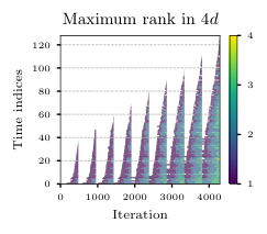
Figure 7. Norms of computed error estimates and error bounds in dependence on the iteration number for the heat equation with initial value, for d=4,8,16d=4,8,16.
Figure 8. Sum of the support and maximum rank per iteration versus the current residual norm estimate for the heat equation with initial value, for d=4,8,16d=4,8,16.
Refer to caption
Refer to caption
Refer to caption
Figure 9. Maximum ranks for each time index in dependence on the iteration number for the heat equation with initial value, for d=4,8,16d=4,8,16.
Refer to caption
Refer to caption
Refer to caption
Figure 10. Sum of one-dimensional support for each time index in dependence on the iteration number for the heat equation with initial value, for d=4,8,16d=4,8,16.
Figure 11. Time required for each inner iteration step for the heat equation with initial value for d=4,8,16d=4,8,16 in dependence on the achieved residual estimate.

In the following we present the same quantities as in Section 7.2.1. Figure 7 shows the residuals as well as the corresponding estimates for the 𝒳\mathcal{X}-norm with respect to the iteration number for the three different spatial dimensions d∈{4,8,16}d\in\{4,8,16\}, again with the expected behaviour. Figures 8, 9 and 10 show results for the one-dimensional supports as well as for the maximum ranks. Figure 8 compares the sum of the one-dimensional support with the computed residual norm estimates, where one can see that preasymptotic behaviour is still present. Figure 11 shows the time for each inner iteration step in dependence of the residual estimates for different spatial dimensions. As in the previous test case, we observe a polynomial dependence of the costs on the problem dimension. Altogether, the results are consistent with the previous test case with vanishing initial value. However, due to the higher computation costs, in the present case we do not enter the asymptotic regime for the one-dimensional support sizes.

8. Conclusion and Outlook

We have constructed a space-time adaptive solver for parabolic PDEs that combines sparse wavelet approximations in time with low-rank hierarchical tensor approximations in the spatial variables. The method yields guaranteed error bounds with respect to the exact solution in the natural norm of L2​(0,T,H01​(Ω))∩H1​(0,T,H−1​(Ω))L_{2}(0,T;H^{1}_{0}(\Omega))\cap H^{1}(0,T;H^{-1}(\Omega)). In addition, we obtain near-optimal bounds on hierarchical ranks and discretization sizes in terms of those of best approximations of similar accuracy, and corresponding bounds on the total computational complexity of the method in terms of the total error with respect to the exact solution of the PDE.

The present paper shows how such methods can be constructed and that they are applicable to problems in large dimensions dd. On this basis, there is a number of directions for further work. Concerning the quantitative efficiency of the method, based on the adaptive residual approximation constructed here, several further improvements are possible. In particular, the conceptually simple but quantitatively rather expensive approximate Richardson iteration on the full sequence space can be replaced by successively refined Galerkin discretizations as in [1]. For the arising Galerkin subproblems, solvers that are optimized for the particular structure of the combined sparse and low-rank approximations can be considered. Moreover, it will be of interest to adapt the method to convection-diffusion problems.

Another direction of future work concerns the approximability of solutions in the particular sense that is exploited by our adaptive scheme, especially in the case of large dd. On the one hand, the performance of the method depends on best nn-term approximations of the lower-dimensional contractions π(t,i)​(𝐮)\pi^{(\mathrm{t},i)}(\mathbf{u}) for i=1,…,di=1,\ldots,d; this can be interpreted as the approximability by adaptive tensor product wavelets of densities of solutions with respect to the temporal and a single spatial variable. On the other hand, the performance of the method depends on the ranks of spatial hierarchical low-rank approximations of the coefficient tensors 𝐮νt\mathbf{u}_{\nu_{\mathrm{t}}} for each fixed temporal basis index νt∈∨t\nu_{\mathrm{t}}\in\vee_{\mathrm{t}}.

Since our method does not make explicit use of any assumptions on approximability of solutions, but is guaranteed to automatically produce near-best approximations, it can be regarded as a numerical test for such approximability. Our numerical results show a (poly)logarithmic growth of hierarchical ranks with respect to the total solution error. This leads us to the conjecture that for parabolic problems of this type with data (such as initial values and source terms) having polylogarithmic growth of best approximation ranks, this polylogarithmic rank growth transfers to solutions. Such results have been obtained for elliptic problems in [19], but we are not aware of a comparable result for parabolic problems. Note that, as such exponential-type convergence of low-rank approximations is generally a structural feature of solutions, this is not covered by singular value decay estimates for generic elements of smoothness classes. For example, the estimates for functions with dominating mixed smoothness in [26, 10] yield only algebraic convergence with respect to ranks, which in view of the numerical results obtained here, and those for the elliptic case in [1, 8], is generally far from sharp for solutions of the considered PDE problems.

Appendix A Exponential Sum Approximations

In this section we give the proof of Theorem 4.1. The starting point for obtaining exponential sum approximations are integral representations based on the inverse Laplace transform. These are approximated in suitably transformed form by the trapezodial rule. We start with an auxiliary statement on the values of the derivative of the Dawson function on specific lines in the complex plane.

Lemma A.1.

One has

|1−2c(3±i)F(c(3±i))|≤1+2​πe+23xminF(xmin)≕cdaw\displaystyle\bigl\lvert 1-2c(\sqrt{3}\pm i)F\bigl(c(\sqrt{3}\pm i)\bigr)\bigr\rvert\leq 1+\sqrt{\frac{2\pi}{e}}+\frac{2}{\sqrt{3}}x_{\min}F(x_{\min})\eqqcolon c_{\mathrm{daw}}

for each c≥0c\geq 0, where xminx_{\min} is the global minimizer of d​Fd​x\frac{dF}{dx} [47].

Proof.

We will give the proof for the “+” case. The other case can be shown in the same way. Let c≥0c\geq 0 be arbitrary and set z=c⁡(3+i)z=c(\sqrt{3}+i). First, we start by estimating |F⁡(z)|\lvert F(z)\rvert. Choosing an axis-parallel contour, we have

∫0zeξ2​𝑑ξ\displaystyle\int\limits_{0}^{z}e^{\xi^{2}}d\xi =∫0Im⁡ze(i​y)2​𝑑y+∫0Re⁡ze(x+i​Im⁡(z))2​𝑑x\displaystyle=\int\limits_{0}^{\operatorname{Im}z}e^{(iy)^{2}}dy+\int\limits_{0}^{\operatorname{Re}z}e^{(x+i\operatorname{Im}(z))^{2}}dx
=π2​erf⁡(c)+e−c2​∫03​cex2​e2​i​c​x​𝑑x.\displaystyle=\frac{\sqrt{\pi}}{2}\operatorname{erf}(c)+e^{-c^{2}}\int\limits_{0}^{\sqrt{3}c}e^{x^{2}}e^{2icx}dx.

Using the definition of the Dawson function as well as the triangle inequality, we obtain

|F(z)|=|e−z2||∫0zeξ2dξ|≤e−2​c2π2erf(c)+F(3c).\lvert F(z)\rvert=\bigl\lvert e^{-z^{2}}\bigr\rvert\biggl\lvert\int\limits_{0}^{z}e^{\xi^{2}}d\xi\biggr\rvert\leq e^{-2c^{2}}\frac{\sqrt{\pi}}{2}\operatorname{erf}(c)+F(\sqrt{3}c).

We next take into account that the derivative of the Dawson function d​Fd​x=1−2​x​F\frac{dF}{dx}=1-2xF has its global minimum at xminx_{\min}. As a consequence,

|1−2​z​F​(z)|\displaystyle\lvert 1-2zF(z)\rvert ≤1+2​|z|​|F⁡(z)|\displaystyle\leq 1+2\lvert z\rvert\lvert F(z)\rvert
≤1+2​c​e−2​c2​π​erf⁡(c)+2​c​F​(3​c)\displaystyle\leq 1+2ce^{-2c^{2}}\sqrt{\pi}\operatorname{erf}(c)+2cF(\sqrt{3}c)
≤1+2​πe+23​xmin​F​(xmin)=cdaw.∎\displaystyle\leq 1+\sqrt{\frac{2\pi}{e}}+\frac{2}{\sqrt{3}}x_{\min}F(x_{\min})=c_{\mathrm{daw}}.\qed

We use the following definition and approximation error bound from [40].

Definition A.2.

For ζ>0\zeta>0, let Dζ={z∈ℂ:|Im​z|<ζ}D_{\zeta}=\{z\in\mathbb{C}:\lvert\mathrm{Im}\ z\rvert<\zeta\}, and for 0<ε<10<\varepsilon<1, let

Dζ(ε)={z∈ℂ:|Rez|<ε−1,|Imz|<ζ(1−ε)}.\displaystyle D_{\zeta}(\varepsilon)=\{z\in\mathbb{C}:\lvert\mathrm{Re}\ z\rvert<\varepsilon^{-1},\lvert\mathrm{Im}\ z\rvert<\zeta(1-\varepsilon)\}.

For vv analytic in DζD_{\zeta} let

N1​(v,Dζ)=limε→0∫∂Dζ​(ε)|v⁡(z)|​|𝑑z|.\displaystyle N_{1}(v,D_{\zeta})=\lim\limits_{\varepsilon\to 0}\int\limits_{\partial D_{\zeta}(\varepsilon)}\lvert v(z)\rvert\lvert\mathrm{d}z\rvert.
Theorem A.3 (see [40, Theorem 3.2.1]).

Let gg be analytic in DζD_{\zeta} with N1​(g,Dζ)<∞N_{1}(g,D_{\zeta})<\infty, then

|∫ℝg⁡(x)​𝑑x−h​∑k∈ℤg⁡(k​h)|≤e−πζ/h2​sinh⁡(π​ζ/h)​N1​(g,Dζ).\displaystyle\left\lvert\int_{\mathbb{R}}g(x)\,\mathrm{d}x-h\sum\limits_{k\in\mathbb{Z}}g(kh)\right\rvert\leq\frac{e^{-\pi\zeta/h}}{2\sinh(\pi\zeta/h)}N_{1}(g,D_{\zeta}).
Proof of Theorem 4.1.

Our starting point is the representation

ss+a~=∫0∞1π​y​(1−2​y​a​F​(y​a))​e−y​s​𝑑y,\displaystyle\frac{\sqrt{s}}{s+\tilde{a}}=\int\limits_{0}^{\infty}\frac{1}{\sqrt{\pi}\sqrt{y}}\Bigl(1-2\sqrt{ya}F\bigl(\sqrt{ya}\bigr)\Bigr)e^{-ys}\,\mathrm{d}y,

where we make use of the property d​Fd​x​(x)+2​x​F​(x)=1\frac{\mathrm{d}F}{\mathrm{d}x}(x)+2xF(x)=1 of the Dawson function FF given by (4.4). Substituting y​a=exya=e^{x} yields

ss+a\displaystyle\frac{\sqrt{s}}{s+a} =1a​π​∫ℝ(1−2​ex2​F​(ex2))​ex2−1a​ex​s​𝑑x\displaystyle=\frac{1}{\sqrt{a}\sqrt{\pi}}\int\limits_{\mathbb{R}}\left(1-2e^{\frac{x}{2}}F\left(e^{\frac{x}{2}}\right)\right)e^{\frac{x}{2}-\frac{1}{a}e^{x}s}\,\mathrm{d}x
=2​1a​π​∫ℝd​Fd​x​(ex/2)​e−1a​ex​s​𝑑x.\displaystyle=2\frac{1}{\sqrt{a}\sqrt{\pi}}\int\limits_{\mathbb{R}}\tfrac{dF}{dx}(e^{x/2})e^{-\frac{1}{a}e^{x}s}\,\mathrm{d}x.

The integrand is holomorphic in the strip {x+iy:x∈ℝ,|y|<π/3}\{x+iy:x\in\mathbb{R},\lvert y\rvert<\pi/3\}. In order to apply Theorem A.3, we need to estimate the quantity

N1​(g,Dζ)=∫ℝ|g⁡(x+i​ζ)|​𝑑x+∫ℝ|g⁡(x−i​ζ)|​𝑑x\displaystyle N_{1}(g,D_{\zeta})=\int_{\mathbb{R}}\lvert g(x+i\zeta)\rvert\,\mathrm{d}x+\int_{\mathbb{R}}\lvert g(x-i\zeta)\rvert\,\mathrm{d}x

where g⁡(x)=aπ​(1−2​ex/2​F​(ex/2))​ex2−1a​ex​sg(x)=\frac{\sqrt{a}}{\sqrt{\pi}}\left(1-2e^{x/2}F(e^{x/2})\right)e^{\frac{x}{2}-\frac{1}{a}e^{x}s}. By Lemma A.1, we have

|1−2​ex±y​i2​F​(ex±y​i2)|≤cdaw\displaystyle\left\lvert 1-2e^{\frac{x\pm yi}{2}}F\left(e^{\frac{x\pm yi}{2}}\right)\right\rvert\leq c_{\mathrm{daw}}

for y=π/3y=\pi/3 and all x∈ℝx\in\mathbb{R}. Moreover,

|ex+y​i2−1a​ex+y​i​t|\displaystyle\Bigl\lvert e^{\frac{x+yi}{2}-\frac{1}{a}e^{x+yi}t}\Bigr\rvert =eRe⁡(x+y​i2−1a​ex+y​i​t)\displaystyle=e^{\mathrm{Re}(\frac{x+yi}{2}-\frac{1}{a}e^{x+yi}t)}
=ex2−1a​ex​cos⁡(y)​t.\displaystyle=e^{\frac{x}{2}-\frac{1}{a}e^{x}\cos(y)t}.

The same transformation can be done for the negative imaginary part using cos⁡(y)=cos⁡(−y)\cos(y)=\cos(-y). Putting this together, for ζ∈(0,π3)\zeta\in(0,\frac{\pi}{3}), which ensures cos⁡(ζ)>0\cos(\zeta)>0, we obtain

N1​(g,Dζ)≤2​cdawa​π​∫ℝex2−1a​ex​cos⁡(ζ)​s​𝑑x=2​cdaws​cos⁡(ζ),N_{1}(g,D_{\zeta})\leq 2\frac{c_{\mathrm{daw}}}{\sqrt{a}\sqrt{\pi}}\int_{\mathbb{R}}e^{\frac{x}{2}-\frac{1}{a}e^{x}\cos(\zeta)s}\,\mathrm{d}x=\frac{2c_{\mathrm{daw}}}{\sqrt{s\ \cos(\zeta)}},

where we have used that π​erf⁡(c​ex/2)/c{\sqrt{\pi}\,\operatorname{erf}(\sqrt{c}\ e^{x/2})}/{\sqrt{c}} is the antiderivative of ex2−c​exe^{\frac{x}{2}-ce^{x}} for c>0c>0. Theorem A.3 now yields

|ss+a−∑k∈ℤha​wa​(k​ha)​e−αa​(k​ha)​s|\displaystyle\left\lvert\frac{\sqrt{s}}{s+a}-\sum\limits_{k\in\mathbb{Z}}h_{a}w_{a}(kh_{a})e^{-\alpha_{a}(kh_{a})s}\right\rvert ≤e−π23​ha2​sinh⁡(π23​ha)​2​cdaw​2​1s\displaystyle\leq\frac{e^{-\frac{\pi^{2}}{3h_{a}}}}{2\sinh(\frac{\pi^{2}}{3h_{a}})}2c_{\mathrm{daw}}\sqrt{2}\frac{1}{\sqrt{s}}
≤e−π23​ha2​sinh⁡(π23​ha)​10​(1+a)​ss+a≤δ​ss+a\displaystyle\leq\frac{e^{-\frac{\pi^{2}}{3h_{a}}}}{2\sinh(\frac{\pi^{2}}{3h_{a}})}10(1+a)\frac{\sqrt{s}}{s+a}\leq\delta\frac{\sqrt{s}}{s+a}

with the choice of hah_{a} in (4.5), where we have used s≥1s\geq 1 as well as 2​cdaw​2≤102c_{\mathrm{daw}}\sqrt{2}\leq 10 in the second line.

In the next step, we truncate the doubly infinite sum from above at the index na+n^{+}_{a} at cost of an maximum error of δ\delta. We use that

2c+1​e−c​ex​F​(ex/2)+π​cc+1​erf⁡(c​ex/2)\displaystyle\frac{2}{c+1}e^{-ce^{x}}F(e^{x/2})+\sqrt{\pi}\frac{\sqrt{c}}{c+1}\operatorname{erf}\bigl(\sqrt{c}e^{x/2}\bigr)

is the antiderivative of (1−2​ex2​F​(ex2))​ex2−c​ex(1-2e^{\frac{x}{2}}F(e^{\frac{x}{2}}))e^{\frac{x}{2}-ce^{x}}. Setting ua​(x)=wa​(x)​e−αa​(x)​su_{a}(x)=w_{a}(x)e^{-\alpha_{a}(x)s} and c=s/ac=s/a, we obtain

∑k>na+ha​ua​(k​ha)\displaystyle\sum\limits_{k>n^{+}_{a}}h_{a}u_{a}(kh_{a}) ≤∫na+∞ha​wa​(x​ha)​e−αa​(x​ha)​s​𝑑x=1π​a​∫na+​ha∞(1−2​ex2​F​(ex2))​ex2−c​ex​𝑑x\displaystyle\leq\int\limits_{n^{+}_{a}}^{\infty}h_{a}w_{a}(xh_{a})\,e^{-\alpha_{a}(xh_{a})s}\,\mathrm{d}x=\frac{1}{\sqrt{\pi}\sqrt{a}}\int\limits_{n^{+}_{a}h_{a}}^{\infty}\Bigl(1-2e^{\frac{x}{2}}F\bigl(e^{\frac{x}{2}}\bigr)\Bigr)e^{\frac{x}{2}-ce^{x}}\,\mathrm{d}x
=1π​a​(π​cc+1​erfc⁡(c​ena+​ha2)−2c+1​e−c​ena+​ha​F​(ena+​ha2))\displaystyle=\frac{1}{\sqrt{\pi}\sqrt{a}}\left(\sqrt{\pi}\frac{\sqrt{c}}{c+1}\operatorname{erfc}\Bigl(\sqrt{c}e^{\frac{n^{+}_{a}h_{a}}{2}}\Bigr)-\frac{2}{c+1}e^{-ce^{n^{+}_{a}h_{a}}}F\Bigl(e^{\frac{n^{+}_{a}h_{a}}{2}}\Bigr)\right)
≤ss+a​erfc⁡(1a​ena+​ha2)<δ​ss+a\displaystyle\leq\frac{\sqrt{s}}{s+a}\operatorname{erfc}\biggl(\frac{1}{\sqrt{a}}e^{\frac{n^{+}_{a}h_{a}}{2}}\biggr)<\delta\frac{\sqrt{s}}{s+a}

with na+n^{+}_{a} chosen according to (4.6). In the last line we use that the complementary error function erfc=1−erf\operatorname{erfc}=1-\operatorname{erf} is monotonically decreasing and s≥1s\geq 1.

Finally, we truncate the sum in the negative range of indices. To this end, we limit the interval of possible values of ss to [1,K][1,K] for a fixed K>1K>1. We make use of the fact that the antiderivative of (1−2​e−x2​F​(e−x2))​e−x2−c​e−x(1-2e^{-\frac{x}{2}}F(e^{-\frac{x}{2}}))e^{-\frac{x}{2}-ce^{-x}} for c>0c>0 is given by

−2c+1​e−c​e−x​F​(e−x2)−π​cc+1​erf⁡(c​e−x2).\displaystyle-\frac{2}{c+1}e^{-ce^{-x}}F\bigl(e^{-\frac{x}{2}}\bigr)-\sqrt{\pi}\frac{\sqrt{c}}{c+1}\operatorname{erf}\bigl(\sqrt{c}e^{-\frac{x}{2}}\bigr).

Setting c=s/ac=s/a as before, we arrive at

∑k<−nha​ua​(k​ha)\displaystyle\sum\limits_{k<-n}h_{a}u_{a}(kh_{a}) =∑k>nha​ua​(−k​ha)\displaystyle=\sum\limits_{k>n}h_{a}u_{a}(-kh_{a})
≤1π​a​∫n​ha∞(1−2​e−x2​F​(e−x2))​e−x2−c​e−x​𝑑x\displaystyle\leq\frac{1}{\sqrt{\pi}\sqrt{a}}\int\limits_{nh_{a}}^{\infty}\left(1-2e^{-\frac{x}{2}F\left(e^{-\frac{x}{2}}\right)}\right)e^{-\frac{x}{2}-ce^{-x}}\,\mathrm{d}x
=1π​a​(2c+1​e−c​e−n​ha​F​(e−n​ha2)+π​cc+1​erf⁡(c​e−n​ha2))\displaystyle=\frac{1}{\sqrt{\pi}\sqrt{a}}\left(\frac{2}{c+1}e^{-ce^{-nh_{a}}}F\bigl(e^{-\frac{nh_{a}}{2}}\bigr)+\sqrt{\pi}\frac{\sqrt{c}}{c+1}\operatorname{erf}\bigl(\sqrt{c}e^{-\frac{nh_{a}}{2}}\bigr)\right)
=ss+a​(erf⁡(sa​e−n​ha2)+2​as​π​e−sa​e−n​ha​F​(e−n​ha2))\displaystyle=\frac{\sqrt{s}}{s+a}\left(\operatorname{erf}\left(\frac{\sqrt{s}}{\sqrt{a}}e^{-\frac{nh_{a}}{2}}\right)+\frac{2\sqrt{a}}{\sqrt{s}\sqrt{\pi}}e^{-\frac{s}{a}e^{-nh_{a}}}F\left(e^{-\frac{nh_{a}}{2}}\right)\right)
=ss+a​fa​(s,n​ha).\displaystyle=\frac{\sqrt{s}}{s+a}f_{a}(s,nh_{a}).

If we assume that nn is chosen sufficiently large to ensure F(e−(nha)/2)e−(nha)/2<12F(e^{-(nh_{a})/2})e^{-(nh_{a})/2}<\frac{1}{2}, one can easily check that the function fa​(s,x)f_{a}(s,x) is monotonically decreasing in some interval s∈[0,z]s\in[0,z] and monotonically increasing in the remaining interval s∈(z,∞)s\in(z,\infty). We thus conclude that the maximum value of the function fa​(s,x)f_{a}(s,x) for a given xx and the time interval [1,K][1,K] has to be located at one of the boundary values. ∎

Appendix B Auxiliary proofs

Proof of Lemma 3.4.

For 𝐮∈ℓ2​(∨)\mathbf{u}\in\ell_{2}(\vee) and 𝗋∈ℛ∨t\mathsf{r}\in\mathcal{R}^{\vee_{\mathrm{t}}}, let P~𝐮,𝗋:ℓ2​(∨)→ℱ⁡(𝗋)\tilde{\mathrm{P}}_{\mathbf{u},\mathsf{r}}\colon\ell_{2}(\vee)\to\mathcal{F}(\mathsf{r}) be defined by

∥𝐮−P~𝐮,𝗋​𝐮∥=min𝐰∈ℱ⁡(𝗋)⁡∥𝐮−𝐰∥.\lVert\mathbf{u}-\tilde{\mathrm{P}}_{\mathbf{u},\mathsf{r}}\mathbf{u}\rVert=\min_{\mathbf{w}\in\mathcal{F}(\mathsf{r})}\lVert\mathbf{u}-\mathbf{w}\rVert.

The operator has the representation

P~𝐮,𝗋=∑νt∈∨t𝐄νt⊗P~x,𝐮νt,𝗋νt\tilde{\mathrm{P}}_{\mathbf{u},\mathsf{r}}=\sum\limits_{\nu_{\mathrm{t}}\in\vee_{\mathrm{t}}}\mathbf{E}_{\nu_{\mathrm{t}}}\otimes\tilde{\mathrm{P}}_{\mathrm{x},\mathbf{u}_{\nu_{\mathrm{t}}},\mathsf{r}_{\nu_{\mathrm{t}}}}

with 𝐄νt=𝐞νt⊺​𝐞νt\mathbf{E}_{\nu_{\mathrm{t}}}=\mathbf{e}_{\nu_{\mathrm{t}}}^{\intercal}\mathbf{e}_{\nu_{\mathrm{t}}} and where P~x,𝐮νt,𝗋νt:ℓ2(∨x)→ℋ(rνt)\tilde{\mathrm{P}}_{\mathrm{x},\mathbf{u}_{\nu_{\mathrm{t}}},\mathsf{r}_{\nu_{\mathrm{t}}}}\colon\ell_{2}(\vee_{\mathrm{x}})\to\mathcal{H}(r_{\nu_{\mathrm{t}}}) is the linear projection such that P~x,𝐮νt,𝗋νt​𝐮νt\tilde{\mathrm{P}}_{\mathrm{x},\mathbf{u}_{\nu_{\mathrm{t}}},\mathsf{r}_{\nu_{\mathrm{t}}}}\mathbf{u}_{\nu_{\mathrm{t}}} is a best approximation in ℋ⁡(𝗋νt)\mathcal{H}(\mathsf{r}_{\nu_{\mathrm{t}}}) as in [6, Lemma 1]. A direct consequence of this representation is that the operator P~𝐮,𝗋\tilde{\mathrm{P}}_{\mathbf{u},\mathsf{r}} is also a linear projection. According to Proposition 3.3, we obtain

∥𝐯−P𝗋¯​(𝐮,α​η)​𝐯∥\displaystyle\lVert\mathbf{v}-\mathrm{P}_{\bar{\mathsf{r}}(\mathbf{u},\alpha\eta)}\mathbf{v}\rVert ≤κP​inf𝐰∈ℱ​(𝗋¯​(𝐮,α​η))∥𝐯−𝐰∥\displaystyle\leq\kappa_{P}\inf_{\mathbf{w}\in\mathcal{F}(\bar{\mathsf{r}}(\mathbf{u},\alpha\eta))}\lVert\mathbf{v}-\mathbf{w}\rVert
≤κP​∥𝐯−P~𝐮,𝗋¯​(𝐮,α​η)​𝐯∥\displaystyle\leq\kappa_{P}\lVert\mathbf{v}-\tilde{\mathrm{P}}_{\mathbf{u},\bar{\mathsf{r}}(\mathbf{u},\alpha\eta)}\mathbf{v}\rVert
≤κP​(∥(𝐈−P~𝐮,𝗋¯​(𝐮,α​η))​(𝐯−𝐮)∥+∥𝐮−P~𝐮,𝗋¯​(𝐮,α​η)​𝐮∥)\displaystyle\leq\kappa_{P}\big(\lVert(\mathbf{I}-\tilde{\mathrm{P}}_{\mathbf{u},\bar{\mathsf{r}}(\mathbf{u},\alpha\eta)})(\mathbf{v}-\mathbf{u})\rVert+\lVert\mathbf{u}-\tilde{\mathrm{P}}_{\mathbf{u},\bar{\mathsf{r}}(\mathbf{u},\alpha\eta)}\mathbf{u}\rVert\big)
≤κP​(1+α)​η.\displaystyle\leq\kappa_{P}(1+\alpha)\eta.

By definition rank∞⁡(P^κP​(1+α)​η​(𝐯))\rank_{\infty}\bigl(\hat{\mathrm{P}}_{\kappa_{\mathrm{P}}(1+\alpha)\eta}(\mathbf{v})\bigr) is chosen minimally to archive the bound κ⁡(1+α)​η\kappa(1+\alpha)\eta, which yields (3.6). Furthermore, (3.5) is an immediate consequence of the triangle inequality. ∎

Proof of Theorem 3.13.

Combining (3.5) in Lemma 3.4 and the definition of the coarsening operator in (3.18) together with the triangle inequality yield relation (3.19).

The statements in (3.20) follow directly from Theorem 3.6. The additional coarsening operator can at most reduce the ranks and does not affect these estimates.

The main part is the proof of the estimates (3.21). We set 𝐰^=P^κP​(1+α)​η​(𝐯)\hat{\mathbf{w}}=\hat{\mathrm{P}}_{\kappa_{\mathrm{P}}(1+\alpha)\eta}(\mathbf{v}). Let N∈ℕN\in\mathbb{N} be minimal such that ∥𝐮−RΛ¯​(𝐮,N)​𝐮∥≤α​η\lVert\mathbf{u}-\mathrm{R}_{\bar{\Lambda}(\mathbf{u},N)}\mathbf{u}\rVert\leq\alpha\eta. Then

∥𝐰^−RΛ¯​(𝐮,N)​𝐰^∥\displaystyle\lVert\hat{\mathbf{w}}-\mathrm{R}_{\bar{\Lambda}(\mathbf{u},N)}\hat{\mathbf{w}}\rVert ≤∥(𝐈−RΛ¯​(𝐮,N))​(𝐮−𝐰^)∥+∥𝐮−RΛ¯​(𝐮,N)​𝐮∥\displaystyle\leq\lVert(\mathbf{I}-\mathrm{R}_{\bar{\Lambda}(\mathbf{u},N)})(\mathbf{u}-\hat{\mathbf{w}})\rVert+\lVert\mathbf{u}-\mathrm{R}_{\bar{\Lambda}(\mathbf{u},N)}\mathbf{u}\rVert
≤∥𝐮−𝐰^∥+∥𝐮−RΛ¯​(𝐮,N)​𝐮∥≤(1+κP​(1+α)+α)​η,\displaystyle\leq\lVert\mathbf{u}-\hat{\mathbf{w}}\rVert+\lVert\mathbf{u}-\mathrm{R}_{\bar{\Lambda}(\mathbf{u},N)}\mathbf{u}\rVert\leq(1+\kappa_{\mathrm{P}}(1+\alpha)+\alpha)\eta,

where we used Lemma 3.4 to bound the first summand on the right-hand side. Hence, by (3.17), we have

(B.1) ∥𝐰^−RΛ⁡(𝐰^,N)​𝐰^∥\displaystyle\lVert\hat{\mathbf{w}}-\mathrm{R}_{\Lambda(\hat{\mathbf{w}},N)}\hat{\mathbf{w}}\rVert ≤κC​∥𝐰^−RΛ¯​(𝐰^,N)​𝐰^∥\displaystyle\leq\kappa_{\mathrm{C}}\lVert\hat{\mathbf{w}}-\mathrm{R}_{\bar{\Lambda}(\hat{\mathbf{w}},N)}\hat{\mathbf{w}}\rVert
≤κC​∥𝐰^−RΛ¯​(𝐮,N)​𝐰^∥≤κC​(1+α)​(κP+1)​η.\displaystyle\leq\kappa_{\mathrm{C}}\lVert\hat{\mathbf{w}}-\mathrm{R}_{\bar{\Lambda}(\mathbf{u},N)}\hat{\mathbf{w}}\rVert\leq\kappa_{\mathrm{C}}(1+\alpha)(\kappa_{\mathrm{P}}+1)\eta.

Without loss of generality we may assume that N≥dN\geq d. Keeping the optimality (3.16) of the best coarsen operator in mind, property (3.9) yields

α​η<∥𝐮−RΛ⁡(𝐮,N−1)​𝐮∥\displaystyle\alpha\eta<\lVert\mathbf{u}-\mathrm{R}_{\Lambda(\mathbf{u},N-1)}\mathbf{u}\rVert ≤inf∑i#​Λ(t,i)≤N−1(∑i=1d‖π(t,i)​(𝐮)−RΛ(t,i)​π(t,i)​(𝐮)‖2)12\displaystyle\leq\inf\limits_{\sum_{i}\#\Lambda^{(t,i)}\leq N-1}\left(\sum\limits_{i=1}^{d}\left\lVert\pi^{(\mathrm{t},i)}(\mathbf{u})-\mathrm{R}_{\Lambda^{(t,i)}}\pi^{(\mathrm{t},i)}(\mathbf{u})\right\rVert^{2}\right)^{\frac{1}{2}}
≤∑i=1dinf#​Λ(t,i)≤(N−1)/d‖π(t,i)​(𝐮)−RΛ(t,i)​π(t,i)​(𝐮)‖\displaystyle\leq\sum\limits_{i=1}^{d}\inf\limits_{\#\Lambda^{(t,i)}\leq(N-1)/d}\left\lVert\pi^{(\mathrm{t},i)}(\mathbf{u})-\mathrm{R}_{\Lambda^{(t,i)}}\pi^{(\mathrm{t},i)}(\mathbf{u})\right\rVert
≤(N−1d)−s​∑i=1d∥π(t,i)​(𝐮)∥𝒜s\displaystyle\leq\left(\frac{N-1}{d}\right)^{-s}\sum\limits_{i=1}^{d}\lVert\pi^{(\mathrm{t},i)}(\mathbf{u})\rVert_{{\mathcal{A}}^{s}}
≤2s​(Nd)−s​∑i=1d∥π(t,i)​(𝐮)∥𝒜s.\displaystyle\leq 2^{s}\left(\frac{N}{d}\right)^{-s}\sum\limits_{i=1}^{d}\lVert\pi^{(\mathrm{t},i)}(\mathbf{u})\rVert_{{\mathcal{A}}^{s}}\,.

We note that by (B.1), the coarsening operator C^κC​(κP+1)​(1+α)​η\hat{\mathrm{C}}_{\kappa_{\mathrm{C}}(\kappa_{\mathrm{P}}+1)(1+\alpha)\eta} retains at most NN terms. We combine this fact with the previous estimate, which results in

(B.2) ∑i=1d#​supp⁡(π(t,i)​(𝐰η))≤N≤2​d​α−1s​η−1s​(∑i=1d∥π(t,i)​(𝐮)∥𝒜s)1s.\displaystyle\sum\limits_{i=1}^{d}\#\supp\left(\pi^{(\mathrm{t},i)}(\mathbf{w}_{\eta})\right)\leq N\leq 2d\alpha^{-\frac{1}{s}}\eta^{-\frac{1}{s}}\left(\sum\limits_{i=1}^{d}\lVert\pi^{(\mathrm{t},i)}(\mathbf{u})\rVert_{{\mathcal{A}}^{s}}\right)^{\frac{1}{s}}.

Hence the first statement in (3.21) is shown. Now let N^i=#​supp⁡(π(t,i)​(𝐮))\hat{N}_{i}=\#\supp(\pi^{(\mathrm{t},i)}(\mathbf{u})) for i=1,…,di=1,\dots,d and N^=∑iN^i\hat{N}=\sum_{i}\hat{N}_{i} . We may assume without loss of generality N^i>0\hat{N}_{i}>0 for i=1,…,di=1,\dots,d. Resolve (B.2) for η\eta and inserting into (3.19), we observe

(B.3) ∥𝐮−𝐰η∥≤N^−s​C​(α)​ds​∑i=1d∥π(t,i)​(𝐮)∥𝒜s\displaystyle\lVert\mathbf{u}-\mathbf{w}_{\eta}\rVert\leq\hat{N}^{-s}C(\alpha)d^{s}\sum\limits_{i=1}^{d}\lVert\pi^{(\mathrm{t},i)}(\mathbf{u})\rVert_{{\mathcal{A}}^{s}}

where C⁡(α)=2s​α−1​(1+κP​(1+α)+κC​(κP+1)​(1+α))C(\alpha)=2^{s}\alpha^{-1}(1+\kappa_{\mathrm{P}}(1+\alpha)+\kappa_{\mathrm{C}}(\kappa_{\mathrm{P}}+1)(1+\alpha)).

Let 𝐮^i\hat{\mathbf{u}}_{i} be the best N^i\hat{N}_{i}-term approximation to π(t,i)​(𝐮)\pi^{(\mathrm{t},i)}(\mathbf{u}), then by using the properties of Proposition 3.8 we observe

∥π(t,i)​(𝐰η)∥𝒜s\displaystyle\lVert\pi^{(\mathrm{t},i)}(\mathbf{w}_{\eta})\rVert_{{\mathcal{A}}^{s}} ≤2s​(∥𝐮^i∥𝒜s+∥𝐮^i−π(t,i)​(𝐰η)∥𝒜s)\displaystyle\leq 2^{s}\left(\lVert\hat{\mathbf{u}}_{i}\rVert_{{\mathcal{A}}^{s}}+\lVert\hat{\mathbf{u}}_{i}-\pi^{(\mathrm{t},i)}(\mathbf{w}_{\eta})\rVert_{{\mathcal{A}}^{s}}\right)
≤2s​(∥π(t,i)​(𝐮)∥𝒜s+(2​N^i)s​∥𝐮^i−π(t,i)​(𝐰η)∥)\displaystyle\leq 2^{s}\left(\lVert\pi^{(\mathrm{t},i)}(\mathbf{u})\rVert_{{\mathcal{A}}^{s}}+(2\hat{N}_{i})^{s}\lVert\hat{\mathbf{u}}_{i}-\pi^{(\mathrm{t},i)}(\mathbf{w}_{\eta})\rVert\right)
≤2s​(∥π(t,i)​(𝐮)∥𝒜s+(2​N^i)s​(∥𝐮^i−π(t,i)​(𝐮)∥+∥π(t,i)​(𝐮)−π(t,i)​(𝐰η)∥))\displaystyle\leq 2^{s}\left(\lVert\pi^{(\mathrm{t},i)}(\mathbf{u})\rVert_{{\mathcal{A}}^{s}}+(2\hat{N}_{i})^{s}\left(\lVert\hat{\mathbf{u}}_{i}-\pi^{(\mathrm{t},i)}(\mathbf{u})\rVert+\lVert\pi^{(\mathrm{t},i)}(\mathbf{u})-\pi^{(\mathrm{t},i)}(\mathbf{w}_{\eta})\rVert\right)\right)
≤2s​((1+2s)​∥π(t,i)​(𝐮)∥+(2​N^i)s​∥π(t,i)​(𝐮)−π(t,i)​(𝐰η)∥),\displaystyle\leq 2^{s}\left((1+2^{s})\lVert\pi^{(\mathrm{t},i)}(\mathbf{u})\rVert+(2\hat{N}_{i})^{s}\lVert\pi^{(\mathrm{t},i)}(\mathbf{u})-\pi^{(\mathrm{t},i)}(\mathbf{w}_{\eta})\rVert\right),

where we used that #​supp⁡(𝐮^i−π(t,i)​(𝐰η))≤2​N^i\#\supp(\hat{\mathbf{u}}_{i}-\pi^{(\mathrm{t},i)}(\mathbf{w}_{\eta}))\leq 2\hat{N}_{i} in the second line. As a consequence of the Cauchy-Schwarz inequality, we have the componentwise estimate

|πνt,νx(t,i)​(𝐮)−πνt,νx(t,i)​(𝐰η)|≤πνt,νx(t,i)​(𝐮−𝐰η),\displaystyle\lvert\pi^{(\mathrm{t},i)}_{\nu_{\mathrm{t}},\nu_{\mathrm{x}}}(\mathbf{u})-\pi^{(\mathrm{t},i)}_{\nu_{\mathrm{t}},\nu_{\mathrm{x}}}(\mathbf{w}_{\eta})\rvert\leq\pi^{(\mathrm{t},i)}_{\nu_{\mathrm{t}},\nu_{\mathrm{x}}}(\mathbf{u}-\mathbf{w}_{\eta}),

which yields

∥π(t,i)​(𝐮)−π(t,i)​(𝐰η)∥≤∥π(t,i)​(𝐮−𝐰η)∥=∥𝐮−𝐰η∥.\displaystyle\lVert\pi^{(\mathrm{t},i)}(\mathbf{u})-\pi^{(\mathrm{t},i)}(\mathbf{w}_{\eta})\rVert\leq\lVert\pi^{(\mathrm{t},i)}(\mathbf{u}-\mathbf{w}_{\eta})\rVert=\lVert\mathbf{u}-\mathbf{w}_{\eta}\rVert.

Combining this fact with (B.3), we obtain

∥π(t,i)​(𝐰η)∥𝒜s≤2s​(1+2s)​∥π(t,i)​(𝐮)∥𝒜s+2s​C​(α)​ds​N^−s​(2​N^i)s​(∑k=1d∥π(t,k)​(𝐮)∥𝒜s).\displaystyle\lVert\pi^{(\mathrm{t},i)}(\mathbf{w}_{\eta})\rVert_{{\mathcal{A}}^{s}}\leq 2^{s}(1+2^{s})\lVert\pi^{(\mathrm{t},i)}(\mathbf{u})\rVert_{{\mathcal{A}}^{s}}+2^{s}C(\alpha)d^{s}\hat{N}^{-s}(2\hat{N}_{i})^{s}\biggl(\sum\limits_{k=1}^{d}\lVert\pi^{(\mathrm{t},k)}(\mathbf{u})\rVert_{{\mathcal{A}}^{s}}\biggr).

Summing over i=1,…,di=1,\dots,d and noting that N^−s​∑i=1d(2​N^i)s≤2s​dmax⁡(0,1−s)\hat{N}^{-s}\sum\limits_{i=1}^{d}(2\hat{N}_{i})^{s}\leq 2^{s}d^{\max(0,1-s)}, we arrive at the second statement in (3.21). ∎

References

  • [1] M. Ali and K. Urban, HT-AWGM: a hierarchical Tucker-adaptive wavelet Galerkin method for high-dimensional elliptic problems, Adv. Comput. Math. 46 (2020), no. 4, Paper No. 59, 34.
  • [2] R. Andreev, Stability of sparse space-time finite element discretizations of linear parabolic evolution equations, IMA J. Numer. Anal. 33 (2013), no. 1, 242–260.
  • [3] by same author, Wavelet-in-time multigrid-in-space preconditioning of parabolic evolution equations, SIAM J. Sci. Comput. 38 (2016), no. 1, A216–A242.
  • [4] R. Andreev and C. Tobler, Multilevel preconditioning and low-rank tensor iteration for space-time simultaneous discretizations of parabolic PDEs, Numer. Linear Algebra Appl. 22 (2015), no. 2, 317–337.
  • [5] M. Bachmayr, Low-rank tensor methods for partial differential equations, Acta Numer. 32 (2023), 1–121. MR 4586820
  • [6] M. Bachmayr and W. Dahmen, Adaptive near-optimal rank tensor approximation for high-dimensional operator equations, Found. Comput. Math. 15 (2015), no. 4, 839–898.
  • [7] by same author, Adaptive low-rank methods for problems on Sobolev spaces with error control in L2{\rm L}_{2}, ESAIM Math. Model. Numer. Anal. 50 (2016), no. 4, 1107–1136.
  • [8] by same author, Adaptive low-rank methods: problems on Sobolev spaces, SIAM J. Numer. Anal. 54 (2016), no. 2, 744–796.
  • [9] M. Bachmayr, H. Eisenmann, E. Kieri, and A. Uschmajew, Existence of dynamical low-rank approximations to parabolic problems, Math. Comp. 90 (2021), no. 330, 1799–1830.
  • [10] M. Bachmayr, A. Nouy, and R. Schneider, Approximation by tree tensor networks in high dimensions: Sobolev and compositional functions, Pure and Applied Functional Analysis 8 (2023), 405–428.
  • [11] A. Barinka, Fast evaluation tools for adaptive wavelet schemes, Ph.D. thesis, RWTH Aachen, 2005.
  • [12] C. Beck, S. Becker, P. Grohs, N. Jaafari, and A. Jentzen, Solving the Kolmogorov PDE by means of deep learning, J. Sci. Comput. 88 (2021), no. 3, Paper No. 73, 28.
  • [13] T. Boiveau, V. Ehrlacher, A. Ern, and A. Nouy, Low-rank approximation of linear parabolic equations by space-time tensor Galerkin methods, ESAIM Math. Model. Numer. Anal. 53 (2019), no. 2, 635–658.
  • [14] N. Chegini and R. Stevenson, Adaptive wavelet schemes for parabolic problems: sparse matrices and numerical results, SIAM J. Numer. Anal. 49 (2011), no. 1, 182–212.
  • [15] H. Cho, D. Venturi, and G. E. Karniadakis, Numerical methods for high-dimensional probability density function equations, J. Comput. Phys. 305 (2016), 817–837.
  • [16] A. Cohen, W. Dahmen, and R. DeVore, Adaptive wavelet methods for elliptic operator equations: convergence rates, Math. Comp. 70 (2001), no. 233, 27–75.
  • [17] by same author, Adaptive wavelet methods. II. Beyond the elliptic case, Found. Comput. Math. 2 (2002), no. 3, 203–245.
  • [18] D. Conte, Dynamical low-rank approximation to the solution of parabolic differential equations, Appl. Numer. Math. 156 (2020), 377–384.
  • [19] W. Dahmen, R. DeVore, L. Grasedyck, and E. Süli, Tensor-sparsity of solutions to high-dimensional elliptic partial differential equations, Foundations of Computational Mathematics 16 (2016), no. 4, 813–874.
  • [20] R. Dautray and J.-L. Lions, Mathematical analysis and numerical methods for science and technology. Vol. 5, Springer-Verlag, Berlin, 1992, Evolution problems. I, With the collaboration of Michel Artola, Michel Cessenat and Hélène Lanchon, Translated from the French by Alan Craig.
  • [21] T. J. Dijkema, C. Schwab, and R. Stevenson, An adaptive wavelet method for solving high-dimensional elliptic PDEs, Constr. Approx. 30 (2009), no. 3, 423–455.
  • [22] S. V. Dolgov, B. N. Khoromskij, and I. V. Oseledets, Fast solution of parabolic problems in the tensor train/quantized tensor train format with initial application to the Fokker-Planck equation, SIAM J. Sci. Comput. 34 (2012), no. 6, A3016–A3038.
  • [23] G. C. Donovan, J. S. Geronimo, and D. P. Hardin, Orthogonal polynomials and the construction of piecewise polynomial smooth wavelets, SIAM J. Math. Anal. 30 (1999), no. 5, 1029–1056.
  • [24] Th. Führer and M. Karkulik, Space-time least-squares finite elements for parabolic equations, Comput. Math. Appl. 92 (2021), 27–36.
  • [25] G. Gantner and R. Stevenson, Further results on a space-time FOSLS formulation of parabolic PDEs, ESAIM Math. Model. Numer. Anal. 55 (2021), no. 1, 283–299.
  • [26] M. Griebel, H. Harbrecht, and R. Schneider, Low-rank approximation of continuous functions in sobolev spaces with dominating mixed smoothness, Mathematics of Computation 92 (2023), no. 342, 1729–1746.
  • [27] M. Griebel and D. Oeltz, A sparse grid space-time discretization scheme for parabolic problems, Computing 81 (2007), no. 1, 1–34.
  • [28] W. Hackbusch, Tensor spaces and numerical tensor calculus, Springer Series in Computational Mathematics, vol. 42, Springer, Heidelberg, 2012.
  • [29] W. Hackbusch and S. Kühn, A new scheme for the tensor representation, J. Fourier Anal. Appl. 15 (2009), no. 5, 706–722.
  • [30] Y. Kazashi, F. Nobile, and E. Vidličková, Stability properties of a projector-splitting scheme for dynamical low rank approximation of random parabolic equations, Numer. Math. 149 (2021), no. 4, 973–1024.
  • [31] S. Kestler, K. Steih, and K. Urban, An efficient space-time adaptive wavelet Galerkin method for time-periodic parabolic partial differential equations, Math. Comp. 85 (2016), no. 299, 1309–1333.
  • [32] O. Koch and C. Lubich, Dynamical low-rank approximation, SIAM J. Matrix Anal. Appl. 29 (2007), no. 2, 434–454.
  • [33] S. Larsson and M. Molteni, Numerical solution of parabolic problems based on a weak space-time formulation, Comput. Methods Appl. Math. 17 (2017), no. 1, 65–84.
  • [34] C. Lubich, T. Rohwedder, R. Schneider, and B. Vandereycken, Dynamical approximation by hierarchical Tucker and tensor-train tensors, SIAM J. Matrix Anal. Appl. 34 (2013), no. 2, 470–494.
  • [35] A. Metselaar, Handling wavelet expansions in numerical methods, Ph.D. thesis, University of Twente, 2002.
  • [36] N. Rekatsinas and R. Stevenson, An optimal adaptive tensor product wavelet solver of a space-time FOSLS formulation of parabolic evolution problems, Adv. Comput. Math. 45 (2019), no. 2, 1031–1066.
  • [37] Ch. Schwab and R. Stevenson, Space-time adaptive wavelet methods for parabolic evolution problems, Math. Comp. 78 (2009), no. 267, 1293–1318.
  • [38] Ch. Schwab and E. Süli, Adaptive Galerkin approximation algorithms for Kolmogorov equations in infinite dimensions, Stoch. Partial Differ. Equ. Anal. Comput. 1 (2013), no. 1, 204–239.
  • [39] O. Steinbach and H. Yang, Space-time finite element methods for parabolic evolution equations: discretization, a posteriori error estimation, adaptivity and solution, Space-time methods—applications to partial differential equations, Radon Ser. Comput. Appl. Math., vol. 25, De Gruyter, Berlin, 2019, pp. 207–248.
  • [40] F. Stenger, Numerical methods based on Sinc and analytic functions, Springer series in computational mathematics, Springer, New York, 1993.
  • [41] R. Stevenson, On the compressibility of operators in wavelet coordinates, SIAM Journal on Mathematical Analysis 35 (2004), no. 5, 1110–1132.
  • [42] R. Stevenson, R. van Venetië, and J. Westerdiep, A wavelet-in-time, finite element-in-space adaptive method for parabolic evolution equations, Adv. Comput. Math. 48 (2022), no. 3, Paper No. 17, 43.
  • [43] R. Stevenson and J. Westerdiep, Stability of Galerkin discretizations of a mixed space-time variational formulation of parabolic evolution equations, IMA J. Numer. Anal. 41 (2021), no. 1, 28–47.
  • [44] F. Tantardini and A. Veeser, The L2L^{2}-projection and quasi-optimality of galerkin methods for parabolic equations, SIAM Journal on Numerical Analysis 54 (2016), 317–340.
  • [45] T. von Petersdorff and Ch. Schwab, Numerical solution of parabolic equations in high dimensions, M2AN Math. Model. Numer. Anal. 38 (2004), no. 1, 93–127.
  • [46] E. Wasserstein and The OEIS Foundation Inc., The on-line encyclopedia of integer sequences, https://oeis.org/A133841, 2022.
  • [47] by same author, The on-line encyclopedia of integer sequences, https://oeis.org/A133843, 2022.