First-detection-time statistics in many-body quantum transport

Let us start with providing a general description of stroboscopic measurements Dhar et al. 2015a; Dhar et al. 2015b; Friedman et al. 2016; Friedman et al. 2017; Thiel et al. 2018; Yin et al. 2019; Liu et al. 2020; Thiel et al. 2020a; Thiel et al. 2020b; Kessler et al. 2021 in the density operator formalism. To this end, consider a general quantum state (irrespective of the exact physical scenario) described by the density operator $\rho$ and suppose that it is initially prepared in the subspace $\mathscr{H}_{\parallel}$ of the total Hilbert space $\mathscr{H}=\mathscr{H}_{\parallel}\oplus\mathscr{H}_{\perp}$. We consider its coherent evolution generated by the Hamiltonian $\mathcal{H}$ and ask for the time delay to successfully detect the state in the detection subspace $\mathscr{H}_{\perp}$ for the first time. Our strategy is to perform repetitive measurements after equidistant sampling times $\tau$, according to the binary projective-valued measurement $\{\mathcal{P}_{\perp},\mathcal{P}_{\parallel}\}$, where $\mathcal{P}_{\perp}$ and $\mathcal{P}_{\parallel}=$\mathrm{-}$\mathcal{P}_{\perp}$ project on $\mathscr{H}_{\perp}$ and $\mathscr{H}_{\parallel}$, respectively. We stop the protocol after the first successful detection in $\mathscr{H}_{\perp}$.

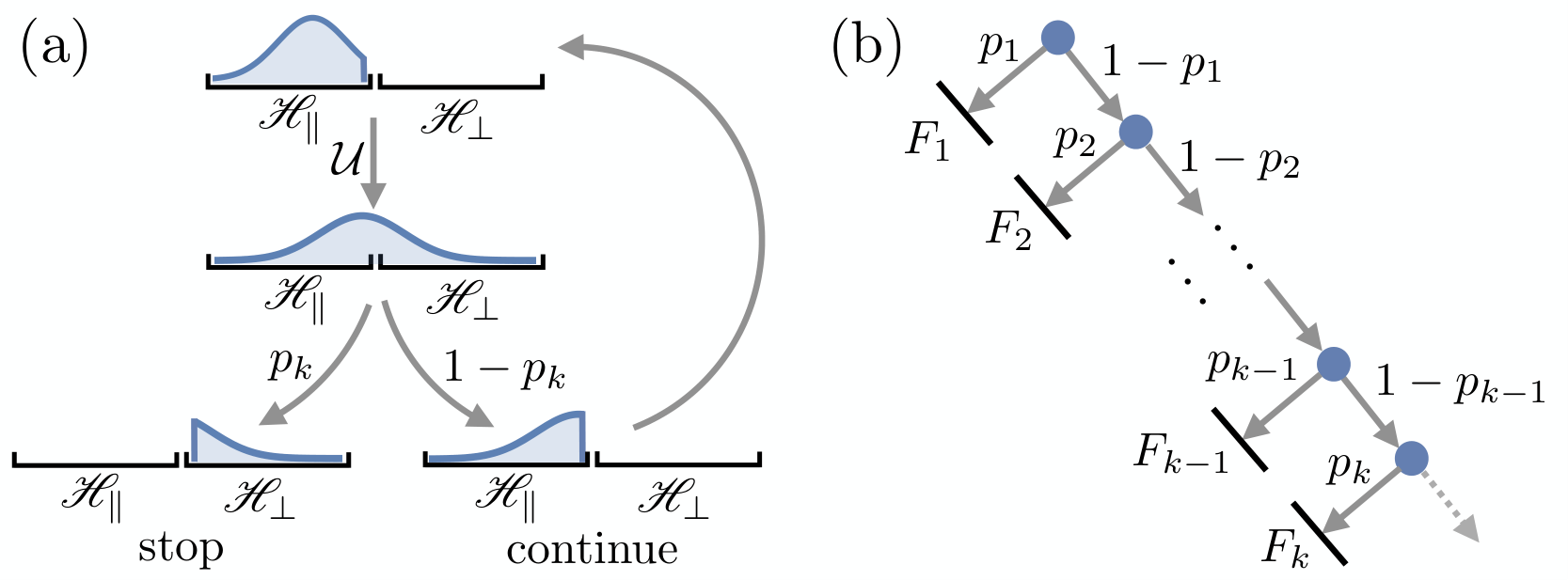
At the first measurement, the evolved state $\mathcal{U}\rho\mathcal{U}^{\dagger}$, with $\mathcal{U}=\exp(-\mathrm{i}\mathcal{H}\tau/\hbar)$, results in a successful detection with probability $p_{1}=\mathrm{Tr}\left(\mathcal{P}_{\perp}\mathcal{U}\rho\mathcal{U}^{\dagger}\mathcal{P}_{\perp}\right)$, causing the protocol to stop. In the case of an unsuccessful detection, the state has vanishing support on $\mathscr{H}_{\perp}$. It reduces to $\rho_{1}=\mathcal{P}_{\parallel}\mathcal{U}\rho\mathcal{U}^{\dagger}\mathcal{P}_{\parallel}/(1-p_{1})$ and continues evolving to $\mathcal{U}\rho_{1}\mathcal{U}^{\dagger}$ before the next measurement. By continuing in this way, illustrated in Fig. 1(a), the $k$th measurement yields a successful detection with probability

Hence, as evident from the tree diagram in Fig. 1(b), the probability for the first successful detection at the $k$th measurement, called first-detection probability, is $F_{k}=(1-p_{1})\cdots(1-p_{k-1})p_{k}$. Using Eq. (1) and the operator $\mathcal{T}_{k}=\mathcal{P}_{\perp}\mathcal{U}(\mathcal{P}_{\parallel}\mathcal{U})^{k-1}$, it reads

With this, the total detection probability after $k$ measurements is

and the survival probability, i.e., the probability for no successful detection after $k$ measurements, becomes

Since the stroboscopic measurement is performed with equidistant sampling times $\tau$, the first detection probabilities (2) allow us to define the first-detection time (sometimes called Friedman et al. 2017; Liu et al. 2020 mean first detection or passage time) as the expectation value of the detection time with respect to the probability distribution $\{F_{1}/D_{k},\dots,F_{k}/D_{k}\}$, in the limit of a large number $k$ of measurements,

Hence, the stroboscopic measurement protocol allows us to properly define the time after which we expect the first detection in the detection subspace $\mathscr{H}_{\perp}$.

The probabilities $F_{k}$, $D_{k}$, and $S_{k}$ are key for the first-detection-time statistics in stroboscopic measurements. They are further related through Eqs. (3) and (4) by

and thus serve equally well to obtain the full statistics of the first-detection times (5). Under this perspective, we can now focus on rewriting one of them, the survival probability $S_{k}$, in a more compact and intuitive form. To this end, let us introduce the block matrix representation

of a general linear operator $\mathcal{A}$ on $\mathscr{H}$, where the first (second) column and row corresponds to the subspace $\mathscr{H}_{\parallel}$ ($\mathscr{H}_{\perp}$). Accordingly, the projectors on these subspaces are $\mathcal{P}_{\parallel}=\mathrm{diag}($\mathrm{,}$0)$ and $\mathcal{P}_{\perp}=\mathrm{diag}(0,$\mathrm{)}$$ and the initial density matrix, which has vanishing support on the detection subspace $\mathscr{H}_{\perp}$, reads $\rho=\mathrm{diag}(\rho_{\parallel\parallel},0)$. As we show in Appendix A, we can express the survival probability (4) as the expectation value of the survival operator Dhar et al. 2015a; Dhar et al. 2015b

with respect to $\rho_{\parallel\parallel}$, that is,

Note that, as indicated by the decomposition (7), $\mathcal{U}_{\parallel\parallel}$ is the block of the unitary evolution operator $\mathcal{U}$ in the subspace $\mathscr{H}_{\parallel}$. Accordingly, we can intuitively interpret $S_{k}=\mathrm{Tr}(\mathcal{U}_{\parallel\parallel}^{k}\rho_{\parallel\parallel}(\mathcal{U}_{\parallel\parallel}^{k})^{\dagger})$ as the probability that the first $k$ measurements find the state in $\mathscr{H}_{\parallel}$, hence the probability for no successful detection after $k$ measurements.

From Eqs. (5), (6), (8), and (9), the first-detection-time statistics can be obtained by calculating the $k$th matrix power of the complex-valued matrix $\mathcal{U}_{\parallel\parallel}$ for all $k$. In general, $\mathcal{U}_{\parallel\parallel}$ is not a normal operator and hence cannot be diagonalized by a unitary matrix. However, it can be decomposed as $\mathcal{U}_{\parallel\parallel}=\mathcal{Q}\Lambda\mathcal{Q}^{-1}$ ¹¹ 1 Note that diagonalizable complex-valued matrices form a dense subset of the set of $n\times n$ complex matrices. Hence, almost all $n\times n$ complex matrices are diagonalizable and those which are not can be approximated to arbitrary precision by a diagonalizable matrix Horn and Johnson 2013., with the columns of $\mathcal{Q}$ corresponding to the not necessarily orthogonal eigenvectors of $\mathcal{U}_{\parallel\parallel}$ and $\Lambda=\mathrm{diag}(\lambda_{1},\lambda_{2},\dots)$ carrying the corresponding complex-valued eigenvalues on its diagonal. Consequently, given the diagonalization $\mathcal{U}_{\parallel\parallel}=\mathcal{Q}\Lambda\mathcal{Q}^{-1}$, the matrix power $\mathcal{U}_{\parallel\parallel}^{k}$ can efficiently be calculated via $\mathcal{U}_{\parallel\parallel}^{k}=\mathcal{Q}\Lambda^{k}\mathcal{Q}^{-1}$, with $\Lambda^{k}=\mathrm{diag}(\lambda_{1}^{k},\lambda_{2}^{k},\dots)$.

The eigenvalues $\lambda_{j}$ of $\mathcal{U}_{\parallel\parallel}$ are in general complex and satisfy $0\leq|\lambda_{j}|\leq 1$, where the upper bound is due to $S_{k}\leq 1$. From this we see that for increasing $k$, all eigenvalues $\lambda_{j}^{k}$ of $\mathcal{U}_{\parallel\parallel}^{k}$ for which $|\lambda_{j}|\neq 1$ vanish exponentially in $k$. Hence, in the limit $k\rightarrow\infty$, we are left with the subspace of $\mathcal{U}_{\parallel\parallel}$ spanned by the not necessarily orthogonal eigenvectors associated with the eigenvalues satisfying $|\lambda_{j}|=1$. Let us denote this subspace by $\mathscr{H}_{\mathrm{T}}$ and let $\mathcal{P}_{\mathrm{T}}$ be a projector on $\mathscr{H}_{\mathrm{T}}$. As we show in Appendix B, in the limit $k\rightarrow\infty$ we find that the survival operator $\lim_{k\rightarrow\infty}\mathcal{S}_{k}=\mathcal{S}_{\infty}$ projects on the subspace $\mathscr{H}_{\mathrm{T}}$, i.e.,

Accordingly, the survival probability $S_{\infty}=\mathrm{Tr}\left(\mathcal{P}_{\mathrm{T}}\rho_{\parallel\parallel}\right)$ is equivalent to the fraction of the initial state $\rho_{\parallel\parallel}$ living on $\mathscr{H}_{\mathrm{T}}$ and we therefore call $\mathscr{H}_{\mathrm{T}}$ the trapped subspace (note that in the literature Thiel et al. 2020a; Thiel et al. 2020b it is sometimes called dark subspace). That is, in the limit $k\rightarrow\infty$ there is a nonvanishing survival probability $S_{\infty}$ if and only if the initial state $\rho_{\parallel\parallel}$ has support on the trapped subspace $\mathscr{H}_{\mathrm{T}}$ (see also Thiel et al. 2020a; Thiel et al. 2020b).

We now continue with studying the convergence behavior of the first-detection time (5). First note that if $S_{\infty}=1$, the entire initial state remains in the trapped subspace and, from Eq. (5), $\braket{t_{\mathrm{f}}}$ is undefined. In the following we exclude this trivial case and consider $S_{\infty}<1$. As detailed in Appendix C, we first rewrite $\braket{t_{\mathrm{f}}}$ from Eq. (5) as

The convergence properties can then be investigated via the ratio test Hildebrandt 2006 of the series in (11). To this end, we consider the ratio

with the upper bound following from $S_{k+1}\leq S_{k}$. Since $\lim_{k\rightarrow\infty}S_{k}-S_{\infty}=0$, we naively expect $\braket{t_{\mathrm{f}}}$ from (11) to converge in the limit of a large number of measurements, $k\rightarrow\infty$. However, given a fixed but possibly large number of measurements $k$, it can happen that there is an additional limit in the sampling time, $\tau\rightarrow\tau_{\mathrm{res}}$, in which the ratio (12) becomes arbitrarily close to unity, hence indicating a divergent series in (11). Accordingly, the first-detection time (11) is then characterized by a competition between the limits $\tau\rightarrow\tau_{\mathrm{res}}$ and $k\rightarrow\infty$, which (as discussed below) can lead to a divergent (rather than convergent) behavior of $\braket{t_{\mathrm{f}}}$.

Such competition arises if there is at least one continuous, differentiable eigenvalue $\lambda_{j}(\tau)$ of $\mathcal{U}_{\parallel\parallel}$ (note that we explicitly state the dependence of $\lambda_{j}$ on the sampling time $\tau$), for which $\lim_{\delta\tau\rightarrow 0}|\lambda_{j}(\tau_{\mathrm{res}}\pm\delta\tau)|=1$, and $|\lambda_{j}(\tau_{\mathrm{res}}\pm\delta\tau)|<1$ for nonvanishing but small $\delta\tau$. We call these eigenvalues $\lambda_{j}(\tau)$ and sampling times $\tau_{\mathrm{res}}$ resonant eigenvalues and resonant sampling times, respectively. Then $\lim_{k\rightarrow\infty}|\lambda_{j}^{k}(\tau_{\mathrm{res}}\pm\delta\tau)|=0$ for nonvanishing $\delta\tau$ and $\lim_{\delta\tau\rightarrow 0}|\lambda_{j}^{k}(\tau_{\mathrm{res}}\pm\delta\tau)|=1$ for finite $k$.

Now note that the survival operator is Hermitian [see Eq. (8)] and, as we show in Appendix D, it can be written as $\mathcal{S}_{k}=\mathcal{P}_{\mathrm{T}}+\mathcal{M}_{k}$, where $\mathcal{P}_{\mathrm{T}}$ and $\mathcal{M}_{k}$ have orthogonal support, and $\lim_{k\rightarrow\infty}\mathcal{M}_{k}=0$. Further recall that $\mathcal{P}_{\mathrm{T}}$ [see Eq. (10)] projects on the trapped subspace $\mathscr{H}_{\mathrm{T}}$, which is spanned by the eigenvectors of $\mathcal{U}_{\parallel\parallel}$ associated with eigenvalues $|\lambda_{j}(\tau)|=1$. Hence, for $\delta\tau=0$ the eigenvalue $\lambda_{j}(\tau_{\mathrm{res}}\pm\delta\tau)$ is associated with $\mathcal{P}_{\mathrm{T}}$ and for $|\delta\tau|>0$ with $\mathcal{M}_{k}$. Therefore, $S_{k}$, and hence $\braket{t_{\mathrm{f}}}$, can be discontinuous at $\tau_{\mathrm{res}}$. We further conclude [recall that $\lambda_{j}(\tau)$ is continuous and differentiable] that the survival operator $\mathcal{S}_{k}$ must have an eigenvalue, which, for small $\delta\tau$, can be well approximated by $c_{m}^{(k)}\approx[1-\gamma(\delta\tau)^{2}]^{k}$, where $\gamma>0$. As we discuss in Appendix E, if the initial state $\rho_{\parallel\parallel}$ has nonvanishing support by the corresponding eigenvector $\ket{c_{m}^{(k)}}$ of $\mathcal{S}_{k}$, i.e., $\bra{c_{m}^{(k)}}\rho_{\parallel\parallel}\ket{c_{m}^{(k)}}\neq 0$, the first-detection time diverges for small $\delta\tau$ as

with $A,B>0$ approximately constant for small $\delta\tau$ [cf. Eqs. (47) and (52) in Liu et al. 2020].

Next let us see how the Hamiltonian’s spectral structure can lead to the appearance of resonant eigenvalues. To this end, consider the eigendecomposition $\mathcal{U}=\sum_{j}e^{-\mathrm{i}E_{j}\tau}|E_{j}\vphantom{E_{j}}\rangle\langle E_{j}\vphantom{E_{j}}|$ of the unitary evolution operator, with $\ket{E_{j}}$ the eigenvector associated with the eigenenergy $E_{j}$. Let us suppose nondegenerate eigenenergies $E_{j}$ and $\mathcal{P}_{\parallel}\ket{E_{j}}\neq\ket{E_{j}}$ [note that, if $\mathcal{P}_{\parallel}\ket{E_{j}}=\ket{E_{j}}$, then $\ket{E_{j}}$ is an eigenvector of $\mathrm{diag}(\mathcal{U}_{\parallel\parallel},0)$ whose associated eigenvalue $\lambda_{j}=e^{-\mathrm{i}E_{j}\tau}$ has unit modulus for any sampling time $\tau$. Degenerate eigenenergies $E_{j}$ can likewise lead to eigenvalues $\lambda_{j}$ with unit modulus for any sampling time $\tau$. However, these eigenvalues do not qualify as resonant eigenvalues as defined above]. Further suppose that there is a sampling time $\tau_{\Omega}$ and a corresponding set $\Omega$ of eigenenergies such that the eigenvalues $e^{-\mathrm{i}E_{j}\tau_{\Omega}}$ of $\mathcal{U}$ are degenerate for all $E_{j}\in\Omega$, i.e., Friedman et al. 2016; Friedman et al. 2017; Yin et al. 2019; Liu et al. 2020; Thiel et al. 2020b

We then call $\tau_{\Omega}$ the degenerate sampling time and define the corresponding degenerate subspace $\mathscr{H}_{\Omega}\subseteq\mathscr{H}$ spanned by the eigenvectors $\{\ket{E_{j}}\}_{E_{j}\in\Omega}$, with $\mathcal{P}_{\Omega}=\sum_{E_{j}\in\Omega}|E_{j}\vphantom{E_{j}}\rangle\langle E_{j}\vphantom{E_{j}}|$ projecting on $\mathscr{H}_{\Omega}$. As we show in detail in Appendix F, any vector $\ket{\lambda_{j}}\in\mathscr{H}$, which lives in the intersection of $\mathscr{H}_{\Omega}$ and $\mathscr{H}_{\parallel}$, i.e., $\mathcal{P}_{\Omega}\ket{\lambda_{j}}=\mathcal{P}_{\parallel}\ket{\lambda_{j}}=\ket{\lambda_{j}}$, constitutes an eigenvector of $\mathrm{diag}(\mathcal{U}_{\parallel\parallel},0)$ with associated eigenvalue $e^{-\mathrm{i}E_{\Omega}\tau_{\Omega}}$. Since $\ket{\lambda_{j}}\in\mathscr{H}$ has vanishing support on $\mathscr{H}_{\perp}$, i.e. $\mathcal{P}_{\perp}\ket{\lambda_{j}}=0$, we can drop the subspace $\mathscr{H}_{\perp}$ such that $\ket{\lambda_{j}}\in\mathscr{H}_{\parallel}$ becomes an eigenvector of $\mathcal{U}_{\parallel\parallel}$ whose associated eigenvalue $e^{-\mathrm{i}E_{\Omega}\tau_{\Omega}}$ has unit modulus and hence constitutes a resonant eigenvalue (see Appendix F for details). As a result, we showed that a degenerate sampling time can cause a resonant sampling time.

Let us now apply the above formalism of stroboscopic measurements to the quantum transport of $N$ identical particles evolving across a network composed of $l$ sites and investigate how (partial) particle distinguishability affects the first-detection-time statistics via many-particle interference. As a paradigmatic setting, we consider the particles to be initially prepared on the first $N$ sites ²² 2 Note that the more the particles initially bunch, the less there can be many-particle interference Dittel 2019; Dittel et al. 2021. Hence, we choose one particle per site to allow for strong interference effects. and a detection on site $l>N$, also called the target site. Note that we impose no restrictions on the particles’ hopping dynamics and on the position dependence of their mutual interaction; we merely suppose the dynamics to be governed by a general many-body unitary evolution matrix $\mathcal{U}$. As an example, which is numerically investigated in Sec. II.2 below, one can think of a linear lattice with nearest-neighbor coupling as illustrated in Fig. 2.

The Hilbert space $\mathscr{H}=\mathscr{H}_{\parallel}\oplus\mathscr{H}_{\perp}=\mathscr{H}_{1\mathrm{p}}^{\otimes N}$ is spanned by $N$-fold tensor products $\ket{\mathcal{E}_{1}}\otimes\dots\otimes\ket{\mathcal{E}_{N}}\equiv\ket{\mathcal{E}_{1}\cdots\mathcal{E}_{N}}$ of the single-particle basis states $\{\ket{\mathcal{E}_{j}}\}_{\mathcal{E}_{j}=1}^{l}$ of $\mathscr{H}_{1\mathrm{p}}$, with $\ket{\mathcal{E}_{j}}$ describing a single particle on site $\mathcal{E}_{j}$. For the initial state of one particle in each of the first $N$ sites, we have $\vec{\mathcal{E}}=(\mathcal{E}_{1}\cdots\mathcal{E}_{N})=(1\cdots N)$. Note that the case of bunched initial states can straightforwardly be described following Refs. Dittel 2019; Dittel et al. 2021.

Particle distinguishability is accounted for by additional internal degrees of freedom on an $N$-particle Hilbert space $\mathscr{H}_{\mathrm{int}}$. We make no restrictions on the particles’ nonsymmetrized internal states, described by a density operator $\sigma$ on $\mathscr{H}_{\mathrm{int}}$ (e.g., a pure product state gives $\sigma=\ket{\vec{\phi}}\bra{\vec{\phi}}$, with $\ket{\vec{\phi}}=\ket{\phi_{1}}\otimes\cdots\otimes\ket{\phi_{N}}$).

The initial state $\rho$ on $\mathscr{H}$ of $N$ partially distinguishable bosons (fermions) is then obtained by (anti)symmetrizing $|\vec{\mathcal{E}}\vphantom{\vec{\mathcal{E}}}\rangle\langle\vec{\mathcal{E}}\vphantom{\vec{\mathcal{E}}}|\otimes\sigma$ on $\mathscr{H}\otimes\mathscr{H}_{\mathrm{int}}$ with respect to all elements $\pi\in\mathrm{S}_{N}$ of the symmetric group $\mathrm{S}_{N}$ of $N$ elements and tracing over the particles’ internal degrees of freedom. Using the shorthand notation $\Pi_{\pi}\ket{\vec{\mathcal{E}}}=\ket{\vec{\mathcal{E}}_{\pi}}=\ket{\mathcal{E}_{\pi(1)}\cdots\mathcal{E}_{\pi(N)}}$, with permutations $\pi\in\mathrm{S}_{N}$, and $\Pi_{\pi}$ the corresponding permutation operator, this yields Dittel 2019; Minke et al. 2021; Dittel et al. 2021

with

Here $(-1)^{\pi\pi^{\prime}}_{\mathrm{B}}=1$ for bosons, $(-1)^{\pi\pi^{\prime}}_{\mathrm{F}}=\mathrm{sgn}(\pi\pi^{\prime})$ for fermions, and $\Pi_{\pi}$ permutes $\ket{\vec{\phi}}\in\mathscr{H}_{\mathrm{int}}$ similarly to $\ket{\vec{\mathcal{E}}}\in\mathscr{H}$. For perfectly indistinguishable particles, $\rho$ is pure and has maximal many-body coherences, i.e., off-diagonal elements, $\rho=|\psi_{\mathrm{B(F)}}\vphantom{\psi_{\mathrm{B(F)}}}\rangle\langle\psi_{\mathrm{B(F)}}\vphantom{\psi_{\mathrm{B(F)}}}|$, with $\ket{\psi_{\mathrm{B(F)}}}=(1/\sqrt{N!})\sum_{\pi\in\mathrm{S}_{N}}(-1)^{\pi}_{\mathrm{B(F)}}\ket{\vec{\mathcal{E}}_{\pi}}$ the usual pure state of $N$ indistinguishable bosons (fermions). On the other hand, for fully distinguishable particles we have $\rho_{\pi,\pi^{\prime}}=\delta_{\pi,\pi^{\prime}}/N!$. This yields a maximally mixed state $\rho=(1/N!)\sum_{\pi\in\mathrm{S}_{N}}|\vec{\mathcal{E}}_{\pi}\vphantom{\vec{\mathcal{E}}_{\pi}}\rangle\langle\vec{\mathcal{E}}_{\pi}\vphantom{\vec{\mathcal{E}}_{\pi}}|$, which is fully incoherent Dittel 2019; Dittel et al. 2021.

The coherences of $\rho$ are essential for many-particle interference in the particles’ transport dynamics. Hence, they are relevant for the first-detection-time statistics in stroboscopic measurements as directly apparent from Eq. (9). To this end, let us quantify the many-body coherences of $\rho$ via the expectation value of the projector $\Pi_{\mathrm{S}}=(1/N!)\sum_{\pi\in\mathrm{S}_{N}}\Pi_{\pi}$ on the symmetric subspace Minke et al. 2021; Brunner et al. 2022,

It corresponds to a sum of all elements of $\rho$ and satisfies $0\leq\braket{\Pi_{\mathrm{S}}}\leq 1$. The upper bound saturates for a fully symmetric state (e.g., fully indistinguishable bosons), the lower bound is reached if $\rho$ has no support on the symmetric subspace (e.g., if two or more fermions are fully indistinguishable), and fully distinguishable particles, which give rise to a fully incoherent state, result in $\braket{\Pi_{\mathrm{S}}}=1/N!$.

For the stroboscopic measurement, we consider different binary projective measurements: the detection of exactly $n$ ($=n$), and at least $n$ ($\geq n$) particles at the target site. As we show in Appendix G, the projectors on the corresponding detection subspaces can be expressed as

and

with $\mathcal{P}_{q}$ a genuine $q$-particle observable given by

Here $\mathcal{A}_{1}=|l\vphantom{l}\rangle\langle l\vphantom{l}|$, $\mathcal{A}_{2}=$$$, $L_{j}^{(q)}$ is the $j$th entry of the multiset ³³ 3 A multiset is a generalization of a set where multiple instances of the same element are allowed. $L^{(q)}=\{1\}^{q}\cup\{2\}^{N-q}$, and $\Sigma(L^{(q)})\subseteq\mathrm{S}_{N}$ is the right transversal ⁴⁴ 4 A transversal of a collection of sets $B_{1},\dots,B_{R}$ is a set of $R$ elements which contains exactly one element of each set $B_{1},\dots,B_{R}$. For $H$ a subgroup of the group $G$, the right transversal of $H$ in $G$ is a transversal of the set of distinct right cosets of $H$ in $G$. The right coset of $H$ in $G$ with respect to $\pi\in H$ is $H\pi=\{\xi\pi\ |\ \xi\in H\}$ Baumslag and Chandler 1968. of the Young subgroup $\mathrm{S}_{q}\otimes\mathrm{S}_{N-q}$ in $\mathrm{S}_{N}$ containing all ${N\choose q}$ permutations $\sigma$, which lead to distinctly ordered multisets. For example, for $N=2$ particles, we have the one-particle observable $\mathcal{P}_{1}=|l\vphantom{l}\rangle\langle l\vphantom{l}|\otimes$\mathrm{+}$$\otimes$|l\vphantom{l}\rangle\langle l\vphantom{l}|$ and the two-particle observable $\mathcal{P}_{2}=|l\vphantom{l}\rangle\langle l\vphantom{l}|\otimes|l\vphantom{l}\rangle\langle l\vphantom{l}|$. The projection operators on the detection subspaces can then be expressed as $\mathcal{P}^{=1}_{\perp}=\mathcal{P}_{1}-2\mathcal{P}_{2}=|l\vphantom{l}\rangle\langle l\vphantom{l}|\otimes($\mathrm{-}$|l\vphantom{l}\rangle\langle l\vphantom{l}|)+($\mathrm{-}$|l\vphantom{l}\rangle\langle l\vphantom{l}|)\otimes|l\vphantom{l}\rangle\langle l\vphantom{l}|$, $\mathcal{P}^{=2}_{\perp}=\mathcal{P}_{2}$, and $\mathcal{P}^{\geq 1}_{\perp}=\mathcal{P}_{1}-\mathcal{P}_{2}=\mathcal{P}^{=1}_{\perp}+\mathcal{P}^{=2}_{\perp}$. A comparison of Eqs. (19) and (20) shows that both expressions merely differ by the fraction $n/q$ in (20). Since $\mathcal{P}_{q}$ is a genuine $q$-particle observable and this fraction decreases for increasing $q$, we see that the sensitivity of $\mathcal{P}^{\geq n}_{\perp}$ to genuine $q$-particle effects (e.g., $q$-particle interference) decreases for increasing $q$ as compared to $\mathcal{P}^{=n}_{\perp}$. Hence, in accordance with the typical interpretation of (anti)bunching as a manifestation of many-particle properties Carolan et al. 2014; Shchesnovich 2016, for the measurement $\mathcal{P}^{=n}_{\perp}$ we expect more pronounced many-particle interference effects in the first-detection-time statistics compared to $\mathcal{P}^{\geq n}_{\perp}$.

The stroboscopic measurement corresponding to the detection of a fully bunched event on the target site, i.e., the detection of exactly $N$ particles with projector $\mathcal{P}^{=N}_{\perp}$, is particularly interesting. In this case, we find that the first-detection probability (2) is weighted by the fraction (17) of $\rho$ on the symmetric subspace. In particular, as we show in Appendix H, we find

with $F_{k}^{\mathrm{D}}$ the first-detection probability in the case of fully distinguishable particles. Accordingly, the total detection probability (3) becomes $D_{k}=N!\braket{\Pi_{\mathrm{S}}}D_{k}^{\mathrm{D}}$ and the survival probability (4)

Using this for the first-detection time $\braket{t_{\mathrm{f}}}$ in Eq. (5), we see that the factor $N!\braket{\Pi_{\mathrm{S}}}$ cancels such that $\braket{t_{\mathrm{f}}}$ is independent on the particles’ distinguishability, i.e.,

with $\braket{t_{\mathrm{f}}^{\mathrm{D}}}$ the first-detection time for fully distinguishable particles. However, note that $\braket{t_{\mathrm{f}}}$ is undefined if $\braket{\Pi_{\mathrm{S}}}=0$ since then $D_{\infty}=0$ [cf. Eq. (5)]. This, for example, applies to two or more fully indistinguishable fermions, as a consequence of Pauli’s exclusion principle, which prohibits the detection of indistinguishable fermions on the same site.

We now turn to the numerical investigation of an example for the above-described stroboscopic measurements in many-particle quantum transport. To this end we consider $N=2$ noninteracting, partially distinguishable particles initially prepared in the first two sites of a linear lattice with $l>N$ sites (see Fig. 2). We suppose nearest-neighbor tunneling, with equal tunneling rates between neighboring sites, and ask for the first-detection time to detect at least one ($\geq 1$), exactly one ($=1$), and exactly two ($=2$) particles at the target site $l$.

For the particles’ internal state we consider a pure product state $\ket{\vec{\phi}}=\ket{\phi_{1}}\otimes\ket{\phi_{2}}\in\mathscr{H}_{\text{int}}$, with $\ket{\phi_{j}}$ the internal state of the $j$th particle such that, after (anti)symmetrization, the initial state (15) reads

with the upper (lower) sign corresponding to bosons (fermions). Note that the particles’ indistinguishability is encoded in the off-diagonal entries of $\rho$ and quantified by the expectation value of the projector on the symmetric subspace (18), yielding $\braket{\Pi_{\mathrm{S}}}=(1\pm\left|\langle\phi_{1}\vphantom{\phi_{2}}|\phi_{2}\vphantom{\phi_{1}}\rangle\right|^{2})/2$.

The linear lattice with constant tunneling rate $J$ between neighboring sites is described by the single-particle Hamiltonian

which generates the single-particle unitary evolution operator $\mathcal{U}_{1\mathrm{p}}=\exp(-\mathrm{i}\mathcal{H}_{1\mathrm{p}}\tau/\hbar)$. Since we consider noninteracting particles, the two-particle unitary evolution operator is obtained from the tensor power thereof, $\mathcal{U}=\mathcal{U}_{1\mathrm{p}}^{\otimes 2}$.

With the two-particle unitary evolution operator $\mathcal{U}$ and the initial two-particle state $\rho$ at hand, we calculate the moduli of the eigenvalues of $\mathcal{U}_{\parallel\parallel}$, the survival probability $S_{\infty}$, and the first-detection time $\braket{t_{\mathrm{f}}}$ [using Eqs. (9)-(11)] for $501$ equally spaced sampling times in the interval $0\leq\tau J/\hbar\leq 10$ as well as for all resonant sampling times, nine different particle distinguishabilities equally spaced in the interval $-1\leq\pm\left|\langle\phi_{1}\vphantom{\phi_{2}}|\phi_{2}\vphantom{\phi_{1}}\rangle\right|^{2}\leq 1$, and different lattice lengths $l=3,\ 5,\ 7,$ and $10$. In our calculation of the first-detection time, the sum in Eq. (11) is truncated if $S_{k}-S_{\infty}<10^{-4}$ or $k>10^{4}$ due to limited computation time. In the vicinity of divergences of the first-detection time $\braket{t_{\mathrm{f}}}$, this truncation as well as the finite resolution of the sampling time may result in a peak instead of a true divergence to infinity [for example, in Fig. 3(p)].

Let us start by discussing the linear lattice with $l=3$ sites. In this particular case, the particles’ dynamics are perfectly periodic for sampling times $\tau J/\hbar$, which are integer multiples of $2\pi/\sqrt{2}\approx 4.44$, i.e., for $\tau J/\hbar=z2\pi/\sqrt{2}$, with $z\in\mathbb{N}_{0}$, we have $\mathcal{U}=$$$. As a result, we see a periodic behavior for the moduli $\left|\lambda_{j}\right|$ of the eigenvalues of $\mathcal{U}_{\parallel\parallel}$ in Figs. 3(a)-3(c). Here resonant eigenvalues with associated resonant sampling times $\tau_{\mathrm{res}}$ are marked by closed circles. As discussed in detail in Sec. I.4, depending on the initial state, the first-detection time $\braket{t_{\mathrm{f}}}$ can diverge for these resonant sampling times. This is evident by comparing the resonant sampling times in Figs. 3(a)-3(c) with the divergences of the first-detection time in Figs. 3(g)-3(i). Note that for the measurement of at least one and exactly one particle at the target site, the divergences of $\braket{t_{\mathrm{f}}}$ in Figs. 3(g) and 3(h) only appear if $\tau J/\hbar$ is an integer multiple of $2\pi/\sqrt{2}$. These are the sampling times for which $\mathcal{U}=$$$ due to the periodic dynamics, with all eigenvalues of $\mathcal{U}_{\parallel\parallel}$ satisfying $\left|\lambda_{j}\right|=1$ [see Figs. 3(a) and 3(b)]. Accordingly, for these sampling times the initial state remains unaffected such that nothing can be detected at the target site, as indicated by the survival probability $S_{\infty}=1$ in Figs. 3(d) and 3(e). In the vicinity of these sampling times, the unitary evolution operator slightly deviates from the identity. As a result, the divergence of $\braket{t_{\mathrm{f}}}$ at these sampling times can be understood through the quantum Zeno effect Degasperis et al. 1974.

For the measurement of exactly two particles at the target site, there are additional divergences of $\braket{t_{\mathrm{f}}}$ for resonant sampling times, which are no integer multiples of $2\pi/\sqrt{2}$ [see Fig. 3(i)]. These divergences can be understood through the competition of the limits $\delta\tau\rightarrow 0$ and $k\rightarrow\infty$ in the vicinity of resonant eigenvalues $\lambda_{j}^{k}(\tau_{\mathrm{res}}\pm\delta\tau)$ (see Sec. I.4). First consider the divergences appearing halfway between the periodic sampling times, at $\tau J/\hbar=(z+1/2)2\pi/\sqrt{2}$, with $z\in\mathbb{N}_{0}$, i.e., for $\tau J/\hbar\approx 2.22,6.66,\dots$. For these sampling times, the unitary evolution operator mirrors the initial state of the particles with respect to the second site such that one particle occupies site $2$ and one particle site $3$. This state has no support on the detection subspace for the measurement of exactly two particles at the target site. Hence, we have a unit survival probability $S_{\infty}=1$ [see Fig. 3(f)] and the first-detection time at these sampling times is undefined [see above Eq. (11)]. However, for small nonvanishing $\delta\tau$ around these sampling times, the state is not perfectly mirrored between consecutive measurements. In this case, $\braket{t_{\mathrm{f}}}$ is well defined and must diverge in the limit $\delta\tau\rightarrow 0$ for which the survival probability $S_{\infty}$ becomes unity. On the other hand, at the divergences which are not exactly halfway between periodic sampling times, e.g., for $\tau J/\hbar\approx 1.11,1.48,\dots$, the survival probability $S_{\infty}$ in Fig. 3(f) becomes unity only for perfectly indistinguishable fermions (which is due to Pauli’s exclusion principle). As a result, except for indistinguishable fermions, the first-detection time $\braket{t_{\mathrm{f}}}$ takes a finite value at these resonant sampling times, indicated by the closed circles in Fig. 3(i).

Next let us consider the effect of particle distinguishability for the survival probability $S_{\infty}$ and the first-detection time $\braket{t_{\mathrm{f}}}$ shown in Figs. 3(d)-3(i). First, consider the measurement of exactly two particles. In this case, we see that the survival probability shown in Fig. 3(f) follows Eq. (23), which for the two-particle state (25) becomes $S_{k}=S_{k}^{\mathrm{D}}\mp\left|\langle\phi_{1}\vphantom{\phi_{2}}|\phi_{2}\vphantom{\phi_{1}}\rangle\right|^{2}(1-S_{k}^{\mathrm{D}})$, with the upper (lower) sign corresponding to bosons (fermions). Furthermore, as predicted by Eq. (24), Fig. 3(i) reveals that the first-detection time $\braket{t_{\mathrm{f}}}$ appears independently of the particles’ indistinguishability. For the measurement of at least one and exactly one particle at the target site, Figs. 3(d) and 3(e) show a vanishing survival probability $S_{\infty}=0$, independently of the particles’ distinguishability, except at integer multiples of the period $2\pi/\sqrt{2}$. However, between the divergences, the first-detection times in Figs. 3(g) and 3(h) show a clear dependence on the particles’ indistinguishability: The more symmetric the two-particle state, i.e., the larger $\pm\left|\langle\phi_{1}\vphantom{\phi_{2}}|\phi_{2}\vphantom{\phi_{1}}\rangle\right|^{2}$ in (25), the larger the first detection time $\braket{t_{\mathrm{f}}}$ ⁵⁵ 5 Note that an increasing first-detection time for increasing symmetry of the many-body state is not a generally valid trend. Instead, it is an artifact of the chosen lattice Hamiltonian. For example, for a one-dimensional linear lattice with three sites and periodic boundary conditions, i.e., for a ring, and for the detection of exactly one particle, we find sampling times for which the first-detection time increases with decreasing symmetry of the two-body state Neubrand 2020.. As expected from our considerations below Eq. (21), this effect appears more pronounced for the measurement of exactly one particle compared to the measurement of at least one particle.

Next we increase the lattice length to $l=5$ sites. The numerical results are shown in Figs. 3(j)-3(r). In this case, there are no perfectly periodic dynamics such that the survival probability yields $S_{\infty}=1$ only if $\tau J/\hbar=0$ or (due to Pauli’s principle) if we consider the measurement of exactly two particles in the case of perfectly indistinguishable fermions [see Figs. 3(m)-3(o)]. However, as indicated in Figs. 3(j)-3(l), there is an increasing number of resonant eigenvalues, which give rise to resonant sampling times for which divergences appear in the first-detection time if the initial state has nonvanishing support by the corresponding eigenvector (see Sec. I.4). Indeed, Figs. 3(p)-3(r) show multiple divergences of $\braket{t_{\mathrm{f}}}$ together with the values of the first-detection time for the exact resonant sampling times. The behavior of the survival probability $S_{\infty}$ and the first-detection time $\braket{t_{\mathrm{f}}}$ as a function of the particles’ distinguishability is similar to the behavior on the lattice with $l=3$ sites. If we further increase the lattice length to $l=7$ and $10$ sites [see Figs. 3(s)-3(aj)], we again find an increasing number of resonant eigenvalues $|\lambda_{j}|$ and an increasing number of divergences of the first-detection time. Interestingly, the general behavior of $|\lambda_{j}|$, $S_{\infty}$, and $\braket{t_{\mathrm{f}}}$ appears similar to the case with lattice length $l=5$, up to a rescaling of the time axis. Note that the purpose of Figs. 3(j)-3(aj) is not that the reader can decipher all details, but to see that the general structure of the first-detection-time statistics remains similar for an increasing lattice length.

References

- Farhi and Gutmann (1998) E. Farhi and S. Gutmann, Quantum computation and decision trees, Physical Review A 58, 915 (1998).
- Ambainis et al. (2001) A. Ambainis, E. Bach, A. Nayak, A. Vishwanath, and J. Watrous, One-dimensional quantum walks, in Proceedings of the Thirty-Third Annual ACM Symposium on Theory of Computing, STOC ’01 (Association for Computing Machinery, New York, NY, USA, 2001) p. 37–49.
- Varbanov et al. (2008) M. Varbanov, H. Krovi, and T. A. Brun, Hitting time for the continuous quantum walk, Physical Review A 78, 022324 (2008).
- Grünbaum et al. (2013) F. A. Grünbaum, L. Velázquez, A. H. Werner, and R. F. Werner, Recurrence for discrete time unitary evolutions, Communications in Mathematical Physics 320, 543 (2013).
- Degasperis et al. (1974) A. Degasperis, L. Fonda, and G. C. Ghirardi, Does the lifetime of an unstable system depend on the measuring apparatus?, Il Nuovo Cimento A (1965-1970) 21, 471 (1974).
- Dhar et al. (2015a) S. Dhar, S. Dasgupta, and A. Dhar, Quantum time of arrival distribution in a simple lattice model, Journal of Physics A: Mathematical and Theoretical 48, 115304 (2015a).
- Dhar et al. (2015b) S. Dhar, S. Dasgupta, A. Dhar, and D. Sen, Detection of a quantum particle on a lattice under repeated projective measurements, Physical Review A 91, 062115 (2015b).
- Friedman et al. (2016) H. Friedman, D. A. Kessler, and E. Barkai, Quantum renewal equation for the first detection time of a quantum walk, Journal of Physics A: Mathematical and Theoretical 50, 04LT01 (2016).
- Friedman et al. (2017) H. Friedman, D. A. Kessler, and E. Barkai, Quantum walks: The first detected passage time problem, Physical Review E 95, 032141 (2017).
- Thiel et al. (2018) F. Thiel, E. Barkai, and D. A. Kessler, First detected arrival of a quantum walker on an infinite line, Physical Review Letters 120, 040502 (2018).
- Yin et al. (2019) R. Yin, K. Ziegler, F. Thiel, and E. Barkai, Large fluctuations of the first detected quantum return time, Physical Review Research 1, 033086 (2019).
- Liu et al. (2020) Q. Liu, R. Yin, K. Ziegler, and E. Barkai, Quantum walks: The mean first detected transition time, Physical Review Research 2, 033113 (2020).
- Thiel et al. (2020a) F. Thiel, I. Mualem, D. A. Kessler, and E. Barkai, Uncertainty and symmetry bounds for the quantum total detection probability, Physical Review Research 2, 023392 (2020a).
- Thiel et al. (2020b) F. Thiel, I. Mualem, D. Meidan, E. Barkai, and D. A. Kessler, Dark states of quantum search cause imperfect detection, Physical Review Research 2, 043107 (2020b).
- Kessler et al. (2021) D. A. Kessler, E. Barkai, and K. Ziegler, First-detection time of a quantum state under random probing, Physical Review A 103, 022222 (2021).
- O’Brien (2007) J. L. O’Brien, Optical quantum computing, Science 318, 1567 (2007).
- Childs et al. (2013) A. M. Childs, D. Gosset, and Z. Webb, Universal computation by multiparticle quantum walk, Science 339, 791 (2013).
- Tichy et al. (2010) M. C. Tichy, M. Tiersch, F. de Melo, F. Mintert, and A. Buchleitner, Zero-transmission law for multiport beam splitters, Physical Review Letters 104, 220405 (2010).
- Tichy (2015) M. C. Tichy, Sampling of partially distinguishable bosons and the relation to the multidimensional permanent, Physical Review A 91, 022316 (2015).
- Shchesnovich (2015) V. S. Shchesnovich, Partial indistinguishability theory for multiphoton experiments in multiport devices, Physical Review A 91, 013844 (2015).
- Dittel (2019) C. Dittel, About the interference of many particles, Ph.D. thesis, University of Innsbruck, urn:nbn:at:at-ubi:1-47210 (2019).
- Dittel et al. (2021) C. Dittel, G. Dufour, G. Weihs, and A. Buchleitner, Wave-particle duality of many-body quantum states, Physical Review X 11, 031041 (2021).
- Minke et al. (2021) A. M. Minke, A. Buchleitner, and C. Dittel, Characterizing four-body indistinguishability via symmetries, New Journal of Physics 23, 073028 (2021).
- Lahini et al. (2012) Y. Lahini, M. Verbin, S. D. Huber, Y. Bromberg, R. Pugatch, and Y. Silberberg, Quantum walk of two interacting bosons, Physical Review A 86, 011603 (2012).
- Ahlbrecht et al. (2012) A. Ahlbrecht, A. Alberti, D. Meschede, V. B. Scholz, A. H. Werner, and R. F. Werner, Molecular binding in interacting quantum walks, New Journal of Physics 14, 073050 (2012).
- Preiss et al. (2015) P. M. Preiss, R. Ma, M. E. Tai, A. Lukin, M. Rispoli, P. Zupancic, Y. Lahini, R. Islam, and M. Greiner, Strongly correlated quantum walks in optical lattices, Science 347, 1229 (2015).
- Cai et al. (2021) X. Cai, H. Yang, H.-L. Shi, C. Lee, N. Andrei, and X.-W. Guan, Multiparticle quantum walks and fisher information in one-dimensional lattices, Physical Review Letters 127, 100406 (2021).
- Poulios et al. (2014) K. Poulios, R. Keil, D. Fry, J. D. A. Meinecke, J. C. F. Matthews, A. Politi, M. Lobino, M. Gräfe, M. Heinrich, S. Nolte, A. Szameit, and J. L. O’Brien, Quantum walks of correlated photon pairs in two-dimensional waveguide arrays, Physical Review Letters 112, 143604 (2014).
- Crespi et al. (2015) A. Crespi, L. Sansoni, G. D. Valle, A. Ciamei, R. Ramponi, F. Sciarrino, P. Mataloni, S. Longhi, and R. Osellame, Particle statistics affects quantum decay and Fano interference, Physical Review Letters 114, 090201 (2015).
- Ehrhardt et al. (2021) M. Ehrhardt, R. Keil, L. J. Maczewsky, C. Dittel, M. Heinrich, and A. Szameit, Exploring complex graphs using three-dimensional quantum walks of correlated photons, Science Advances 7, eabc5266 (2021).
- Brunner et al. (2022) E. Brunner, A. Buchleitner, and G. Dufour, Many-body coherence and entanglement probed by randomized correlation measurements, Physical Review Research 4, 043101 (2022).
- (32) Note that diagonalizable complex valued matrices form a dense subset of the set of complex matrices. Hence, almost all complex matrices are diagonalizable, and those which are not can be approximated to arbitrary precision by a diagonalizable matrix Horn and Johnson 2013.
- Hildebrandt (2006) S. Hildebrandt, Analysis 1, 2nd ed. (Springer, Berlin, Heidelberg, 2006).
- (34) Note that the more the particles initially bunch, the less can there be many-particle interference Dittel 2019; Dittel et al. 2021. Hence, we choose one particle per site to allow for strong interference effects.
- (35) A multiset is a generalization of a set, where multiple instances of the same element are allowed.
- (36) A transversal of a collection of sets is a set of elements, which contains exactly one element of each set . For a subgroup of the group , the right transversal of in is a transversal of the set of distinct right cosets of in . The right coset of in with respect to is Baumslag and Chandler 1968.
- Carolan et al. (2014) J. Carolan, J. D. A. Meinecke, P. J. Shadbolt, N. J. Russell, N. Ismail, K. Wörhoff, T. Rudolph, M. G. Thompson, J. L. O’Brien, J. C. F. Matthews, and A. Laing, On the experimental verification of quantum complexity in linear optics, Nature Photonics 8, 621 (2014).
- Shchesnovich (2016) V. S. Shchesnovich, Universality of generalized bunching and efficient assessment of boson sampling, Physical Review Letters 116, 123601 (2016).
- (39) Note that an increasing first detection time for increasing symmetry of the many-body state is no generally valid trend. Instead, it is an artifact of the chosen lattice Hamiltonian. For example, for a one-dimensional linear lattice with three sites and periodic boundary conditions (i.e. for a ring), and for the detection of exactly one particle , we find sampling times for which the first detection time increases with decreasing symmetry of the two-body state Neubrand 2020.
- Allcock (1969) G. R. Allcock, The time of arrival in quantum mechanics ii. the individual measurement, Annals of Physics 53, 286 (1969).
- Mayer et al. (2011) K. Mayer, M. C. Tichy, F. Mintert, T. Konrad, and A. Buchleitner, Counting statistics of many-particle quantum walks, Physical Review A 83, 062307 (2011).
- Horn and Johnson (2013) R. A. Horn and C. R. Johnson, Matrix Analysis, 2nd ed. (Cambridge University Press, Cambridge; New York, 2013).
- Baumslag and Chandler (1968) B. Baumslag and B. Chandler, Schaum’s outline of theory and problems of group theory, Schaum’s outline series (McGraw-Hill, New York, 1968) cover title: Theory and problems of group theory.
- Neubrand (2020) N. Neubrand, First detection time statistics of many partially distinguishable particles, B.Sc. thesis, Albert-Ludwigs-Universität Freiburg, urn:nbn:de:bsz:25-freidok-2332555 10.6094/UNIFR/233255 (2020).