UVIT observations of the Small Magellanic Cloud: Point source catalogueJournal: ApJIRAF (Tody 1986), Astropy (Astropy Collaboration et al. 2013), Scipy (Virtanen et al. 2020), Numpy (Harris et al. 2020) Pandas (McKinney et al. 2010), Matplotlib (Hunter 2007)
Abstract
Three fields in the outskirts of the Small Magellanic Cloud were observed by the Ultra-Violet Imaging Telescope (UVIT) on board AstroSat, during 31 December 2017 and 01 January 2018. The observations were carried out on a total of seven filters, three in the far ultra-violet (FUV; 13001800 Å) band and four in the near ultra-violet (NUV; 20003000 Å) band. We carried out photometry of these observations that have a spatial resolution better than 1.5′′. We present here the first results of this work, which is a matched catalogue of 11,241 sources detected in three FUV and four NUV wavelengths. We make the catalogue available online, which would be of use to the astronomical community to address a wide variety of astrophysical problems. We provide an expression to estimate the total count rate in the full point spread function of UVIT that also incorporate the effect of saturation.
Keywords:
Ultraviolet astronomy (1736) – Ultraviolet telescopes (1743); Ultraviolet photometry (1740)15pt
I Introduction
Small Magellanic Cloud (SMC) is one of the closest (D=61.9 0.6 kpc; de Grijs & Bono 2015) star forming galaxies to our Galaxy (Hilditch et al. 2005). It has a low metallicity with Z = 0.005 (Dufour 1984) and low foreground extinction of E(BV) = 0.02 mag (Hutchings 1982). The 2175 Å bump is absent in SMC which could be due to the dust in SMC being different from either the Milky Way or the Large Magellanic Cloud (LMC) and moreover, this has been attributed to the lack of carbonaceous dust (Weingartner & Draine 2001). SMC has been surveyed at various wavebands such as the near-infrared by the Two Micron All Sky Survey (2MASS; Cohen et al. 2003) in the mid and far-infrared by Spitzer (Gordon et al. 2011) and in the optical (Massey 2002). These observations indicate that SMC can be a unique laboratory to investigate stellar evolution and interstellar matter at low metallicity environment. SMC has also been targeted for observations in the X-ray band for studies on the X-ray binary population in low metallicity conditions (Lazzarini et al. 2019). In spite of the various multi-wavelength observations available on SMC, the effect of its low metallicity appears most significant in the ultra-violet band (UV;Cornett et al. 1997). For example, as the spectral energy distribution of hot stars peaks at short wavelengths, far ultra-violet (FUV) observations are important to determine the temperature of those hot stars compared to optical or infrared photometry. Though observations of SMC in the UV bands is highly important, a complete census of point sources (at a resolution similar to that available in the optical and near-infrared) is missing. SMC has been observed in the past by the Hubble Space Telescope (HST), the ultra-violet imaging telescope (UIT) flown on Space shuttle during Astro-1, Astro-2 missions (Cornett et al. 1997; Cornett et al. 1994) and Swift/UVOT (Hagen et al. 2017). The region of SMC to a large extent has been covered by the Galaxy Evolution Explorer (GALEX; Simons et al. 2014) , though only in the near ultra-violet (NUV) band (17712831 Å) with a spatial resolution of around 5 arcsec. Though UIT observations are at a better spatial resolution (3 arcsec) than GALEX, such observations both in FUV and NUV are available only for limited regions of SMC. There is thus a need to improve the coverage and depth of the observations of SMC in both the FUV and NUV bands.
The Ultra-Violet Imaging Telescope (UVIT) on board India’s multi-wavelength astronomy satellite called AstroSat (Agrawal 2006) was launched on 28 September 2015. UVIT observes simultaneously in the FUV (13001800 Å) and NUV (20003000 Å) bands (Tandon et al. 2020) and provides better resolution images than GALEX and UIT. The main motivation of this work is to provide a point source catalogue for about 1/4 square degree of SMC field in multiple narrower filters in FUV and NUV at a resolution comparable to typical ground based observations in the visible band. The observations and data reduction are described in Section 2, the generation of the point source catalogue is given in Section 3 followed by the summary in the final Section.

II Observations and Reductions
The observations used in this work were taken by UVIT. UVIT consists of two 38 cm telescopes, one telescope for FUV and the second telescope for both NUV and VIS (32005500 Å) wavelengths. It has a circular field of view of 28 arcmin diameter and provides images with spatial resolution better than 1.5′′. It also has several filters in each of the channels (Tandon et al. 2020). The VIS channel is primarily used for tracking the aspect of the telescope during observation and applying offline corrections for the spacecraft drift and other disturbances.
Three SMC fields were observed by UVIT during 31 December 2017 and 01 January 2018 (see Table 1 for details). These exposures were used primarily to find flat field variations across the 20′ field of view, for all the detector-filter combinations in NUV and FUV. The results of these are given in Tandon et al. 2020.
The first field (SMC-1) was selected far away from the central part of SMC so as to avoid the bright central regions of SMC and centered at = 01:09:46 and = 71:20:30.0. The second (SMC-2) and third (SMC-3) fields were pointed to by applying a shift of 6 arcmin in orthogonal directions. A total of seven filters were used for the observations. Figure 1 shows the RGB image of the three fields. The details of the observations are given in Table 1. The effective wavelength and the bandwidth of the filters used in this work are given in Table 2. More details such as the effective areas of these filters can be found in Tandon et al. 2017; Tandon et al. 2020.
The observed images of SMC were reduced using the UVIT L2 pipeline version 6.3 (Ghosh et al. 2021; Ghosh et al. 2022). This pipeline corrects the observations for geometric distortion, flat field as well as the spacecraft drift. The spacecraft drift was obtained by tracking stars in the field of the VIS channel observations which was then applied to the data acquired in the FUV and NUV channels. The pipeline also performs astrometry of the final images using UV and optical catalogues. The final output of the L2 pipeline is a set of science ready images that includes orbit-wise images as well as combined images, wherein the orbit wise images (matched filter wise) are stacked to get better S/N. The central 2 2 arcmin region of SMC-1 observed by UVIT and GALEX is shown in Fig. 2 for comparison of resolution. From Fig. 2, it is evident that the UVIT image has better resolution than GALEX thereby enabling photometry of more point sources than that possible on the image from GALEX. The astrometry of the final combined images returned by the L2 pipeline is better than few arcsecs, however, to improve the astrometry of UVIT images, we proceeded as follows. Using Aladdin11 1 https://aladin.u-strasbg.fr/AladinLite/, we displayed the GALEX image of each of the SMC fields and overlaid the Gaia catalogue. From this we visually identified 10 isolated stars in each of the SMC fields spread over the UVIT field of view. For those 10 stars (in each field) we found the (x,y) centroid positions in UVIT images and their corresponding (,) from Gaia Data Release 2 (Gaia Collaboration et al. 2018).The selected stars have negligible proper motion ( 0.88 milli arcsec / year). These information were used in CCMAP routine in IRAF22 2 IRAF stands for Image Reduction and Analysis Facility to arrive at the transformation between (x,y) and (,) that also includes rotation. This transformation was then applied to the UVIT images using CCSETWCS in IRAF, to arrive at the UVIT images with new WCS (World Coordinate System). For doing this, the image taken in the FUV band F154W was considered as the reference and all the other images (both in FUV and NUV) were aligned to it. The WCS of all the images were further refined by an iterative process to minimize the angular separation between Gaia and UVIT coordinates. The distribution of the angular separation between the UVIT (, ) values and the matched sources with respect to the Gaia (, ) values are given in the top panel of Fig. 3. The cumulative distribution of the same is given in the middle panel of Fig. 3. It shows that about 90% of the sources match within 0.4 arcsec. We note that for a separation of about 0.4 arcsec, which includes more than 90% of the sources, the probability of chance matching with a Gaia source is 1/250. For the highest separation listed, the probability increases to 1/25. The bottom panel of Fig. 3 shows the variation in the angular separation between UVIT and Gaia sources as a function of distance from the center of SMC-1. The angular separation does not show any variation with respect to distance from center. Similar trend is also seen in SMC-2 and SMC-3.
| Field center | Exposure time in seconds for different filters | |||||||||
|---|---|---|---|---|---|---|---|---|---|---|
| Field | Date | F154W | F169M | F172M | N245M | N263M | N279N | N219M | ||
| SMC-1 | 01:09:46.0 | 71:20:30.0 | 31-12-2017 | 1995 | 2825 | 4982 | 2010 | 2011 | 3017 | 2878 |
| SMC-2 | 01:08:26.0 | 71:20:30.0 | 01-01-2018 | 2004 | 2953 | 5019 | 2028 | 2067 | 2978 | 2996 |
| SMC-3 | 01:09:46.0 | 71:26:30.0 | 01-01-2018 | 1993 | 2432 | 4810 | 2009 | 2011 | 2854 | 2425 |


.
III Photometric Analysis
The final combined and astrometric corrected images were analysed to get counts per second for individual sources and these were then converted to the AB magnitudes as per the calibration given in Tandon et al. 2020. There are two steps involved in making the best estimate of counts per second for individual sources. These steps are (i) an estimation based on a fit to a standard PSF to a small central part of the sources covering a radius of 3 sub-pixels for NUV and 4 sub-pixels for FUV. This was done to minimise any overlap with the neighboring sources in this crowded field and (ii) application of a correction factor to this counts per second, to get the actual total counts per second in the full PSF. However, there is a small complication in this step. In the photon counting process used for UVIT, if multiple photons fall at the same location in any frame these are detected as a single photon. As the frame read rate is 29/s in full frame mode, the observed counts for a point source having 1 count per second would suffer a saturation of 1.5%, and the saturation would increase with increasing rate of counts. Thus, the correction factor for getting the actual total counts per second involves a correction for saturation too.
III.1 PSF photometry
The procedure that was followed consists of (i) finding point sources in the field, (ii) modelling the PSF and (iii) fitting the PSF model to each of the detected point sources to obtain the instrumental magnitude. This procedure was carried out using the DAOPHOT routines (Stetson 1987) implemented within IRAF. Firstly, we detected all point sources using daofind in each of the images based on the threshold, . Here is the standard deviation of the local background in the field and N is the threshold. We set N = 3 for all the images. However, this resulted in many incorrect detection of faint sources. So we smoothened the images by convolving them with a Gaussian with a of 1.5 sub-pixels (0.62′′). which lead to improved source extraction. This improvement in detection after convolving with a Gaussian has also been noticed by Leahy et al. 2020 on their analysis of M31 images from UVIT. Once the sources were detected on the smoothed images through the daofind task in IRAF which uses the centroiding algorithm, photometry was performed on the original un-smoothed images using the positions of the point sources returned by daofind on the smoothed images. To model the PSF, among the detected point sources, we selected about 10 relatively isolated stars in each of the SMC fields. The PSF model generated using those 10 stars was fit to each of the point sources found by daofind to get the instrumental magnitudes and the associated errors in them. They were then converted to AB magnitudes using the zero-point magnitudes given in Tandon et al. 2020, and the errors in the AB magnitudes were obtained by error propagation (Bevington & Robinson 1992). Various functional forms were used to model the PSF in IRAF such as gauss (elliptical gaussian function), lorentz (elliptical lorentzian function), moffat15 (elliptical Moffat function with a beta parameter of 1.5) and moffat25 (elliptical Moffat function with a beta parameter of 2.5), however, for generation of the final catalogue we adopted the PSF modelled using the moffat25 function, since moffat25 gave minimum residuals while modelling the PSF compared to other functions.


| Filter | Zero point magnitude | ||
|---|---|---|---|
| F154W | 1541 | 380 | 17.771 0.01 |
| F169M | 1608 | 290 | 17.410 0.01 |
| F172M | 1717 | 125 | 16.274 0.02 |
| N245M | 2447 | 280 | 18.452 0.01 |
| N263M | 2632 | 275 | 18.146 0.01 |
| N279N | 2792 | 90 | 16.416 0.01 |
| N219M | 2196 | 270 | 16.654 0.02 |
III.2 Estimation of total count rate in the full PSF of UVIT
The counts obtained from PSF fit to the point sources need to be corrected for the counts in the outer part of the PSF and for saturation. As correction for saturation is a bit involved, we first describe the correction for counts in the outer part of the PSF while assuming that there is no saturation. If there were isolated bright stars in the field, one could just find counts in a large aperture, e.g. in a radius of 30 sub-pixels which includes 97% of the total counts (see Tandon et al. 2020). However, in this crowded field suitable isolated stars are not available, and we took a two step approach for this correction. Firstly, we found a conversion factor for the ratio of PSF-fitted flux to the flux in a radius of 12 sub-pixels using a selection of bright stars, and secondly used the conversion factor given in Tandon et al. 2020 to convert the flux in a radius of 12 sub-pixels to the total flux in the full PSF (100 sub-pixels radius). The rationale for choosing the intermediate step of finding the relative flux in a radius of 12 sub-pixels is as follows: the core of the PSF, to which the PSF-fit is made, can change from image to image due to variations in errors of tracking the pointing and focus for individual filters, but the outer parts of the PSF are not affected by these small errors and thus the fractional energy content within a radius of 12 sub-pixels is robust at 89% (see Tandon et al. 2020).
Before explaining the various factors involved in correcting for saturation, let us get a rough idea of its magnitude. A rough estimate of the saturation can be made by invoking Poisson statistics for the total counts per frame, which is equal to counts per second divided by 28.7 (the number of frames per second for the present observations). As the observed counts per frame is equal to “1 fraction of frames with no event/count”, the saturation can be estimated from the following equation:
| (1) |
where C is the corrected total counts per frame and F is the fraction of frames with no event/count. However, the actual correction for saturation is less in the pedestal because the photons falling in the much less dense pedestal suffer very little saturation. To proceed further we followed the procedure described in Tandon et al. 2020. First, we assumed that all the saturation is limited within a radius of 12 sub-pixels and that there is no saturation in the outer parts of the PSF. Next, we assumed that the saturation factor is constant within the radius of 12 sub-pixels or the conversion factor from the PSF fitted counts per second to the counts per second in the radius of 12 sub-pixels is unaffected by saturation. Given these two assumptions, for every value of PSF fitted counts per second, the saturation corrected total counts per second can be calculated from the equations for saturation and the detailed PSF given in Tandon et al. 2020. We found that the PSF fitted counts per second and the total corrected counts per second are well fitted by the equation
| (2) |
Here, is the final corrected counts per second for the full PSF, X = CPSPSF CFPSF12, where CPSPSF is the counts per second in the fitted PSF, CFPSF12 is the correction factor for correcting the PSF fitted counts per second to counts per second in a radius of 12 sub-pixels. The first term on the right hand side of Equation 2, gives the total counts per second without any correction for saturation, and the second term represents the correction for saturation. Values for the conversion factor CFPSF12 for the various filters are given in Table 4, while CF12, the correction factor to covert the counts per second from 12 sub-pixels radius to counts per second in the full PSF (100 sub-pixels radius) is 0.893 for FUV and 0.886 for NUV (from Tandon et al. 2020). Values for the function SAT(X) are well fitted by the following polynomial of third order as
| (3) |
The coefficients of this polynomial for NUV and FUV are given in Table 3. Details of the procedure for the calculation of the function “SAT” are given in Appendix (also see Fig. 4).
All the above discussion on saturation refers to the actual observed counts per second on the detector, while the counts per second in the images involve a correction for the flat field. Therefore, we first have to calculate the actual observed counts per second on the detector by applying the flat field correction in reverse, calculate the total counts per second for this corrected rate and finally apply the flat-field correction to this corrected rate. The flat field correction factor used for this is an average of its values over 21 21 sub-pixels ( 1.1′ 1.1′) around the centre of the source to account for drift during the pointing. Finally, we note that this correction for saturation is accurate to 5% for observed counts per second 12 within a radius of 12 sub-pixels. We also note that we have neglected another saturation effect which is related to the saturation current in the MCP of the detector. This depends on the counts per second, and is estimated to be 5% for 150 counts per second (see Tandon et al. 2020).
. Coefficient FUV NUV a1 -0.003016 -0.002775 a2 0.024022 0.023266 a3 -0.000142 -9.669652 a4 8.215584 7.507352
III.3 Completeness of the catalogue
We show in Fig. 5 the magnitude distribution of the sources detected in the FUV and NUV filters. The peak of the magnitude distribution gives an approximate estimate of the completeness of the SMC observations. In the FUV band, for the filters F154W, F169M and F172M we found the peak in the distribution of magnitudes at 21.30, 21.41 and 21.09 mag respectively. Similarly, for the NUV channel we found values of 21.08, 20.89, 20.34 and 20.21 mag respectively for the filters N245M, N263M, N279N and N219M. The variation of error as a function of brightness for all the filters are shown in Fig. 6. The errors show sharp increasing trend after magnitudes that roughly correspond to the peak of the distribution in Fig. 5.
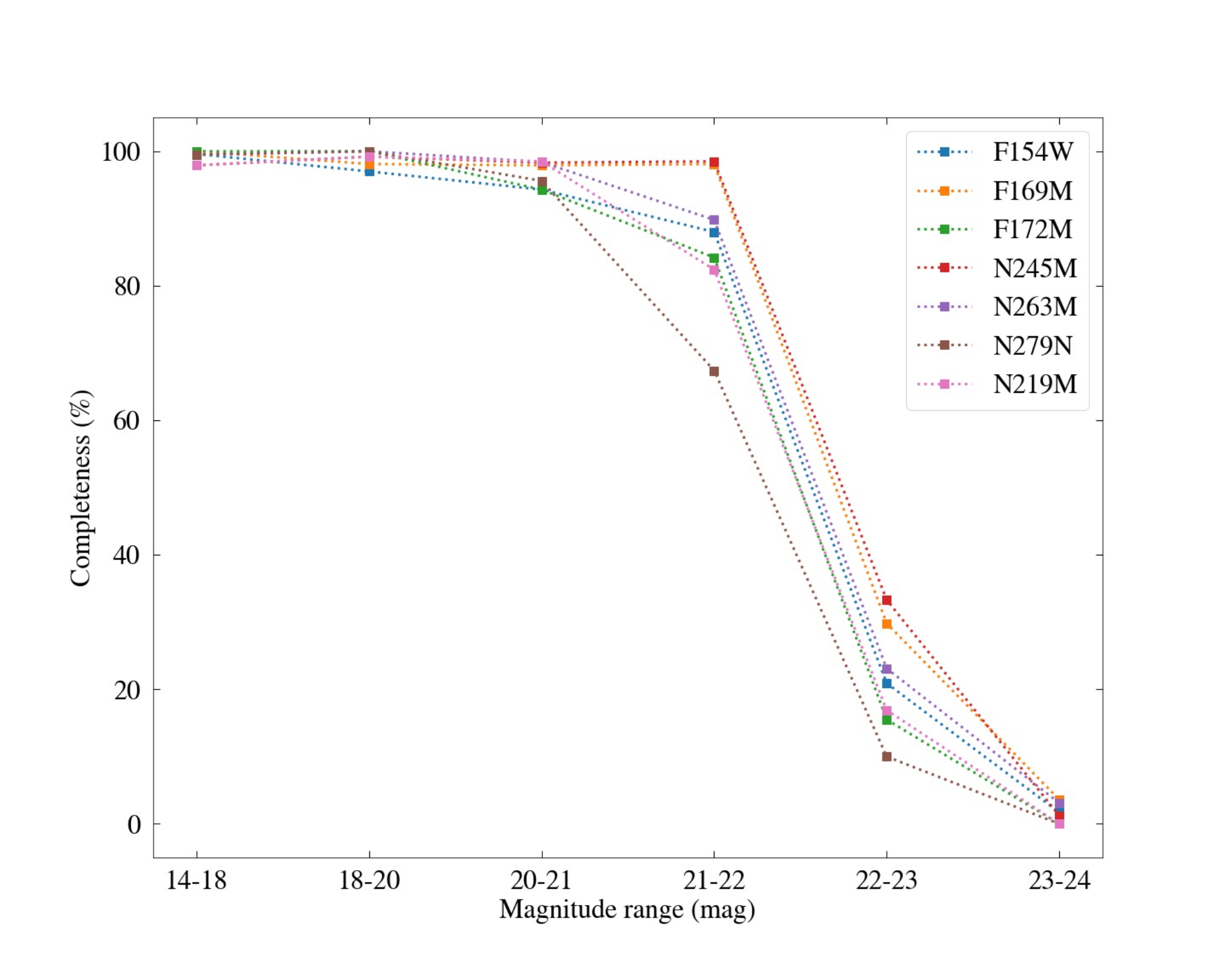
We also assessed the completeness of our photometry as a function of brightness by introducing artificial stars. We added artificial stars numbering about 10% of the point sources detected in each of the filters. They with pre-selected positions and brightness were added randomly (using the addstar routine in IRAF) to each of the filters, so as not to alter the crowding characteristics. After the addition of the artificial stars, the photometry of the frames were carried out in the usual procedure (see Section 3.1). The ratio of the number of recovered stars to that inserted gives a measure of the completeness of our photometry. The variation of the completeness factor as a function of brightness for different filters is given in Table 5 and shown in Fig. 7.
| Filter | No.of | gauss | moffat25 | moffat15 | lorentz | ||||
|---|---|---|---|---|---|---|---|---|---|
| stars | AC | Ratio | AC | Ratio | AC | Ratio | AC | Ratio | |
| F154W | 81 | -0.276 0.004 | 1.290 0.004 | -0.299 0.004 | 1.318 0.005 | -0.312 0.004 | 1.333 0.005 | -0.335 0.004 | 1.362 0.004 |
| F169M | 109 | -0.322 0.003 | 1.346 0.004 | -0.335 0.003 | 1.362 0.004 | -0.340 0.003 | 1.369 0.004 | -0.349 0.003 | 1.380 0.004 |
| F172M | 72 | -0.298 0.004 | 1.317 0.005 | -0.311 0.004 | 1.332 0.005 | -0.319 0.004 | 1.342 0.005 | -0.336 0.004 | 1.363 0.005 |
| N245M | 114 | -0.415 0.004 | 1.467 0.006 | -0.417 0.004 | 1.469 0.006 | -0.416 0.004 | 1.468 0.006 | -0.429 0.004 | 1.486 0.006 |
| N263M | 110 | -0.413 0.005 | 1.465 0.007 | -0.416 0.005 | 1.469 0.007 | -0.412 0.005 | 1.463 0.007 | -0.434 0.005 | 1.493 0.007 |
| N279N | 49 | -0.397 0.007 | 1.442 0.009 | -0.405 0.007 | 1.454 0.009 | -0.400 0.007 | 1.447 0.009 | -0.432 0.007 | 1.491 0.009 |
| N219M | 75 | -0.528 0.007 | 1.629 0.011 | -0.531 0.007 | 1.633 0.011 | -0.533 0.007 | 1.636 0.010 | -0.544 0.006 | 1.652 0.010 |
| Mag. range | F154W | F169M | F172M | N245M | N263M | N279N | N219M |
|---|---|---|---|---|---|---|---|
| 14-18 | 1.00 | 1.00 | 1.00 | 0.98 | 1.00 | 1.00 | 0.98 |
| 18-20 | 0.97 | 0.98 | 1.00 | 0.99 | 1.00 | 1.00 | 0.99 |
| 20-21 | 0.94 | 0.98 | 0.94 | 0.98 | 0.98 | 0.96 | 0.98 |
| 21-22 | 0.88 | 0.98 | 0.84 | 0.99 | 0.90 | 0.67 | 0.82 |
| 22-23 | 0.21 | 0.30 | 0.16 | 0.33 | 0.23 | 0.10 | 0.17 |
| 23-24 | 0.02 | 0.04 | 0.00 | 0.01 | 0.03 | 0.00 | 0.00 |
| S. No. | (deg) | (deg) | F154W | F169M | F172M | N245M | N263M | N279N | N219N | |||||||
|---|---|---|---|---|---|---|---|---|---|---|---|---|---|---|---|---|
| AB | Error | AB | Error | AB | Error | AB | Error | AB | Error | AB | Error | AB | Error | |||
| 1 | 17.483551 | -71.477719 | 19.274 | 0.049 | 19.206 | 0.047 | 19.194 | 0.059 | 19.127 | 0.033 | 19.034 | 0.036 | 18.999 | 0.065 | 18.992 | 0.059 |
| 2 | 17.501380 | -71.474138 | 19.861 | 0.064 | 19.638 | 0.057 | 19.817 | 0.079 | 19.870 | 0.047 | 19.655 | 0.049 | 19.612 | 0.086 | 19.354 | 0.070 |
| 3 | 17.411340 | -71.473069 | 21.085 | 0.112 | 21.079 | 0.111 | 20.556 | 0.111 | 20.625 | 0.066 | 20.402 | 0.068 | 20.453 | 0.127 | 20.244 | 0.106 |
| 4 | 17.516082 | -71.469507 | 16.307 | 0.012 | 16.281 | 0.012 | 16.355 | 0.016 | 16.361 | 0.009 | 16.322 | 0.010 | 16.377 | 0.019 | 16.217 | 0.017 |
| 5 | 17.426452 | -71.468917 | 20.073 | 0.070 | 20.053 | 0.069 | 19.800 | 0.078 | 19.392 | 0.037 | 19.257 | 0.040 | 19.223 | 0.072 | 19.383 | 0.071 |
| 6 | 17.546273 | -71.468802 | 20.399 | 0.082 | 20.105 | 0.071 | 20.354 | 0.101 | 20.214 | 0.055 | 20.149 | 0.061 | 20.020 | 0.104 | 20.007 | 0.095 |
| 7 | 17.442353 | -71.467313 | 20.776 | 0.097 | 20.816 | 0.098 | 20.722 | 0.119 | 20.704 | 0.068 | 20.415 | 0.069 | 20.343 | 0.121 | 20.348 | 0.111 |
| 8 | 17.218003 | -71.463924 | 21.673 | 0.147 | 21.519 | 0.135 | 21.242 | 0.152 | 20.926 | 0.076 | 20.469 | 0.071 | 19.995 | 0.103 | 20.581 | 0.123 |
| 9 | 17.332593 | -71.463868 | 19.558 | 0.055 | 19.511 | 0.054 | 19.564 | 0.070 | 19.589 | 0.041 | 19.494 | 0.045 | 19.235 | 0.072 | 19.401 | 0.072 |
| 10 | 17.548006 | -71.462470 | 19.460 | 0.053 | 19.380 | 0.051 | 19.239 | 0.060 | 19.085 | 0.032 | 18.945 | 0.035 | 18.877 | 0.061 | 19.004 | 0.060 |
| 11 | 17.657541 | -71.459780 | 21.125 | 0.114 | 21.621 | 0.142 | 21.294 | 0.155 | 21.068 | 0.081 | 20.820 | 0.083 | 20.774 | 0.147 | 20.699 | 0.130 |
| 12 | 17.542935 | -71.458877 | 21.101 | 0.113 | 21.374 | 0.127 | 20.951 | 0.133 | 20.993 | 0.078 | 20.598 | 0.075 | 20.195 | 0.113 | 20.533 | 0.121 |
| 13 | 17.443856 | -71.458562 | 21.740 | 0.151 | 21.481 | 0.133 | 21.444 | 0.166 | 21.265 | 0.088 | 21.284 | 0.103 | 20.749 | 0.145 | 20.726 | 0.132 |
| 14 | 17.666746 | -71.456551 | 20.290 | 0.078 | 20.238 | 0.075 | 20.164 | 0.092 | 20.040 | 0.050 | 19.816 | 0.052 | 19.720 | 0.091 | 19.847 | 0.088 |
| 15 | 17.537647 | -71.455490 | 20.427 | 0.083 | 20.316 | 0.078 | 20.184 | 0.093 | 20.267 | 0.056 | 19.953 | 0.056 | 19.913 | 0.099 | 20.157 | 0.102 |
Note. — The table in full is available in the electronic version of the article
IV Summary
In this work, we have analysed three pointings of SMC, observed by UVIT. From this analysis, we arrived at a catalogue of 11,241 UV sources in the three fields of SMC, and provide their AB magnitudes in a total of seven filters, three in FUV and four in NUV. The sample catalogue of 15 sources is given in Table 6. The full catalogue is available in the electronic version of the article. This catalogue will be of use to the astronomical community to address a large range of astronomical problems. We also carried out an evaluation of the relation between observed and saturation corrected UVIT magnitudes. We found that the observed UVIT magnitudes need to be corrected for the effects of saturation and PSF and provide empirical relations for the same.
Appendix A Saturation correction
In the NUV and FUV channels of UVIT, the occurrence of multiple photon events within 3 3 pixels () in a frame is detected as a single photon. Thus, for point sources with counts per frame 0.1, significant number of photons are not recorded. This effect of saturation needs to be taken into account while estimating the brightness of point sources from the measured count rates. Another possible source of saturation is the reduced multiplication of the photo electrons in the MCPs, reducing the final signal and hence reducing the probability of detection, when the local photon rate is high. However, this effect is estimated to be 5% for rates of 150 detected photons per second for a point source and has been ignored (Tandon et al. 2017). To correct for the effects of saturation, we adopted the empirical method outlined in Tandon et al. 2017. Essential steps in this method are: i) assuming Poisson statistics for the occurrence of multiple photons in a frame for 97% of the counts per frame in the full PSF (CPF5), an ideal correction (ICORR) was calculated (97% is arbitrarily chosen to discard counts in the outermost part of the PSF), ii) a relation (given in Equation A1) was derived relating the ideal correction to the actual correction found from detailed analysis of the frames, and iii) the actual correction was used to find the corrected counts per frame and hence the corrected counts per second as given in Equation A2.
| (A1) |
| (A2) |
Where 28.7 is the number of frames per second for the present observations. As we used the observed counts in a radius of 12 sub-pixels, the above process needs to be translated to obtain the corrected total counts per second from those observed in a radius of 12 sub-pixels. To do this, for various values of the corrected counts per second within the full PSF (CPS), the expected counts per second within a radius of 12 sub-pixels (CO12) were calculated as per the prescription in Equation A1, A2 and A3. We also assumed that all the saturation is limited to a radius of 12 sub-pixels. The values of CPS were fitted to a third order polynomial in CO12. This process is illustrated in the following equations:
| (A3) |
Here, is the correction factor to convert the counts per second in the full PSF (100 sub-pixels radius) to those in a radius of 12 sub-pixels in the absence of saturation, which is 0.893 for NUV and 0.886 for FUV (Tandon et al. 2020, see Table 11 of).
We define a saturation correction factor SAT as per Equation A4 and calculated SAT and CO12 for various values of CPS in the range 0.6 to 17. Next a polynomial fit was made relating SAT to CO12 as
| (A4) |
| (A5) |
References
- Agrawal (2006) Agrawal, P. C. 2006, Advances in Space Research, 38, 2989, doi: 10.1016/j.asr.2006.03.038
- Astropy Collaboration et al. (2013) Astropy Collaboration, Robitaille, T. P., Tollerud, E. J., et al. 2013, A&A, 558, A33, doi: 10.1051/0004-6361/201322068
- Bevington & Robinson (1992) Bevington, P. R., & Robinson, D. K. 1992, Data reduction and error analysis for the physical sciences
- Cohen et al. (2003) Cohen, M., Wheaton, W. A., & Megeath, S. T. 2003, AJ, 126, 1090, doi: 10.1086/376474
- Cornett et al. (1994) Cornett, R. H., Hill, J. K., Bohlin, R. C., et al. 1994, ApJ, 430, L117, doi: 10.1086/187452
- Cornett et al. (1997) Cornett, R. H., Greason, M. R., Hill, J. K., et al. 1997, AJ, 113, 1011, doi: 10.1086/118317
- de Grijs & Bono (2015) de Grijs, R., & Bono, G. 2015, AJ, 149, 179, doi: 10.1088/0004-6256/149/6/179
- Dufour (1984) Dufour, R. J. 1984, in IAU Symposium, Vol. 108, Structure and Evolution of the Magellanic Clouds, ed. S. van den Bergh & K. S. D. de Boer, 353–361, doi: 10.1017/S0074180900040481
- Gaia Collaboration et al. (2018) Gaia Collaboration, Mignard, F., Klioner, S. A., et al. 2018, A&A, 616, A14, doi: 10.1051/0004-6361/201832916
- Ghosh et al. (2021) Ghosh, S. K., Tandon, S. N., Joseph, P., et al. 2021, Journal of Astrophysics and Astronomy, 42, 29, doi: 10.1007/s12036-020-09686-z
- Ghosh et al. (2022) Ghosh, S. K., Tandon, S. N., Singh, S. K., et al. 2022, arXiv e-prints, arXiv:2203.07693. https://arxiv.org/abs/2203.07693
- Gordon et al. (2011) Gordon, K. D., Meixner, M., Meade, M. R., et al. 2011, AJ, 142, 102, doi: 10.1088/0004-6256/142/4/102
- Hagen et al. (2017) Hagen, L. M. Z., Siegel, M. H., Hoversten, E. A., et al. 2017, MNRAS, 466, 4540, doi: 10.1093/mnras/stw2954
- Harris et al. (2020) Harris, C. R., Millman, K. J., van der Walt, S. J., et al. 2020, Nature, 585, 357, doi: 10.1038/s41586-020-2649-2
- Hilditch et al. (2005) Hilditch, R. W., Howarth, I. D., & Harries, T. J. 2005, MNRAS, 357, 304, doi: 10.1111/j.1365-2966.2005.08653.x
- Hunter (2007) Hunter, J. D. 2007, Computing in Science & Engineering, 9, 90, doi: 10.1109/MCSE.2007.55
- Hutchings (1982) Hutchings, J. B. 1982, ApJ, 255, 70, doi: 10.1086/159804
- Lazzarini et al. (2019) Lazzarini, M., Williams, B. F., Hornschemeier, A. E., et al. 2019, ApJ, 884, 2, doi: 10.3847/1538-4357/ab3f32
- Leahy et al. (2020) Leahy, D. A., Postma, J., Chen, Y., & Buick, M. 2020, ApJS, 247, 47, doi: 10.3847/1538-4365/ab77a9
- Massey (2002) Massey, P. 2002, ApJS, 141, 81, doi: 10.1086/338286
- McKinney et al. (2010) McKinney, W., et al. 2010, in Proceedings of the 9th Python in Science Conference, Vol. 445, Austin, TX, 51–56
- Simons et al. (2014) Simons, R., Thilker, D., Bianchi, L., & Wyder, T. 2014, Advances in Space Research, 53, 939, doi: 10.1016/j.asr.2013.07.016
- Stetson (1987) Stetson, P. B. 1987, PASP, 99, 191, doi: 10.1086/131977
- Tandon et al. (2017) Tandon, S. N., Subramaniam, A., Girish, V., et al. 2017, AJ, 154, 128, doi: 10.3847/1538-3881/aa8451
- Tandon et al. (2020) Tandon, S. N., Postma, J., Joseph, P., et al. 2020, AJ, 159, 158, doi: 10.3847/1538-3881/ab72a3
- Tody (1986) Tody, D. 1986, in Society of Photo-Optical Instrumentation Engineers (SPIE) Conference Series, Vol. 627, Instrumentation in astronomy VI, ed. D. L. Crawford, 733, doi: 10.1117/12.968154
- Virtanen et al. (2020) Virtanen, P., Gommers, R., Oliphant, T. E., et al. 2020, Nature Methods, 17, 261, doi: 10.1038/s41592-019-0686-2
- Weingartner & Draine (2001) Weingartner, J. C., & Draine, B. T. 2001, ApJ, 548, 296, doi: 10.1086/318651