The IACOB projectPreprint: mbritavskiy@uliege.be
Abstract
Context. The empirical distribution of projected rotational velocities ( sin ) in massive O-type stars is characterised by a dominant slow velocity component and a tail of fast rotators. It has been proposed that binary interaction plays a dominant role in the formation of this tail.
Aims. We perform a complete and homogeneous search for empirical signatures of binarity in a sample of 54 fast-rotating stars with the aim of evaluating this hypothesis. This working sample has been extracted from a larger sample of 415 Galactic O-type stars that covers the full range of sin values.
Methods. We used new and archival multi-epoch spectra in order to detect spectroscopic binary systems. We complemented this information with Gaia proper motions and TESS photometric data to aid in the identification of runaway stars and eclipsing binaries, respectively. We also benefitted from additional published information to provide a more complete overview of the empirical properties of our working sample of fast-rotating O-type stars.
Results. The identified fraction of single-lined spectroscopic binary (SB1) systems and apparently single stars among the fast-rotating sample is 18% and 70%, respectively. The remaining 12% correspond to four secure double-line spectroscopic binaries (SB2) with at least one of the components having a sin ¿ 200 km s-1(8%), along with a small sample of 2 stars (4%) for which the SB2 classification is doubtful: these could actually be single stars with a remarkable line-profile variability. When comparing these percentages with those corresponding to the slow-rotating sample, we find that our sample of fast rotators is characterised by a slightly larger percentage of SB1 systems (18% vs. 13%) and a considerably smaller fraction of clearly detected SB2 systems (8% vs. 33%). Overall, there seems to be a clear deficit of spectroscopic binaries (SB1+SB2) among fast-rotating O-type stars (26% vs. 46%). On the contrary, the fraction of runaway stars is significantly higher in the fast-rotating domain (33-50%) than among those stars with sin ¡ 200 km s-1. Lastly, almost 65% of the apparently single fast-rotating stars are runaways. As a by-product, we discovered a new over-contact SB2 system (HD 165921) and two fast-rotating SB1 systems (HD 46485 and HD 152200) Also, we propose HD 94024 and HD 12323 (both SB1 systems with a sin ¡ 200 km s-1) as candidates for hosting a quiescent stellar-mass black hole.
Conclusions. Our empirical results seem to be in good agreement with the assumption that the tail of fast-rotating O-type stars (with sin ¿ 200 km s-1) is mostly populated by post-interaction binary products. In particular, we find that the final statistics of identified spectroscopic binaries and apparent single stars are in good agreement with newly computed predictions obtained with the binary population synthesis code BPASS and earlier estimations obtained in previous studies.
Key Words.
Stars: early-type – Stars: rotation – Stars: fundamental parameters – Stars: oscillations (including pulsations) – Techniques: spectroscopic1 Introduction
One decade ago, de Mink et al. 2013; de Mink et al. 2014 performed a detailed theoretical evaluation of the impact that binary interaction could have on the spin-rate properties of massive O-type stars (i.e. main sequence stars with masses in the range of 20 – 80 M⊙). This study was partly motivated by the necessity to provide an explanation for an empirical result already highlighted by Conti & Ebbets 1977; Wolff et al. 1982 and subsequently confirmed by some other authors (Simón-Díaz & Herrero 2014; Ramírez-Agudelo et al. 2013; Holgado et al. 2022, see further references in); namely: the spin-rate distribution of any investigated (large) sample of O-type stars (even in different metallicity environments) is characterised by a main component, including stars spinning with projected rotational velocities ( sin ) below 150 – 200 km s-1, and a tail of fast rotators reaching values of sin up to 400 – 600 km s-1. Such a tail of fast rotators normally comprises 20 – 25% of stars in the considered samples.
By performing a specific simulation of a massive binary-star population typical for our Galaxy and assuming continuous star formation, de Mink et al. 2014 found that binary interaction during main sequence evolution could easily explain the existence of the empirically detected tail of fast-rotating O-type stars. In brief, mass (and angular momentum) transfer from the initially more massive star (donor) to the lower mass companion (gainer) is an efficient mechanism to spin up the latter which, under certain circumstances, may become the more massive component of the binary system after Roche lobe overflow (Packet 1981; Pols et al. 1991, see also e.g.).
Indeed, by assuming the empirical distributions of mass ratios, orbital periods, and the corresponding binary fraction obtained by Sana et al. 2012 as input for their simulations, de Mink et al. 2013 ended up with a fraction of fast rotators (i.e. assuming they are characterised by having a sin 200 km s-1), which is very similar to the observed one. Furthermore, de Mink et al. 2013 provided some predictions regarding the expected type and percentage of binary products populating the tail of fast rotators in the sin distribution of O-type stars. This mainly includes mergers and mass gainers orbited by a hot stripped star or a compact degenerate object (neutron star or black hole).
In this context, we should also note that the merger scenario is considered as one of the mechanisms producing magnetic fields in massive stars (Ferrario et al. 2009; Schneider et al. 2016; Schneider et al. 2019, e.g.). In such magnetic massive stars, rotation is braked fast, so that mergers would lead to slow rotators. Since the debate remains open on the exact outcome of mergers, the merger scenario should still deserve particular attention when investigating the origin of fast rotators.
In addition, some of these fast-rotating O-type stars would be expected to be detected as runaway stars resulting from a disrupted binary after supernova explosion of the initially more massive component of the system (Blaauw 1961; Gies & Bolton 1986; Walborn et al. 2014, see e.g.). The latter would imply a complementary or alternative explanation to the dynamical ejection scenario from a stellar cluster to the occurrence of runaway events in the massive star domain (Portegies Zwart et al. 1999).
The empirical confirmation of these theoretical scenarios has important consequences for several topics of modern astrophysics, especially those influenced by our specific knowledge about massive star formation, evolution, and feedback. In these respects, it is important to recall that stellar rotation is known to play an important role in the evolution of high-mass stars (Maeder & Meynet 2000; Ekström et al. 2012, e.g.). It not only modifies the evolutionary paths followed by these stars, as well as their lifetimes and final fates, but it has also been proposed to induce the transport of core-processed elements to the stellar surfaces. There is clear evidence that a non-negligible percentage of massive O-type stars rotate at velocities fast enough to be affected by the aforementioned effects. Thus, we need to be careful while using the empirical information compiled for these fast-rotating O-type stars in order to constrain our theories of high-mass star formation and evolution. This is because the theories will be different if the stars have acquired their angular momentum during the star formation process or through any type of binary interaction. For example, if a large percentage O-type stars having a sin larger than 200 km s-1 are post-interaction binaries, proposed by de Mink et al. 2013; de Mink et al. 2014, using these stars to investigate the efficiency of rotational mixing in single star evolution models may lead to erroneous results and conclusions (Hunter et al. 2009; Cazorla et al. 2017b, e.g.).
Another point worth mentioning is the exotic nature of the possible companions to fast rotators. Indeed, short-period binary systems that are passing through the common-envelope phase may produce binary black holes or neutron star systems that can be progenitors of gravitational wave events (Langer et al. 2020, e.g.). These systems undergo a Roche-lobe overflow resulting in the donor becoming a Helium star while the accretor becomes a fast rotator of the OB-type. Taking into account subsequent evolution of such systems, BH/NS+OB configurations may arise. While some steps towards the detection of BH+OB systems have been taken (Villaseñor et al. 2021; Mahy et al. 2022; Banyard et al. 2022; Shenar et al. 2022a; Shenar et al. 2022b; Janssens et al. 2023, e.g.), our programme sample is one of the best compilations that can be used in the search of such systems. Finally, we may mention in this context that cooler fast-rotating stars showing Be-type signatures have shown hints of a post-interaction nature (Bodensteiner et al. 2020; Wang et al. 2021; Klement et al. 2022, e.g.).
As a continuation of the efforts devoted by the IACOB project (P.I. Simón-Díaz) to provide solid empirical foundations to our knowledge about the physical properties and evolution of massive OB-type stars (Simón-Díaz & Herrero 2014; Simón-Díaz et al. 2017; Holgado et al. 2020; Holgado et al. 2022, see e.g.), in this paper, we perform a complete and homogeneous search for empirical signatures of binarity in a statistically meaningful sample of several tens of fast-rotating Galactic O-type stars. Our ultimate goal is to evaluate the scenario proposed by de Mink et al. 2013; de Mink et al. 2014 to explain the existence of a tail of fast rotators in this stellar domain. To this aim, we use as starting point the results presented in Holgado et al. 2022, where we performed a reassessment of the empirical rotational properties of Galactic massive O-type stars using the results from a detailed analysis of ground-based multi-epoch optical spectra obtained in the framework of the IACOB & OWN surveys (see Sect. 2). The spectroscopic observations considered in Holgado et al. 2022 can now be complemented with an extended multi-epoch spectroscopic dataset (including a minimum of 3 – 5 epochs for all stars in the investigated sample of fast-rotators) and a set of superb quality data about proper motions and photometric variability recently delivered by the Gaia and TESS space missions.
The paper is organised as follows. In Sect. 2, we introduce the programme sample and the compiled observational data set. Sect. 3 describes the analysis we have performed (including a radial velocity analysis and Gaia and TESS data) and the literature overview regarding the programme sample. In Sect. 4, we discuss and interpret the obtained results. Sect. 5 presents the main conclusions of the paper.
2 Sample definition and observations
2.1 Programme sample
To build the sample that forms the basis for the study detailed in the present paper, we benefitted from information presented in Holgado et al. 2022. There, a detailed investigation of the spin-rate properties was performed for a sample of 285 Galactic O-type stars identified as apparently single or single-line spectroscopic binaries (SB1), using high-quality optical spectroscopic data gathered by the IACOB and OWN surveys (last described in Simón-Díaz et al. 2020 Simón-Díaz et al. 2020 and Barbá et al. 2017 Barbá et al. 2017, respectively).
Holgado et al. 2022 started from an initial sample of 415 Galactic O-type stars and excluded 113 double-line spectroscopic binaries, plus another 17 peculiar stars (i.e. presenting signatures in their spectra that are typically associated with Oe, Wolf-Rayet, or magnetic stars). For the remaining sample of 285 stars, they obtained estimates for the projected rotational velocities and other stellar parameters that can routinely be procured by means of a quantitative spectroscopic analysis. To this aim, they applied for each star the methodology described in Holgado et al. 2018 to the best S/N spectrum (Holgado et al. 2020, see also).
The estimated effective temperature (), the surface gravity (Herrero et al. 1992; Repolust et al. 2004, corrected from centrifugal forces, log gc, see), and sin allowed us to locate the sample in the spectroscopic HR diagram (Langer & Kudritzki 2014, sHRD,), as well as to build the corresponding global sin distribution. As indicated in Sect. 1, and illustrated by the right panel of Fig. 1 (Holgado et al. 2022, see also), this sin distribution is characterised by a dominant low velocity component and a tail of fast rotators extending up to 450 km s-1.
Following de Mink et al. 2013, this tail of fast rotators – especially above 200 km s-1– is expected to be mostly populated by the evolved post-interaction binaries. To empirically evaluate this hypothesis, we defined as our initial programme sample of stars those targets identified by Holgado et al. 2022 as having a sin 200 km s-1 (see Table 4). This corresponds to a total of 50 stars, distributed throughout the O-star domain in the sHR diagram as illustrated in the left panel of Fig. 1.
While this boundary in rotational velocity is somewhat arbitrary, as predicted by de Mink et al. 2013, it should allow us to minimise the presence of pre-interacting binary systems in the sample under study. Therefore, except for a small fraction of stars in the sin range between 200 and 300 km s-1(which could be short-period binary systems with individual components spun up by tides), the large majority of stars in our working sample should be (again in the context of de Mink’s scenario) mergers (i.e. genuinely single stars) or mass gainers in which the initially less massive star has now become an O-type star accompanied by a post-mass transfer object (i.e. a compact remnant or a stripped star) or a fast-rotating runaway star. We also note that while we have assumed the same boundary in equatorial velocity () as in de Mink et al. 2013, we are actually using the quantity sin and not to build our working sample of fast rotators. Therefore, there could still be fast-rotating stars in Holgado’s sample that we are missing because their rotational axis has a low inclination angle. This effect will be taken into account in the discussion and interpretation of our results (see e.g. Fig. 7 and Sects. 4.2 and 4.6).
For the sake of completeness, while we were not able to obtain accurate individual sin measurements for the two components of those stars identified as double-line spectroscopic binaries (SB2), we carried out a careful inspection of all available spectra for the 113 SB2 systems in the initial sample to identify those in which at least one of the components could have a sin larger than 200 km s-1. This information allowed us to have an estimate of the percentage of such systems with at least one of the two components being a fast rotator (see Sect. 4.4 and Table 2). The four identified systems fulfilling this criterion are quoted at the bottom of Table 4.
2.2 Multi-epoch spectroscopic observations
As was the case of previous papers of the IACOB series dealing with O-type stars (Holgado et al. 2018; Holgado et al. 2020; Holgado et al. 2022, see e.g.), the bulk of the spectroscopic observations used in this work comes from three high-resolution spectrographs: the FIES instrument (Telting et al. 2014, resolving power, R46 000 or 25 000,) attached to the 2.56-m Nordic Optical Telescope (NOT), the HERMES spectrograph (Raskin et al. 2011, R85 000,) attached to the 1.2-m Mercator telescope, and the FEROS spectrograph (Kaufer et al. 1997, R48 000,) presently installed at the MPG/ESO2.2-m telescope. The former two instruments are both located in the Roque de los Muchachos observatory (La Palma, Spain), while the latter has been operating in La Silla observatory (Chile) since 2002. Detailed information on the collected spectroscopic data set can be found in Table 1 of Holgado et al. 2018.
Our programme sample comprises Galactic O-type stars in both hemispheres covering a range in B magnitude from 2.5 and down to 11 mag. Those stars observable from the Canary Island observatory were observed as part of the IACOB survey (P.I. Simón-Díaz) during several observing runs allocated between 2008 and 2016. This survey initially included a minimum of three epochs per star; however, we also devoted several new additional campaigns since 2017 (P.I. Holgado) to increase the number of available epochs for the subsample of 23 fast rotators visible from the Canary Islands’ observatory. These extra observations, which have allowed us to cover a time-span of more than ten years with more intense time coverage between 2017 and 2018, do not only include FIES and HERMES spectra, but also up to ten additional epochs obtained with the SES high-resolution spectrograph (Strassmeier et al. 2004) attached to the STELLA1.2-m robotic telescope operating at Izaña observatory (Tenerife, Spain).
For those stars observable from La Silla, the multi-epoch spectroscopic dataset compiled for this work was mostly obtained in the framework of the OWN spectroscopic survey11 1 We note there are seven stars observable from both the La Silla and the Canary Islands observatories. (P.I. Barbá) between 2007 and 2017. In addition, these observations were complemented with a few spectra downloaded from the ESO-FEROS archive22 2 http://archive.eso.org/wdb/wdb/adp/phase3_spectral/form.
The full list of 54 fast-rotating stars comprising our programme sample33 3 This includes the four detected SB2 stars with at least one of the components having a sin larger than 200 km s-1. is quoted in Table 4, where we also indicate the corresponding spectral classifications (Maíz Apellániz et al. 2013, as provided in version 4.1 of the Galactic O-star catalog, GOSC,), the number of FIES, HERMES, FEROS, and STELLA spectra initially available, and the total time-span covered by each set of multi-epoch spectra. Generally speaking, after discarding those spectra with low (less than 5) in the 5875 Å region, we have been able to compile a minimum of 4 epochs for almost 90% of the stars in the sample (see column 8 of Table 4), reaching up to 10 epochs in more than 50% of them. In addition, for some bright Northern targets, we could gather more than 25 epochs. Regarding the covered time-span, except for a few cases, we were able to reach a minimum of 3 years and up to 10 – 15 years for 20 stars (see last column of Table 4).
Thanks to Gaia-EDR3, we also have information about parallaxes for all stars in our working sample (see also Sect. 2.3). By taking as a first approach the median of the geometric distances provided in Bailer-Jones et al. 2021, we see that 51 of the 54 stars are closer than 3 kpc, and only 6 of them have a RUWE value44 4 We recall that this quantity (the renormalised unit weight error, RUWE) can be used as a quality flag of the Gaia astrometric solution for each individual target. Following recommendations by the Gaia team, information for those stars with a RUWE value above 1.4 must be handle with care. larger than 1.4 (see Table 5).
As described in Sect. 3.1.1, having access to this information allowed us to obtain estimates for other stellar parameters (radii, luminosities) beyond what can be obtained by spectroscopic means, namely, projected rotational velocities, effective temperatures, surface gravities, or surface abundances of certain elements.
2.3 Other sources of empirical data considered in this work
In addition to our main multi-epoch spectroscopic observations described in previous section, we also benefitted from various other sources of empirical data including (a) photometric variability as provided by the light curves obtained by the TESS mission (Ricker et al. 2015), (b) the proper motions delivered by the Gaia mission (Gaia Collaboration et al. 2021), and (c) information about possible close-by visual companions as provided by the Gaia mission, as well as other on-ground high spatial resolution surveys such as the AstraLux optical survey (Maíz Apellániz 2010), the Southern Massive Stars at High angular resolution survey (Sana et al. 2014, SMASH,), and the Fine Guidance Sensor resolution survey (Aldoretta et al. 2015, FGS,).
Lastly, we also searched for additional info in the literature about whether any of the programme sample of fast-rotating stars had been previously identified as a spectroscopic, eclipsing, and/or X-ray binary. In this regard, we paid special attention to some specific studies providing information about the orbital parameters of previously detected binaries (see Sect. 3.2).
3 Gathering empirical information
Table 1 summarises all the empirical information of interest compiled for this paper regarding our programme sample (excluding the four clearly detected SB2 systems), ordered by increasing rotational velocity. In addition to the spectral classification (column 2), we quote the projected rotational velocity (column 3), the peak-to-peak amplitude of radial velocity variability, as measured from all available spectra per star (column 4), and the assigned spectroscopic binarity status after a first visual inspection of the variability of the He i 5875 line-profile (column 6).
The above-mentioned information – mainly obtained from the spectroscopic data set – is also complemented with other information resulting from the analysis of the additional empirical data mentioned in Sect. 2.3. The latter includes the type of variability detected in the TESS light curves (column 7), a determination of whether some close-by visual companions have been detected within 1 and 2 arcmin, respectively (column 9), the runaway status resulting from the analysis of the proper motions provided by Gaia and other studies in the literature (column 10) and, lastly, the final binary status established for each individual target after revisiting the literature and a more detailed analysis of the available radial velocity curves (column 11).
We list the physical parameters of our sample, gathered from Holgado 2019 and associated papers, in Table 5. We include estimates for the effective temperature (, column 2), the parameter (defined as 4/, see Langer & Kudritzki 2014, column 3, where is the surface gravity corrected from centrifugal forces), as well as the stellar luminosity and radius (columns 4 and 5, respectively), based on the individual Gaia-EDR3 distances (column 9) provided by Bailer-Jones et al. 2021. Below, we describe how each of these pieces of empirical information was obtained.
| Name | SpC | sin | RVPP | SB tag | Phot. var. | X-ray | Contamination | Runaway? | Final binary | |
|---|---|---|---|---|---|---|---|---|---|---|
| [km s-1] | [km s-1] | [km s-1] | (TESS) | (1′ and 1′-2′) | (Gaia+lit.) | status | ||||
| BD+36∘4145 | O8.5 V(n) | 200 3 | 3.5 1.1 | 1.2 | LPV | SLF | 0+0 | no | LS | |
| HD 216532 | O8.5 V(n) | 200 3 | 15.0 3.8 | 3.8 | LPV | PQ (+fr¿5) | 0+1 | no | LS | |
| HD 163892 | O9.5 IV(n) | 201 12 | 83.50 9.1 | 26.3 | SB1 | 0+0 | no | SB1 () | ||
| HD 210839 | O6.5 I(n)fp | 201 8 | 28.5 5.5 | 6.3 | LPV/SB1? | SLF | a | 0+0 | yes | LS (*) |
| HD 308813 | O9.7 IV(n) | 205 5 | 41.5 6.7 | 15.4 | SB1 | ? | l | 0+1 | no | SB1 |
| HD 36879 | O7 V(n)((f)) | 205 6 | 10.0 2.5 | 3.2 | LPV | SLF | 0+0 | yes | LS | |
| HD 37737 | O9.5 II-III(n) | 209 11 | 156.5 9.9 | 48.3 | SB1 | EB | no | SB1 | ||
| HD 152200 | O9.7 IV(n) | 210 32 | 32.0 6.5 | 12.8 | SB1 | RM | b | 0+1 | no | SB1 |
| HD 97434 | O7.5 III(n)((f)) | 215 22 | 14.5 3.5 | 6.1 | LPV | SLF | b | 0+2 | no | LS |
| HD 24912 | O7.5 III(n)((f)) | 224 8 | 29.0 4.7 | 6.2 | LPV/SB2? | c | 0+0 | yes | LS (*) | |
| BD+60∘2522 | O6.5 (n)fp | 231 23 | 24.5 5.8 | 8.4 | LPV/SB2? | SPB | k | 0+0 | yes | LS (*) |
| HD 89137 | ON9.7 II(n) | 233 3 | 3.0 1.3 | 1.3 | LPV | SLF (+fr¿5) | yes | LS | ||
| BD+60∘134 | O5.5 V(n)((f)) | 234 9 (*) | 7.5 3.4 | 3.0 | LPV | SLF | yes | LS | ||
| HD 172175 | O6.5 I(n)fp | 243 20 | 19.5 7.7 | 9.7 | LPV | yes | LS | |||
| HD 165246 | O8 V(n) | 254 8 | 126.0 14.9 | 36.3 | SB1 | EB | 1+0 | no | SB1 | |
| HD 5689 | O7 Vn((f)) | 256 40 | 12.0 3.4 | 4.2 | LPV | SLF | 0+0 | yes | LS | |
| HD 124314 | O6 IV(n)((f)) | 256 10 | 33.0 10.2 | 9.9 | LPV/SB2? | SLF | 2+0 | no | LPV/SB2? | |
| HD 192281 | O4.5 IV(n)(f) | 261 5 (*) | 19.5 8.6 | 5.6 | LPV | SLF + rot? | 0+0 | yes | LS | |
| HD 76556 | O6 IV(n)((f))p | 264 11 | 10.5 7.3 | 4.4 | LPV | SLF + rot? | i | 1+1 | no | LS |
| HD 41997 | O7.5 Vn((f)) | 272 12 | 23.5 4.8 | 6.0 | LPV | SLF | 0+0 | yes | LS | |
| HD 124979 | O7.5 IV(n)((f)) | 273 6 | 12.0 3.3 | 3.8 | LPV | SLF | yes | LS | ||
| HD 155913 | O4.5 Vn((f)) | 282 10 (*) | 8.5 8.0 | 3.1 | LPV | SLF + rot? | 0+0 | yes | LS | |
| HD 175876 | O6.5 III(n)(f) | 282 16 | 35.5 6.9 | 10.2 | LPV/SB2? | 0+0 | yes | LS (*) | ||
| HD 15137 | O9.5 II-IIIn | 283 7 | 44.0 6.3 | 10.8 | LPV/SB1? | SLF | 0+0 | yes | SB1 (*) | |
| HD 28446A | O9.7 IIn | 291 10 | 29.0 7.5 | 7.0 | LPV | SLF (+fr¿5) | 1+0 | no | LS | |
| HD 15642 | O9.5 II-IIIn(*) | 293 10 | 23.5 6.6 | 7.6 | LPV | SLF | 0+1 | yes | LS | |
| HD 90087 | O9.2 III(n) | 295 2 | 11.5 3.4 | 4.3 | LPV | no | LS | |||
| HD 165174 | O9.7 IIn | 299 11 | 59.5 7.4 | 18.3 | SB1 | d | 0+0 | no | SB1 | |
| HD 52266 | O9.5 IIIn | 299 7 | 35.0 6.0 | 10.1 | LPV | SLF | 0+0 | no | LPV/SB1? (*) | |
| HD 91651 | ON9.5 IIIn | 304 16 | 21.5 5.8 | 6.2 | LPV/SB2? | Cep | 0+0 | no | LPV/SB2? | |
| HD 228841 | O6.5 Vn((f)) | 311 8 (*) | 18.0 7.3 | 5.5 | LPV | SLF | i | yes | LS | |
| HD 52533 | O8.5 IVn(*) | 312 14 | 166.0 27.7 | 54.4 | SB1 | EB | 3+0 | no | SB1 () | |
| BD+60∘513 | O7 Vn | 313 11 (*) | 27.5 7.4 | 12.2 | LPV | SLF + rot? | e | 1+0 | no | LS |
| HD 229232 | O4 Vn((f)) | 313 11 (*) | 36.0 17.7 | 13.4 | LPV | SLF + rot? | 1+0 | yes | LS | |
| HD 13268 | ON8.5 IIIn | 316 10 | 21.0 5.4 | 5.2 | LPV | 0+0 | yes | LS | ||
| HD 14442 | O5 n(f)p | 320 14 (*) | 15.0 10.7 | 7.0 | LPV | SPB? | 0+1 | no | LS | |
| HD 41161 | O8 Vn | 322 8 | 10.5 3.8 | 3.0 | LPV | SLF | 0+0 | yes | LS | |
| HD 149452 | O9 IVn | 323 14 | 1.5 1.2 | 0.8 | LPV | SLF | 1+0 | yes | LS | |
| HD 203064 | O7.5 IIIn((f)) | 323 8 | 42.0 8.7 | 10.6 | LPV/SB1? | SLF | 0+0 | yes | LS (*) | |
| HD 326331 | O8 IVn((f)) | 323 7 | 17.5 5.2 | 4.4 | LPV | SLF | f | 2+2 | no | LS |
| HD 46485 | O7 V((f))nvar? | 334 16 | 29.5 13.6 | 9.1 | LPV | EB+RM | 0+0 | no | SB1 (*) | |
| HD 46056A | O8 Vn | 365 26 (*) | 29.0 11.6 | 8.6 | LPV | PQ (+fr¿5) | 1+0 | no | LS | |
| HD 117490 | ON9.5 IIInn | 369 10 | 17.0 6.6 | 4.8 | LPV | SLF (+fr¿5) | 0+2 | yes | LS | |
| HD 102415 | ON9 IV:nn | 376 4 | 35.0 10.8 | 12.0 | LPV | SLF (+fr¿5) | 0+1 | no | LS | |
| HD 93521 | O9.5 IIInn | 379 14 (*) | 48.5 8.0 | 11.2 | LPV | SLF (+fr¿5) | …g | 0+0 | yes | LS |
| HD 217086 | O7 Vnn((f))z | 394 9 | 15.5 8.3 | 4.9 | LPV | SLF | j | 0+0 | no | LS |
| HD 14434 | O5.5 IVnn(f)p | 395 12 (*) | 21.0 11.1 | 8.5 | LPV | SLF | h | 0+0 | yes | LS |
| HD 191423 | ON9 II-IIInn(*) | 397 18 | 37.5 9.6 | 9.6 | LPV | SLF | 0+0 | yes | LS | |
| HD 149757 | O9.2 IVnn | 400 8 | 32.0 9.5 | 4.7 | LPV | c | 0+0 | yes | LS | |
| ALS 12370 | O6. 5Vnn((f)) | 444 13 (*) | 15.0 11.8 | 5.6 | LPV | SLF + rot/EV? | no | LS |
In this table we list the measurements of peak-to-peak amplitude of variation (RVPP) and standard deviation () of all radial velocity measurements for each star. Apart from this, we indicate the spectroscopic binary and runaway status (’SB tag’ and ’runaway?’ columns, respectively), the type of detected photometric variability (’phot. var.’ column), the relative X-ray flux (’X-ray’ column), and the number of detected visual companions within 1 arcmin and between 1 and 2 arcmin, respectively (’contamination’ column). In the column ’final binary status’ we indicate our final decision regarding spectroscopic binary status. Eclipsing and spectroscopic binaries in the sample, as well as those stars identified to show ellipsoidal variability in the TESS light curves are highlighted in bold.
sin : In those stars marked with (*) the use of the He ii 5411 line was necessary to estimate the sin ;
SB tag: LPV – line profile variable; SB1, SB2 – one or two spectroscopic binary respectively; LPV/SB1?, LPV/SB2? – uncertain spectroscopic binaries;
Phot. var.: SPB/ Cep – coherent low/high frequency variability, respectively; SLF – stochastic low frequency variability; EB – eclipsing binary; EV – ellipsoidal variable; rot? – possible rotational modulation; RM – reflection modulation; PQ – poor quality of the TESS light curve; fr5 – existence of prominent peaks at frequencies larger than 5 d-1; – no TESS data or no data regarding visual components; ”?” – unknown periodic photometric modulation.
X-ray: a – Rauw et al. 2015, – Nazé 2009; Bhatt et al. 2010, d – Nazé et al. 2020, e – Rauw & Nazé 2016, f – Sana et al. 2006; Nazé 2009, g – Rauw et al. 2012, h – Nazé 2009, c – Nazé & Motch 2018; Cohen et al. 2021, i – this work, j
– Getman et al. 2006, k – Toalá et al. 2020, l – Nazé et al. 2013.
Final binary status: LS – likely/apparently single star. Those stars marked with a (*) symbol have changed their SB status (compared to column 5) after taking into account all available empirical information (see Sect 3.3.1 for details). In addition, although we keep them as SB1 for the purposes of this paper, Mahy et al. 2022 have identified faint lines of a secondary component using a disentangling technique in a much larger spectroscopic data set in those stars marked with a ().
3.1 Empirical information extracted from the spectra
3.1.1 Spectroscopic and fundamental parameters
Throughout this paper, we consistently use the same set of spectroscopic parameters (basically and log ) determined by Holgado et al. 2020 and later utilised by Holgado et al. 2022. The corresponding estimates and associated uncertainties are indicated in columns 2 and 3 of Table 5. As commented in Sect. 2.1, these data allow us to locate our programme sample of stars in the sHRD (see red dots in the left panel of Fig. 1)
In addition, the above-mentioned (spectroscopic) parameters were also complemented with other fundamental parameters, such as the radii, luminosities, and spectroscopic masses, which could be derived by considering the extinction corrected V magnitudes provided by Maíz Apellániz & Barbá 2018 and the Gaia-EDR3 distances quoted in Bailer-Jones et al. 2021. All these additional information can be found in Table 5.
3.1.2 Projected rotational velocities
Regarding the projected rotational velocities ( sin ), instead of directly using the values obtained by Holgado et al. 2022, we decided to repeat the line-broadening analysis but this time using all available FIES, HERMES, and FEROS spectra per star. This way we wanted to investigate what is the associated uncertainty in the derived sin resulting from any potential source of spectroscopic variability affecting the line profiles. In addition, those cases in which an important scatter in the time-dependent sin measurements is present could also be an indication that the star is actually a double-line spectroscopic binary.
To this aim, we applied again the iacob-broad tool (Simón-Díaz & Herrero 2014) to the same diagnostic line considered in Holgado et al. 2022. As commented in that paper, for the sake of homogeneity, we tried to use the O iiii 5591 line in all cases. However, it was only possible for 40% of the stars of the sample. For the rest of the stars, in which the O iii line appear too weak and shallow due to the high sin , we needed to use either the He i 5015 line (37%) or the He ii 5411 line (23%).
The results of this multi-epoch analysis are presented in column 3 of Table 1, where we indicate the mean values and associated standard deviations computed from the goodness-of-fit solutions provided by iacob-broad. These new estimates are then compared with those obtained by Holgado et al. 2022 in Fig. 2. Generally speaking, there is a very good agreement between both determinations and, except for a few (6) stars, the standard deviation resulting from the multi-epoch analysis is not larger than 5 – 6%.
In fact, the obtained standard deviation of the sin measurements is better than 10% in all stars but three (HD 152200, BD+60∘2522, and HD 5689), where it ranges between 15 and 20%. Interestingly, the TESS light curve of HD 152200 shows reflection modulation variability (see Sect.3.3.1), likely produced by a deformation of the star, hence affecting the sin measurements depending on the considered orbital phase. From visual inspection of the variability of some of the line-profiles of BD+60∘2522, we were not completely sure at first whether this star was a two-component spectroscopic binary (see Sect. 3.1.4), something which could explain the measured scatter in the sin estimates. Regarding HD 5689, we did not notice any peculiarities; however, we suggest using high deviation in sin as a hint for the possible identification of a faint companion or of peculiar photometric variability.

3.1.3 Radial velocities
Deriving radial velocities () in stars with broad line profiles is a challenging task. Significant spectral broadening caused by fast stellar rotation affects the shape of the spectral line and simple Gaussian-Lorentzian fitting of such line profiles is not efficient. In addition, other effects such as line blending, the fact that rotational broadening makes the lines to become much shallower, or the occurrence of line profile variability within the broad line-profiles, hinder the application of such fitting technique. In this case, the use of a cross-correlation technique – being aware that it has some limitations as well, especially when applied to spectra with a limited signal-to-noise ratio – becomes a viable solution. While this technique allows the possibility to consider a spectral window including several lines, its application to a well isolated line is also a valid option.
For this work, we use the cross-correlation technique described in Zucker 2003. We refer the reader to that paper for a detailed description of how a estimate and its associated uncertainty can be obtained from the cross-correlation function (CCF) resulting from a specific observed spectrum and an adequate reference spectrum.
In particular, we decided to apply this technique to just one prominent and unblended diagnostic line which is present in all stars of our programme sample: He i 5875. This decision was taken after evaluating the possibility of using a larger set of diagnostic lines present in the optical spectra of O-type stars (6 in total). As illustrated in Fig. 11, the main outcome of this exercise was that the attempt of using other lines beyond He i 5875 was neither improving the accuracy in the estimations (see below for definition of this quantity) or importantly modifying the results obtained using just the most prominent (and always present) He i line.
Lastly, we are aware that also He i 5876 line can be affected by stellar wind in some specific cases, this effect should not significantly affect the shape of the CCF if the wind emission is not very pronounced as expected for our sample, which is mostly composed of late O-type stars. Indeed, one of the advantages of the cross-correlation approach is that the behavior of the CCF does not depend on the relative distribution of the input data, that is, if we cross-correlate spectral lines with different widths, it does not affect the resulting function. This is why we can securely cross-correlate one convoluted line profile template with the rest of the spectra even if the lines change width or shape.
Technically speaking, we started by fitting a rotationally convolved (synthetic) profile to the He i 5875 line of the first spectrum in the multi-epoch data set available for a given star (see e.g. the top panel in Fig. 3). Then, by taking this synthetic line profile as our reference, we cross-correlated the rest of available spectra in the same wavelength range, thus obtaining a CCF as depicted in bottom panel of Fig. 3.


As a result, we obtained measurements relative to the first spectrum and their associated uncertainties for all available spectra. Based on these values, we calculated the peak-to-peak amplitude of radial velocity variability () following the various steps described below55 5 Tables xx and xx with individual measurements for each star and estimates are only available in electronic form at the CDS via anonymous ftp to cdsarc.cds.unistra.fr (130.79.128.5) or via https://cdsarc.cds.unistra.fr/cgi-bin/qcat?J/A+A/.
First, to make sure that only reliable measurements are considered, we calculate the S/N of our diagnostic line for each spectrum in the time-series. This quantity is defined as:
| (1) |
where min is the flux at the core of the line-profile and is the standard deviation of the normalised flux between 5855 and 5865 Å, a spectral window which only includes continuum points. Basically, this quantity indicates how prominent the spectral line is with respect to the continuum noise.
After evaluating several options, we decided to exclude all RV estimates for spectra with a 5. Even with this conservative threshold, most of the initially available spectra endure to the end of this cleaning process, indicating the good quality of our spectroscopic data set. The estimates of and overall for all measured spectra as a function of uncertainty in are presented in Fig. 13.
Then, in order to compute a final estimate of , we use the pair of measurements that maximises the quantity:
| (2) |
defined in Sana et al. 2013, where and refer to two different spectra from the time-series of a given star, and and are the individual uncertainties of the radial velocity measurements and , respectively. This approach helps to identify from the most accurate measurements by taking into account the individual uncertainties of radial velocity measurements. Also, the uncertainty associated with the final estimate of is computed as () = .
3.1.4 Visual inspection of line-profile variability
Orbital motion is not the only effect that can led to the detection of large radial velocity variations in O-type stars, especially in the case of fast rotators. As shown elsewhere (Fullerton et al. 1996; Aerts et al. 2014; Simón-Díaz et al. 2017, e.g.), the line profiles of most O- and B-type stars are often subject to various types of variability due to, for instance, stellar pulsations or spots. In addition, in the case of the He i 5875 line a non-spherically symmetric wind could also produce some variability which could be erroneously interpreted as empirical evidence of the star being a spectroscopic binary (SB) if only the measurements are taken into account.
We illustrate this argument in Fig. 4, where we show the detected line-profile variability in six illustrative examples including two unambiguously identified SB1 systems among our working sample, plus another four cases in which, despite a relatively high having been measured (reaching up to 48.5 km s-1 in one of the cases66 6 HD 93521, an O9.5 IInn star which has been extensively studied in the literature (e.g. Howarth & Reid 1993; Rauw et al. 2012; Gies et al. 2022, and references therein), but never identified as spectroscopic binary.), the detected variation in is likely produced by intrinsic line-profile variability.
Taking into account these ideas, we decided to complement the information about the measured with the outcome from a visual inspection of the detected variability of the He i 5875 line profile in all stars in our programme sample, classifying each star as being part of one of the following subgroups: ’LPV’, that is, line profile variables ’SB1’, ’LPV/SB1?’, and ’LPV/SB2?’. This information is provided in ’SB tag’ column of Table 1.
We used the LPV tag to identify stars which are likely single (LS) as we only detected small variations in the shape of the He i 5875 line-profiles. In an opposite situation, if a significant shift of the entire spectral line is detected visually, we classified the star as SB1. If the detected line-profile variability is not prominent, but there seems to be an overall shift of the line, we consider the star as an unclear SB1 and marked it as ’LPV/SB1?’.
In addition to this, we identified five SB2 candidates for which we were not completely sure about their spectroscopic binary nature. Hence, these stars were provisionally labeled as ’LPV/SB2?’. One interesting example of this type is HD 24912 ( Persei). In this case, the line-profile variability is most probably a consequence of the existence of co-rotating bright spots on the surface of the star, as detected by Ramiaramanantsoa et al. 2014, using photometric observations provided by the MOST satellite, and, hence, it is not an SB2 system. We excluded this star from the final statistics of ’LPV/SB2?’. Further notes on the other four targets can be found in Appendix B, along with a final decision of their revised spectroscopic binary status.
When presenting the final statistics of detected spectroscopic binaries (Sect. 4.4 and Table 2) among our sample, the ’surviving’ SB2 candidates will be added to the other four clearly detected SB2 systems77 7 Indeed, one of them is detected as a SB3 system, see Appendix B. included in the initial sample of 415 O-type stars for which we have found that at least one of the two components has a sin larger than 200 km s-1. For reference purposes, we also show two illustrative examples of the detected line-profile variability in the case of these double-line spectroscopic binary systems (see Fig. 4).
In this regard, we also provide here some further comments about the strategy we followed to identify SB2 systems. Again, our main diagnostic line for visual detection of double line spectroscopic binaries has been the He i 5875 line. This is not only one of the stronger lines in the spectra of O-type stars, but is also a line which remains strong in the full B star domain. This characteristic makes the line perfect to detect any secondary component hidden in the spectrum, even in cases where the sin of this second component is large and, hence, the line is greatly diluted. As a consequence, we can state with a high degree of confidence that given the quality of our spectroscopic data set (in terms of resolving power and S/N), this first visual inspection allows us to detect all possible companions contributing down to 10 – 20 % of the total flux of the system in the optical range, especially when we have enough epochs and the amplitude of of this (fainter) secondary component is larger than 70 – 80% of the sin of the primary.
Obviously, there will be certain cases in which this visual inspection will fail, specifically when the amplitude of variability of the fainter companion is less than 50% of the sin of the more luminous star. This case is expected to affect more importantly to stars with larger sin (i.e. the fast-rotator domain), thus leading to situations as those described above, where we are not sure if the detected line profile variability is due to any type of intrinsic variability in a single star or the presence of a companion (the LPV/SB2? case). To minimise the number of such cases, we specifically increase the number of available epochs in the sample of fast rotators and also explored more carefully other diagnostics lines which could help us to decide if we have a SB2 system or a LPV case. Also, we explored the possible detection of eclipses in the available TESS light curves (see Sect. 3.2.2), as well as the potential identification of close-by companions using high angular-resolution images (see Sect. 3.3.2) in order to complement the spectroscopic information with the aim of minimizing as much as possible the effect of observational biases in our detection of both single- and double-line spectroscopic binary systems.
Some additional notes about how the above-mentioned possible observational biases could be affecting the resulting statistics of detected spectroscopic binaries in stars in both the faster and slower rotating samples can be found in Sect. 4.4.
3.2 Empirical information extracted from Gaia and TESS data
The and TESS missions have provided a unique opportunity to have access to very valuable information of interest for our study in a homogeneous (and almost unbiased) way.
On the one hand, the proper motions delivered by -EDR3 (Gaia Collaboration et al. 2021) can be used to identify runaway stars. Some of these runaways are expected to be produced by the dynamical ejection of the surviving companion in a high-mass binary system after a supernova explosion event. Following de Mink et al. 2013, an important fraction of the O-type stars with sin 200 km s-1 are the mass gainers in binary systems after Roche-lobe overflow of the initially more massive star. In this sense, it is interesting to know, not only which of the stars in our programme sample are identified as a runaway star, but also to compare the percentage of runaways detected in the slow- and fast-rotator samples of O-type stars investigated in Holgado et al. 2022.
On the other hand, the high quality light curves provided by the TESS mission for almost all our programme stars (with the caveats described in Sect. 3.2.2), allow us to search for signatures of hidden companions not detected through our multi-epoch spectroscopy. Also, although such study is out of the scope of this paper, a thorough investigation of the detected photometric variability (by means of standard asteroseismic data analysis techniques) can provide new insights about the evolutionary nature of fast rotators.
3.2.1 Detection of runaway star candidates among Galactic O-type stars using Gaia ED3 proper motions
It has been known since the 1950s that some OB stars move at high speeds through the Galaxy as a consequence of dynamical interactions between three or more bodies in stellar clusters or of supernova explosions in binary systems (Zwicky 1957; Blaauw 1961; Poveda et al. 1967). Some of the stars are ejected with velocities higher than 30 km s-1. Those are called runaway stars (Hoogerwerf et al. 2001) and can be easily found with Gaia astrometry (Maíz Apellániz et al. 2018). The slightly slower ones defined as walkaway stars are more common but more difficult to identify (Renzo et al. 2019).
In order to identify runaway stars one needs to calculate their 3D velocity with respect to their local standard of rest (LSR). Strictly speaking, one should differentiate between the ejection velocity and the current velocity due to the possible differences between them caused by the different locations in the Galaxy and the effect of the Galactic potential on the trajectory (see Maíz Apellániz et al. 2022 for examples). However, such differences are usually small (especially for recent ejections) and their calculation requires knowledge about the location of the ejection event, something that we do not currently have for most runaway candidates. For that reason, we consider only the current velocities here.
The 3D velocity is calculated from the 2D components of the tangential velocity and the radial velocity. To obtain the tangential velocity () of a star we need to know its distance and proper motion. In this domain, Gaia has opened up the door to a revolution in our knowledge. Radial velocities are a different story. Gaia will provide radial velocities for many stars using its radial velocity spectrometer, which operates in the calcium triplet window. Unfortunately, O-stars have few lines in that wavelength range and the most prominent ones there belong to the Paschen series, which are too broad to obtain precise radial velocities. Furthermore, O-stars suffer from their multiplicity that makes many of them spectroscopic binaries, hence requiring multiple epochs to determine their average radial velocities accurately. To complicate matters further, the spectral lines of O-stars are broad and affected by winds, pulsations, and other effects that lead to disagreements between measurements by different authors (Trigueros Páez et al. 2021).

Given the limitations described above, we estimated the number of runaways in the initial sample of 285 O-type stars not identified as SB2 stars by Holgado et al. 2022 (see Sect. 2.1) – splitting the information between the two samples of fast and slow rotators, respectively (see Fig. 1) – using only the information available from Gaia-EDR3 data, that is, the parallaxes and proper motions. We applied the astrometric calibration of Maíz Apellániz 2022, which includes a zero point for the parallaxes that depends on magnitude, color, and position in the sky and a correction on the parallax and proper motion uncertainties that depends on magnitude and the correction to proper motions of Cantat-Gaudin & Brandt 2021. Distances are calculated with the prior of Maíz Apellániz 2001; Maíz Apellániz 2005 and the parameters of Maíz Apellániz et al. 2008, as those are the most appropriate for Galactic O-type stars. We use the Galactic rotation curve described in Maíz Apellániz et al. 2022 and the velocity of the Sun with respect to its LSR from Schönrich et al. 2010. Using those parameters, we calculated the velocity of the stars in the plane of the sky with respect to their LSR.
The uncertainties on the calculated velocities depend first on the parallax uncertainties: a large value implies a large uncertainty on the distance and from there on the tangential velocities. They also depend on the distances themselves, as for stars that are far away the subtraction of the LSR velocity may be biased by our assumed Galactic rotation curve. Hence, in order to avoid objects with large velocity uncertainties, we restricted our samples to those objects with relative distance uncertainties (, see Maíz Apellániz et al. 2021 for the notation) lower than 1/3 and (average) distances smaller than 4 kpc. With those restrictions, the sample now contains 179 slow rotators (out of 235) and 41 fast rotators (out of 50).
Figure 5 compares the histograms of tangential velocities for the two samples. Overall, 14/41 (34.1%) of the fast rotators have tangential velocities above the runaway threshold of 30 km s-1, while for slow rotators, only 35/179 (19.6%) are above the threshold. Those objects are secure runaways but it is possible that some objects have a radial velocity with respect to their LSR large enough to bring them across the threshold when combined with their tangential velocity. To estimate how many runaways we are missing, we can count how many have tangential velocities in the 20-30 km s-1 range, as those are the most likely candidates to shift status. We label those as ‘possible runaways’ and their numbers are 7/41 (17.1%) for the fast rotators and 18/179 (10.1%) for the slow rotators.
Jumping to a more detailed investigation of our working sample of fast rotators, column 10 of Table 1 (under the heading ’runaway?’) quotes the 26 stars identified as runaways. We note that, in this case, we also take into account previous findings in the literature, not necessarily based on Gaia-EDR3 data (see e.g. Maíz Apellániz et al. 2018, and references therein), but also reported by other surveys: HD 191423 (Li 2020), HD 117490 (Li & Howarth 2020), and HD 15642 (de Burgos et al. 2020). Interestingly, six out of the nine stars not fulfilling the distance criteria mentioned above are recovered as confirmed runaways, with a couple of them (BD+60∘2522 and HD 41161) being tagged as runaways due to the existence of an associated bow shock, despite having tangential velocities in the 20-30 km s-1 range (Green et al. 2019). These additions increases the number of ’bona fide’ runaways among the sample of fast rotators to 52%, namely, a value closer to that obtained from Gaia-EDR3 data, assuming a threshold in tangential velocity of 20 km s-1 (instead of 30 km s-1).
3.2.2 Using the TESS light curves to identify eclipsing binaries and B-type hidden companions
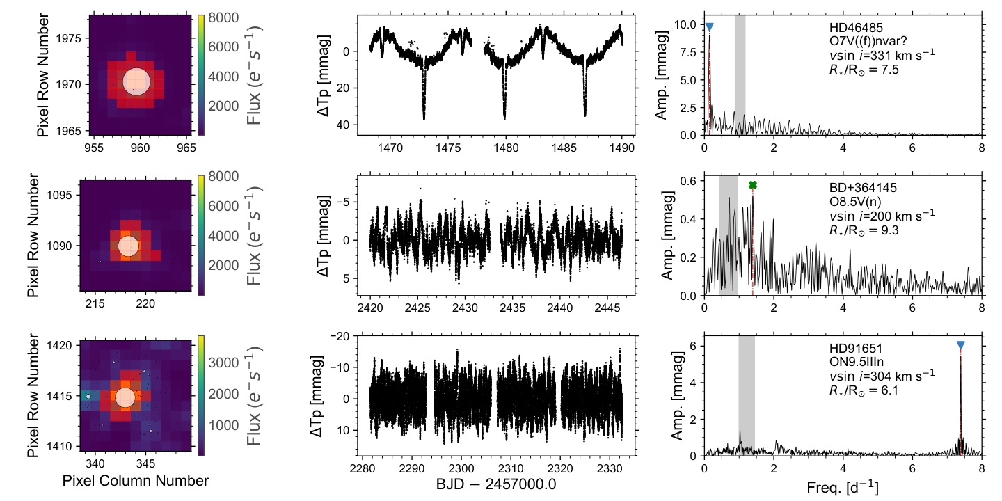
The TESS mission (Ricker et al. 2015) is delivering an enormously rich amount of high quality data for the asteroseismic analysis of large samples of stars covering a broad range of masses and evolutionary stages. In addition, the light curves delivered by TESS serve, among other things, for the detection of eclipsing binary systems (not necessarily transiting exoplanets) and the identification of specific variability patterns associated with the presence of spots at the stellar surface, variable winds, disks, or magnetospheres.
Our interest in getting access to the TESS lightcurves for a good fraction of our sample of fast-rotating O-type stars was mainly twofold. On the one hand, we wanted to identify signatures of eclipses in the photometric data, which could be indicating the presence of a companion not necessarily detected via time-series spectroscopy. On the other hand, by analyzing the resulting periodograms, we would be able to detect frequency patterns associated with fainter, less massive companions (i.e. Cep and SPB type pulsators, see Aerts et al. 2010 for an overview) whose identification would not be straightforward in the spectra.
An example of this latter situation was presented in Burssens et al. 2020, where it was shown that the periodogram obtained from the TESS lightcurve of the O7 V star HD 47839 – known to be 25 years period SB1 system (Gies et al. 1993; Gies et al. 1997). In addition, one of the longstanding standards for spectral classification clearly shows a high frequency peak (at 12.5 d-1), which most likely corresponds to a faint B-type companion and not to the bright O7 V star.
With these two ideas in mind, we first searched and extracted the TESS 2-min short-cadence data from the Mikulski Archive for Space Telescopes (MAST88 8 https://archive.stsci.edu/) for all stars in Table 1, if available (20 stars). We retrieve two light curves, the light curve extracted using simple aperture photometry (referred to as SAP) and the pre-conditioned light curve (Pre-search Data Conditioning Simple Aperture Photometry, PDCSAP). The latter has systematics removed that are common to all stars on the same CCD (Jenkins et al. 2016). Nonetheless, the SAP light curve may be preferable for certain stars as the pipeline is not optimised for OB stars.
By means of a visual comparison and based on predicted variability in the O-star regime, we selected the preferable light curve for each star. We additionally inspected the light curve aperture masks using the lightkurve software package (Lightkurve Collaboration et al. 2018) to rule out any contamination by nearby sources, large sector-to-sector mask variations, or the presence of oversaturated pixels. Light curves for which this was the case were removed from further consideration (1 star).
For stars with no available 2-min short cadence data, we extracted 30-min long cadence data using the lightkurve software package. If available (21 additional stars), we performed simple aperture photometry using a watershed method. That is, we included pixels with a light contribution within in flux of the light contribution of the central pixel of the source of interest. The extracted light curve was then detrended using principal component analysis, following Garcia et al. 2022. Again, problematic light curves were removed from further consideration (HD 216532).
The extraction procedure yielded 39 TESS light curves, all of which show some form of variability. This includes stochastic low-frequency variability, coherent pulsation modes, and rotational modulation and eclipses, which are in line with general findings for the O-star regime (Pedersen et al. 2019; Burssens et al. 2020). We show three examples of typical pixel maps, light curves and periodograms in Fig. 6. A detailed discussion about the photometric variability for each interesting target is presented in Appendix A. All information regarding photometric variability is presented in Table 1 (column ’Phot. var.’).
3.3 Compiling extra information from the literature
In addition to our own spectroscopic, photometric and astrometric analysis, we also performed a careful search in the literature for extra relevant information about our programme sample of stars. In particular, we wanted to know if any of the stars in our sample had been previously identified as a spectroscopic binary, as well as to compile any type of orbital and dynamical information resulting from any existing (more detailed) study of specific targets. Also, we gathered published information about close-by companions as resulting from high angular resolution surveys. Lastly, we looked for papers investigating whether any X-ray emission and/or magnetic feature had been identified among our sample of fast rotators.
3.3.1 Spectroscopic binaries
An important fraction of the stars considered in this work have been previously studied elsewhere. For example, 25 of them were included in the investigation of chemical abundances in fast-rotating massive stars by Cazorla et al. 2017a. The authors also searched for spectroscopic signatures of binarity in their sample. In addition, Trigueros Páez et al. 2021; Mahy et al. 2022 have studied several targets in common with our sample. A detailed discussion about the stars in common and some further notes about how this cross-match between our results and those obtained by previous authors have helpped us to fine-tune and/or reinforce our classification of stars in the sample of fast rotators between SB1, LPV, LPV/SB1? and LPV/SB2? (see column ’SB tag’ in Table 1) is presented in Appendix B.
3.3.2 Hunting for visual companions using high angular-resolution images
In order to check for any possible contamination of TESS data from other visually close stars to our programme targets, we searched for visual companions in different photometric surveys.
Taking into account that during the extraction of flux from the TESS full frame images, we applied a threshold mask, at the end we collected the flux from a different number of CCD pixels for each star (see Sect. 3.2.2). During the flux extraction, typically we chose the pixel with the greatest light contribution and select all pixels with light contributions within 8 of flux. Thus we collected the flux, typically between four and five pixels; however, in some crowded areas, the final mask of pixels consists of a larger amount of pixels. The size of TESS pixel is 21 arcsec, then we should take into account any source contamination within 2 arcmin (a bit more than five pixels).
This search for any possible contaminants was initiated with Gaia-EDR3 data. We identified all stars within 2 arcmin that demonstrate a difference in G magnitude smaller than 3 mag. Then, we complemented the available information in Gaia by performing an additional search in the Washington Double Star Catalog (Mason et al. 2001, WDSC,), which provides updated information about any identified companion in the literature. We also included results form specific high angular resolution surveys such as SMASH and Astralux, among others.
Generally speaking, we consider that if there is a nearby star with a difference in magnitude of less than 3 mag, the TESS lightcurves for a given target can be contaminated by the flux of a companion, which is not necessary gravitationally bound. This identification of the visual neighbours serves as a warning when extracting and interpreting the TESS photometric data. We note, however, that we also performed a thorough identification of potential contaminants which could be avoided when deciding on the final pixel mask used to extract the TESS light curve for each individual investigated target (see Sect. 3.2.2).
In the ’Potential contaminants’ column of Table 1, we indicated the outcome of this search. Namely, we indicated number of companions found within 1 arcmin, and between 1 and 2 arcmin which are separated by the symbol ’+’. More detailed information about the cases in which at least one visual component has been identified is summarised Table 6, including their angular distances, difference in magnitude, and the corresponding reference from which the information has been extracted.
3.3.3 Incidence of X-ray emission
Close compact companions to massive stars may lead to the emission of hard and bright X-rays, as demonstrated in X-ray binaries (Reig 2011, e.g.). Amongst our targets, 17 objects (including four SB1 systems) have been detected at X-ray wavelengths. For 14 targets, the estimates are available and have been published in various works. The corresponding flux ratio is listed in our Table 1 (see X-ray column). For the following targets, the measurements of X-ray fluxes are available in the literature, however, the estimates are not: HD 15137 (McSwain et al. 2010), HD 149452 (Fornasini et al. 2014) HD 46485 (Wang et al. 2007). Two additional ones, HD 76556 and HD 228841, are listed in the 4XMM source catalog. Their spectra were downloaded99 9 https://xcatdb.unistra.fr/4xmmdr10/index.html and analyzed within Xspec. All X-ray sources have a soft emission with 7, that is, their X-ray emission can fully be explained by the usual embedded wind-shocks of massive stars. There is therefore no indication for the presence of an accreting compact companion in any of our targets, nor of X-ray bright colliding winds arising in massive binary systems.
3.3.4 Incidence of magnetism
Another parameter that can be useful for a characterization of our sample is the presence of a magnetic field. The vast majority of O-type stars are known to be non-magnetic, but 7% of O-stars display strong, dipolar magnetic fields (Grunhut et al. 2017; Petit et al. 2019). Several theories have been proposed to explain this magnetism. In particular, Ferrario et al. 2009; Schneider et al. 2016 suggested that large-scale magnetism among massive stars originates in mergers. Because of the presence of a magnetic field in one component of Plaskett’s star, close binary interactions were also thought to be possible generators, but this assumption was discarded based on actual observations (Nazé et al. 2017).
Nevertheless, such channels (merging, binary interactions) may produce fast-rotating stars as an end product; thus, we decided to check available literature for the existence of magnetic field in our targets. Within the MiMeS survey (Grunhut et al. 2017; Petit et al. 2019), the Stokes profiles have been modelled for seven stars from our sample: HD 210839, HD 36879, HD 24912, HD 192281, HD 203064, HD 46056A, and HD 149757 – and none of these stars were found to be magnetic. Given the small number of studied stars, we could not draw any conclusion regarding the correlation between the existence of a magnetic field with binary or runaway statuses of our fast rotators.
4 Results and discussion
4.1 Preliminary considerations
In this section, we use the empirical information compiled in Tables 1 and 5 to evaluate the validity of the binary interaction scenario to explain the existence of a tail of fast rotators among Galactic O-type stars. To this aim, we compare some of the global properties of this working sample with those extracted from a complementary sample of stars with sin ¡ 200 km s-1.
Starting with the original sample of Galactic O-type stars investigated by Holgado et al. 2020; Holgado et al. 2022 and guided by the objective of trying to minimise as much as possible the potential effect of observational biases when performing this comparison, we decided to exclude all those stars fainter than V = 10 mag and/or located at a distance from the Sun larger than 3 kpc. After considering this filter – which was not only applied to the initial sample of 285 LS and SB1 stars, but also to the 113 SB2 systems detected by Holgado et al. 2020 --, we ended up with 179 and 47 LS or SB1 stars1010 10 In the case of the fast-rotating sample, the number also includes 2 stars classified as LPV/SB2?. having a sin below or above 200 km s-1, respectively, plus 93 SB2 systems (four of them having at least one of the components with sin 200 km s-1). Hereinafter, we refer to them as the slow- and fast-rotating samples, respectively.
4.2 The – sin diagram of Galactic O-type stars
Figure 7 depicts the distribution of the above-mentioned sample of 226 LS and SB1 stars in a vs. sin diagram. Both the and sin measurements for those targets in the slow-rotating sample are directly taken from Holgado 2019 and Holgado et al. 2022. In the case of the fast rotators (located to the right of the vertical grey shadowed band), we updated the estimates of these two quantities following the guidelines presented in Sections 3.1.2 and 3.1.3. As a result, we are also able to indicate the associated uncertainties in both sin and for the fast rotators.
Except for those stars with sin ¡ 200 km s-1 and ¡ 20 km s-1 (see reasoning below), wed use different colored symbols to identify the spectroscopic and eclipsing binaries, the periodic photometric modulation variables (including ellipsoidal and reflection modulations, labelled as ’periodic phot. mod.’), and those stars labelled as runaways. In the case of the fast-rotating sample, we take this information directly from Table 1. For the sake of the interest of the discussion, we have also performed a quick evaluation of the above-mentioned characteristics – following a similar strategy as in our main working sample – in the group of stars located in the upper left region of the diagram.
Red inclined lines depict the regions where is 5, 10, 15 of the sin value in the fast-rotating domain. These lines have been drawn to illustrate how intrinsic variability can lead to values of up to 15% of the corresponding sin . This spectroscopic variability does not only hamper the identification of low amplitude single-lined spectroscopic binaries among fast-rotating O-type stars1111 11 See also the case of O-stars and B supergiants with lower values of sin in Simón-Díaz et al. 2023. – especially when only a few number of epochs is available – but can also lead to a spurious identification of SB1 systems among these stars (see e.g. the case of HD 203064 in Sect. 3.3). However, based on our analysis we can suggest to use the threshold of ¿ 0.15 sin to separate the clear binaries from apparently single stars in the fast-rotating domain.
In the same vein, and following the guidelines presented in Simón-Díaz et al. 2023, we depict a horizontal grey shadowed band at 20 – 30 km s-1. This approximate threshold separates those targets below sin = 200 km s-1 which can be clearly marked as SB1 from those whose detected line-profile variability could originate from intrinsic variability. In particular, we mark all those stars with 30 km s-1 as SB1, but only those clearly detected as SB1 among the sin 200 km s-1 and 20 30 km s-1 sample after performing a more thorough evaluation of their spectroscopic binary status. The remaining targets (with 20 km s-1) are excluded from a similar study since most of them do not have enough number of epochs available for a reliable investigation of the spectroscopic variability.
Along this line of argument and taking into account the fact that the measured is expected to importantly depend on the number of available spectra when this number is low, we highlight stars for which we count on less than three spectra using empty circles. As depicted in Fig. 7, thanks to the specific observational efforts motivated by this study (see Sect. 2.2), the new compiled spectra have made us possible to avoid the low number of epochs caveat for a large percentage of stars in the fast-rotating sample (even reaching more than 5 epochs in most of them). However, as mentioned above, this is not the case for the sin 200 km s-1 sample. Therefore, in our working sample of fast rotators, we are quite confident that the measured is not going to importantly change by increasing the number of epochs and the percentage of identified SB1 systems will remain basically unaffected. On the contrary, in the low sin sample, those targets with less than five epochs (or even three) and estimates below 20 km s-1 could actually be unidentified SB1 systems. While this limitation will be taken into account for the discussion presented in Sect. 4.4 (where we compare the multiplicity statistics in the slow- and fast-rotating domains), it is interesting to also remark that there is a non-negligible number of stars (7) in the low sin sample with two to four epochs and a measured larger than 30 km s-1. Therefore, this fact seems to indicate that large amplitude SB1 systems are easily detected even with such a low number of epochs.
Grey inclined lines initiated in those data points corresponding to stars with ¿ 50 km s-1 represent deprojected values of both velocities assuming an inclination angle ranging from 90∘ to 50∘ (and perfect alignment between the spin and orbit axis). Filled gray squares along those lines represent the values at = 75∘ and 60∘, respectively. This analysis actually shows us that the inclination effect cannot significantly affect the statistics of spectroscopic binaries in the fast-rotating domain.
Globally speaking, in addition to the nine previously mentioned fast-rotating SB1 stars, we identify up to 38 clear single-line spectroscopic binaries with 20 km s-1 among the slow-rotating sample. Among them, and thanks to the availability of TESS data, we identify 3 eclipsing binaries (HD 36486, HD 152590, and BD+60∘498), as well as another 4 stars showing clear signatures of ellipsoidal (or reflection) modulation in their light curves (HD226868 -- aka Cyg X1 --, HD 12323, HD 53975, and HD 94024)1212 12 We refer the reader to Sect. 4.6 for a more detailed discussion about some of these targets (see also some information of interest in Table 7), along with those SB1 systems identified in the fast-rotating sample.. In addition, within the full sample of stars with sin 200 km s-1, there are 50 secure runaways (9 of them also tagged as SB1).
Inspection of Fig. 7 allows us to highlight several results of interest about the distribution of the global sample in the – sin diagram. Firstly, all SB1 systems in the fast-rotating domain have 30 km s-1, and are mainly distributed among two main groups – with high (120 – 170 km s-1) and low (30 – 60 km s-1) amplitudes, respectively (see also Fig.8). Indeed, a similar distribution is found in the slow-rotating sample, where a clear gap in is also detected. In addition, we confirm the result previously found by Holgado et al. 2022 that the percentage of SB1 stars with sin 300 km s-1 is very small, and basically zero for stars in the extreme tail of fast rotators. Further notes about the SB1 systems, along with an evaluation of the possible nature of the hidden secondary components (also using information from the literature and the TESS light curves) can be found in Sect. 4.6.
For completeness, we remind that, in addition to the mentioned difficulties to separate variations due to orbital motions in a binary system from intrinsic stellar variability in those stars with 20 km s-1, there are 40 stars in the low sin sample for which we have less than three spectra (i.e. 15% of the sample). This clearly explain why we do not see a normal distribution in the low domain of the corresponding histogram in Fig. 8 (contrarily to the case of the fast-rotating sample). Again, this will be taken into account when discussing the comparison of percentages of detected spectroscopic binaries in both samples.
Interestingly, all but two SB1 systems with 100 km s-1 are identified as eclipsing binaries. One of the stars in this subsample not identified as EB is Cyg X-1 (HD 226868, O9.7 Iab p var, sin = 95 km s-1), a well-known binary system (P5.59 d) hosting an accreting stellar-mass black hole (see Caballero-Nieves et al. 2009, an references therein); the other one is HD 130298 (O6.5 III(n)(f), sin = 167 km s-1, = 143 km s-1, P14.63 d) recently proposed by Mahy et al. 2022 to host a quiescent stellar-mass black hole.
If we now concentrate on the sample of SB1 stars with sin 150 km s-1 and 100 km s-1, there is only one star detected as eclipsing binary (HD 46485). Taking into account that the higher the measured sin , the most likely the binary system is observed at a high inclination (i.e. a configuration which favors the presence of eclipses if the orbital and rotational axes are aligned, as often assumed), those fast-rotating SB1 stars for which TESS do not show any signature of eclipses are potential candidates to host a compact object, as will be further discussed in Sect. 4.6. Other SB1 systems of interest (in both the slow and fast-rotating samples) for which we should be able to provide further information about the evolutionary nature of the hidden companion (see Sect. 4.6) are those stars identified to show ellipsoidal variability in the TESS light curves.
Lastly, most of the LS stars in the fast-rotating domain are runaways (see also Table 2), and only one fast-rotating SB1 star is also identified as runaway. The higher fraction of runaway stars among fast rotators was already highlighted in Sect. 3.2.1, while further insights about this result are presented in the next sections.
4.3 Comments on the global statistics of detected runaways
In Sect. 4.4, we discuss in more detail our findings about the multiplicity and runaway incidence among fast-rotating O-type stars. We also evaluate to what extent the obtained empirical results can be used to confirm or reject the binary evolution scenario proposed to explain the existence of a tail of fast rotators. Prior to this, we consider it of interest to briefly discuss the global statistics of detected runaway candidates among Galactic O-type stars1313 13 A more extensive study using the full list of OB-type stars in the ALS3 catalog (Pantaleoni González et al. 2021), comprising several thousand of targets and not excluding the SB2 systems, will be presented in Maíz Apellániz et al. (in. prep.). presented in Sect. 3.2.1 (see also Fig. 5).
Two important results can be derived from these global statistics. The first one is that the fraction of runaways we find is very high. Combining the fast and slow samples, there are 22% certain runaways and an additional 11% possible runaways. Those numbers indicate that up to 1/3 of the population of O-stars in the solar neighborhood may be runaways. These numbers are in rough agreement with the runaway fraction of 27% derived by Tetzlaff et al. 2011, but we note that their sample and methods are quite different. Their sample is dominated by B stars of lower mass than our stars and they used Hipparcos astrometry of much lower precision than that of Gaia-EDR3, so they were only able to assign probabilities to each star. On the other hand, the fraction is significantly higher than the value obtained by Maíz Apellániz et al. 2018, which was likely a consequence of the conservative nature of their methods.
The second result, of greater relevance for the present study, is that there is a significant difference between fast and slow rotators: for the first type we find that 35 – 50% are runaway stars, while for the second, we find a smaller number of 20-30%. This result confirms the finding of Maíz Apellániz et al. 2018 that Galactic runaway O-stars rotate significantly faster on average than their non-runaway counterparts and is also in agreement with the recent study by Sana et al. 2022, who found that the runaway population of (presumed) single O-type stars in the 30 Doradus region of the Magellanic Cloud presents a statistically significant overabundance of rapidly-rotating stars, compared to its non-runaway population.
This non-negligible difference in the percentage of runaways between the slow- and fast-rotating samples of Galactic O-type stars is somewhat expected if we assume as valid the proposal that binary interaction plays a dominant role in populating the tail of fast rotators. In this case, an important fraction of fast-rotating runaways (if not all) would be originated by the disruption of a post-interaction binary after the first core-collapse in the system. Indeed, Renzo et al. 2019 predicted that 50% of a population of high-mass interacting binaries will become a disrupted binary in which the initially less massive star is still on the main sequence. This percentage has been calculated following the information presented in Fig. 4 of Renzo et al. 2019 study; namely, starting from 78% of binary systems which do not merge and considering that 86% of those are predicted to be disrupted, 75% of them including a high-mass main sequence object after core-collapse of the companion. In constrast, since this ejection mechanism is not expected to be operating so efficiently among the slow-rotating sample, the associated runaways would be more likely produced by dynamical ejections resulting from a multi-body interaction in a dense cluster.
There is, however, one important caveat that must be taken into account in the argumentation above. One of the main outcomes of the extensive numerical study of the evolution of massive binary systems performed by Renzo et al. 2019 is that, despite the large percentage of disrupted binaries resulting from the simulations, only a small fraction of them is predicted to acquire peculiar velocities above 20 – 30 km s-1 (i.e. becoming a runaway from an empirical point of view). Therefore, if the estimations by Renzo et al. 2019 are correct, only a minor fraction of the detected runaways among the fast-rotating sample would come from the disruption of a binary.
Renzo et al. 2019 claim that this is a robust outcome of their simulations, also indicating that similar findings have been previously found by other authors (De Donder et al. 1997; Eldridge et al. 2011, e.g.). However, along the next sections, we will provide some arguments supporting the idea that this theoretical result seems to be in tension with our empirical findings. In particular, if all detected runaways in our sample of Galactic O-type stars would have been produced by dynamical ejections, there would no reason for the significantly larger fraction of runaways found between the slow and fast-rotating samples. Indeed, we note that even if we consider the most extreme runaways (with ¿ 50 km s-1), the fractions of stars with such tangential velocity are 19 in the fast-rotating domain and 8 in the slow-rotating domain (see Fig. 5). However, this is not the only argument and we present more details in the next section, where information about the detected binary status is also taken into account.
4.4 Multiplicity and runaway incidence amongst fast-rotating O-type stars
| sin | 200 km s-1 | —— | 200 km s-1 | ||||
|---|---|---|---|---|---|---|---|
| All | —— | All | Runaways | ||||
| # | % | —— | # | % | # | % | |
| Total | 268 | —— | 51 | 24 | 47 | ||
| SB1 | 35 | 13 | —— | 9 | 18 | 1 | 11 |
| SB2 | 89 | 33 | —— | 4 | 8 | 0 | … |
| LPV/SB2? | 0 | … | —— | (2) | (4) | 0 | … |
| LS | 143 | 54 | —— | 36 | 70 | 23 | 64 |
Table 2 summarises the number and relative percentage (with respect to the total number of stars in each group) of the various types of identified spectroscopic binaries within the slow- and fast-rotating samples. In addition, we indicate the number and percentage of runaways detected among the fast rotators1414 14 We remind that, in the quoted statistics, we have excluded those stars from the original sample studied by Holgado et al. 2020; Holgado et al. 2022 located at a farther distance than 3 kpc and/or which are dimmer than = 10 mag (namely: BD+60∘134, HD 124979, ALS12370).. Lastly, for reference purposes, we indicate that a preliminary estimation of the runaway fraction of stars in the slow-rotating SB1 and LS subsamples (based on the sample of stars considered in Section 3.2.1 and including ’possible runaways’) results in a similar percentage of 30%, respectively.
Concentrating first on the fast-rotating sample, it can be noticed that the sample is mainly dominated by likely single stars (70%), with a considerable smaller contribution of the single-lined spectroscopic binaries (18%) and only 8% comprising the confirmed SB2 systems. These numbers assume that the two stars identified as ”LPV/SB2?” are LS stars; however, if these were actually SB2 stars, the percentages of SB2 and LS stars would be slightly modified, but the main results remain valid.
In order to put these results in a wider context, we compare these numbers with the corresponding statistics for the stars with sin 200 km s-1. Before presenting our results and making comparisons with the fast-rotating sample, we must indicate that (as mentioned in Sect. 4.2) there is a sample of 22 slow-rotating stars (8.2% with respect to the total number of stars in the slow-rotating sample) for which we only have 1 spectrum available, plus another 18 (6.7%) with measurements based on two spectra. Although these stars will be labelled as LS hereinafter, there is some probability that some of them will be identified as SB1 or even SB2 systems when considering more epochs. Therefore, the percentage of SB1 and LS stars presented in the left column of Table 2 must be considered as lower (SB1 and SB2) and upper limits (LS), respectively. However, these percentages are not expected to vary by more than 7% (i.e. half of the sample with 1 – 2 epochs). In addition, since we have not explored in detail the SB1 status of those stars with sin 200 km s-1 and ¡ 20 km s-1, the percentages of SB1 and LS stars among the slow-rotating sample could again be somewhat larger (SB1) and smaller (LS), respectively, than those indicated in Table 2.
Taking all this into account, we can nevertheless extract interesting conclusions from inspection of the statistics presented in Table 2. The percentage of SB2 systems is smaller by a factor 4 in the fast rotating sample (with a difference between the relative percentages of the two samples of 25%). In contrast, the percentage of LS stars behaves in the opposite direction (with a minimum difference in percentage of 20% if we assume that no new SB1 systems in the low sin sample will be discovered whenever adding new epochs). Regarding SB1 systems, the percentage appears slightly larger among fast rotators. However, both percentages could become more similar if some SB1 stars are still hidden in our sample of stars with few epochs.
We can speculate that the observed fraction of SB2 systems in the slow-rotating domain is higher because these systems are pre-interaction binaries that have not yet evolved to a post-interaction binary system (including a fast-rotating O-type star orbiting a faint stripped star or a compact object), a merger, or a disrupted single runaway star after a supernova explosion event (de Mink et al. 2014, e.g.).
Alternatively, the explanation could be related to the difficulty to detect SB2 systems among stars with broad line profiles, or the fact that the majority of SB2 fast-rotating systems are short-period contact binaries (Penny et al. 2008, see for example HD 100213,) and this evolutionary phase is relatively short with respect to the other stages. However, we consider these two latter explanations as less probable than the abovementioned one. On the one hand, the quality and number of epochs of our compiled observations are good enough to have been able to detect the vast majority of SB2 systems (we note that only 2 out of 54 stars in our sample of fast rotators have survived as ’LPV/SB2?’). On the other hand, we have found four (out of 51 stars, i.e. 8%) clear SB2 systems, all of them having sin in the range of what is expected in terms of spin-orbit synchronization due to tides.
Another result that seems to further support the binary evolution scenario is the following. Even if future analyses of high quality data with a more extended multi epoch data set could aid to detect faint companions among the SB1 samples, if we add together the percentages of SB1 and SB2 systems, we end up with 26% and 46% of secured spectroscopic binaries among the fast- and slow-rotating samples, respectively. Even if we add the two fast rotators labeled as LPV/SB2? as spectroscopic binaries, the percentage of this type of systems among fast rotators is still considerably smaller than in the case of stars with sin 200 km s-1. In addition, as commented, some of the stars in our sample with 1 or 2 spectra could be discovered as SB1 systems in future investigations, thus increasing the difference in percentages even further.
Another point of interest refers to the statistic of runaway stars. As commented prevously( in Sections 3.2.1 and 4.3), 52% of the total sample of fast rotators are identified as runaways. Interestingly, all of them but HD 15137 (O9.5 II-IIIn, sin = 283 km s-1, = 44, SB1) are likely single stars, a result which, assuming the theoretical scenario proposed by de Mink et al. 2011, would support the dominance of the binary evolution scenario (after first core-collapse and supernova explosion) over the dynamical ejection (from a stellar cluster) channel (Perets & Šubr 2012, e.g.). As we discuss earlier in this paper, a significant difference in the observed fraction of runaways in the slow- and fast-rotating domain supports the scenario of disrupted binaries. However, we should note that the mentioned theoretical predictions (including Renzo et al. 2019, i.e. simulations) are sensitive to many initial conditions, including the star formation history rate, etc. Thus, if we do not know at which age we are observing the population of stars (the case of our sample), we cannot directly predict the exact fraction of runaway stars at a given stellar age.
From a different perspective, if we concentrate on the (36) fast-rotating and likely single stars, we can highlight two main groups: i) the runaways (64% of this subgroup versus 30% in the slow-rotating subgroup of these stars), as noted (see comments below), are expected to be mainly dominated by the products of a binary disruption event; and ii) the rest, which could either be the end-products of a merger event or binary systems for which we are not able to detect any clear spectroscopic binarity signature of a companion.
In reference to the runaway stars in the sample, there is still a possibility that some of them are fast-rotating single stars ejected from their parental stellar cluster by means of one or several dynamical interaction events during the star formation process (Maíz Apellániz et al. 2022). However, to distinguish the dynamical ejection from the binary supernova scenario for a sample of our stars is a tricky task that will require further work. An example of a star with peculiar kinematic properties is HD 149757, the origin of which is still under debate. It has been suggested that this star is a post-interaction binary (Villamariz & Herrero 2005; Renzo & Götberg 2021). It was also suggested that this star has been ejected after the supernova explosion of its massive companion (Tetzlaff et al. 2010; Kirsten et al. 2015). Also, the runaway status of HD 93521 possibly originates from a close binary interaction, and in addition to this, it is a possible merger product (Gies et al. 2022). Interestingly, we detected a single runaway SB1 system (McSwain et al. 2010, HD 15137,) amongst them: the only possibility to explain its existence would then be a dynamical ejection from a triple system in the past. In this context, it is interesting to note that HD 13268 and HD 15642 are runaways and members of the Perseus OB1 association (de Burgos et al. 2020). Thus, there is a possibility that they were dynamically ejected.
Regarding the LS fast rotators, the majority of stars in this group have ¡30 km s-1, thus if any hidden secondary component would be present, it should have a relatively small mass compared to the O-star. Indeed, we recall that in this rapid rotation regime, we expect to see the stars with the rotational axis almost perpendicular to the line of view. Moreover, considering (zero order approximation1515 15 It could most likely change following a donor’s supernovae kick.) that the orbit of fast-rotating star is expected to be perpendicular to the rotation axis, as usually assumed in case of short period or over-contact binaries (Fabry et al. 2022, e.g.), this implies that the velocity variations due to orbital motions should be close to their maximum values and would have been detected if the secondary masses were high enough. Therefore, it is only possible to have some hidden low-mass companion amongst them. One example is HD 46485, for which we could not detect any clear spectroscopic signature of binary motion with the available data set (five spectra) but TESS data show eclipses. In addition to this, de Mink et al. 2014 simulated the appearance of various binaries in terms of the orbital velocity of the components. According to these simulations, the systems with K 10 km s-1 ( 20 km s-1) could be either products of binary interaction (i.e. mergers or post-interaction binary systems) or effectively single stars. However, these simulations are valid for the general case of main-sequence objects without taking into account the rotation regime (presented in Sect. 4.7).
4.5 Distribution of the fast-rotating sample in the sHRD
The left panel of Fig. 9 depicts the location in the sHRD of our working sample of fast rotators, also including (for reference) the rest of the O-star sample investigated by Holgado et al. 2022, as well as the zero-age main sequence (ZAMS) line and the non-rotating evolutionary tracks computed by Ekström et al. 2012. Coloured symbols as in Fig. 7 are also used here to identify the various types of binaries as well as the runaway stars among the fast-rotating sample. For comparison, a similar sHRD diagram is depicted in the right panel of Fig. 9, this time including only the slow-rotating sample.
The first interesting result (Holgado et al. 2022, already pointed out by) is that all (9) fast-rotating SB1 systems are located below the 32 M⊙ evolutionary track, where a mixture of presumably single stars identified both as runaways (8) as well as targets without peculiar kinematical properties with respect to their local environment (7) can be also found. Additionally, the higher mass sample of fast rotators is basically dominated by LS runaway stars, with only 4 of the 18 stars in this region being detected as non-runaway LS stars. Also remarkable is that no fast rotators are found in the more evolved region of the MS in the higher mass domain.
The situation is completely different for the case of SB1 systems in the slow-rotating sample, where the distribution is more homogeneous along the whole O star domain (although with a somewhat larger relative percentage above the 40 M⊙ track). In addition, there is a clear concentration of runaway stars (mostly LS, but also some SB1) in the top right region of the diagram, where no fast-rotating stars are found. We should note that in a such comparison between fast- and slow-rotating domains we are dealing with target masses which are distributed uniformly; thus in our analysis and conclusions we do not have any bias toward specific mass domains. If we assume the scenario proposed by de Mink as valid, we could interpret the different distribution of runaways and SB1 systems in both panels in the following way. On the one hand, the fast-rotating higher mass runaways might be rejuvenated, spun-up gainers in a post-interaction binary system already disrupted after supernova explosion of the initially more massive companion. On the other hand, most of the more evolved, slow-rotating higher mass O-type runaways could be single stars which have been dynamically ejected from a cluster during the star formation process. Since there is no rejuvenation effect due to binary interaction, the probability of detecting more evolved O-stars among this latter sample is larger compared to the case of the fast-rotating sample. In the same vein, the SB1 systems also detected as runaways in the slow rotating sample could be interpreted as pre-interacting binaries which have been also ejected from their parental cloud during the star formation process – or as binary systems which previously were part of a triple system and in which one of the components exploded at some point as a supernova, hence producing the anomalous velocity (with respect to the local interstellar medium) of the detected SB1 system.
In summary, roughly speaking, we have detected two dominant sub-groups of fast-rotating stars in the sHRD, which likely represent two different stages of binary evolution: i) the least luminous SB1 systems and ii) presumably single luminous fast-rotating runaway stars coming from post-interaction systems. Such dominance of luminous runaway stars actually contradicts the simulations that are expected to have BHs as a companion of these systems, hence producing a smaller kick to the accretor (Sukhbold et al. 2016; Shenar et al. 2022a). To explain this distribution of runaways and SB1 systems will require detailed evolutionary modelling of each of these systems. In addition, these two main sub-groups are complemented with a third one, also mostly concentrated in the lower mass region of the O star domain, corresponding to the LS, non runaway stars, and representing 25% of the whole fast-rotating sample. This latter group could correspond to merger products or stars with relatively low mass (dim) post-interaction accretors which do not produce detectable variations nor eclipses in the TESS light curves. In this context, it is interesting to note that despite the superb quality of our spectroscopic dataset and the TESS photometry, the detection of small- signatures of orbital motion in a potential binary system and/or faint eclipses below 20 – 30 km s-1 and 5 – 20 mmag is hampered by the ubiquitous presence of intrinsic photometric and spectroscopic variability at the aforementioned level in the whole O-stars domain (Simón-Díaz et al. 2023, see also).
Interestingly, it is unlikely that some of the stars that are located on the upper part of the sHRD have some hidden SB1 components taking into account that almost all of them are classified as runaways. Thus, we do not expect to spot any other potential fast-rotating SB1 systems in that part of the sHRD, as a result, we do not have any observational bias on this sHRD distribution of fast rotators. As we have already pointed out, to explain the observed distribution of SB1 systems in the slow- and fast-rotating domain will require additional work in modelling the population of these systems. However, in any case it should serve as a constraint for further theoretical works that describe the evolution of binary fast-rotating systems.
4.6 Further notes about the properties of SB1 systems and the characterization of hidden companions
| Target | HD 163892 | HD 308813 | HD 37737 | HD 152200 | HD 165246 | HD 15137 | HD 165174 | HD 52533 | HD 46485 |
|---|---|---|---|---|---|---|---|---|---|
| SpC | O9.5 IV(n) | O9.7 IV(n) | O9.5 II-III(n) | O9.7 IV(n) | O8 V(n) | O9.5 II-IIIn | O9.7 IIn | O8.5 IVn | O7 V((f))nvar? |
| sin [km s-1] | 201 | 205 | 209 | 210 | 254 | 283 | 299 | 312 | 334 |
| [km s-1] | 83.5 | 41.5 | 156.5 | 32.0 | 126.0 | 44.0 | 59.5 | 166.0 | 29.5 |
| [kK] | 32.8 | 31.8 | 30.0 | 30.4 | 35.9 | 30.3 | 30.2 | 35.2 | 36.1 |
| log() | 3.68 | 3.52 | 3.8 | 3.63 | 3.62 | 3.84 | 3.86 | 3.6 | 3.74 |
| [] | 9.3 | 6.9 | 10.3 | 6.8 | 7.8 | 10.7 | 10.7 | 7.9 | 7.5 – 11 |
| log(/) | 4.95 | 4.65 | 4.88 | 4.54 | 4.96 | 4.94 | 4.93 | 4.92 | 4.93 |
| [M⊙] | 19 | 12.3 | 12.4 | 8 | 22 | 13 | 15 | 22 | 17 |
| sin / | 0.3 | 0.3 | 0.4 | 0.4 | 0.4 | 0.5 | 0.6 | 0.4 | 0.5 |
| Runaway tag | n | n | n | n | n | y | n | n | n |
| EB tag | – | ? | EB | RM | EB | n | – | EB | EB+RM |
| P [d] | 7.8 | 6.3 | 7.8 | 4.5c | 4.6b | 55.3 | 23.9 | 22.0 | 6.9c |
| [km s-1] | 41 | 32 | 70 | 23c | 53b | 16 | 30a | 88 | 15c |
| 0.04 | 0.38 | 0.38 | 0.17c | 0.03b | 0.66 | 0.16 | 0.27 | 0.01c | |
| [M⊙] | 0.0708e | 0.0198 | 0.2224 | 0.004c | 0.071b | 0.0092 | 0.0313 | 1.02d | 0.002 – 0.00091c |
| [∘] | 70 | 25 | 75 | (45)c | 84b | 45 | (45) | 90 | 80 – 75c |
| [km s-1] | 60 | 55 | 67 | 76 | 86 | 10 | 23 | 18 | 55 |
| [km s-1] | 215 | 485 | 215 | 295 | 255 | 400 | 420 | 310 | 340 |
| Rough mass estimation of the hidden secondary companion ( [M⊙]) | |||||||||
| From , , | 3.5 | 4.1 | 4.1 | 1.0 | 3.6 | 1.8 | 3.1 | 10.0 | 0.9 |
| From , , | 3.4 – 4.2 | 5.8 – 7.5 | 5.6 – 7.2 | 1.7 – 2.3 | 3.4 – 4.5 | 2.6 – 3.3 | 4.8 – 6.2 | 11.2 – 14.1 | 1.0 – 1.3 |
Notes: Information presented in the top half of the table has been extracted from Tables 1 and 5 in this paper. The orbital parameters presented in the second half of the table have been mainly compiled from Mahy et al. 2022 except from those quantities conveniently specified, extracted from: a This work; b Johnston et al. 2021; c Simón-Díaz et al. (in prep.) and Nazé et al. 2023; d Trigueros Páez et al. 2021; e Cazorla et al. 2017a. Values of sin /, , , , , and have been rounded to 0.1, 0.1 d, 1 km s-1, 0.01, 1 km s-1, and 5 km s-1, respectively.
Table 3 provides a summary of all information of interest for the nine definitely confirmed fast-rotating SB1 systems1616 16 See also Table 7 for some info on those SB1 in the low sin sample identified as eclipsing binaries and/or ellipsoidal variables.. In addition to the information obtained by ourselves for the purpose of this paper (top half of the table), we compile additional information about several orbital parameters (period, semi-amplitude of the curve, inclination, eccentricity, and mass function; namely, , , , , and , respectively) in the middle part of the table. The information described above is also complemented with some estimates of the surface velocity the star would have if the spin and orbit were synchronised (, as well as the quantity sin / (were is the critical rotational velocity), and , namely, the estimated equatorial velocity of the star assuming the inclination angle quoted in the table. Lastly, at the bottom, we provide two estimations of the individual mass of the hidden companions by assuming that the mass of the primary is given by a) the spectroscopic mass resulting from the estimated surface gravity (corrected for centrifugal forces) and the radius derived taking into account the apparent magnitude of the star, its distance, and extinction, as well as b) an approximated evolutionary mass (25 5 M⊙), as obtained from the location of the fast-rotating SB1 sample in the sHRD (see left panel in Fig. 9).
Most of the information on the orbital parameters quoted in the table have been extracted from the recent study by Mahy et al. 2022, except for three stars; one of them (HD 152200) is a newly discovered SB1 system, while HD 46485 is confirmed ’bona fide’ SB1 system and the third one (HD 165246) has been studied in detail by Johnston et al. 2021.
To first give a global overview of the properties of the sample, regarding the amplitude of variability and the detection of eclipses and/or ellipsoidal modulation in the TESS light curves we have: (i) three large-amplitude ( 100 km s-1) SB1 binaries, all of them being also eclipsing binaries (HD 37737, HD 165246, and HD 52533); (ii) four small amplitude ( 50 km s-1) SB1 binaries, including one eclipsing, non-runaway system (HD 46485), two non-runaway targets whose TESS light curves show periodic photometric modulations (HD 308813 and HD 152200), and one runaway star with no signatures of eclipses or ellipsoidal variability (HD 15137); (iii) two intermediate amplitude non-runaway SB1 binaries for which there is no TESS data available (preventing us from evaluating their EB/EV status, HD 163892 and HD 165174).
If we pay attention to the orbital periods of the systems, we find two main groups, one of them including six systems with orbital periods in the range 4.5 – 8 d (most of them also detected as eclipsing binaries and/or ellipsoidal variables), plus another one comprising three systems with a somewhat longer period (20 – 50 d). In this latter group, there is one eclipsing binary, one runaway star, and a third target tagged neither as runaway nor as eclipsing binary or ellipsoidal variable. Interestingly, there does not seem to be any correlation between and within stars in any of these two main groups.
The first conclusion we can extract by inspecting the information compiled in Table 3 (more specifically, by comparing the measured sin with the estimated equatorial velocities assuming spin-orbit synchronization) is that it is quite unlikely that the spectroscopically detected components of these nine fast-rotating SB1 systems have acquired their relatively large equatorial velocities through tidal effects, leaving again the binary interaction channel as the most probable one.
According to theory, the dim (hidden) companion of a post-interaction high-mass binary can be either a compact object (Langer et al. 2020; Mahy et al. 2022, e.g. black holes and neutron stars, BH/NS; see) or a stripped helium star or subdwarf object (de Mink et al. 2013; Shao & Li 2014; Götberg et al. 2018, e.g.).
Among the nine investigated SB1 systems, there are five targets for which the presence of a black hole or neutron star can be discarded. This includes the four stars for which two clear eclipses are detected in the TESS light curve, plus1717 17 We remind that, by the time of submission of this paper, there was no TESS light curve available for HD 163892; hence, we could not evaluated if this system is also an eclipsing binary. HD 163892, for which Mahy et al. 2022 claim to have identified spectroscopically the secondary by means of a spectral disentangling technique1818 18 This is also the case for HD 52533.. Among the remaining four stars, there are two targets for which TESS data shows potential signatures of periodic photometric modulation (HD 308813 and HD 152200), a third one detected as a runaway SB1 system with an orbital period of 55 days and a quite large eccentric orbit (HD 15137), and a fourth target (HD 165174, 24 d, 0.16) not detected as runaway, but for which we do not have TESS data available to evaluate its photometric behaviour. All but HD 152200 have been investigated in detail by Mahy et al. 2022, who do not propose any of them as candidates to host a quiescent stellar mass black hole. Additionally, they show that in case the secondary would have a mass exceeding 3 M⊙ (see last 2 rows of Table 3), it would have been detected in the spectrum using their disentangling technique.
HD 308813 displays clear phase-locked modulations in flux and radial velocities, however, they are difficult to interpret especially in view of the low number of spectroscopic observations. Nevertheless, no evidence indicate that this binary system hosts a black hole or neutron star. Further characterisations of this system will require more spectroscopic observations.
Another situation occurs in the case of the two newly confirmed SB1 systems HD 152200 and HD 46485. The shape of their light curve shows the typical behavior of a binary system in which half of the stellar surface of the cooler component is illuminated by the hotter star (reflection modulation; i.e. maximum and minimum flux at conjunction moment). This leaves us with HD 165174 as the only possible fast-rotating O-type star in our sample for which the presence of a quiescent compact object cannot be definitely ruled out (pending the acquisition of new TESS data or high-quality ground-based photometry and further ultraviolet observations).
Lastly and rather importantly, our only fast-rotating SB1 system also detected as a runaway (HD 15137) deserves further attention. This star was investigated in detail by McSwain et al. 2010, finding that it may contain an elusive neutron star, in the ejector regime or a quiescent black hole with conditions unfavorable for accretion at the time the XMM observations used in that study were obtained. Mahy et al. 2022 also included this star in their search for quiescent O+BH/NS systems, estimating the mass of the hidden companion to be in the 1 – 6 M⊙ range (with a more probable mass of 2.5 M⊙) and indicating that they could have identified this dimmer companion in the spectra if it would have a mass above 3 M⊙ while the star is not actually detected. Our estimated mass of the secondary also points to this boundary limit which leaves the exact nature of the hidden companion still elusive.
As commented in Sect. 4.2, there are another four stars among the low sin sample that deserve further attention in this context. These refers to those SB1 stars with sin 200 km s-1 for which we have detected signatures of ellipsoidal (or reflection, depending on the considered orbital period of the system) variability ion the TESS light curves. One of them is HD 226868 (aka Cyg X-1), a well studied binary system comprising a late-O supergiant orbiting an accreting stellar-mass black hole (see Caballero-Nieves et al. 2009, an references therein). Another two are: HD 12323 (ON9.2 V, sin = 121 km s-1, = 58 km s-1) and HD 94024 (O8 IV, sin = 162 km s-1, = 54 km s-1). By combining the available and TESS data we can confirm that the period of these binary systems are 1.92 and 2.46 days, respectively, and that the folded light curves correspond to ellipsoidal modulation (Mahy et al. 2022, as also pointed out by). Interestingly, these authors claimed as unlikely that any of these two systems host a stellar mass black hole by considering that the higher mass of the hidden companion is obtained when assuming spin-orbit synchronization. However, the situation changes if, instead of tidal synchronization and in view of the detected ellipsoidal modulation, we assume that these stars actually have a much faster equatorial velocity, reaching values on the order of /0.4 – 0.6, as in the case of the other SB1 system in our fast-rotating sample (see Table 3). In this case, the estimated masses of the hidden companion would be in the range 3 – 6 M⊙ and 2.5 – 5 M⊙, respectively; hence, leaving the door to be considered as binary systems hosting a stellar-mass black hole (or at least a neutron star) still open.
Regarding HD 53975 (O7.5 Vz, sin = 179 km s-1, = 47 km s-1), the last star in this group, we do not have yet enough epochs to check if the orbital period is 12.5 or 6.25 days. Therefore, more measurements are needed to decide if the photometric variability detected in the TESS light curve is associated with ellipsoidal or reflection modulation, an evaluate the evolutionary nature of the hidden companion.

4.7 Comparison with theoretical predictions
As we have pointed out, based on the observational properties of the investigated sample of fast rotators, it is likely that the vast majority of them can be assumed to be post-interaction binary products. Using the information presented in Table 2, Fig. 10 provides a global overview of the main characteristics of our sample of 51 Galactic O-type stars with sin 200 km s-1. In particular, it highlights the relative percentage of presumably single stars and spectroscopic binaries, as well as of detected eclipsing binaries and runaways in each subsample. As we can see from Fig. 10, only 25% of all fast rotators are likely single stars – and not runaways. These targets could be mergers, following the theoretical predictions regarding the origin of rapid rotators of de Mink et al. 2013. The detailed characterization of fast rotators presented in this work is a crucial testbed for further theoretical studies of stellar evolution. The next step is therefore to compare model predictions with our observational results.
Recent simulations of OB binary system configurations by Langer et al. 2020 suggest that fast-rotating systems with a range of orbital velocities from 50 km s-1 (i.e. 100 km s-1, case A – donor is on the main sequence) to 100 km s-1 (i.e. 200 km s-1, case B – donor is evolving to the Red Giant phase) most likely have black holes as companions (see Fig. 6 in the cited paper). These simulations can be placed in terms of rotational velocity as well. Thus, theoretically, the OB+BH systems have a higher probability to be detected with equatorial rotational velocity ()100 km s-1, 100 km s-1 (slow-rotating domain) and 500 km s-1, 50 km s-1(fast-rotating domain, C. Schürmann, private comm.). As we discuss in Sect. 4.6, we did not detect any SB1 system with sin ¿350 km s-1. However, we did detect LS runaway stars with sin 400 km s-1 that could be proven to be disrupted systems following a supernova explosion. From another aspect, according to Fig. 7, the majority of SB1 systems with possible or confirmed BH companions are located in the slow-rotating domain at 10050 km s-1. These observational results should be taken into account in future theoretical works regarding the prediction of the existence of OB+BH systems.
Moreover, within the present work, we also aimed to evaluate the observational appearance of fast-rotating O-type stars based on recent theoretical predictions. To do so, we have used the synthetic stellar populations from the Binary Population And Spectral Synthesis v2.2.1 results (Eldridge et al. 2017; Stanway & Eldridge 2018) to estimate the expected properties of fast rotators in various O-star subpopulations, i.e. SB1, SB2 and singles. We use the fiducial BPASS population, this includes a mix of single stars and binary stars as described by Moe & Di Stefano 2017, although the majority of O-stars are in binary systems. We also use prescribed initial mass ratio and period distributions from the same source. The applied IMF is Kroupa et al. 1993 with an upper mass limit of 300 M⊙.
BPASS stellar models calculate the detailed structure and evolution of each star in sequence using a custom version of the Cambridge STARS code. First, it evolves the more massive primary in detail and approximates the secondary evolution using the stellar evolution equations of Hurley et al. 2000. It then calculates the evolution of the secondary in detail either as a single star or a binary with a compact companion. Thus, in making synthetic O-star sub-populations we use the following constraints to put stellar models into each group. We classify an O-star as having kK, a luminosity of and a surface hydrogen mass fraction above 0.2.
In what follows, we use specific definitions of SB1, SB2, and single stars. It assumes that the SBs are all post-interaction products. This is an extreme assumption but it provides important constrain on what binary interaction can produce and, thus, help to interpret the observational results.
Indeed, to accurately predict the number of SB2 stars expected from an observation survey is difficult. It is a complex interplay between the relative luminosity of the two stars but also whether the orbital period is short enough that radial velocity variations can be observed. In the clearest cases of similar luminosities and short periods, a SB2 identification is simple. Actually, we performed the simulations of the line-profile appearance by varying the flux contributions of the secondary component with different sin regimes of the primary component (see our simulations in Fig. 15). It becomes more difficult as the luminosities become more different and the periods become longer (i.e. smaller orbital velocities). In some ways determining if a star is a SB2 or SB1 depends more on the luminosity, while the LS sample will have some wide SB1 binaries. However, the error introduced by not taking all these factors into consideration is on the order of a few % as the majority of our LS arise from unbound binaries and single stars. A true detailed reproduction of the observed population, taking into account all the complex selection effects, is beyond the scope of this paper. In a present work, for our BPASS modelling we used the following definitions. The SB2 O-stars are taken from the initial models when both stars in the binary are O-stars or when the luminosities of the two stars are both within an order of magnitude. The SB1 are all stars in binary systems that do not count as an SB2 system. This includes systems where the secondary star is an O-star and the primary is the post-binary interaction donor star or a compact remnant. It also includes systems with an O star as primary and a secondary being a lower mass main-sequence star with a difference in luminosity greater than an order of magnitude. The single O-stars are either O-stars that were originally single (a small number), post-interaction binaries after a merger event or the initially less massive companions in a binary system that become unbounded after the supernova explosion of the star that was the primary when the system originated.
Current BPASS models do not include a detailed model of rotation. However, rapidly rotating O-stars are identified by tagging stellar models where the accretor increases its mass by more than 5% of its initial mass or those O-stars that have merged with their companion. In both cases, such stars will be expected to be rapidly rotating and be far above the threshold assumed in our observations (de Mink et al. 2013). While this is an approximate treatment, it allows us to estimate a lower limit to the population of rapid rotating O-stars. For example, rotation will extend the life of the O-star and we did not include models in which there is a lesser degree of mass transfer, but where stars will still be boosted up the the extent that they end up being observed as rapidly rotating. However, these are second-order effects and our predictions provide a robust estimate of the importance of mass-transfer as the source of rapid rotation. In varying the parameters, we have chosen to define the synthetic O-star populations, such as the magnitude difference for SB2 or SB1 systems, leading to an uncertainty in our predicted sub-populations on the order of a few percent of the population for each predicted value.
We used two metallicity models appropriate for solar metallicity: and 0.020. This allows for variations and uncertainties in the abundances of the observed stellar population. Amongst the modelled O-star populations, the fraction of fast rotators is 20-25% among, which we can emphasise the next sub-groups of targets depending on their binary status: (i) LS: 70% (among which 14% are runaways and 11% are walkaways); (ii) SB1: 15% (among which 9% are runaways, and 3% are walkaways); (iii) SB2: 15%.
The fraction of runaway stars was calculated by considering the impact of the first supernova. For single star runaways, these are assumed to be O-stars whose binaries have been unbound in the first supernova, while the SB1 runaways are all systems that have experienced a supernova, forming a neutron star and not a black hole.
To calculate the O-star velocities, we modelled the effect of the primary star’s supernova on the binary. We used the formalism of Tauris & Takens 1998 and Tauris et al. 1999, and assuming the neutron star receives a kick from the Hobbs et al. 2005 distribution. The O-star velocities are essentially the pre-supernova orbital velocity of the O-star in cases where stars are unbound. We estimate that the number of systems where a kick will be strong enough to accelerate the accretor up to 30 km s-1 is only 3% (i.e. walkaways) and 9% is the fraction of runaways with velocity more than 30 km s-1 of SB1 systems (or approximately 2% of the entire rapid rotator population). For the single stars, we estimate the number of walkaways to be 11% and 14% of runaways with a velocity of more than 30 km s-1(in total this is 18% of the entire population). As we may notice, according to our simulations and observations, the fast rotators will be more likely to be runaways than walkaways.
Schematically, these results are presented on the right panel of Fig. 10 with the same labels as on the left panel, to ease comparison with the observational results. These values are on the same order as the rates that we observationally inferred, especially if we will take into account that some of the ’LPV/SB2?’ systems may be shown to be LS objects after all. This good agreement implies that the majority of fast-rotating stars appear to be LS (de Mink et al. 2011) and mass transfer is the primary physical process responsible for creating rapid rotation, as already suggested by de Mink et al. 2013. This is also in line with expectations from Haemmerlé et al. 2017 and Bodensteiner et al. 2020 regarding Be stars, that such a rapid rotation would be difficult to be already present at birth. We note that the prediction here of the number of mergers becoming rapid rotators (i.e. 52%) should be treated as an upper limit. A recent work by Schneider et al. 2019 suggests that merger products may be highly magnetic. This would then lead to a rapid spin down of such objects, suggesting some merger products may, in fact, be slow-rotating (Schneider et al. 2020).
BPASS provides further detail on the nature of SB1 systems. In these models, a SB1 is any binary system for which there is only one O-star in the binary. If both stars are main-sequence stars, this occurs when the primary is 0.5 dex more luminous than the secondary since the secondary is not an O-star in this case. In addition to the case above, as SB1 systems BPASS considers any O-type binaries with compact remnants (NS) as secondaries. Thus, BPASS yields: (i) the fraction of SB1 systems with a rapidly rotating star is about 6% of all O-type SB1 systems; (ii) for SB1 systems with a slow-rotating O-star, 92% are the pre-interacting stars of their systems, 5% are systems in which the O-star was initially the secondary star but its status changed due to mass transfer, and 3% are O-stars paired with a compact remnant; (iii) for SB1 systems with a fast-rotating O-star, mass transfer has occurred in all cases (from the definition of fast rotators in the models, see above). The fraction of O-star paired with a compact remnant is about 84% of the systems, while the fraction of the O-star paired with a post-mass transfer object (e.g. stripped star) is 16%.
The illustration of these results is presented in Fig. 16. A more detailed investigation of the SB1 system’s companions requires the combination of photometric and radial velocity curve property studies in order to reconstruct the orbit of the system that could give a hint about which of the two predicted subgroups of companions we are dealing with.
Given that these BPASS models explain many other varied observations of massive stars and related transients (Eldridge et al. 2017; Stanway & Eldridge 2018; Massey et al. 2021; Briel et al. 2022, e.g.), it is positive to see that the same fiducial population can provide estimates that are of the same order as the observed population. However, the agreement is not perfect and, thus, refinements to the models of massive O-stars are required. Especially it concerns the predicted fraction of runaway stars – the predicted runaway population includes runaways caused by supernova only – if the dynamical runaways were included the total runaway population could be significantly increased (Eldridge et al. 2011, see e.g.).
5 Conclusions and future prospects
In the present work, we studied a statistically meaningful sample of several tens of Galactic, fast-rotating O-type stars. By analyzing their multiplicity and runaway status, we can draw the following main conclusions:
- •
The fraction of runaway stars among fast-rotating O-stars is 33-50%, which is significantly higher than for slow rotators (20-30%). Notably, we have detected several fast-rotating runaways with significant high tangential velocity, that is, ¿50 km s-1.
- •
The fraction of SB1 systems in the fast-rotating domain is 18. If we assume that they are all post-interaction binaries, the comparison with models indicates that they are products of mass-transfer with a secondary component which can be a compact remnant (black hole or neutron star) or a post-mass transfer object (stripped helium star or subdwarf object).
- •
The fraction of SB2 systems among O-type fast rotators is about 8-12 which is significantly lower than in the slow-rotating domain 33. Most likely, this statistic indicates how binary systems are evolving from slow-rotating pre-interacting systems to the post-interaction system with rapid rotation. In addition, to support this hypothesis, we detected that the fraction of SB1 systems in the fast-rotating domain (18) is slightly higher than the fraction of these systems in the slow-rotating domain (13).
- •
We found a couple of intriguing fast-rotating SB1 systems that will require further detailed investigation, namely: HD 152200 and HD 46485, which possibly host a post-interaction low-mass companion (compact remnant or stripped star or subdwarf object), as well as HD 308813, which will require further characterization.
Taking into account the fact that single fast-rotating runaway stars are post-mass transfer systems without a secondary component, whereas SB1 systems are actually post-interaction systems too, we can conclude that the majority of fast-rotating O-type acquired their fast rotation via mass-transfer ( 65%). In addition, some fast rotators are possibly passing by tidal synchronization scenario as the overcontact SB2 systems ( 10%). The rest of the stars could be considered as merger products (e.g. HD 93521), although their exact fraction remains elusive. Indeed, the issue of how to distinguish the population of mergers from effectively single fast rotators (if any) or from fast rotators with hidden companions remains an open question.
The last point that we did not cover in this work is the study of the chemical evolution of fast-rotating stars which will require further investigation. We did not perform a detailed investigation for all fast rotators in our sample, however, helium and nitrogen abundances are available from the literature (Cazorla et al. 2017b; Holgado 2019). Notably, Cazorla et al. 2017b showed that it is possible to reproduce the stellar atmospheric parameters and abundances for half of their sample of fast-rotating stars by using single-star evolutionary models but others require binary evolution models. In order to perform a detailed investigation of the current evolutionary stages of fast-rotating stars from the chemical composition point-of-view, we need to derive the CNO abundances for the full sample of targets.
Acknowledgements.
We thank the referee, Tomer Shenar, for an extremely constructive and respectful report which has helped us to improve the first version of the paper, and also provided interesting ideas for future development. N.B. acknowledge support from the postdoctoral programme (IPD-STEMA) of Liege University. N.B., S.S-D, G.H and A.H. acknowledge support from the Spanish Ministry of Science and Innovation (MICINN) through the Spanish State Research Agency through grants PGC-2018-0913741-B-C22, PID2021-122397NB-C21, and the Severo Ochoa Programe 2020-2023 (CEX2019-000920-S). This work has also received financial support from the Canarian Agency for Economy, Knowledge, and Employment and the European Regional Development Fund (ERDF/EU), under grant with reference ProID2020010016. This paper is based on observations made with the Nordic Optical Telescope, operated by NOTSA, and the Mercator Telescope, operated by the Flemish Community, both at the Observatorio del Roque de los Muchachos (La Palma, Spain) of the Instituto de Astrofísica de Canarias. Based (partly) on data obtained with the STELLA robotic telescopes in Tenerife, an AIP facility jointly operated by AIP and IAC. This work has made use of data from the European Space Agency (ESA) mission Gaia (https://www.cosmos.esa.int/gaia), processed by the Gaia Data Processing and Analysis Consortium (DPAC, https://www.cosmos.esa.int/web/gaia/dpac/consortium). Funding for the DPAC has been provided by national institutions, in particular the institutions participating in the Gaia Multilateral Agreement. J. M. A., G. H. and M. P. G. acknowledge support from the Spanish Government Ministerio de Ciencia e Innovación through grant PGC2018--B-C22. Y.N. acknowledge support from the Fonds National de la Recherche Scientifique (Belgium), the European Space Agency (ESA), and the Belgian Federal Science Policy Office (BELSPO) in the framework of the PRODEX Programme (contract linked to XMM-Newton).References
- Abdul-Masih et al. (2021) Abdul-Masih, M., Sana, H., Hawcroft, C., et al. 2021, A&A, 651, A96
- Aerts et al. (2010) Aerts, C., Christensen-Dalsgaard, J., & Kurtz, D. W. 2010, Asteroseismology
- Aerts et al. (2014) Aerts, C., Simón-Díaz, S., Groot, P. J., & Degroote, P. 2014, A&A, 569, A118
- Aldoretta et al. (2015) Aldoretta, E. J., Caballero-Nieves, S. M., Gies, D. R., et al. 2015, AJ, 149, 26
- Bailer-Jones et al. (2021) Bailer-Jones, C. A. L., Rybizki, J., Fouesneau, M., Demleitner, M., & Andrae, R. 2021, AJ, 161, 147
- Banyard et al. (2022) Banyard, G., Mahy, L., Sana, H., et al. 2022, arXiv e-prints, arXiv:2210.07149
- Barbá et al. (2017) Barbá, R. H., Gamen, R., Arias, J. I., & Morrell, N. I. 2017, in The Lives and Death-Throes of Massive Stars, ed. J. J. Eldridge, J. C. Bray, L. A. S. McClelland, & L. Xiao, Vol. 329, 89–96
- Bhatt et al. (2010) Bhatt, H., Pandey, J. C., Kumar, B., Sagar, R., & Singh, K. P. 2010, New A, 15, 755
- Blaauw (1961) Blaauw, A. 1961, Bull. Astron. Inst. Netherlands, 15, 265
- Bodensteiner et al. (2020) Bodensteiner, J., Shenar, T., & Sana, H. 2020, A&A, 641, A42
- Briel et al. (2022) Briel, M. M., Eldridge, J. J., Stanway, E. R., Stevance, H. F., & Chrimes, A. A. 2022, MNRAS, 514, 1315
- Briquet et al. (2011) Briquet, M., Aerts, C., Baglin, A., et al. 2011, A&A, 527, A112
- Burssens et al. (2020) Burssens, S., Simón-Díaz, S., Bowman, D. M., et al. 2020, A&A, 639, A81
- Caballero-Nieves et al. (2009) Caballero-Nieves, S. M., Gies, D. R., Bolton, C. T., et al. 2009, ApJ, 701, 1895
- Cantat-Gaudin & Brandt (2021) Cantat-Gaudin, T. & Brandt, T. D. 2021, A&A, 649, A124
- Cazorla et al. (2017a) Cazorla, C., Morel, T., Nazé, Y., et al. 2017a, A&A, 603, A56
- Cazorla et al. (2017b) Cazorla, C., Nazé, Y., Morel, T., et al. 2017b, A&A, 604, A123
- Chini et al. (2012) Chini, R., Hoffmeister, V. H., Nasseri, A., Stahl, O., & Zinnecker, H. 2012, MNRAS, 424, 1925
- Cohen et al. (2021) Cohen, D. H., Parts, V. V., Doskoch, G. M., et al. 2021, MNRAS, 503, 715
- Conti & Ebbets (1977) Conti, P. S. & Ebbets, D. 1977, ApJ, 213, 438
- De Becker & Raucq (2013) De Becker, M. & Raucq, F. 2013, A&A, 558, A28
- de Burgos et al. (2020) de Burgos, A., Simon-Díaz, S., Lennon, D. J., et al. 2020, A&A, 643, A116
- De Donder et al. (1997) De Donder, E., Vanbeveren, D., & van Bever, J. 1997, A&A, 318, 812
- de Mink et al. (2011) de Mink, S. E., Langer, N., & Izzard, R. G. 2011, in Active OB Stars: Structure, Evolution, Mass Loss, and Critical Limits, ed. C. Neiner, G. Wade, G. Meynet, & G. Peters, Vol. 272, 531–532
- de Mink et al. (2013) de Mink, S. E., Langer, N., Izzard, R. G., Sana, H., & de Koter, A. 2013, ApJ, 764, 166
- de Mink et al. (2014) de Mink, S. E., Sana, H., Langer, N., Izzard, R. G., & Schneider, F. R. N. 2014, ApJ, 782, 7
- Ekström et al. (2012) Ekström, S., Georgy, C., Eggenberger, P., et al. 2012, A&A, 537, A146
- Eldridge et al. (2011) Eldridge, J. J., Langer, N., & Tout, C. A. 2011, MNRAS, 414, 3501
- Eldridge et al. (2017) Eldridge, J. J., Stanway, E. R., Xiao, L., et al. 2017, PASA, 34, e058
- Fabry et al. (2022) Fabry, M., Marchant, P., & Sana, H. 2022, A&A, 661, A123
- Ferrario et al. (2009) Ferrario, L., Pringle, J. E., Tout, C. A., & Wickramasinghe, D. T. 2009, MNRAS, 400, L71
- Fornasini et al. (2014) Fornasini, F. M., Tomsick, J. A., Bodaghee, A., et al. 2014, ApJ, 796, 105
- Fullerton et al. (1996) Fullerton, A. W., Gies, D. R., & Bolton, C. T. 1996, ApJS, 103, 475
- Gaia Collaboration et al. (2021) Gaia Collaboration, Brown, A. G. A., Vallenari, A., et al. 2021, A&A, 649, A1
- Garcia et al. (2022) Garcia, S., Van Reeth, T., De Ridder, J., et al. 2022, A&A, 662, A82
- Getman et al. (2006) Getman, K. V., Feigelson, E. D., Townsley, L., et al. 2006, ApJS, 163, 306
- Gies & Bolton (1986) Gies, D. R. & Bolton, C. T. 1986, ApJS, 61, 419
- Gies et al. (1997) Gies, D. R., Mason, B. D., Bagnuolo, William G., J., et al. 1997, ApJ, 475, L49
- Gies et al. (1993) Gies, D. R., Mason, B. D., Hartkopf, W. I., et al. 1993, AJ, 106, 2072
- Gies et al. (2022) Gies, D. R., Shepard, K., Wysocki, P., & Klement, R. 2022, AJ, 163, 100
- Götberg et al. (2018) Götberg, Y., de Mink, S. E., Groh, J. H., et al. 2018, A&A, 615, A78
- Green et al. (2019) Green, S., Mackey, J., Haworth, T. J., Gvaramadze, V. V., & Duffy, P. 2019, A&A, 625, A4
- Grunhut et al. (2017) Grunhut, J. H., Wade, G. A., Neiner, C., et al. 2017, MNRAS, 465, 2432
- Haemmerlé et al. (2017) Haemmerlé, L., Eggenberger, P., Meynet, G., et al. 2017, A&A, 602, A17
- Herrero et al. (1992) Herrero, A., Kudritzki, R. P., Vilchez, J. M., et al. 1992, A&A, 261, 209
- Hobbs et al. (2005) Hobbs, G., Lorimer, D. R., Lyne, A. G., & Kramer, M. 2005, MNRAS, 360, 974
- Holgado (2019) Holgado, G. 2019, PhD thesis, Instituto de Astrofísica de Canarias; Universidad de La Laguna
- Holgado et al. (2018) Holgado, G., Simón-Díaz, S., Barbá, R. H., et al. 2018, A&A, 613, A65
- Holgado et al. (2020) Holgado, G., Simón-Díaz, S., Haemmerlé, L., et al. 2020, A&A, 638, A157
- Holgado et al. (2022) Holgado, G., Simón-Díaz, S., Herrero, A., & Barbá, R. H. 2022, A&A, 665, A150
- Hoogerwerf et al. (2001) Hoogerwerf, R., de Bruijne, J. H. J., & de Zeeuw, P. T. 2001, A&A, 365, 49
- Howarth & Reid (1993) Howarth, I. D. & Reid, A. H. N. 1993, A&A, 279, 148
- Hubeny & Lanz (1995) Hubeny, I. & Lanz, T. 1995, ApJ, 439, 875
- Hunter et al. (2009) Hunter, I., Brott, I., Langer, N., et al. 2009, A&A, 496, 841
- Hurley et al. (2000) Hurley, J. R., Pols, O. R., & Tout, C. A. 2000, MNRAS, 315, 543
- Janssens et al. (2023) Janssens, S., Shenar, T., Sana, H., & Marchant, P. 2023, A&A, 670, A79
- Jenkins et al. (2016) Jenkins, J. M., Twicken, J. D., McCauliff, S., et al. 2016, in Proc. SPIE, Vol. 9913, Software and Cyberinfrastructure for Astronomy IV, 99133E
- Johnston et al. (2021) Johnston, C., Aimar, N., Abdul-Masih, M., et al. 2021, MNRAS, 503, 1124
- Kaufer et al. (1997) Kaufer, A., Wolf, B., Andersen, J., & Pasquini, L. 1997, The Messenger, 89, 1
- Kirsten et al. (2015) Kirsten, F., Vlemmings, W., Campbell, R. M., Kramer, M., & Chatterjee, S. 2015, A&A, 577, A111
- Klement et al. (2022) Klement, R., Schaefer, G. H., Gies, D. R., et al. 2022, ApJ, 926, 213
- Kroupa et al. (1993) Kroupa, P., Tout, C. A., & Gilmore, G. 1993, MNRAS, 262, 545
- Langer & Kudritzki (2014) Langer, N. & Kudritzki, R. P. 2014, A&A, 564, A52
- Langer et al. (2020) Langer, N., Schürmann, C., Stoll, K., et al. 2020, A&A, 638, A39
- Li (2020) Li, G.-W. 2020, ApJ, 892, L26
- Li & Howarth (2020) Li, G.-W. & Howarth, I. D. 2020, ApJ, 888, 81
- Lightkurve Collaboration et al. (2018) Lightkurve Collaboration, Cardoso, J. V. d. M., Hedges, C., et al. 2018, Lightkurve: Kepler and TESS time series analysis in Python, Astrophysics Source Code Library
- Maeder & Meynet (2000) Maeder, A. & Meynet, G. 2000, A&A, 361, 159
- Mahy et al. (2022) Mahy, L., Sana, H., Shenar, T., et al. 2022, A&A, 664, A159
- Maíz Apellániz (2001) Maíz Apellániz, J. 2001, AJ, 121, 2737
- Maíz Apellániz (2005) Maíz Apellániz, J. 2005, in ESA Special Publication, Vol. 576, The Three-Dimensional Universe with Gaia, ed. C. Turon, K. S. O’Flaherty, & M. A. C. Perryman, 179
- Maíz Apellániz (2010) Maíz Apellániz, J. 2010, A&A, 518, A1
- Maíz Apellániz (2022) Maíz Apellániz, J. 2022, A&A, 657, A130
- Maíz Apellániz et al. (2008) Maíz Apellániz, J., Alfaro, E. J., & Sota, A. 2008, arXiv:0804.2553
- Maíz Apellániz & Barbá (2018) Maíz Apellániz, J. & Barbá, R. H. 2018, A&A, 613, A9
- Maíz Apellániz et al. (2021) Maíz Apellániz, J., Pantaleoni González, M., & Barbá, R. H. 2021, A&A, 649, A13
- Maíz Apellániz et al. (2018) Maíz Apellániz, J., Pantaleoni González, M., Barbá, R. H., et al. 2018, A&A, 616, A149
- Maíz Apellániz et al. (2022) Maíz Apellániz, J., Pantaleoni González, M., Barbá, R. H., & Weiler, M. 2022, A&A, 657, A72
- Maíz Apellániz et al. (2016) Maíz Apellániz, J., Sota, A., Arias, J. I., et al. 2016, ApJS, 224, 4
- Maíz Apellániz et al. (2013) Maíz Apellániz, J., Sota, A., Morrell, N. I., et al. 2013, in Massive Stars: From alpha to Omega, 198
- Maíz Apellániz et al. (2019) Maíz Apellániz, J., Trigueros Páez, E., Negueruela, I., et al. 2019, A&A, 626, A20
- Mason et al. (2001) Mason, B. D., Wycoff, G. L., Hartkopf, W. I., Douglass, G. G., & Worley, C. E. 2001, AJ, 122, 3466
- Massey et al. (2021) Massey, P., Neugent, K. F., Dorn-Wallenstein, T. Z., et al. 2021, ApJ, 922, 177
- Mayer et al. (2005) Mayer, P., Drechsel, H., & Lorenz, R. 2005, ApJS, 161, 171
- McSwain et al. (2010) McSwain, M. V., De Becker, M., Roberts, M. S. E., et al. 2010, AJ, 139, 857
- Moe & Di Stefano (2017) Moe, M. & Di Stefano, R. 2017, ApJS, 230, 15
- Nazé (2009) Nazé, Y. 2009, A&A, 506, 1055
- Nazé et al. (2023) Nazé, Y., Britavskiy, N., Rauw, G., Labadie-Bartz, J., & Simón-Díaz, S. 2023, MNRAS, submitted
- Nazé & Motch (2018) Nazé, Y. & Motch, C. 2018, A&A, 619, A148
- Nazé et al. (2020) Nazé, Y., Motch, C., Rauw, G., et al. 2020, MNRAS, 493, 2511
- Nazé et al. (2017) Nazé, Y., Neiner, C., Grunhut, J., et al. 2017, MNRAS, 467, 501
- Nazé et al. (2021) Nazé, Y., Rauw, G., & Gosset, E. 2021, MNRAS, 502, 5038
- Nazé et al. (2013) Nazé, Y., Rauw, G., Sana, H., & Corcoran, M. F. 2013, A&A, 555, A83
- Packet (1981) Packet, W. 1981, A&A, 102, 17
- Pantaleoni González et al. (2021) Pantaleoni González, M., Maíz Apellániz, J., Barbá, R. H., & Reed, B. C. 2021, MNRAS, 504, 2968
- Pedersen et al. (2019) Pedersen, M. G., Chowdhury, S., Johnston, C., et al. 2019, ApJ, 872, L9
- Penny et al. (2008) Penny, L. R., Ouzts, C., & Gies, D. R. 2008, ApJ, 681, 554
- Perets & Šubr (2012) Perets, H. B. & Šubr, L. 2012, ApJ, 751, 133
- Petit et al. (2019) Petit, V., Wade, G. A., Schneider, F. R. N., et al. 2019, MNRAS, 489, 5669
- Pigulski & Pojmański (2008) Pigulski, A. & Pojmański, G. 2008, A&A, 477, 917
- Pols et al. (1991) Pols, O. R., Cote, J., Waters, L. B. F. M., & Heise, J. 1991, A&A, 241, 419
- Portegies Zwart et al. (1999) Portegies Zwart, S. F., Makino, J., McMillan, S. L. W., & Hut, P. 1999, A&A, 348, 117
- Poveda et al. (1967) Poveda, A., Ruiz, J., & Allen, C. 1967, Boletin de los Observatorios Tonantzintla y Tacubaya, 4, 86
- Pozo Nuñez et al. (2019) Pozo Nuñez, F., Chini, R., Barr Domínguez, A., et al. 2019, MNRAS, 490, 5147
- Ramiaramanantsoa et al. (2014) Ramiaramanantsoa, T., Moffat, A. F. J., Chené, A.-N., et al. 2014, MNRAS, 441, 910
- Ramírez-Agudelo et al. (2013) Ramírez-Agudelo, O. H., Simón-Díaz, S., Sana, H., et al. 2013, A&A, 560, A29
- Raskin et al. (2011) Raskin, G., van Winckel, H., Hensberge, H., et al. 2011, A&A, 526, A69
- Rauw et al. (2003) Rauw, G., De Becker, M., & Vreux, J. M. 2003, A&A, 399, 287
- Rauw et al. (2015) Rauw, G., Hervé, A., Nazé, Y., et al. 2015, A&A, 580, A59
- Rauw et al. (2012) Rauw, G., Morel, T., & Palate, M. 2012, A&A, 546, A77
- Rauw & Nazé (2016) Rauw, G. & Nazé, Y. 2016, A&A, 594, A82
- Rauw & Nazé (2021) Rauw, G. & Nazé, Y. 2021, MNRAS, 500, 2096
- Reig (2011) Reig, P. 2011, Ap&SS, 332, 1
- Renzo & Götberg (2021) Renzo, M. & Götberg, Y. 2021, ApJ, 923, 277
- Renzo et al. (2019) Renzo, M., Zapartas, E., de Mink, S. E., et al. 2019, A&A, 624, A66
- Repolust et al. (2004) Repolust, T., Puls, J., & Herrero, A. 2004, A&A, 415, 349
- Ricker et al. (2015) Ricker, G. R., Winn, J. N., Vanderspek, R., et al. 2015, Journal of Astronomical Telescopes, Instruments, and Systems, 1, 014003
- Sana et al. (2013) Sana, H., de Koter, A., de Mink, S. E., et al. 2013, A&A, 550, A107
- Sana et al. (2012) Sana, H., de Mink, S. E., de Koter, A., et al. 2012, Science, 337, 444
- Sana et al. (2014) Sana, H., Le Bouquin, J. B., Lacour, S., et al. 2014, ApJS, 215, 15
- Sana et al. (2022) Sana, H., Ramírez-Agudelo, O. H., Hénault-Brunet, V., et al. 2022, A&A, 668, L5
- Sana et al. (2006) Sana, H., Rauw, G., Nazé, Y., Gosset, E., & Vreux, J. M. 2006, MNRAS, 372, 661
- Schneider et al. (2020) Schneider, F. R. N., Ohlmann, S. T., Podsiadlowski, P., et al. 2020, MNRAS, 495, 2796
- Schneider et al. (2019) Schneider, F. R. N., Ohlmann, S. T., Podsiadlowski, P., et al. 2019, Nature, 574, 211
- Schneider et al. (2016) Schneider, F. R. N., Podsiadlowski, P., Langer, N., Castro, N., & Fossati, L. 2016, MNRAS, 457, 2355
- Schönrich et al. (2010) Schönrich, R., Binney, J., & Dehnen, W. 2010, MNRAS, 403, 1829
- Shao & Li (2014) Shao, Y. & Li, X.-D. 2014, ApJ, 796, 37
- Shenar et al. (2022a) Shenar, T., Sana, H., Mahy, L., et al. 2022a, Nature Astronomy, 6, 1085
- Shenar et al. (2022b) Shenar, T., Sana, H., Mahy, L., et al. 2022b, A&A, 665, A148
- Simón-Díaz et al. (2023) Simón-Díaz, S., Britavskiy, N., Castro, N., Holgado, G., & de Burgos, A. 2023, A&A, submitted
- Simón-Díaz et al. (2017) Simón-Díaz, S., Godart, M., Castro, N., et al. 2017, A&A, 597, A22
- Simón-Díaz & Herrero (2014) Simón-Díaz, S. & Herrero, A. 2014, A&A, 562, A135
- Simón-Díaz et al. (2020) Simón-Díaz, S., Pérez Prieto, J. A., Holgado, G., de Burgos, A., & Iacob Team. 2020, in XIV.0 Scientific Meeting (virtual) of the Spanish Astronomical Society, 187
- Sota et al. (2014) Sota, A., Maíz Apellániz, J., Morrell, N. I., et al. 2014, ApJS, 211, 10
- Sota et al. (2011) Sota, A., Maíz Apellániz, J., Walborn, N. R., et al. 2011, ApJS, 193, 24
- Stanway & Eldridge (2018) Stanway, E. R. & Eldridge, J. J. 2018, MNRAS, 479, 75
- Strassmeier et al. (2004) Strassmeier, K. G., Granzer, T., Weber, M., et al. 2004, Astronomische Nachrichten, 325, 527
- Sukhbold et al. (2016) Sukhbold, T., Ertl, T., Woosley, S. E., Brown, J. M., & Janka, H. T. 2016, ApJ, 821, 38
- Tauris et al. (1999) Tauris, T. M., Fender, R. P., van den Heuvel, E. P. J., Johnston, H. M., & Wu, K. 1999, MNRAS, 310, 1165
- Tauris & Takens (1998) Tauris, T. M. & Takens, R. J. 1998, A&A, 330, 1047
- Telting et al. (2014) Telting, J. H., Avila, G., Buchhave, L., et al. 2014, Astronomische Nachrichten, 335, 41
- Tetzlaff et al. (2011) Tetzlaff, N., Neuhäuser, R., & Hohle, M. M. 2011, MNRAS, 410, 190
- Tetzlaff et al. (2010) Tetzlaff, N., Neuhäuser, R., Hohle, M. M., & Maciejewski, G. 2010, MNRAS, 402, 2369
- Toalá et al. (2020) Toalá, J. A., Guerrero, M. A., Santamaría, E., Ramos-Larios, G., & Sabin, L. 2020, MNRAS, 495, 4372
- Trigueros Páez et al. (2021) Trigueros Páez, E., Barbá, R. H., Negueruela, I., et al. 2021, A&A, 655, A4
- Villamariz & Herrero (2005) Villamariz, M. R. & Herrero, A. 2005, A&A, 442, 263
- Villaseñor et al. (2021) Villaseñor, J. I., Taylor, W. D., Evans, C. J., et al. 2021, MNRAS, 507, 5348
- Walborn et al. (2014) Walborn, N. R., Sana, H., Simón-Díaz, S., et al. 2014, A&A, 564, A40
- Wang et al. (2007) Wang, J., Townsley, L. K., Feigelson, E. D., et al. 2007, ApJS, 168, 100
- Wang et al. (2021) Wang, L., Gies, D. R., Peters, G. J., et al. 2021, AJ, 161, 248
- Williams et al. (2013) Williams, S. J., Gies, D. R., Hillwig, T. C., McSwain, M. V., & Huang, W. 2013, AJ, 145, 29
- Wolff et al. (1982) Wolff, S. C., Edwards, S., & Preston, G. W. 1982, ApJ, 252, 322
- Zucker (2003) Zucker, S. 2003, MNRAS, 342, 1291
- Zwicky (1957) Zwicky, F. 1957, ZAp, 44, 64
Appendix A Overview of TESS results
In this section, we discuss in detail photometric peculiarities of some fast rotators, especially the ones we presented in Fig. 6. In the top row we show the TESS data for the HD 46485 system, recently shown to be eclipsing by Burssens et al. 2020 using cycle 1 TESS data. The eclipsing signal is clearly visible in the light curve and we measure a frequency, d-1, corresponding to the binary period d. Because of the large TESS pixel size (21 arcsec), and therefore pixel masks, it is important to consider possible background contaminants. A detailed discussion about how we looked for background flux contaminants is presented in Sect. 3.3.2. In the case of HD 46485, possible contaminants in the pixel mask are much fainter (¿3 mag) such that HD 46485 is likely the source of the signal. We identified three eclipsing binaries (EB), HD 37737, HD 52533, and HD 46485 (see Table 1, ’var tag’) for which we can confidently exclude a background origin. In addition, detailed investigation of TESS data of HD 152200 reveals the presence of a small-amplitude periodicity of 4.5 days. It could be linked to the presence of a compact companion (e.g. ellipsoidal or reflection modulations) or be linked to rotational features. Our further spectroscopic observations were able to clarify the nature of this system. Thus, we classify HD 152200 as a prominent photometric variable with reflection modulations. For some targets the TESS data is not available yet (marked as ’ ’ in Table 1); however, we indicate if these targets have been identified as EB based on other photometric surveys (Johnston et al. 2021, e.g. HD 165246;).
In addition, we looked for signals in the light curves that might reveal a pulsating hidden companion. We demonstrate this by means of a comparison in the second and third row of Fig. 6. The second row shows the O8.5 V(n) star, BD+36∘4145, whose light curve and periodogram show low amplitude stochastic variability at low frequencies, typically found in O dwarfs. There are no significant frequencies in the typical SPB and Cep frequency regimes. By comparison, in the third row, we show the ON9.5 IIn star HD 91651. In addition to low-frequency variability, we detect a signal with d-1. Before we confirm the presence of a hidden companion, we first need to consider potential background contamination again. While there are about a dozen background sources in the TESS pipeline mask of HD 91651 (see Fig. 6) they are much fainter than the central source. Moreover, a previous study by Pigulski & Pojmański 2008 measured a similar frequency for HD 91651 using 525 ASAS-3 observations over 2800 days. The signal is therefore likely intrinsic to the HD 91651 system. However, since HD 91651 is a late O9.5 star, we also need to account for the possibility that the signal may be from the O-star itself and not from a hidden lower mass companion. Indeed, some late O-stars do show Cep type pulsations, such as HD 46202 (Briquet et al. 2011). The situation for HD 91651 is therefore less clear than in the case of the O7 V star HD 47839 mentioned earlier. We find that all other measurements of frequencies above 4 – 5 d-1 in stars in this sample also occur in O9 – 9.5 stars: HD 89137, HD 28446A, HD 117490, and HD 102415. In all these cases there is therefore the possibility that the signal comes from a lower mass B-type companion but we cannot fully confirm this given the available data. On the other hand, we did not find clear evidence of SPB type pulsations (1 – 3 d-1) in any of the stars in the sample. This is due to the ubiquitous presence of the stochastic low-frequency variability detected in non-eclipsing light curves, making it difficult to disentangle stochastic and coherent modes.
Finally, HD 210839, HD 14434, HD 14442, HD 192281, BD+60∘2522, HD 24912, HD 149757, and HD 93521 have been already extensively studied in terms of photometric variability to reveal the nature of non-radial pulsations in On-type stars (Rauw et al. 2012; Rauw & Nazé 2021, see). Also, due to significant photometric variations, HD 165174 has been proposed as a candidate Cep variable (Chini et al. 2012). We confirm the variability in those stars for which a TESS light curve is available.
Appendix B Overview about individual targets regarding their spectroscopic binary status.
In this section, we discuss in detail the spectroscopic binary classification of individual targets and the literature overview regarding it.
Our first separation between SB1 and LPV stars (based on the measured and the visual inspection of the line profiles) is in good agreement with the results presented in Cazorla et al. 2017a, except for two cases: HD 203064 and HD 52266. While these authors claim that these two stars are SB1 systems with periods P 5.1 d and 75.8 d, respectively (see the appendix in the aforementioned article), we identified them as LPV/SB1? and LPV, respectively.
For the case of HD 203064, we count on 41 spectra covering a total time-span of more than 10 years (Cazorla et al. 2017a, compared to eight spectra over 6 years in), and with some spectra distributed in blocks of several spectra per night during 4 nights. As illustrated in Fig. 12, the detected variability is not compatible with a 5.1 d orbit, but more with the expected hourly variability resulting from stellar oscillations. Also, we do not find any clear peak at this period in the periodogram computed from the full dataset. Hence, we can exclude this star to be a SB1 system and modify its status to likely single (LS, see last column of Table 1). We note, in addition, that the same conclusion was reached by Trigueros Páez et al. 2021, see below.
Regarding HD 52266, we did not find a very convincing phase-folded RV curve using the period quoted in Cazorla et al. 2017a. In addition, by performing various periodogram techniques using all the existing radial velocity data for this target, we could not detect any prominent peak in the associated periodogram. Thus, we consider this target as a likely single star with significant radial velocity variations. We will consider it as LS for the purposes of the discussion presented in Sect. 4, but tag it as LPV/SB1? in the last column1919 19 Those targets for which we changed the final spectroscopic binary status after accounting from addition information are indicated with a ”*” in the last column of Table 1. of Table 1.
The study of spectroscopic binarity among Northern Galactic O-type stars performed by Trigueros Páez et al. 2021 has five stars in common with our sample: HD 229232, HD 52533, HD 192281, HD 37737, and HD 15137. Among these targets, HD 15137 is quoted in that paper as a runaway SB1 system (McSwain et al. 2010, P 55.4 d, see also). Our preliminary assessment of the detected line profile variability led us to propose it as LPV/SB1? despite measuring a of 44 km s-1. However, folding our measurements with a period of 55.4 d, we found a nice curve in agreement with the orbital solution proposed by Trigueros Páez et al. 2021, McSwain et al. 2010, and the recent study by Mahy et al. 2022. Therefore, we decided to modify its binary status to SB1.
Aiming at the identification of quiescent compact objects in massive Galactic single-lined spectroscopic binaries, Mahy et al. 2022 have investigated 32 O-type stars reported as SB1 in the literature. We have six stars in common, all of them also identified as SB1 by us. Interestingly, for two of these systems, HD 52533 and HD 163892, Mahy et al. 2022 could identify a secondary component using spectral disentangling. However, for consistency with our own classifications (since we do not detect any clear signature of the secondary component in our dataset) we keep these stars labelled as SB1, but mark them with a () in the last column of Table 1 to highlight the findings by these authors.
We have also two additional stars in common with Williams et al. 2013, namely HD 308813 and HD 229232, both identified as SB1 systems with periods of 6.34 and 6.2 d, respectively. The binary status of HD 229232 has been more recently revised by Trigueros Páez et al. 2021 to a single star status, which we confirm. Regarding HD 308813, we confirm its single-lined spectroscopic binary status (Mahy et al. 2022, see also). In the same vein, HD 165246, which we identified as SB1, was also found by Johnston et al. 2021 as an SB1 eclipsing binary system2020 20 This star is hence marked as EB in Table 1, despite we could not check the TESS light curve. with a period of 4.5927 d. After revisiting the literature, we can highlight that (to our best knowledge) we have identified one clear SB1 system (HD 152200) and another potential SB1 system (HD 46485) previously studied in Burssens et al. 2020.
HD 152200 was already highlighted by Pozo Nuñez et al. 2019 as a possible high-mass eclipsing binary; however, we note that given the photometric variability detected in the TESS light curve, it is more likely that the star is a variable with a reflection modulation (RM). Indeed, the RM nature of variability for this target is confirmed by our on-going FEROS observations of this target, whose preliminary radial velocity measurements seems to indicate that the orbital period is 4.5 d (instead of the 8.89 d tentatively suggested by Pozo Nuñez et al. 2019, when interpreting the photometric variability as two eclipses).
HD 46485 is one of those cases in which, despite we did not identified the target as clear SB1 from the compiled radial velocities ( = 29.5 km s-1), the TESS light curve shows two clear eclipses (Burssens et al. 2020, see top right panel of Fig. 6 and ). Thus, we modified its spectroscopic binary classification to SB1. This star is presently being studied in more detail in a separated papers using an extended spectroscopic dataset Simón-Díaz et al., in (prep.) and Nazé et al. 2023 .
Regarding the four double-line fast-rotating spectroscopic binaries we identified among the whole list of Galactic O-type stars investigated by Holgado 2019, two of them, HD 100213 – O8 V(n)z + B0 V(n) – and HDE 228854 – O6 IVn + O5 Vn, have been previously studied in detail by Penny et al. 2008 and Abdul-Masih et al. 2021, respectively. Both are (eclipsing) over contact binaries – with an orbital period of 1.387 and 1.886 d, respectively – in which the two components fill their Roche lobe. The third object, HD 175514, for which we measured sin = 288 and 108 km s-1, respectively, is actually a triple system comprising an inner eclipsing binary (Mayer et al. 2005, O5.5 V((f)) + B0.5: V with a period of 1.62 d;) and a third outer component – O7.5 IV((f)) – orbiting the other two with a period of at least 50 years (Maíz Apellániz et al. 2019). For the fourth one (HD 165921, O7 V(n)z + B 0:V:) we obtained sin = 224 and 151 km s-1, respectively, and did not find any detailed study, nor information about whether it is an eclipsing system, in the literature. A preliminary analysis of our spectroscopic data set for this star2121 21 Also including new observations we are presently obtaining with HERMES indicates that the period of this system is 1.7442 d, hence another newly discovered over contact binary. Example of line profile variability for some of the SB2 systems is presented in Fig. 4.
Lastly, among five targets that we initially labelled as LPV/SB2?, as already mentioned in Sect. 3.1.4, one of them (HD 24912) was detected by Ramiaramanantsoa et al. 2014 to present co-rotating bright spots, something that might explain the peculiar spectroscopic variability. Thus, we label it as LS in last column of Table 1.
Regarding the other four targets, BD+60∘2522 is the main ionizing source of the Bubble Nebula and its classified as O6.5(n)fp, indicating that it has peculiar and variable line-profiles likely produced by rotational modulation of its strong and likely non-spherically symmetric wind (Rauw et al. 2003; Nazé et al. 2021, see study of). It is also detected as having a high proper motion with respect to its local interstellar medium pointing towards a possible dynamical ejection after a supernova event. Therefore, we conclude that intrinsic variability is the most probable explanation for the spectroscopic features which could be interpreted as signatures of a secondary companion and, hence, also modify the spectroscopic binary status of this star to LS.
The same decision was taken for HD 175876 after checking a more extended spectroscopic data set (not included here) obtained in the final phases of development of this paper, and taking into account the fact that this star was also independently classified as presumably single by Cazorla et al. 2017a, using a different set of spectra. This decision is also supported by the study presented in Rauw & Nazé 2021, where the authors indicate that the peculiar behavior of the spectral line profiles with strong photometric variability (as the case of this two stars) could be just a consequence of the occurrence of non-radial pulsations.
In contrast, we decided to keep the other two targets (HD 124314 and HD 91651) as ’LPV/SB2?’. On the one hand, HD 124314 was found by Sana et al. 2014 to be composed by two objects2222 22 In addition, there is a third companion located at 2.7 arcsec. separated by less than 2 mas and having a difference in magnitude of 1.4 mag. Also, Sota et al. 2014 marked this star as a likely SB2 from a preliminary inspection of some available high resolution spectra, and De Becker & Raucq 2013 identified this system as a colliding-wind binary. On the other hand, we refer the reader to Sect. 3.2.2, were a detailed discussion about the detected variability in the TESS light curve of HD 91651 is presented, indicating that the frequency peak located at 7.4 d-1 could be produced by a lower mass Cep companion instead of the star itself – although this statement cannot be definitely confirmed without a proper asteroseismic modelling of the stars and a much larger spectroscopic data set.
Appendix C Supplementary tables
In this appendix, we present the number of spectra we got for each target, by listing the spectrographs we used as well (Table 4). In Table 5, we present the fundamental physical parameters of fast rotators based on Holgado 2019 and Holgado et al. 2020. Table 6 presents the detailed information about visible components (if any) in a programme sample we found by analyzing Gaia data and WDSC. In Table 7, we list some information of interest for the SB1 stars in the slow-rotating domain.
| Name | SpC | # sp. | # sp. | # sp. | # sp. | # Total sp. | Time-span |
| FEROS | FIES | HERMES | STELLA | ¿5 | [days] | ||
| BD+36∘4145 | O8.5 V(n) | . | 3 | 5 | . | 8 | 1358.21 |
| HD 216532 | O8.5 V(n) | . | 4 | 6 | 8 | 18 | 3401.82 |
| HD 163892 | O9.5 IV(n) | 10 | 2 | 4 | 9 | 25 | 4788.68 |
| HD 210839 | O6.5 I(n)fp | . | 26 | 77 | 9 | 112 | 4400.05 |
| HD 308813 | O9.7 IV(n) | 5 | . | . | . | 5 | 352.94 |
| HD 36879 | O7 V(n)((f)) | . | 5 | 2 | 7 | 14 | 4423.11 |
| HD 37737 | O9.5 II-III(n) | . | 14 | 5 | 6 | 25 | 3392.01 |
| HD 152200 | O9.7 IV(n) | 4 | . | . | . | 4 | 3.89 |
| HD 97434 | O7.5 III(n)((f)) | 3 | . | . | . | 3 | 2867.09 |
| HD 24912 | O7.5 III(n)((f)) | . | 27 | 81 | 8 | 116 | 4425.13 |
| BD+60∘2522 | O6.5 (n)fp | . | 3 | 5 | 3 | 11 | 3390.83 |
| HD 89137 | ON9.7 II(n) | 3 | . | . | . | 3 | 745.01 |
| BD+60∘134 | O5.5 V(n)((f)) | . | 4 | . | . | 4 | 47.93 |
| HD 172175 | O6.5 I(n)fp | 1 | 1 | 2 | . | 4 | 3798.48 |
| HD 14442 | O5 n(f)p | . | . | 3 | . | 3 | 1636.25 |
| HD 165246 | O8 V(n) | 12 | 2 | 4 | . | 18 | 5424.00 |
| HD 5689 | O7 Vn((f)) | . | 2 | 4 | . | 6 | 1699.06 |
| HD 124314 | O6 IV(n)((f)) | 15 | . | . | . | 15 | 3150.13 |
| HD 192281 | O4.5 IV(n)(f) | . | 4 | 5 | 8 | 17 | 3785.60 |
| HD 76556 | O6 IV(n)((f))p | 4 | . | . | . | 4 | 1394.12 |
| HD 41997 | O7.5 Vn((f)) | . | 3 | 2 | 6 | 11 | 2284.06 |
| HD 124979 | O7.5 IV(n)((f)) | 6 | . | . | . | 6 | 1419.00 |
| HD 155913 | O4.5 Vn((f)) | 8 | . | . | . | 8 | 2103.19 |
| HD 175876 | O6.5 III(n)(f) | 6 | 4 | 5 | 10 | 25 | 4763.66 |
| HD 15137 | O9.5 II-IIIn | . | 4 | 4 | 7 | 15 | 4028.98 |
| HD 28446A | O9.7 IIn | . | 6 | 2 | 6 | 14 | 2929.98 |
| HD 15642 | O9.5 II-IIIn | . | 4 | 5 | 1 | 10 | 3392.00 |
| HD 90087 | O9.2 III(n) | 4 | . | . | . | 4 | 1142.99 |
| HD 165174 | O9.7 IIn | . | 5 | 5 | 9 | 19 | 3577.01 |
| HD 52266 | O9.5 IIIn | 3 | 4 | 3 | 7 | 17 | 4248.22 |
| HD 91651 | ON9.5 IIIn | 9 | . | . | . | 9 | 2159.92 |
| HD 228841 | O6.5 Vn((f)) | . | 6 | 4 | . | 10 | 3574.18 |
| HD 52533 | O8.5 IVn | 1 | 5 | 2 | . | 8 | 4251.28 |
| BD+60∘513 | O7 Vn | . | 2 | 3 | . | 5 | 1731.24 |
| HD 229232 | O4 Vn((f)) | . | 5 | 1 | . | 6 | 1696.23 |
| HD 13268 | ON 8.5IIIn | . | 4 | 5 | 3 | 12 | 3630.24 |
| HD 41161 | O8 Vn | . | 5 | 3 | 8 | 16 | 4425.14 |
| HD 149452 | O9 IVn | 5 | . | . | . | 5 | 30.90 |
| HD 203064 | O7.5 IIIn((f)) | . | 6 | 26 | 9 | 41 | 4422.97 |
| HD 326331 | O8 IVn((f)) | 24 | . | . | . | 24 | 4070.94 |
| HD 46485 | O7 V((f))nvar? | . | 3 | 1 | 1 | 5 | 3383.98 |
| HD 46056A | O8 Vn | 1 | 3 | 3 | 0 | 7 | 3563.16 |
| HD 117490 | ON9.5 IIInn | 10 | . | . | . | 10 | 2518.04 |
| HD 102415 | ON9 IV:nn | 6 | . | . | . | 6 | 1100.03 |
| HD 93521 | O9.5 IIInn | . | 22 | 11 | 7 | 40 | 4610.61 |
| HD 217086 | O7 Vnn((f))z | . | 5 | 4 | 2 | 11 | 3770.74 |
| HD 14434 | O5.5 IVnn(f)p | . | 4 | 1 | . | 5 | 3388.88 |
| HD 191423 | ON9 II-IIInn | . | 3 | 6 | 5 | 14 | 3399.75 |
| HD 149757 | O9.2 IVnn | 3 | 177 | 20 | 10 | 210 | 4433.73 |
| ALS 12370 | O6.5 Vnn((f)) | . | 4 | . | . | 4 | 48.11 |
| HD 175514 | O7 V(n)((f))z + B | 2 | 1 | 4 | . | 7 | . |
| HD 165921 | O7 V(n) z +B0: V: | 1 | 7 | 1 | . | 9 | . |
| HD 100213 | O8 V(n)z + B0V(n) | 8 | . | . | . | 8 | . |
| HDE 228854 | O6 IVn + O5 Vn | . | 2 | . | . | 2 | . |
| Name | log() | log(/) | sin / | RUWE | distBJ | |||
|---|---|---|---|---|---|---|---|---|
| [kK] | [dex] | [] | [dex] | [km s-1] | [kpc] | |||
| BD+36∘4145 | 35.80.9 | 3.750.16 | 9.30.2 (0.2) | 5.10.03 (0.02) | 673 | 0.3 | 1.12 | 1.4 |
| HD 216532 | 35.30.6 | 3.540.08 | 6.80.1 (0.15) | 4.80.02 (0.02) | 724 | 0.3 | 1.57 | 0.7 |
| HD 163892 | 32.80.5 | 3.680.06 | 9.30.1 (0.35) | 4.950.02 (0.04) | 620 | 0.3 | 0.69 | 1.3 |
| HD 210839 | 35.80.5 | 4.140.05 | 19.20.2 (1.35) | 5.740.01 (0.06) | 530 | 0.4 | 0.97 | 0.8 |
| HD 308813 | 31.80.5 | 3.520.06 | 6.90.1 (0.25) | 4.650.02 (0.03) | 641 | 0.3 | 0.78 | 2.4 |
| HD 36879 | 36.90.5 | 3.890.05 | 11.90.1 (0.6) | 5.370.02 (0.04) | 651 | 0.3 | 1.01 | 1.7 |
| HD 37737 | 30.00.5 | 3.800.04 | 10.30.1 (0.9) | 4.880.02 (0.08) | 524 | 0.4 | 2.53 | 1.4 |
| HD 152200 | 30.40.7 | 3.630.12 | 6.80.1 (0.2) | 4.540.02 (0.03) | 579 | 0.4 | 0.86 | 1.4 |
| HD 97434 | 34.80.5 | 3.990.07 | 13.00.2 (0.6) | 5.350.01 (0.04) | 568 | 0.4 | 0.91 | 2.3 |
| HD 24912 | 35.90.5 | 3.940.05 | 10.90.1 (1.25) | 5.250.01 (0.1) | 609 | 0.4 | 2.24 | 0.4 |
| BD+60∘2522 | 36.21.1 | 4.080.15 | 18.50.4 (0.75) | 5.720.03 (0.03) | 560 | 0.4 | 1.04 | 2.8 |
| HD 89137 | 29.10.5 | 3.880.04 | 11.40.2 (0.8) | 4.920.02 (0.06) | 487 | 0.5 | 1.01 | 2.4 |
| BD+60∘134 | 40.71.8 | 3.880.21 | 7.70.2 (0.25) | 5.160.05 (0.03) | 754 | 0.3 | 0.93 | 2.7 |
| HD 172175 | 36.20.5 | 4.050.06 | 13.50.1 (0.45) | 5.450.01 (0.03) | 579 | 0.4 | 0.78 | 2.6 |
| HD 14442 | 39.11.3 | 4.140.14 | 10.80.2 (0.45) | 5.380.04 (0.04) | 596 | 0.4 | 0.97 | 2.6 |
| HD 165246 | 35.90.7 | 3.620.08 | 7.80.1 (0.3) | 4.960.02 (0.04) | 715 | 0.4 | 0.94 | 1.2 |
| HD 5689 | 36.81.0 | 3.930.11 | 11.10.2 (0.5) | 5.310.03 (0.04) | 638 | 0.4 | 0.98 | 2.8 |
| HD 124314 | 37.00.5 | 3.950.05 | 17.90.2 (1.15) | 5.730.02 (0.06) | 670 | 0.4 | 0.89 | 1.6 |
| HD 192281 | 40.81.1 | 4.010.09 | 9.70.2 (0.2) | 5.370.04 (0.01) | 699 | 0.4 | 0.96 | 1.2 |
| HD 76556 | 37.90.5 | 3.810.08 | 13.10.1 (0.6) | 5.50.01 (0.04) | 702 | 0.4 | 0.97 | 1.8 |
| HD 41997 | 35.80.5 | 3.860.06 | 10.80.1 (0.5) | 5.230.02 (0.04) | 638 | 0.4 | 1.59 | 1.7 |
| HD 124979 | 34.90.9 | 3.980.07 | 14.10.3 (1.4) | 5.420.03 (0.09) | 571 | 0.5 | 1.06 | 3.6 |
| HD 155913 | 42.51.5 | 3.880.13 | 8.90.1 (0.25) | 5.360.04 (0.02) | 795 | 0.4 | 0.96 | 1.2 |
| HD 175876 | 36.10.6 | 4.030.05 | 14.30.2 (1.45) | 5.50.02 (0.09) | 580 | 0.5 | 0.97 | 2.3 |
| HD 15137 | 30.30.5 | 3.840.04 | 10.70.2 (0.8) | 4.940.02 (0.06) | 518 | 0.6 | 0.89 | 2.0 |
| HD 28446A | 29.80.5 | 3.640.06 | 13.71.5 (0.55) | 5.040.02 (0.04) | 562 | 0.5 | 0.94 | 0.8 |
| HD 15642 | 29.90.8 | 3.770.06 | 9.60.2 (0.45) | 4.810.03 (0.04) | 531 | 0.6 | 1.22 | 2.3 |
| HD 90087 | 31.60.6 | 3.890.08 | 11.80.2 (0.65) | 5.10.02 (0.05) | 535 | 0.6 | 0.84 | 2.2 |
| HD 165174 | 30.20.8 | 3.860.09 | 10.70.2 (0.5) | 4.930.03 (0.04) | 514 | 0.6 | 0.86 | 1.0 |
| HD 52266 | 32.20.8 | 3.790.10 | 8.90.1 (0.4) | 4.890.02 (0.04) | 576 | 0.5 | 0.87 | 1.4 |
| HD 91651 | 31.80.8 | 3.840.07 | 6.10.1 (0.25) | 4.530.02 (0.04) | 557 | 0.6 | 0.95 | 1.8 |
| HD 228841 | 37.71.4 | 3.820.15 | 9.00.2 (0.15) | 5.160.04 (0.02) | 701 | 0.4 | 1.01 | 1.7 |
| HD 52533 | 35.20.5 | 3.600.06 | 7.90.1 (0.6) | 4.920.02 (0.06) | 704 | 0.4 | 0.81 | 1.7 |
| BD+60∘513 | 35.81.0 | 3.750.11 | 9.40.2 (0.3) | 5.110.04 (0.03) | 674 | 0.5 | 0.96 | 2.0 |
| HD 229232 | 42.92.2 | 4.110.13 | 9.80.3 (0.15) | 5.460.06 (0.01) | 693 | 0.5 | 0.90 | 1.6 |
| HD 13268 | 34.20.5 | 3.920.05 | 8.70.1 (0.4) | 4.960.02 (0.04) | 584 | 0.5 | 0.98 | 1.8 |
| HD 41161 | 35.20.6 | 3.740.06 | 10.10.1 (0.75) | 5.150.02 (0.06) | 665 | 0.5 | 1.00 | 1.4 |
| HD 149452 | 33.70.8 | 3.770.08 | 9.80.2 (0.25) | 5.040.02 (0.02) | 616 | 0.5 | 1.22 | 1.4 |
| HD 203064 | 35.30.5 | 3.890.04 | 11.80.1 (1.0) | 5.290.01 (0.08) | 613 | 0.5 | 0.87 | 0.7 |
| HD 326331 | 34.90.5 | 3.820.05 | 10.80.1 (0.3) | 5.190.02 (0.02) | 628 | 0.5 | 1.62 | 1.4 |
| HD 46485 | 36.10.7 | 3.740.05 | 7.50.1 (0.2) | 4.930.03 (0.02) | 683 | 0.5 | 0.74 | 1.2 |
| HD 46056 | 35.50.8 | 3.580.10 | 7.10.1 (0.25) | 4.850.03 (0.03) | 718 | 0.5 | 0.90 | 1.4 |
| HD 117490 | 31.60.7 | 3.650.07 | 6.90.1 (0.35) | 4.630.03 (0.04) | 605 | 0.6 | 0.78 | 2.1 |
| HD 102415 | 33.11.1 | 3.550.12 | 7.20.1 (0.25) | 4.740.04 (0.03) | 669 | 0.6 | 0.95 | 2.1 |
| HD 93521 | 31.70.8 | 3.610.09 | 6.50.1 (0.6) | 4.590.03 (0.08) | 615 | 0.6 | 1.11 | 1.2 |
| HD 217086 | 37.70.8 | 3.700.08 | 10.00.1 (0.15) | 5.260.03 (0.01) | 736 | 0.5 | 0.81 | 0.8 |
| HD 14434 | 38.61.1 | 3.780.12 | 9.30.2 (0.4) | 5.240.04 (0.04) | 734 | 0.5 | 1.01 | 2.2 |
| HD 191423 | 32.30.8 | 3.720.07 | 9.20.1 (0.4) | 4.920.03 (0.04) | 602 | 0.7 | 1.00 | 1.7 |
| HD 149757 | 32.00.5 | 3.750.05 | 7.90.1 (0.9) | 4.770.02 (0.1) | 583 | 0.7 | 4.49 | 0.1 |
| ALS 12370 | 39.01.8 | 3.630.22 | 10.10.2 (0.9) | 5.320.05 (0.08) | 792 | 0.6 | 0.86 | 4.8 |
| Name | SB? | EB? | RW? | Info compon. ¡ 1 arcmin | Info compon.: 1 – 2 arcmin | ||||
| # comp. | V | ang. dist. | # comp. | V | ang. dist. | ||||
| (mag) | (arcsec) | mag | (arcsec) | ||||||
| HD 216532 | LS | n | n | 0 | … | … | 1 | -2.8 | 83 |
| HD 308813 | SB1 | n | n | 0 | … | … | 1 | +2.1 | 71 |
| HD 152200 | SB1 | n | n | 0 | … | … | 1 | -2.9 | 63 |
| HD 97434 | LS | n | n | 0 | … | … | 2 | -1.5 | 67 |
| … | … | … | … | … | … | … | -2.5 | 87 | |
| HD 165246 | SB1 | EB | n | 1 | -2.8 | 0.0∗ | 0 | … | … |
| HD 124314 | LPV/SB2? | … | … | 2 | -1.4 | 0.0∗ | 0 | … | … |
| … | … | … | … | -1.9 | 2.7∗ | … | … | … | |
| HD 76556 | LS | n | n | 2 | -3.0 | 0.0∗ | 1 | -0.6 | 97 |
| HD 28446A | LS | n | n | 1 | -1.1 | 12 | 0 | … | … |
| HD 15642 | LS | n | n | 0 | … | … | 1 | -2.8 | 75 |
| HD 52533 | SB1 | EB | n | 3 | -3.8 | 0.6 | 0 | … | … |
| … | … | … | … | -1.1 | 23 | … | … | … | |
| … | … | … | … | -3.0 | 54 | … | … | … | |
| BD+60∘513 | LS | n | n | 1 | -0.8 | 38 | 0 | … | … |
| HD 229232 | LS | n | y | 1 | -2.3 | 37 | 0 | … | … |
| HD 14442 | LS | n | n | 0 | … | … | 1 | -2.0 | 97 |
| HD 149452 | LS | n | y | 1 | -1.6 | 50 | 0 | … | … |
| HD 326331 | LS | n | n | 2 | -6.0 | 1.1∗ | 2 | +0.9 | 82 |
| … | … | … | … | -2.5 | 7 | … | … | … | |
| HD 46056A | LS | n | n | 1 | -2.7 | 10 | 0 | … | … |
| HD 117490 | LS | n | y | 0 | … | … | 2 | -2.0 | 67 |
| … | … | … | … | … | … | … | -3.0 | 75 | |
| HD 102415 | LS | n | n | 0 | … | … | 1 | -2.6 | 67 |
| ID | SpC | sin | P | Phot. | |
|---|---|---|---|---|---|
| [km s-1] | [km s-1] | [d] | var. tag | ||
| HD 36486 | O9.5 II N wk | 100 | 188 | EB | |
| HD 152590 | O7.5 Vz | 48 | 158 | EB | |
| HD 226868 | O9.7 Iab p var | 95 | 143 | 5.59 | EV |
| HD 12323 | ON9.2 V | 121 | 58 | 1.92 | EV |
| HD 94024 | O8 IV | 162 | 54 | 2.46 | EV |
| HD 53975 | O7.5 Vz | 179 | 47 | EV/RM | |
| BD+60∘498 | O9.7 II-III | 114 | 43 | EB |
Appendix D Supplementary figures
Figure 13 presents the quality of measurements as a function of sin and local S/N around Hei 5875 line. In Fig. 14, we present the distance distribution for all O-type stars in the slow- and fast-rotating domain. In Fig. 16, we illustrate the possible type of second components based on the BPASS model simulations.


