Risk Budgeting Portfolios from SimulationsWe thank the participants of the 3rd Insurance Data Science Conference (held virtually) for insightful discussions.
Abstract
Risk budgeting is a portfolio strategy where each asset contributes a prespecified amount to the aggregate risk of the portfolio. In this work, we propose an efficient numerical framework that uses only simulations of returns for estimating risk budgeting portfolios. Besides a general cutting planes algorithm for determining the weights of risk budgeting portfolios for arbitrary coherent distortion risk measures, we provide a specialised version for the Expected Shortfall, and a tailored Stochastic Gradient Descent (SGD) algorithm, also for the Expected Shortfall. We compare our algorithm to standard convex optimisation solvers and illustrate different risk budgeting portfolios, constructed using an especially designed Julia package, on real financial data and compare it to classical portfolio strategies.
Keywords Portfolio Allocation, Risk Parity, coherent risk measures, Stochastic Optimisation
1 Introduction
Since the seminal work of Markowitz, investors are concerned with portfolio strategies that aim to maximise reward while simultaneously accounting for its riskiness. While the reward of a portfolio strategy is commonly captured via its expected return, the risk of a portfolio may be quantified via e.g., a risk or deviation measure of the aggregate portfolio.
Another important aspect of portfolio strategies is the notion of diversification. Examples of portfolios that may be viewed as diversified are the equally weighted portfolio or constant proportion strategy, such as the portfolio (60% equities, 40% stocks). These example portfolios, while they may be diversified in terms of asset allocation, are not diversified in terms of how each asset contributes to the aggregate portfolio risk. In this paper, we focus on risk based diversification strategies called risk budgeting portfolios. Risk budgeting portfolios are portfolio strategies where each asset contributes a prespecified amount to the aggregate risk of the portfolio. The portfolio where each asset contributes equally to the overall risk – termed the risk parity portfolio – was coined by Qian, 2005 and formally introduced by Maillard et al., 2010. Today, the best estimate (by the investment company Neuberger Berman11 1 https://www.nb.com/en/global/insights/risk-parity-and-the-fallacy-of-the-single-cause) is that these strategies have about $120 billion under management. The conceptual difference between the risk parity portfolio and the equally weighted portfolio is that while the latter invests equally (in percentage) in each asset, the former has portfolio weights so that the risk of the portfolio is equally allocated to each asset. Thus, risk budgeting portfolios are strategies that diversify the risk of the aggregate portfolio among its assets.
Risk budgeting portfolios have only been mathematically formalised recently in Maillard et al., 2010, and since then the related literature is growing. Early works on the topic focus on the volatility (variance) of the portfolio, see Maillard et al., 2010 and Roncalli, 2013 for a detailed review. Extension to a multi-period setting has been considered in Li et al., 2021 using the volatility measure. Cesarone and Tardella, 2017 study the connection between risk parity portfolios with the variance as a measure of risk and the equal variance portfolio, a portfolio where the variances of each asset are equal. Recently, Bellini et al., 2021 studied risk parity for expectile risk measures and Anis and Kwon, 2022 considers risk parity with additional cardinality constraints.
Here we develop a framework based on stochastic optimisation to the problem of finding a long-only risk budgeting portfolio based on convex risk measures. Our algorithms use nothing more than simulations from the multivariate distribution of the assets’ returns. This is desirable since, for general joint distributions of assets’ returns, there is no closed-form expression for the risk measure. Furthermore, depending on the estimators for the return distributions, there might not be a closed-form expression for the probability density functions of the returns, however, one might still be able to sample from such distributions, e.g., using Markov Chain Monte Carlo methods. The proposed algorithms are implemented on a companion Julia package (da Costa, 2023) - called RiskBudgeting -, which we used to generate the risk budgeting portfolios studied in this paper. When the risk measure is chosen as the Expected Shortfall (ES) (also known as Conditional Value-at-Risk (CVaR)), we also provide specialised algorithms to take advantage of its special structure.
Although in less generality than our proposal, other authors have also used the ES in risk budgeting constructions. Boudt et al., 2013 study two investment strategies, the first strategy minimises the largest ES risk contribution (see Section 2.1, below, for a definition), and the second portfolio strategy imposes bounds on the ES risk contributions. In Darolles et al., 2015 the authors claim to construct a risk budgeting portfolio based on both the Value-at-Risk (VaR) and the ES, writing the VaR or ES risk contributions as conditional expectations (see Tasche, 1999) and setting them to some prespecified budget. However, no detail on the considered optimisation problem is given. More recently, Jurczenko and Teiletche, 2019 construct risk budgeting portfolios based on the minimisation of the sum of squared differences between the ES risk contributions and the target budget. This strategy was used, for example, in Bruder and Roncalli, 2012 but does not lead to a convex optimisation problem. Moreover, it requires an explicit expression for the risk contributions, which is in contrast to the algorithms proposed in this paper that are designed to work on simulated scenarios of returns.
Other risk parity formulations (with accompanying optimisation algorithms) were proposed in Maillard et al., 2010 and Bai et al., 2016. In Maillard et al., 2010, the authors aim at minimising the sum of all squared differences between pairs of risk contributions. On the other hand, Bai et al., 2016 propose a least squares formulation, minimising the squared difference between risk contributions and some auxiliary parameter, with the optimisation performed with respect to both the weights and the auxiliary parameter. Other formulations are found in Feng and Palomar, 2015.
The optimisation problem solved in this paper has its roots in the logarithm formulation of Maillard et al., 2010, where the risk budgeting portfolio is studied with the standard deviation as a risk measure. This formulation was subsequently used in Chaves et al., 2012, Spinu, 2013, and Griveau-Billion et al., 2013, where efficient algorithms to compute standard deviation risk budgeting portfolios are derived. Similarly to our contribution, Mausser and Romanko, 2018 propose the usage of convex optimisation algorithms to find long-only risk parity portfolios based on the ES. Differently from our approach, these authors assume the loss distribution is discrete over the simulated scenarios, while our general cutting planes algorithm naturally handles continuous distributions. Moreover, we give a scenario decomposition algorithm that allows using very large samples.
In this work, we propose a general framework for risk budgeting portfolios for coherent risk measures, for which the logarithm formulation leads to a convex optimisation problem. The problem is solved through a cutting planes algorithm that exploits the convexity of the risk measure to separate the evaluation of the risk from the optimisation itself. This allows us to deal with very large samples. Specialising for ES, we exploit the Rockafellar-Uryasev representation of ES, i.e., writing ES as an infimum, for deriving algorithms for the corresponding risk budgeting portfolios.
The remainder of the paper is structured as follows. Section 2 defines risk contributions and risk budgeting portfolios. In Section 3, we propose three algorithms for calculating risk budgeting portfolios for coherent risk measures from simulation. Section 4 is devoted to a comparison of our cutting plane algorithm to standard convex optimisation solvers for three different risk measures. Section 5 discusses alternative portfolio strategies which are compared in Section 6.
2 Risk Budgeting Portfolios
We work on a probability space and denote by the space of all square-integrable random variables. For a random variable , we denote its distribution function by and its (left-) quantile, also called Value-at-Risk (VaR), by , for , where we adopt the convention that .
2.1 The Portfolio and its Risk Contributions
We consider a two period economy ( and ) consisting of assets with prices at time , and corresponding (random) prices at time . The investor has an initial endowment and invests dollars in asset at time . We call the exposure of the portfolio to asset , and the strictly positive portfolio weights with . Since the investment is non-negative, the investor only considers buy-and-hold strategies, i.e., the number of shares remain constant. The investor’s loss of a portfolio with exposure at time is given by
and its risk is assessed through a coherent risk measure as defined in Artzner et al., 1999.
Definition 2.1.
For a coherent risk measure and a portfolio with exposure , we define the marginal risk of asset , , by
and the risk contribution of asset , , via
For simplicity, we assume throughout the text that the joint distribution of the losses is continuous, so that the partial derivatives above are well-defined. Properties of the underlying distribution that lead to differentiability of the portfolio risk, are shown in Hong and Liu, 2009 (Asms. 1–3) for the Expected Shortfall (ES), and further generalised in Tsanakas and Millossovich, 2016 (Prop. 1.) and Pesenti et al., 2021 (Prop. 3.) to distortion risk measures. We also refer the reader to Grechuk, 2023 who proposes the notion of extended gradients for convex functionals to overcome the need of requiring continuity of the underlying distributions by proving the existence and uniqueness of allocation for non-differentiable but convex risk measures using the extended gradient to define risk contributions.
Lemma 2.2.
For a portfolio with exposure and a coherent risk measure , it holds that
Note that by homogeneity of , i.e., for all , the risk contribution is equal to the Euler allocation and the Aumann-Shapley capital allocation of asset , see e.g., Tasche, 1999.
We focus on distortion risk measures that are convex on the space of random variables, and which are defined via the Choquet integral
whenever at least one of the two integrals is finite, and where is a non-decreasing and concave function satisfying and . We further assume that is absolutely continuous which gives the following representation of the distortion risk measure (Dhaene et al., 2012)
| (1) |
where , and denotes the derivative from the left. A well-known example of distortion risk measures is ES at level with .
For a portfolio with exposure , the risk contribution to asset of a distortion risk measure with representation (1) is (Tsanakas, 2009)
where .
We further study the Entropic Value-at-Risk (EVaR) at level
If , this reduces to the expected value, whereas for it converges to the essential supremum of (Ahmadi-Javid, 2012).
Example 1.
Assume the returns are multivariate Gaussian with mean vector and covariance matrix . Then, the portfolio loss follows a Gaussian distribution with mean and variance . Moreover,
where and denote the distribution function and density of a standard normal random variable. The risk contribution of asset for ES and EVaR are, respectively,
with being the component of the vector .
2.2 The Risk Budgeting Portfolio
Assume an investor has risk appetite and aims to invest in a portfolio such that each asset has a (predefined) risk contribution. That is the risk appetite is such that , where corresponds to the contribution of the asset to the portfolio risk. We denote and call the risk budget. The following definition of an investment portfolio is inspired by Roncalli, 2013. While the results in this section can be found, e.g., in Maillard et al., 2010, we provide short proofs for completeness.
Definition 2.3.
For a risk budget and corresponding risk appetite , the risk budgeting (RB) portfolio is defined by the exposures that satisfy
For a coherent risk measure, it holds by Lemma 2.2 that , that is the risk appetite is equal to the portfolio risk of the RB portfolio. Thus, an investor with risk budget who invests in a risk budgeting portfolio, thus not only specifies the risk contribution of each asset within the portfolio but also the overall risk of the portfolio. An example of a risk budgeting portfolio is the risk parity portfolio, in which every asset has equal risk contribution, that is .
Proposition 2.4.
For a coherent risk measure and a risk budget , the RB portfolio is the portfolio with exposure that satisfies
| (2) | ||||
| (3) |
where is the risk appetite corresponding to the risk budget .
Proof.
The formulation of a RB portfolio as an optimisation problem, which we present in the next proposition, was first proposed by Maillard et al., 2010.
Theorem 2.5.
For a coherent risk measure and a risk budget , denote by any optimal solution to
| (4) |
Then is a RB portfolio with risk budget .
The constraint implicitly forces the ’s to be strictly positive so that the logarithm is well-defined. This is consistent with being a concave function taking values on , and keeps optimisation problem (4) convex.
Proof.
Define the Lagrangian
with Lagrange multiplier . Then, for , taking derivatives with respect to and imposing the first order condition yields
| (5) |
Hence, the optimal fulfils (2). By homogeneity, we may define so that the exposures satisfies . By Proposition 2.4, this yields a RB portfolio.
Conversely, let be strictly positive exposures satisfying (2). Scaling so that satisfy , yields a vector at the boundary of the feasible region. By homogeneity, it holds that all are equal (scaled up by ), so that we can define a positive via Equation (5). Given such , the are feasible, satisfy the first order conditions, and complementarity, and are therefore optimal for problem (4). ∎
Due to homogeneity, problem (4) may have no optimal solution. This happens if there are exposures such that and . Then, scaling by a factor will decrease the objective by a factor , while keeping feasibility since the left-hand side of the constraint becomes . In particular, this is the case if there is one asset whose risk is negative, so one can set arbitrarily large and all others to one (so that their logarithm is zero).
Proposition 2.6.
If there exists a RB portfolio for a coherent risk measure and a risk budget , it is unique.
Proof.
Let and be two optimal solutions to (4). Since the logarithm is strictly convex, any convex combination of and yields a point strictly in the interior of the feasible set. Then, the convex combination can be scaled back to the boundary by multiplying all entries by a factor strictly smaller than one, which yields a solution that has strictly smaller risk; contradicting optimality. ∎
From a practical point of view, it may be easier to provide a proportional budget of the portfolio loss instead of the nominal budget, i.e, with . For a fixed risk appetite , the corresponding proportional risk budget is given by . In the same vein, one might be more interested in the weights of the assets inside the portfolio rather than their nominal values. For this, one calculates the weights for the desired RB portfolio by simply normalising the solution of (4) so that it sums to one.
If an investor has an initial endowment , , and aims to find a RB portfolio with risk budget , then the optimal RB weights are equal to those of a RB portfolio with endowment and risk budget . Therefore, in the algorithms presented in Section 3, we assume, without loss of generality, that .
3 Algorithms
As problem (4) is convex, one might use convex optimisation algorithms to solve it. Since our aim is to consider the cases when the returns have complex distributions, in which the portfolio’s risk does not posses a simple expression as a function of , we present two main algorithms in this paper. The first builds an approximation of the portfolio risk by evaluating the returns in a (large) number of scenarios, which is similar to a Sample Average Approximation (SAA) for risk-neutral problems. The resulting problem is then solved via a two-step procedure, building an approximation of the risk measure, as a function of the investment using cutting planes. In the special case of ES, one can first obtain an equivalent formulation for problem (4) and only then apply cutting planes. The second algorithm uses stochastic gradient descent, by sampling scenarios and evaluating a stochastic gradient. Both approaches are implemented in the companion Julia package RiskBudgeting (da Costa, 2023) which is used in Sections 4 and 6 to generate the risk budgeting portfolios.
After one has obtained an optimal solution to problem (4), it can be normalised to either realise the desired total investment , the total risk appetite , or to portfolio weights that sum to one.
3.1 Sample Average Approximation and Cutting Planes
The idea for Sample Average Approximation (SAA) – see Prékopa, 1995 – is to choose scenarios of the realisations of the underlying random variables and replace the expectation (or, in our case, the risk measure) by its value in the sample. In our problem, this amounts to sampling vectors of (the joint distribution of) the prices of the assets. This effectively discretises the random variable into a vector of realisations of the losses, which we denote by for . Thus, we obtain a discrete distribution for the random variables, so one might wonder about differentiability of the risk measure implied by the definition of the RB portfolio. It should be noted that we use SAA to find an approximate solution to optimisation problem (4), and therefore we only need to approximate the risk measure.
A concrete implementation of an algorithm for solving optimisation problem (4) depends on the chosen coherent risk measure . Given the scenarios of the prices and an exposure , the evaluation of also yields a set of “change-of-probabilities” , such that . This shows that is a subgradient of at (Shapiro et al., 2009), and, using the chain rule, one may obtain the subgradient of at .
3.2 Cutting-planes for Expected Shortfall
In the case of the ES, one has a further possibility, since it has a compact formulation as an optimisation problem itself. For a given random variable , the ES at level has representation (Rockafellar and Uryasev, 2000)
| (6) |
where denotes the positive part. Other risk measures which admit a representation similar to (6), where the risk measure can be written as an infimum include the EVaR (Dentcheva et al., 2010, Theorem 12), which we will consider in the sequel, and higher moment risk measures (Krokhmal, 2007) .
Substituting the representation of ES in problem (4), with in place of , we obtain an alternative optimisation problem for the risk budgeting portfolio
| (7a) | ||||
| s.t. | (7b) | |||
Note that for fixed (which does not need to sum to one), the infimum in is attained at the of the portfolio losses .
In an SAA setting and given samples for the portfolio loss, we can replace the expectation in equation (7) by its sample average
For a small number of scenarios , and number of assets, this discrete version of problem (7) can be solved directly. However, for a relatively large number of scenarios, which is required to handle the relevant cases when is close to one, one may again split the problem in two stages, obtaining a decomposition amenable to cutting planes. We keep the variables and in the first stage problem, which becomes:
| (8a) | ||||
| s.t. | (8b) | |||
where the scenario average is replaced by the value function that will be evaluated in the second stage. The corresponding value function is convex, but not differentiable in . Therefore, problem (8) can be solved using cutting planes to approximate the function from below. This is done as follows:
- 1.
add an extra optimisation variable to (8);
- 2.
add the constraint ;
- 3.
replace by in the objective function.
The idea for using cutting planes is to approximate the constraint by a family of linear inequalities of the form
that are valid for , and use them for instead. One standard way of generating such inequalities is to use the subgradient inequalities for convex functions. The subgradient inequalities of the value function are
where is a subgradient of at .
In the context of our risk-parity portfolio, we start from the optimisation problem
| (9a) | ||||
| s.t. | (9b) | |||
and alternatively add constraints and optimise, as described in Algorithm 1. Since the point is feasible for every choice of , the loop can always be started from it.
At each iteration in Algorithm 1, the value of the solution to the first stage optimisation, , corresponds to an under-approximation of , since we use only linear subgradient inequalities and further minimise over . Thus, when evaluating in the second stage in the next iteration, we always obtain a larger value than . Finally, when the values of and the evaluation of in the second stage coincide, then the first-stage problem has evaluated exactly at the current point, and is the optimal solution; since, for all other points, the first-stage problem underestimates .
The value function itself can be decomposed in scenarios. For , denote by a realisation of the random variable , and by , where , a realisation of the loss. Then the value function becomes
| (10) |
so that can be evaluated separately for each scenario . The same holds for the subgradients, which for each scenario are given by
| (11) |
Note that this approach provides only an estimate of the portfolio risk on the objective function. Therefore, when using the true distribution for evaluating the actual risk of the portfolio, the result will differ due to statistical error. The statistical error can be reduced by increasing the number of scenarios to evaluate in (10).
We add two remarks regarding the numerical implementation. First, cutting planes algorithms usually require a compact domain. In our setting, since the RP inequality allows to be unbounded, we also include (somewhat arbitrary) bounds , with some large , for the portfolio composition in problem (9), and check that none of these constraints is active in the returned solution. Second, for the ES risk measure one may include in the optimisation problem (9) the inequality constraint . This constraint helps stabilise the optimisation problem since otherwise it could diverge to very negative values of and during the initial iterations. Further details can be checked in our implementation in da Costa, 2023.
3.3 Cutting planes for coherent risk measures
A similar approach can be employed for a cutting-planes algorithm that handles an arbitrary coherent risk measure . Since we do not assume a particular form, such as the one we used in equation (6), we can only rewrite optimisation problem (4) as
| (12) |
where the extra variable will approximate the entire objective function . Notice that, in particular, we do not obtain a scenario decomposition as was obtained in equation (10).
At each iteration , we evaluate the objective function at , and obtain its subgradient at . The subgradient inequalities now translate to
which are added to (12). By repeatedly adding more constraints, we eventually get a good approximation for the objective function near the optimal solution , see Algorithm 2.
3.4 Stochastic Gradient for Expected Shortfall
Instead of discretising the scenarios a priori, one could start from the two-stage decomposition in (8) but where is the true expectation. Then, it is easy to obtain a stochastic gradient for , given a sample of the random vector . Since the objective function is , the actual gradient must be shifted to account for the term . In this manner, we obtain Algorithm 3, which is a version of projected stochastic gradient descent (SGD) – see Prékopa, 1995.
This scenario decomposition available for the ES risk measure is due to the Rockafellar-Uryasev formulation of the ES in Equation (6). We remark that this decomposition is useful in the SGD setting, where we sample a different scenario at each iteration, and also in the SAA setting, in that it allows for a large number of scenarios to be evaluated independently. We further observe that this decomposition was possible after the introduction of the auxiliary variable in the optimisation problem.
If one is interested in applying SGD to a different risk measure than ES, it would be necessary to obtain a reformulation that allows such a decomposition. Simple examples of such risk measures are (finite, convex) combinations of at different levels, higher moment risk measures and EVaR.
4 Numerical studies
In this section we compare the performance of the cutting planes algorithm described in Section 3 to standard convex optimisation solvers on a series of risk budgeting problems, i.e. their solutions to optimisation problem (4).
4.1 Experiment setup
In all numerical examples in this section, we solve the risk parity portfolio, i.e., , for different asset dimension , assuming an initial endowment of . We compare the cutting planes algorithm, either Algorithm 1 or Algorithm 2 depending on the risk measure considered, denoted here by CP, with three convex optimisation solvers, IpOpt (Wächter and Biegler, 2006), SCS (O’Donoghue et al., 2016) and, MOSEK (Mosek, 2022). All solvers are called from Julia: our cutting planes algorithm uses JuMP to build the first-stage problem (9) or (12) and to add cuts; IpOpt utilises the JuMP (Dunning et al., 2017) interface, and SCS and MOSEK rely on Convex.jl (Udell et al., 2014). In order to compare run times, the precision in all solvers is set to . All algorithms use scenarios and solve the risk parity problem 10 times. All results are averaged over these 10 runs.
The data generating process for the asset returns is assumed to be either multivariate Gaussian or multivariate Student with 5 degrees of freedom. This distributional assumption allows to calculate the risk contributions of the obtained portfolio weights in closed-form, thus not adding additional statistical uncertainty. For both the Gaussian and Student , we generate a vector of returns and a covariance matrix for the case when and subset its first components accordingly for the lower asset dimension cases. The expected returns, generated using Algorithm 4, range from to and the volatilities (square root of the diagonal of ) vary between and . Note that even though the parameters are the same in the Gaussian and models, in the former the standard deviation for component is , while for the latter it is , where we set the degree of freedom to . These values are such that the Sharpe ratio of each asset is between 0.05 and 2.7, as seen in Figure 1.
Set ; end for
4.2 Expected Shortfall
First, we consider the performance of the cutting planes algorithm for the risk parity problem with ES and confidence levels . Figures 2 and 3 present the log 10 of the average run time (over 10 different runs) as a function of the asset dimension . The different panels correspond to increasing numbers of scenarios . All plots in Figure 2 are based on the multivariate Gaussian model with , while the results in Figure 3 correspond to the multivariate Student model with . Results for the other values of , i.e., and , are qualitatively equivalent and presented in Appendix A.
From both run time plots, we see that the proposed cutting planes algorithm is consistently faster than all alternatives. SCS, which is faster than CP when both the asset dimension () and the number of scenarios () is small, presents run times that grow much faster than the other solvers when the asset dimension goes beyond 10. A similar behaviour is observed with IpOpt.
Differently from SCS and IpOpt, MOSEK appears to be much less sensitive to the asset dimension, exhibiting a much slower increase in run time, especially when the number of scenarios is large. However, MOSEK seams to be sensitive to increases in the number of scenarios. The proposed CP algorithm, however, is able to merge the best of all the contenders: it is both less sensitive to asset dimension and number of scenarios and moreover faster than MOSEK in all setups studied.
Overall, the simulation studies show that the proposed cutting planes algorithm is robust to the statistical model of the returns, to the number of assets in the portfolio, and to the number of scenarios, in the sense that the run time is mostly unaffected (it ranges from 0.17 seconds to 0.90 seconds in the examples of Figures 2 and 3). The speed of the cutting planes algorithm allows us to study a realistic risk budgeting problem over a long time horizon in Section 6.
4.3 Entropic VaR and Distortion risk measures
In this section we discuss the computational efficiency of the cutting planes algorithm for two different risk measures: the Entropic Value-at-Risk (EVaR) and a distortion risk measure. For the EVaR we use , and for the distortion risk measure we take , for .
Table 1 reports the run time and the Entropic VaR risk contributions (computed as in Example 1) for the Gaussian distribution with and . We observe that SCS and IpOpt present serious problems with EVaR.
| Solver | Run time | Asset 1 | Asset 2 | Asset 3 | Asset 4 | Asset 5 |
|---|---|---|---|---|---|---|
| CP | 1.55 | 0.109 | 0.0854 | 0.115 | 0.0667 | 0.121 |
| SCS | 120.97 | 0.256 | 0.125 | 0.198 | ||
| MOSEK | 1.43 | 0.256 | 0.000643 | 0.120 | 0.00176 | 0.199 |
| IpOpt | 3382.49 | 0.117 | 0.176 | 0.298 |
For this configuration, the IpOpt algorithm takes almost one hour and eventually stops at a solution that clearly does not satisfy the risk parity constraint, as the risk contributions are far from being the equal across assets. SCS finds a solution with similarly inaccurate risk contributions but in “only” two minutes. The cutting planes algorithm and MOSEK present similar run times, but the CP converges to a slightly more balanced portfolio in this example, see Table 1. When the dimension of the problem is increased to and , a single run of CP takes while that of MOSEK takes . After normalising the risk contributions to sum to one (which by homogeneity of the risk contributions is equivalent to normalising the weights), we observe that the risk contributions calculated by MOSEK are much less uniform than those by CP. This can be seen in Figure 4, where MOSEK’s solution contains one asset whose risk contributions is more than of the portfolio EVaR.
We further show in Figure 5 the average run times of the CP algorithm for the EVaR risk budgeting problem with multivariate Student returns. The run time results for EVaR are similar to those of ES in Section 4.2 in that even in the largest problem CP is able to converge (up to the required precision), on average, in less than 10 seconds. We also note that the CP algorithm is mostly unaffected by the number of scenarios .
For the distortion risk measure with , the cutting planes is the only viable solution across the proposed solvers. Even for the simplest problem of Gaussian returns, , and , IpOpt, SCS and MOSEK run out of memory on the 32Gb computer used for the experiments. Therefore, only run times for the cutting planes algorithm are presented in Figure 6.
Even after averaging over 10 different runs, the results are considerably more volatile than the ones observed for ES and EVaR. This is due to a combination of factors. First, sorting the losses, which is required for calculating distortion risk measures, may be faster or slower depending on the simulations themselves and not just their size. Second, the number of CP iterations to achieve convergence may be more volatile in this setting. Nonetheless, convergence is achieved fast enough in order to enable sensitivity studies and backtests over vast time horizons and portfolio sizes.
In Appendix A, we also report the run times for the multivariate Gaussian model, which are qualitatively similar.
5 Investment Strategies
In this section we present several portfolio selection methods and the stochastic models used to generate the RB portfolios. For comparison purposes we set in which case and we write throughout this section. Further, we consider only portfolios that are fully invested with () and long-only (). All portfolios are adjusted based on a set of days previous to the current period, say . In other words, data in the interval is used to construct the portfolio at time . We assume all portfolios are rebalanced daily. Daily rebalancing guarantees that the portfolios have the risk budgeting characteristic at all days. Of course, some heuristics could be used to reduce the number of trades. For example, one could trade only if the risk contributions vary by, say, more than ; when the number of shares on the previous day is kept constant.
Apart from the proposed RB portfolios with the ES risk measure, all other portfolios rely only on estimates of the mean vector and covariance matrix of the returns, which we estimate without imposing any assumption on its probabilistic distribution. That is, at time , the mean vector and covariance matrix of the returns are estimated through their empirical counterparts
| (13) |
where and are the vectors of prices and returns of all assets at time , respectively, and . Due to the small number of assets under consideration, the non-linear shrinkage estimator for the covariance matrix (see, e.g., Ledoit and Wolf, 2017 and Ramprasad, 2016) did not provide any significantly different allocations, and thus are not reported.
For all portfolios introduced in the next subsection, we use the implementations presented in the vignette of the R package riskParityPortfolio (de M. Cardoso and Palomar, 2021).
5.1 Mean-Variance Portfolio Selection Models
In what follows, we give a brief description of portfolio selection models that are only based on the mean and covariance of returns only. For simplicity, we suppress the time index and assume portfolios are being computed for a generic time period , each period with its respective empirical mean and covariance estimates, see Equation (13).
Portfolio 5.1 (Maximum Sharpe ratio (msr)).
The maximum Sharpe ratio portfolio (Sharpe, 1966) is implemented assuming that the risk free rate is zero. The weights of the maximum Sharpe ratio portfolio are the solution to
By homogeneity, the maximum Sharpe ratio portfolio can be transformed to a quadratic optimisation problem given by
Then, to get weights , one simply normalises the solution .
Portfolio 5.2 (Markowitz Mean-Variance (mmv)).
The weights for the Markowitz, 1952 mean-variance portfolio are given by
where is user-defined risk-aversion parameter. In our experiments we set
Portfolio 5.3 (Global minimum variance (gmv)).
As per its name, the weights of the global minimum variance portfolio are such that the portfolio’s variance is minimised. Under assumption of no short selling and full investment restrictions, the gmv weights are the solution to
Note that the gmv is equivalent to mmv under the assumption that expected returns are all equal to zero.
Portfolio 5.4 (Equal weights (ew)).
The equal weights portfolio assumes that the weights are equal to , for all , and constant throughout time.
5.2 Risk Budgeting Portfolios
We compare the portfolios introduced in the previous section with different risk budgeting portfolios. Specifically, we consider the standard deviation risk parity first studied in Maillard et al., 2010 and a Gaussian risk parity with the ES risk measure, where the returns are assumed to follow a multivariate Gaussian distribution. In the next section, we describe two further risk budgeting portfolios with the ES risk measure, where the underlying returns follow dynamic conditional correlation models. For all the risk parity portfolios, the ES is computed days ahead.
Portfolio 5.5 (Standard deviation risk parity (sdrp)).
Most of the literature concerning risk parity portfolios is based on the assumption that the risk is measured by the standard deviation of the portfolio, that is
Under this assumption, the risk budgeting optimisation problem (4) can be efficiently solved via the algorithm proposed in Feng and Palomar, 2015.
Portfolio 5.6 (Gaussian risk parity (grp)).
For this portfolio we measure the risk of the portfolio via the ES for a pre-specified security level and assume that the returns follow a multivariate Gaussian distribution.
Recall that for calculating risk budgeting portfolios via the algorithms in Section 3, we only require simulated loss scenarios at time . Thus, to obtain the Gaussian risk parity portfolio at time , we first estimate the mean and covariance of the returns from data at time (using data from and Equation (13)), and then simulate Gaussian returns up to time .
To compare the Gaussian risk party grp portfolio with risk budgeting portfolios calculated on returns that do not follow a multivariate Gaussian distribution, we consider two dynamic conditional correlation models discussed in the next section; leading to risk-budgeting portfolios rpa and rpb.
5.2.1 Dynamic Conditional Correlation Models
In order to model the time series dynamics of the returns, we use a DCC-GARCH model (Engle, 2002). As seen below, the DCC-GARCH model accounts for the fact that even though returns are generally serially uncorrelated, they may present contemporaneous correlation. The heteroskedasticity in the returns is handled by univariate GARCH models (one for each asset) and the residual’s correlation is dynamically modelled.
Let us denote by the (random) log-return of asset at time . The vector with log-returns is denoted by assumed to satisfy
where . The -dimensional vector is assumed to be i.i.d. and scaled, in the sense that each component of has mean 0 and variance 1. Therefore, and are, respectively, the conditional mean (-dimensional vector) and covariance ( matrix) of , when data up to time has been observed.
The Dynamic Conditional Correlation (DCC) model proposed by Engle, 2002 assumes that the conditional covariance of the returns can be decomposed as follows
with being a matrix with the conditional standard deviations of the returns and the dynamic conditional correlation matrix of dimension .
Positive definiteness of the time-dependent correlation matrix is achieved through a proxy process, which, for each matrix , is defined as
and
is the unconditional matrix of the standardised errors . Recall that, at time the model is estimated using data from to . To ensure stationarity and positive definiteness of , it is assumed that the real numbers and are such that and . The correlation matrix of interest is then defined as
where here is the diagonal matrix whose entries are the diagonal elements of .
Different specifications for the marginal conditional variances of the returns lead to different market models. In our examples, we consider two different market models, leading to two risk budgeting portfolios. The first portfolio (rpa), assumes that all conditional variances follow a standard GARCH model, while for the second portfolio (rpb), all conditional variances follow a GJR-GARCH. Both DCC models are estimated using the R package rmgarch (Ghalanos, 2019) through maximum likelihood.
Portfolio 5.7 (DCC-GARCH (rpa)).
This risk budgeting portfolio consider the risk measure ES at level and assumes that the conditional variances in the DCC model are given by a simple univariate GARCH(1,1) model, see, e.g., Bollerslev, 1986. That is, for each asset , the conditional variance of the returns at time are given by
where , , and are i.i.d standard normally distributed.
Portfolio 5.8 (DCC-GJR-GARCH (rpb)).
This risk budgeting portfolio also considers the ES risk measure at level . The difference between this portfolio (rpb) and the rpa is on the specification of the conditional variances in the DCC. For the rpb, we assume a GJR-GARCH(1,1) model, see, e.g., Glosten et al., 1993,
with , , and are i.i.d standard normally distributed.. This model can be seen as an extension of the DCC-GARCH, accounting for the stylised fact that negative shocks at time have a stronger impact in the variance at time than positive ones.
To calculate the optimal weights for the risk budgeting portfolios rpa and rpb, we use Algorithm 1.
6 Comparison of Portfolio Strategies
In this section we analyse the long-run performance of the mean-variance portfolio models and the risk budgeting strategies under a universe of equity indices from some of the major economies in the world. Since different investors may have access and/or preferences to different ETFs that replicate the indices, we perform all the analysis assuming the investor trades assets that perfectly replicate the indices. Henceforth, we refer to the indices as assets. The universe of assets considered in this example is presented in Table 2. The data has been collected from Yahoo! Finance using the R package BatchGetSymbols Perlin, 2020, using the tickers from the first column in Table 2. The daily adjusted closing prices were retrieved for the period ranging from 04/Jan/2000 to 30/Dec/2020.
| Ticker | Name | Country | |
|---|---|---|---|
| 1 | ^NDX |
NASDAQ 100 | USA |
| 2 | ^GSPC |
S&P 500 | USA |
| 3 | ^HSI |
Hang Seng Index | HKG |
| 4 | ^FTSE |
FTSE 100 | GBR |
| 5 | ^DJI |
Dow Jones Industrial Average | USA |
| 6 | ^GDAXI |
DAX Performance-Index | GER |
| 7 | ^RUT |
Russell 2000 | GBR |
| 8 | ^FCHI |
CAC 40 | FRA |
| 9 | ^BVSP |
Ibovespa | BRA |
| 10 | 000001.SS | SSE Composite Index | CHN |
| 11 | ^N225 |
Nikkei 225 | JPN |
| Max. | ||||||
|---|---|---|---|---|---|---|
| Volatility | Return | Sharpe | drawdown | |||
| NASDAQ 100 | 24.36% | 18.17% | 0.746 | -2.36% | -3.80% | -62.17% |
| S&P 500 | 22.29% | 9.11% | 0.409 | -2.07% | -3.62% | -64.59% |
| Hang Seng Index | 26.15% | 4.51% | 0.172 | -2.52% | -4.07% | -73.94% |
| FTSE 100 | 21.28% | 0.92% | 0.043 | -2.12% | -3.34% | -56.73% |
| Dow Jones Industrial Average | 21.39% | 8.65% | 0.404 | -1.99% | -3.45% | -60.74% |
| DAX Performance-Index | 24.67% | 7.21% | 0.292 | -2.39% | -3.89% | -62.86% |
| Russell 2000 | 28.44% | 8.45% | 0.297 | -2.66% | -4.52% | -70.32% |
| CAC 40 | 25.18% | 0.81% | 0.032 | -2.48% | -3.99% | -69.31% |
| Ibovespa | 31.65% | 9.69% | 0.306 | -2.94% | -4.75% | -73.77% |
| SSE Composite Index | 28.48% | 8.26% | 0.290 | -2.96% | -4.74% | -80.97% |
| Nikkei 225 | 26.28% | 4.47% | 0.170 | -2.55% | -4.14% | -70.92% |
Summary statistics for all assets across the period of study are presented in Table 3. In this table we present the annualised volatility, annualised return, annualised Sharpe ratio (ratio between return and volatility), , , and the maximum drawdown for the entire period. Figure 7 displays the values of each asset over the time period. For comparison, the assets were normalised to have initial price of 100$.
6.1 Results
As previously discussed, for each portfolio strategy, parameters are estimated using the previous returns. For the following experiments, is set the estimation window to five “business years”, i.e., . For the portfolios dependent on our algorithm (rpa, rpb) we assume the horizon for the risk measures is set as days ahead. As remarked in the opening statement of Christoffersen et al., 1998: “There is no one ‘magic’ relevant horizon for risk management”. The choice of (one business week) is a compromise between the usual regulatory 10-days ahead horizon and the managerial one day ahead (see Meyer and Quell, 2020). Unless explicitly stated otherwise, we calculate the ES at significance level using simulations at time . For the DCC-GARCH models, we compare two different marginal specifications, simple GARCH leading to portfolio rpa and GJR-GARCH leading to portfolio rpb. Both DCC-GARCH models are simulated using the function dccsim from the R package rmgarch Ghalanos, 2019.
For a global perspective on the performance of the portfolios under consideration, Figure 8 presents the wealth of each asset over time, where all portfolio have an initial endowment of . When analysing the entire time period, the Markowitz’s minimum-variance (mmv) portfolio shows the highest return in February 2020, a portfolio value 5 times the initial endowment. The maximum Sharpe ratio (msr) portfolio returns around 4.5 times the initial endowment. All other portfolios provide returns around 3 times the initial endowment. It should be noticed, however, that the performance of portfolios are not consistent through time. For instance, in early 2013, the msr portfolio shows the worst cumulative performance.
The equal weights (ew) portfolio is consistently presenting the worst performance. As we see below, due to the similarity of the portfolio composition of the risk parity and the ew portfolio, the risk parity portfolios present performances similar to the ew portfolio.
Figure 9 shows the daily returns for all pairs of portfolios, where each point denotes the returns for a specific day. First, we note that all pairs are positively dependent, but some, such as the portfolios based on risk parity (sdrp, grp95, rpa95, and rpb95) and ew have very similar returns for almost all days. On the other hand, the msr portfolio stands out as the one whose returns have a weaker dependence to the others. It should be noticed, that having the same daily returns is a necessary, but not sufficient, condition to guarantee two portfolios are identical.

While the analysis of pairs of returns from Figure 9 suggests that the risk parity portfolios are robust to different model assumptions, Figure 10 explores the sensitivity to the significance level of the ES. In each one of the four sub-figures, we present the histogram of the returns for specific portfolios. On the top-left figure, we present the competing portfolios, from where we note a slightly heavier tail in the msr. In the other sub-figures we fix the portfolio strategy (either grp, rpa, or rpb) and vary the significance level . Within each sub-figure/model the histograms are almost indistinguishable, suggesting some robustness with respect to .
Table 5 in the Appendix B presents the same summary statistics reported Table 3 for all portfolios, including ES significance levels . Although some fluctuation is seen, there does not seem to be a clear dependence of the statistics on the significance level. Over the entire 15 years of data, as we see in Figure 8, the mmv portfolio has the highest annualised return, followed by the msr. The higher returns of the msr portfolio are linked to a high volatility, the highest in the sample. As expected, the global minimum variance (gmv) shows the lowest volatility. Even though the msr portfolio is constructed to have the maximum Sharpe ratio, since the parameters are backward-looking, other portfolios achieve Sharpe ratios even higher, see Table 4.
Contrary to popular belief, we do not observe a stronger resistance (as measured through the Sharpe ratio) of the risk parity portfolios during moments of crisis, e.g. 2008 and 2020. This can be explained by the fact that all assets in the investment universe belong to the same asset class (Equity indices) and concurrently observed strong losses during these periods. Additionally, the investment strategies studied are bounded to be long-only and fully invested.
Among the proposed risk parity portfolios (sdrp, grp, rpa, and rpb), their annualised volatilities vary between and , which are smaller than those of mmv and msr. Of the two DCC-GARCH risk parity models (rpa and rpb), the volatility adjusted performance (Sharpe ratio) is uniformly lower, across all levels, for the GJR-GARCH model (rpb). Nonetheless, both models’ Sharpe are higher than the ew’s and smaller than those of other portfolios. The maximum drawdown for the risk parity portfolios (sdrp, grp, rpa, and rpb) is on par with the equal weights portfolio (ew) and significantly higher than those of the best performing portfolios (msr and mmv). A similar result is observed for the respective and .
| msr | mmv | gmv | ew | sdrp | grp95 | rpa95 | rpb95 | |
|---|---|---|---|---|---|---|---|---|
| 2006 | 0.96 | 4.40 | 0.80 | 2.11 | 3.06 | 3.13 | 2.72 | 2.69 |
| 2007 | 2.85 | 1.95 | 1.91 | 1.47 | 1.74 | 1.75 | 1.62 | 1.59 |
| 2008 | -1.16 | -1.43 | -0.77 | -1.24 | -1.32 | -1.33 | -1.24 | -1.24 |
| 2009 | 2.96 | 1.93 | 2.53 | 1.85 | 1.96 | 2.03 | 1.72 | 1.72 |
| 2010 | -0.36 | 0.18 | -0.16 | 0.45 | 0.39 | 0.47 | 0.40 | 0.38 |
| 2011 | -1.56 | -0.55 | -1.78 | -0.65 | -0.69 | -0.68 | -0.75 | -0.73 |
| 2012 | 0.51 | 0.87 | 0.09 | 1.13 | 1.16 | 1.17 | 1.15 | 1.24 |
| 2013 | 2.83 | 1.94 | 2.78 | 1.82 | 1.81 | 1.86 | 1.59 | 1.69 |
| 2014 | 2.17 | 2.85 | 1.87 | 1.33 | 1.73 | 1.70 | 1.71 | 1.72 |
| 2015 | 0.68 | 0.36 | 0.72 | 0.31 | 0.33 | 0.34 | 0.33 | 0.35 |
| 2016 | 0.58 | 1.01 | 0.69 | 1.10 | 1.04 | 1.08 | 1.04 | 0.98 |
| 2017 | 3.27 | 4.03 | 3.26 | 2.93 | 3.08 | 3.09 | 3.05 | 3.04 |
| 2018 | -0.55 | -1.02 | -1.02 | -1.04 | -1.05 | -1.09 | -1.00 | -1.05 |
| 2019 | 2.92 | 2.33 | 2.89 | 2.63 | 2.62 | 2.63 | 2.64 | 2.62 |
| 2020 | 0.99 | 0.15 | 1.32 | 0.39 | 0.37 | 0.37 | 0.34 | 0.33 |
In order to evaluate the performance of the portfolios on a yearly basis, Table 4 presents the Sharpe ratio for all portfolios for each of the 15 years under consideration. Highlighted are the three best Sharpe ratios of the year; where dark green corresponds to the largest Sharpe ratio. In Table 4 we see a cluster of highlighted cells for the msr, mmv and gmv. Once again, the two DCC-GARCH portfolios present very similar performance throughout the years.
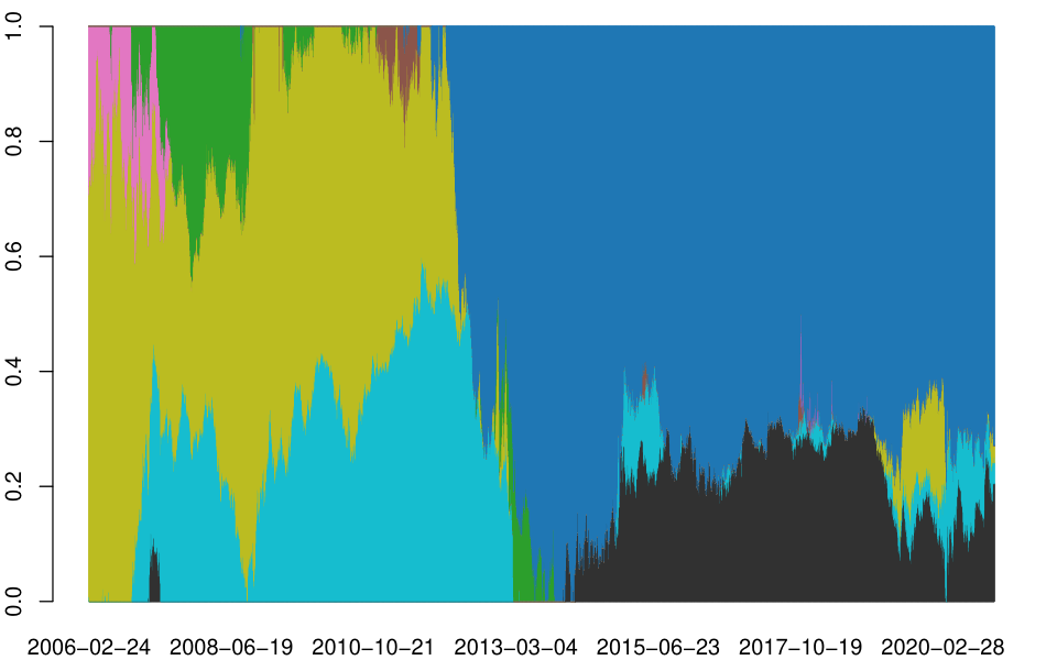
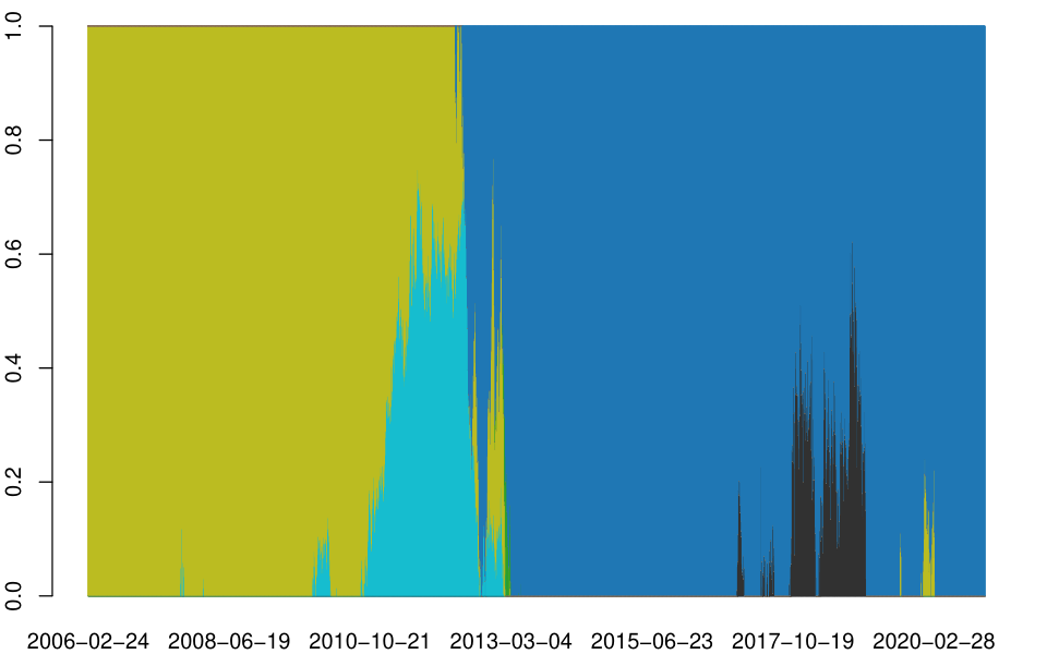
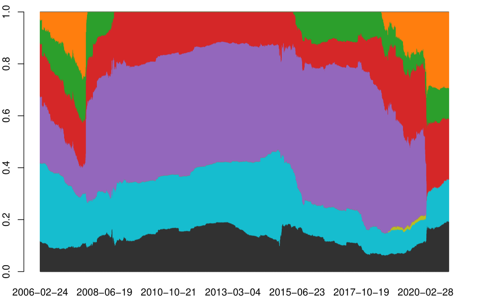
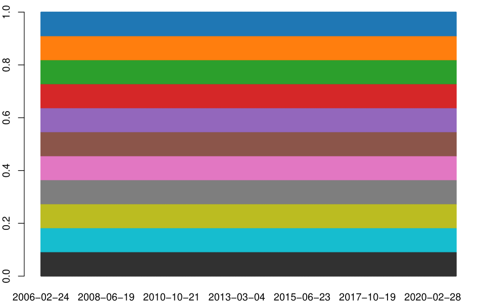
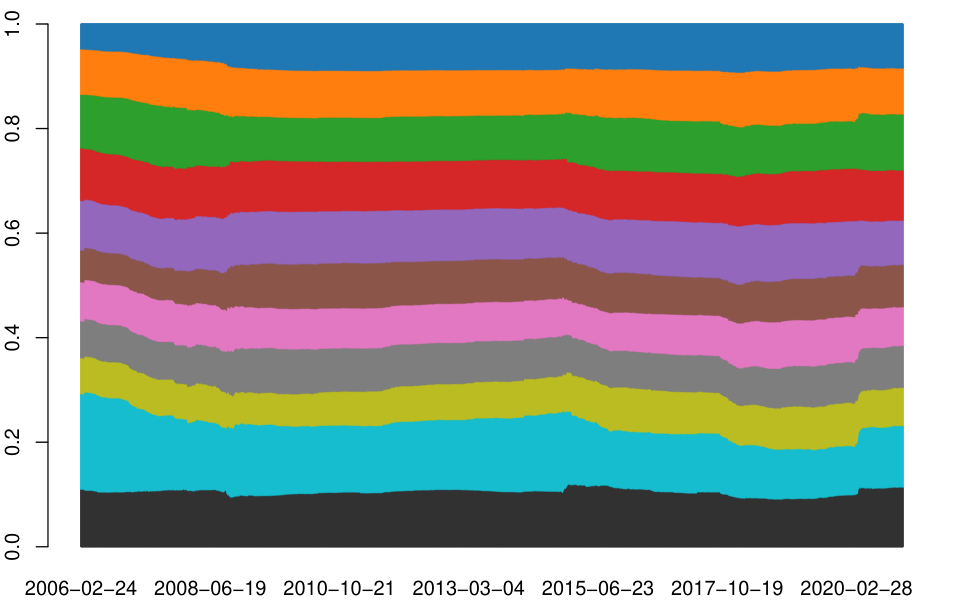
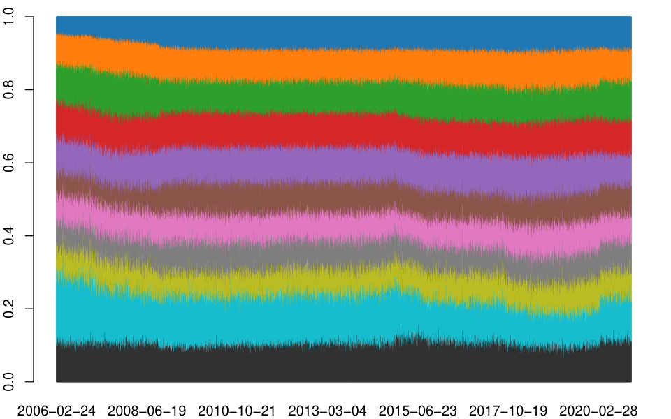
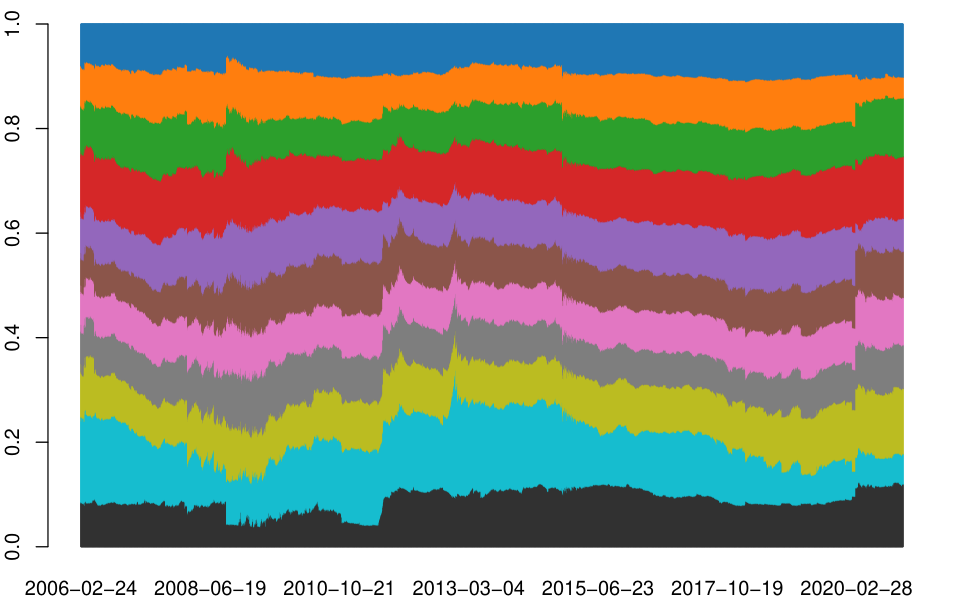
The weights of all 11 assets for each portfolio is presented in Figure 11. As suggested by Figure 9, msr, mmv, and gmv are the most dissimilar ones. From the weights of the mmv portfolio, we see that the mmv, for some periods of time, is fully invested in one single asset or, at most, two. A similar, although not so extreme, behaviour is observed for the msr and gmv portfolios. Both mmv and msr are strongly invested on NASDAQ 100 between 2013 and 2020. During this period, NASDAQ 100 presented extremely high returns, compared to the other assets in the sample, leading to similar behaviour in the portfolios.
Within the risk parity strategies, the first noticeable feature is the fact that all portfolios are much more balanced than msr, mmv, and gmv. Due to the nature of the assets under consideration (all with volatilities between 20% and 30%), the sdrp is, not surprisingly, similar to ew. As the empirical returns are sufficiently close to zero, the ES is proportional to the standard deviation under the Gaussian hypothesis (see Example 1). Therefore, the allocations under the grp95 should converge to those of sdrp when . This convergence is studied in Figure 12, where we present the grp95 portfolio generated using , instead of (Figure 11) samples in Algorithm 1. As expected, the grp computed with larger sample size is closer to sdrp.
The portfolio weights under the DCC-GARCH models (rpa95 and rpb95) are very similar, while the weights under the DCC-GJR-GARCH specification (rpb) appear to be more robust. This suggests that a more flexible model may be needed to take full advantage of the risk parity strategy using ES. Overall, the major movements observed in the sdrp weights are similar to those of both risk parity portfolios. For example, all risk parity portfolios start with a large proportion of wealth invested in the SSE Composite Index and the weights in that asset in the portfolios decrease steadily until the global financial crisis in 2008, after which the weights start to increase again. Differently from the msr and the mmv, a major change in the weights of the rpa95 and rpb95 portfolios is observed during the Covid-19 Pandemic.
It must be stressed that the behaviour of the risk parity portfolios constructed using the ES as a risk measure and complex multivariate dynamics for the returns is only currently possible due to the algorithms developed in this paper (Section 3).
7 Conclusions
We presented three optimisation algorithms tailored to the problem of constructing risk budgeting portfolios for coherent risk measures. One key benefits of the proposed algorithms is the fact that no analytical expressions for the densities of the assets’ returns is needed, indeed both our cutting planes algorithms and stochastic gradient descent algorithms rely only on scenarios of returns. We compare our cutting planes algorithm with standard convex optimisation solvers and show that our algorithm is significantly faster, particularly for increasing asset dimension and number of scenarios. Moreover, for a distortion risk measures with continuous distortion function and the Entropic VaR, only our cutting planes algorithm converges.
We apply our proposed algorithm to construct portfolios based on 11 equity indices and analyse the performance of the risk parity portfolios compared to other investment strategies. In this particular application we see that some of the risk parity portfolios are empirically similar to a portfolio with equal weights; a conclusion to date only available for risk parity portfolios using the standard deviation as a risk measure.
Acknowledgements
SP would like to acknowledge support from the Natural Sciences and Engineering Research Council of Canada (grants DGECR-2020-00333, RGPIN-2020-04289).
References
- Ahmadi-Javid, (2012) Ahmadi-Javid, A. (2012). Entropic value-at-risk: A new coherent risk measure. Journal of Optimization Theory and Applications, 155:1105–1123.
- Anis and Kwon, (2022) Anis, H. T. and Kwon, R. H. (2022). Cardinality-constrained risk parity portfolios. European Journal of Operational Research, 302(1):392–402.
- Artzner et al., (1999) Artzner, P., Delbaen, F., Eber, J.-M., and Heath, D. (1999). Coherent measures of risk. Mathematical Finance, 9(3):203–228.
- Bai et al., (2016) Bai, X., Scheinberg, K., and Tutuncu, R. (2016). Least-squares approach to risk parity in portfolio selection. Quantitative Finance, 16(3):357–376.
- Bellini et al., (2021) Bellini, F., Cesarone, F., Colombo, C., and Tardella, F. (2021). Risk parity with expectiles. European Journal of Operational Research, 291(3):1149–1163.
- Bollerslev, (1986) Bollerslev, T. (1986). Generalized autoregressive conditional heteroskedasticity. Journal of Econometrics, 31(3):307–327.
- Boudt et al., (2013) Boudt, K., Carl, P., and Peterson, B. G. (2013). Asset allocation with conditional Value-at-Risk budgets. Journal of Risk, 15(3):39–68.
- Bruder and Roncalli, (2012) Bruder, B. and Roncalli, T. (2012). Managing risk exposures using the risk budgeting approach. Available at SSRN 2009778.
- Cesarone and Tardella, (2017) Cesarone, F. and Tardella, F. (2017). Equal risk bounding is better than risk parity for portfolio selection. Journal of Global Optimization, 68(2):439–461.
- Chaves et al., (2012) Chaves, D., Hsu, J., Li, F., and Shakernia, O. (2012). Efficient algorithms for computing riskparity portfolio weights. The Journal of Investing, 21(3):150–163.
- Christoffersen et al., (1998) Christoffersen, P., Diebold, F. X., and Schuermann, T. (1998). Horizon problems and extreme events in financial risk management. Economic Policy Review, 4(3):98–16.
- da Costa, (2023) da Costa, B. F. P. (2023). RiskBudgeting: a package for risk budgeting portfolios. https://github.com/bfpc/RiskBudgeting.jl.
- Darolles et al., (2015) Darolles, S., Gourieroux, C., and Jay, E. (2015). Robust portfolio allocation with systematic risk contribution restrictions. In Risk-based and Factor Investing, pages 123–146. Elsevier.
- de M. Cardoso and Palomar, (2021) de M. Cardoso, J. V. and Palomar, D. P. (2021). riskParityPortfolio: Design of Risk Parity Portfolios. R package version 0.2.2.
- Dentcheva et al., (2010) Dentcheva, D., Penev, S., and Ruszczyński, A. (2010). Kusuoka representation of higher order dual risk measures. Annals of Operations Research, 181(1):325–335.
- Dhaene et al., (2012) Dhaene, J., Kukush, A., Linders, D., and Tang, Q. (2012). Remarks on quantiles and distortion risk measures. European Actuarial Journal, 2(2):319–328.
- Dunning et al., (2017) Dunning, I., Huchette, J., and Lubin, M. (2017). Jump: A modeling language for mathematical optimization. SIAM Review, 59(2):295–320.
- Engle, (2002) Engle, R. (2002). Dynamic conditional correlation: A simple class of multivariate generalized autoregressive conditional heteroskedasticity models. Journal of Business & Economic Statistics, 20(3):339–350.
- Feng and Palomar, (2015) Feng, Y. and Palomar, D. P. (2015). Scrip: Successive convex optimization methods for risk parity portfolio design. IEEE Transactions on Signal Processing, 63(19):5285–5300.
- Ghalanos, (2019) Ghalanos, A. (2019). rmgarch: Multivariate GARCH models. R package version 1.3-7.
- Glosten et al., (1993) Glosten, L. R., Jagannathan, R., and Runkle, D. E. (1993). On the relation between the expected value and the volatility of the nominal excess return on stocks. The Journal of Finance, 48(5):1779–1801.
- Grechuk, (2023) Grechuk, B. (2023). Extended gradient of convex function and capital allocation. European Journal of Operational Research, 305(1):429–437.
- Griveau-Billion et al., (2013) Griveau-Billion, T., Richard, J.-C., and Roncalli, T. (2013). A fast algorithm for computing high-dimensional risk parity portfolios. Available at SSRN 2325255.
- Hong and Liu, (2009) Hong, L. J. and Liu, G. (2009). Simulating sensitivities of conditional value at risk. Management Science, 55(2):281–293.
- Jurczenko and Teiletche, (2019) Jurczenko, E. and Teiletche, J. (2019). Expected shortfall asset allocation: A multi-dimensional risk-budgeting framework. The Journal of Alternative Investments, 22(2):7–22.
- Krokhmal, (2007) Krokhmal, P. A. (2007). Higher moment coherent risk measures. Quantitative Finance, 7:373–387.
- Ledoit and Wolf, (2017) Ledoit, O. and Wolf, M. (2017). Numerical implementation of the quest function. Computational Statistics & Data Analysis, 115:199–223.
- Li et al., (2021) Li, X., Uysal, A. S., and Mulvey, J. M. (2021). Multi-period portfolio optimization using model predictive control with mean-variance and risk parity frameworks. European Journal of Operational Research.
- Maillard et al., (2010) Maillard, S., Roncalli, T., and Teïletche, J. (2010). The properties of equally weighted risk contribution portfolios. The Journal of Portfolio Management, 36(4):60–70.
- Markowitz, (1952) Markowitz, H. (1952). Portfolio selection. Journal of Finance, 7(1):77–91.
- Mausser and Romanko, (2018) Mausser, H. and Romanko, O. (2018). Long-only equal risk contribution portfolios for CVaR under discrete distributions. Quantitative Finance, 18(11):1927–1945.
- Meyer and Quell, (2020) Meyer, C. and Quell, P. (2020). Risk Model Validation. Risk books.
- Mosek, (2022) Mosek (2022). Mosek.jl: Interface to the mosek solver in julia. https://github.com/MOSEK/Mosek.jl.
- O’Donoghue et al., (2016) O’Donoghue, B., Chu, E., Parikh, N., and Boyd, S. (2016). Conic optimization via operator splitting and homogeneous self-dual embedding. Journal of Optimization Theory and Applications, 169(3):1042–1068.
- Perlin, (2020) Perlin, M. (2020). BatchGetSymbols: Downloads and Organizes Financial Data for Multiple Tickers. R package version 2.6.1.
- Pesenti et al., (2021) Pesenti, S. M., Millossovich, P., and Tsanakas, A. (2021). Cascade sensitivity measures. Risk Analysis, 41:2392–2414.
- Prékopa, (1995) Prékopa, A. (1995). Stochastic programming, volume 324. Kluwer Academic Publishers.
- Qian, (2005) Qian, E. (2005). Risk parity portfolios: Efficient portfolios through true diversification. Panagora Asset Management.
- Ramprasad, (2016) Ramprasad, P. (2016). nlshrink: Non-Linear Shrinkage Estimation of Population Eigenvalues and Covariance Matrices. R package version 1.0.1.
- Rockafellar and Uryasev, (2000) Rockafellar, R. T. and Uryasev, S. (2000). Optimization of conditional Value-at-Risk. Journal of Risk, 2:21–42.
- Roncalli, (2013) Roncalli, T. (2013). Introduction to risk parity and budgeting. CRC Press.
- Shapiro et al., (2009) Shapiro, A., Dentcheva, D., and Ruszczyński, A. (2009). Lectures on stochastic programming: modeling and theory. SIAM.
- Sharpe, (1966) Sharpe, W. F. (1966). Mutual fund performance. The Journal of Business, 39(1):119–138.
- Spinu, (2013) Spinu, F. (2013). An algorithm for computing risk parity weights. Available at SSRN 2297383.
- Tasche, (1999) Tasche, D. (1999). Risk contributions and performance measurement. Report of the Lehrstuhl für mathematische Statistik, TU München.
- Tsanakas, (2009) Tsanakas, A. (2009). To split or not to split: Capital allocation with convex risk measures. Insurance: Mathematics and Economics, 44(2):268–277.
- Tsanakas and Millossovich, (2016) Tsanakas, A. and Millossovich, P. (2016). Sensitivity analysis using risk measures. Risk Analysis, 36(1):30–48.
- Udell et al., (2014) Udell, M., Mohan, K., Zeng, D., Hong, J., Diamond, S., and Boyd, S. (2014). Convex optimization in Julia. SC14 Workshop on High Performance Technical Computing in Dynamic Languages.
- Wächter and Biegler, (2006) Wächter, A. and Biegler, L. T. (2006). On the implementation of a primal-dual interior point filter line search algorithm for large-scale nonlinear programming. Mathematical Programming, 106:25–57.
Appendix A Numerical studies
In this section we provide additional plots for the numerical exercises of Section 4. Figures 13 and 14 complement, respectively, the multivariate Gaussian and Student analysis for the ES with and . Figures 15 and 6 show the run times for the multivariate Student for the Entropic VaR and distortion risk measures, respectively.
Appendix B Summary statistics
Table 5 reports the annualised volatility, annualised return, and annual Sharpe ratio, as well as the , , and the maximum drawdown of all considered portfolios. We observe that the statistics for the risk parity portfolios with different ES security level do not change drastically.
| Volatility | Return | Sharpe | Max drawdown | |||
| sdrp | 18.44% | 9.37% | 0.508 | -1.67% | -2.91% | -59.89% |
| msr | 23.54% | 12.88% | 0.547 | -2.05% | -3.67% | -70.75% |
| gmv | 17.02% | 9.71% | 0.571 | -1.56% | -2.69% | -58.36% |
| mmv | 26.87% | 14.79% | 0.551 | -2.56% | -4.21% | -66.58% |
| ew | 18.89% | 8.80% | 0.466 | -1.69% | -2.97% | -59.48% |
| grp80 | 18.49% | 9.40% | 0.508 | -1.70% | -2.91% | -60.74% |
| grp85 | 18.49% | 9.38% | 0.507 | -1.70% | -2.91% | -60.62% |
| grp90 | 18.50% | 9.49% | 0.513 | -1.71% | -2.91% | -60.38% |
| grp95 | 18.51% | 9.58% | 0.517 | -1.69% | -2.91% | -60.36% |
| grp96 | 18.53% | 9.45% | 0.510 | -1.69% | -2.92% | -60.32% |
| grp97 | 18.52% | 9.33% | 0.504 | -1.70% | -2.92% | -60.24% |
| grp98 | 18.53% | 9.23% | 0.498 | -1.69% | -2.92% | -60.23% |
| grp99 | 18.56% | 9.43% | 0.508 | -1.69% | -2.92% | -59.99% |
| rpa80 | 18.89% | 8.89% | 0.471 | -1.69% | -2.99% | -60.26% |
| rpa85 | 18.82% | 8.90% | 0.473 | -1.68% | -2.98% | -60.40% |
| rpa90 | 18.79% | 8.93% | 0.475 | -1.68% | -2.97% | -60.34% |
| rpa95 | 18.88% | 8.93% | 0.473 | -1.69% | -2.99% | -60.22% |
| rpa96 | 18.96% | 9.04% | 0.477 | -1.70% | -3.00% | -60.19% |
| rpa97 | 19.02% | 9.03% | 0.475 | -1.72% | -3.01% | -60.28% |
| rpa98 | 19.13% | 8.98% | 0.469 | -1.72% | -3.02% | -59.89% |
| rpa99 | 19.33% | 8.87% | 0.459 | -1.70% | -3.06% | -59.83% |
| rpb80 | 18.89% | 8.89% | 0.471 | -1.68% | -2.99% | -60.34% |
| rpb85 | 18.83% | 8.85% | 0.470 | -1.67% | -2.98% | -60.27% |
| rpb90 | 18.76% | 8.90% | 0.474 | -1.66% | -2.97% | -60.37% |
| rpb95 | 18.71% | 8.78% | 0.469 | -1.66% | -2.96% | -60.25% |
| rpb96 | 18.75% | 8.77% | 0.468 | -1.66% | -2.97% | -60.28% |
| rpb97 | 18.75% | 8.93% | 0.476 | -1.68% | -2.96% | -60.19% |
| rpb98 | 18.77% | 9.00% | 0.479 | -1.67% | -2.97% | -60.21% |
| rpb99 | 18.76% | 8.90% | 0.474 | -1.66% | -2.96% | -59.69% |