De Novo Molecular Generation via
Connection-aware Motif Mining
Abstract
De novo molecular generation is an essential task for science discovery. Recently, fragment-based deep generative models have attracted much research attention due to their flexibility in generating novel molecules based on existing molecule fragments. However, the motif vocabulary, i.e., the collection of frequent fragments, is usually built upon heuristic rules, which brings difficulties to capturing common substructures from large amounts of molecules. In this work, we propose a new method, MiCaM, to generate molecules based on mined connection-aware motifs. Specifically, it leverages a data-driven algorithm to automatically discover motifs from a molecule library by iteratively merging subgraphs based on their frequency. The obtained motif vocabulary consists of not only molecular motifs (i.e., the frequent fragments), but also their connection information, indicating how the motifs are connected with each other. Based on the mined connection-aware motifs, MiCaM builds a connection-aware generator, which simultaneously picks up motifs and determines how they are connected. We test our method on distribution-learning benchmarks (i.e., generating novel molecules to resemble the distribution of a given training set) and goal-directed benchmarks (i.e., generating molecules with target properties), and achieve significant improvements over previous fragment-based baselines. Furthermore, we demonstrate that our method can effectively mine domain-specific motifs for different tasks.
1 Introduction
Drug discovery, from designing hit compounds to developing an approved product, often takes more than ten years and billions of dollars (Hughes et al. 2011). De novo molecular generation is a fundamental task in drug discovery, as it provides novel drug candidates and determines the underlying quality of final products. Recently, with the development of artificial intelligence, deep neural networks, especially graph neural networks (GNNs), have been widely used to accelerate novel molecular generation (Stokes et al. 2020; Bilodeau et al. 2022). Specifically, we can employ a GNN to generate a molecule iteratively: in each step, given an unfinished molecule , we first determine a new generation unit to be added; next, determine the connecting sites on and ; and finally determine the attachments between the connecting sites, e.g., creating new bonds (Liu et al. 2018) or merging shared atoms (Jin et al. 2018). In different methods, the generation units could be either atoms (Li et al. 2018; Mercado et al. 2021) or frequent fragments (referred to as motifs) (Jin et al. 2020a; Kong et al. 2021; Maziarz et al. 2021).
For fragment-based models, building an effective motif vocabulary is a key factor to the success of molecular generation (Maziarz et al. 2021). Previous works usually rely on heuristic rules or templates to obtain a motif vocabulary. For example, JT-VAE (Jin et al. 2018) decomposes molecules into pre-defined structures like rings, chemical bonds, and individual atoms, while MoLeR (Maziarz et al. 2021) separates molecules into ring systems and acyclic linkers or functional groups. Several other works build motif vocabularies in a similar manner (Jin et al. 2020a; Yang et al. 2021). However, heuristic rules cannot cover some chemical structures that commonly occur yet are a bit more complex than pre-defined structures. For example, the subgraph patterns benzaldehyde (“O=Cc1ccccc1”) and trifluoromethylbenzene (“FC(F)(F)c1ccccc1”) (as shown in Figure 1) occur 398,760 times and 57,545 times respectively in the 1.8 million molecules in ChEMBL (Mendez et al. 2019), and both of them are industrially useful. Despite their high frequency in molecules, the aforementioned methods cannot cover such common motifs. Moreover, in different concrete generation tasks, different motifs with some domain-specific structures or patterns are favorable, which can hardly be enumerated by existing rules. Another important factor that affects the generation quality is the connection information of motifs. This is because although many connections are valid under a valence check, the “reasonable” connections are predetermined and reflected by the data distribution, which contribute to the chemical properties of molecules (Yang et al. 2021). For example, a sulfur atom with two triple-bonds, i.e., “*#S#*” (see Figure 1), is valid under a valence check but is “unreasonable” from a chemical point of view and does not occur in ChEMBL.


In this work, we propose MiCaM, a generative model based on Mined Connection-aware Motifs. It includes a data-driven algorithm to mine a connection-aware motif vocabulary from a molecule library, as well as a connection-aware generator for de novo molecular generation. The algorithm mines the most common substructures based on their frequency of appearance in the molecule library. Briefly, across all molecules in the library, we find the most frequent fragment pairs that are adjacent in graphs, and merge them into an entire fragment. We repeat this process for a pre-defined number of steps and collect the fragments to build a motif vocabulary. We preserve the connection information of the obtained motifs, and thus we call them connection-aware motifs.
Based on the mined vocabulary, we design the generator to simultaneously pick up motifs to be added and determine the connection mode of the motifs. In each generation step, we focus on a non-terminal connection site in the current generated molecule, and use it to query another connection either (1) from the motif vocabulary, which implies connecting a new motif, or (2) from the current molecule, which implies cyclizing the current molecule.
We evaluate MiCaM on distribution learning benchmarks from GuacaMol (Brown et al. 2019), which aim to resemble the distributions of given molecular sets. We conduct experiments on three different datasets and MiCaM achieves the best overall performance compared with several strong baselines. After that, we also work on goal directed benchmarks, which aim to generate molecules with specific target properties. We combine MiCaM with iterative target augmentation (Yang et al. 2020) by jointly adapting the motif vocabulary and network parameters. In this way, we achieve state-of-the-art results on four different types of goal-directed tasks, and find motif patterns that are relevant to the target properties.
2 Our Approach
2.1 Connection-aware Molecular Motif Mining

Our motif mining algorithm aims to find the common molecule motifs from a given training data set , and build a connection-aware motif vocabulary for the follow-up molecular generation. It processes with two phases: the merging-operation learning phase and the motif-vocabulary construction phase. Figure 2 presents an example and more implementation details are in Algorithm 1 in Appendix A.1.
Merging-operation Learning Phase
In this phase, we aim to learn the top most common patterns (which correspond to rules indicating how to merge subgraphs) from the training data , where is a hyperparameter. Each molecule in is represented as a graph (the first row in Figure 2(a)), where the nodes and edges denote atoms and bonds respectively. For each , we use a merging graph (the second row in Figure 2(a)) to track the merging status, i.e., to represent the fragments and their connections. In , each node represents a fragment (either an atom or a subgraph) of the molecule, and the edges in indicate whether two fragments are connected with each other. We initialize each merging graph from the molecule graph by treating each atom as a single fragment and inheriting the bond connections from , i.e., .
We define an operation “” to create a new fragment by merging two fragments and together. The newly obtained contains all nodes and edges from , , as well as all edges between them. We iteratively update the merging graphs to learn merging operations. In the merging graph at the iteration (), each edge represents a pair of fragments, , that are adjacent in the molecule. It also gives out a new fragment . We traverse all edges in all merging graphs to count the frequency of , and denote the most frequent as . 11 1 Different can make same . For example, both and can make “CCCC”. Consequently, the -th merging operation is defined as: if , then merge and together.22 2 When applying merging operations, we traverse edges in orders given by RDKit (Landrum et al. 2006). We apply the merging operation on all merging graphs to update them into . We repeat such a process for iterations to obtain a merging operation sequence .
Motif-vocabulary Construction Phase
For each molecule , we apply the merging operations sequentially to obtain the ultimate merging graph . We then disconnect all edges between different fragments and add the symbols “” to the disconnected positions (see Figure 2(b, c)). The fragments with “” symbols are connection-aware, and we denote the connection-aware version of a fragment as . The motif vocabulary is the collection of all such connection-aware motifs: . During generating, our model connects the motifs together by directly merging the connection sites (i.e., the “”s) to generate new molecules.
Time Complexity
The time complexity of learning merging operations is , where is the number of iterations, is the molecule library size, and . In practice, the time cost decreases rapidly as the iteration step increases. It takes less than minutes and about minutes to run iterations on the QM9 ( molecules) (Ruddigkeit et al. 2012) and ZINC ( molecules) (Irwin et al. 2012) datasets, respectively, using CPU cores (see Appendix A.1). The time complexity of fragmentizing an arbitrary molecule into motifs is , linear with the number of bonds.
2.2 Molecular Generation with Connection-aware Motifs
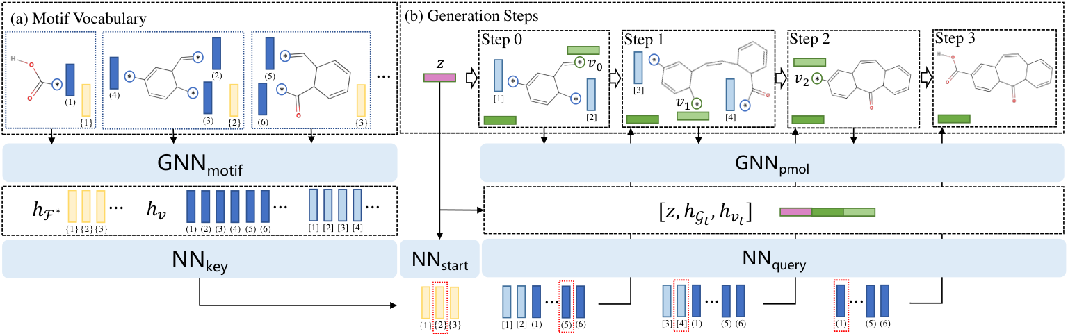
The generation procedure of MiCaM is shown in Figure 3 and Algorithm 2 in Appendix A.2. MiCaM generates molecules by gradually adding new motifs to a current partial molecule (denoted as , where is the generation step), or merging two connection sites in to form a new ring.
For ease of reference, we define the following notations. We denote the node representation of any atom (including the connection sites) as , and denote the graph representation of any graph (either a molecule or a motif) as . Let denote the connection sites from a graph (either a partial molecule or a motif), and let be the set of all connection sites from the motif vocabulary.
Generation Steps
In the generation step, MiCaM modifies the partial molecule as follows:
(1) Focus on a connection site from . We use a queue to manage the the orders of connection sites in . At the step, we pop the head of to get a connection site . The is maintained as follows: after selecting a new motif to connect with , we use the RDKit library to give a canonical order of the atoms in , and then put the connection sites into following this order. After merging two connection sites together, we just remove them from .
(2) Encode and candidate connections. We employ a graph neural network GNN to encode the partial molecule and obtain the representations of all atoms (including the connection sites) and the graph. The node representations of and the graph representation of will be jointly used to query another connection site. For the motifs , we use another GNN, denoted as GNN, to encode their atoms and connection sites. In this way we obtain the node representations of all connection sites 33 3 During inference, the motif representations can be calculated offline to avoid additional computation time.. The candidate connections are either from or from .
(3) Query another connection site. We employ two neural networks, NN to make a query vector, and NN to make key vectors, respectively. Specifically, the probability of picking every connection sites is calculated by:
| (1) |
where is a latent vector as used in variational auto-encoder (VAE) (Kingma & Welling 2013). Using different results in diverse molecules. During training, is sampled from a posterior distribution given by an encoder, while during inference, is sampled from a prior distribution.
For inference, we make a constraint on the bond type of picked by only considering the connection sites whose adjacent edges have the same bond type as . This practice guarantees the validity of the generated molecules. We also implement two generation modes, i.e., greedy mode that picks the connection as , and distributional mode that samples the connection from .
(4) Connect a new motif or cyclize. After the model picks a connection , it turns into a connecting phase or a cyclizing phase, depending on whether or . If , and suppose that , then we connect with by directly merging and . Otherwise, when , we merge and together to form a new ring, and thus the molecule cyclizes itself. Notice that, allowing the picked connection site to come from the partial molecule is important, because with this mechanism MiCaM theoretically can generate novel rings that are not in the motif vocabulary.
We repeat these steps until is empty and thus there is no non-terminal connection site in the partial molecule, which indicates that we have generated an entire molecule.
Starting
As in the beginning (i.e., the step), the partial graph is empty, we implement this step exceptionally. Specifically, we use another neural network NN to pick up the first motif from the vocabulary as . The probability of picking every motifs is calculated by:
| (2) |
2.3 Training MiCaM
We train our model in a VAE (Kingma & Welling 2013) paradigm.44 4 MiCaM can be naturally paired with other paradigms such as GAN or RL, which we plan to explore in future works. A standard VAE has an encoder and a decoder. The encoder maps the input molecule to its representation , and then builds a posterior distribution of the latent vector based on . The decoder takes as input and tries to reconstruct the . VAE usually has a reconstruction loss term (between the original input and the reconstructed ) and a regularization term (to control the posterior distribution of ).
In our work, we use a GNN model GNN as the encoder to encode a molecule and obtain its representation . The latent vecotr is then sampled from a posterior distribution , where and output the mean and log variance, respectively. How to use is explained in Equation (1) and (2). The decoder consists of GNN, GNN, NN, NN and NN that jointly work to generate molecules.
The overall training objective function is defined as:
| (3) |
In Equation (3): (1) is the reconstruction loss as that in a standard VAE. It uses cross entropy loss to evaluate the likelihood of the reconstructed graph compared with the input . (2) The loss is used to regularize the posterior distribution in the latent space. (3) Following Maziarz et al. 2021, we add a property prediction loss to ensure the continuity of the latent space with respect to some simple molecule properties. Specifically, we build another network NNprop to predict the properties from the latent vector . (4) and are hyperparameters to be determined according to validation performances.
Here we emphasize two useful details. (1) Since MiCaM is an iterative method, in the training procedure, we need to determine the orders of motifs to be processed. The orders of the intermediate motifs (i.e., ) are determined by the queue introduced in Section 2.2. The only remaining item is the first motif, and we choose the motif with the largest number of atoms as the first one. The intuition is that the largest motif mostly reflects the molecule’s properties. The generation order is then determined according to Algorithm 2. (2) In the training procedure, we provide supervisions for every individual generation steps. We implement the reconstruction loss by viewing the generation steps as parallel classification tasks. In practice, as the vocabulary size is large due to various possible connections, is costly to compute. To tackle this problem, we subsample the vocabulary and modify via contrastive learning (He et al. 2020). More details can be found in Appendix A.4.
2.4 Discussion and Related Work
Molecular Generation
A plethora of existing generative models are available and they fall into two categories: (1) string-based models (Kusner et al. 2017; Gómez-Bombarelli et al. 2018; Sanchez-Lengeling & Aspuru-Guzik 2018; Segler et al. 2018), which rely on string representations of molecules such as SMILES (Weininger 1988) and do not utilize the structual information of molecules, (2) and graph-based models (Liu et al. 2018; Guo et al. 2021) that are naturally based on molecule graphs. Graph-based approaches mainly include models that generate molecular graphs (1) atom-by-atom (Li et al. 2018; Mercado et al. 2021), and (2) fragment-by-fragment (Kong et al. 2021; Maziarz et al. 2021; Zhang et al. 2021; Guo et al. 2021). This work is mainly related to fragment-based methods.
Motif Mining
Our motif mining algorithm is inspired by Byte Pair Encoding (BPE) (Gage 1994), which is widely adapted in natural language processing (NLP) to tokenize words into subwords (Sennrich et al. 2015). Compared with BPE in NLP, molecules have much more complex structures due to different connections and bond types, which we solve by building the merging graphs. Another related class of algorithms are Frequent Subgraph Mining (FSM) algorithms (Kuramochi & Karypis 2001; Jiang et al. 2013), which also aim to mine frequent motifs from graphs. However, these algorithms do not provide a “tokenizer” to fragmentize an arbitrary molecule into disjoint fragments, like what is done by BPE. Thus we cannot directly apply them in molecular generation tasks. Kong et al. 2021 also try to mine motifs, but they do not incorporate the connection information into the motif vocabulary and they apply a totally different generation procedure, which are important to the performance (see Appendix B.3). See Appendix D for more discussions.
Motif Representation
Different from many prior works that view motifs as discrete tokens, we represent all the motifs in the motif vocabulary as graphs, and we apply the GNN to obtain the representations of motifs. This novel approach has three advantages. (1) The GNN obtains similar representations for similar motifs, which thus maintains the graph structure information of the motifs (see Appendix C.3). (2) The GNN, combined with contrastive learning, can handle large size of motif vocabulary in training, which allows us to construct a large motif vocabulary (see Section 2.3 and Apppendix A.4). (3) The model can be easily transferred to another motif vocabulary. Thus we can jointly tune the motif vocabulary and the network parameters on a new dataset, improving the capability of the model to fit new data (see Section 3.2).
3 Experiments
3.1 Distributional Learning Results
To demonstrate the effectiveness of MiCaM, we test it on the benchmarks from GuacaMol (Brown et al. 2019), a commonly used evaluation framework to assess de novo molecular generation models.55 5 The code of MiCaM is available at https://github.com/MIRALab-USTC/AI4Sci-MiCaM. We first consider the distribution learning benchmarks, which assess how well the models learn to generate novel molecules that resemble the distribution of the training set.
Experimental Setup
Following Brown et al. 2019, we consider five metrics for distribution learning: validity, uniqueness, novelty, KL divergence (KL Div) and Fréchet ChemNet Distance (FCD). The first three metrics measure if the model can generate chemically valid, unique, and novel candidate molecules, while last two are designed to measure the distributional similarity between the generated molecules and the training set. For the KL Div benchmark, we compare the probability distributions of a variety physicochemial descriptors. A higher KL Div score, i.e., lower KL divergences for the descriptors, means that the generated molecules resemble the training set in terms of these descriptors. The FCD is calculated from the hidden representations of molecules in a neural network called ChemNet (Preuer et al. 2018), which can capture important chemiacal and biological features of molecules. A higher FCD score, i.e., a lower Fréchet ChemNet Distance means that the generated molecules have similar chemical and biological properties to those from the training set.
We evaluate our method on three datasets: QM9 (Ruddigkeit et al. 2012), ZINC (Irwin et al. 2012), and GuacaMol (a post-processed ChEMBL (Mendez et al. 2019) dataset proposed by Brown et al. 2019). These three datasets cover different molecule complexities and different data sizes. The results across them demonstrate the capability of our model to handle different kinds of data.
Quantitative Results
| Dadaset | Model | Validity | Uniqueness | Novelty | KL Div | FCD |
| QM9 | JT-VAE | 1.0 | 0.549 | 0.386 | 0.891 | 0.588 |
| GCPN | 1.0 | 0.533 | 0.320 | 0.552 | 0.174 | |
| GP-VAE | 1.0 | 0.673 | 0.523 | 0.921 | 0.659 | |
| MoLeR | 1.0 | 0.940 | 0.355 | 0.969 | 0.931 | |
| MiCaM (Ours) | 1.0 | 0.932 | 0.493 | 0.980 | 0.945 | |
| ZINC | JT-VAE | 1.0 | 0.988 | 0.988 | 0.882 | 0.263 |
| GCPN | 1.0 | 0.982 | 0.982 | 0.456 | 0.003 | |
| GP-VAE | 1.0 | 0.997 | 0.997 | 0.850 | 0.318 | |
| MoLeR | 1.0 | 0.996 | 0.993 | 0.984 | 0.721 | |
| MiCaM (Ours) | 1.0 | 0.998 | 0.997 | 0.988 | 0.791 | |
| GuacaMol | MoLeR | 1.0 | 1.000 | 0.991 | 0.964 | 0.625 |
| MiCaM (Ours) | 1.0 | 0.994 | 0.986 | 0.989 | 0.731 |
Table 1 presents our experimental results of distribution learning tasks. We compare our model with several state-of-the-art models: JT-VAE (Jin et al. 2018), GCPN (You et al. 2018), GP-VAE (Kong et al. 2021), and MoLeR (Maziarz et al. 2021). Since all the models are graph-based, they obtain validity by introducing chemical valence check during generation. We can see that MiCaM achieves the best performances on the KL Divergence and FCD scores on all the three datasets, which demonstrates that it can well resemble the distributions of training sets. Meanwhile it keeps high uniqueness and novelty, comparable to previous best results. In this experiment, we set the number of merging operations to be for QM9, due to the results in Figure 4. For ZINC and GuacaMol, we simply set the number to be and find that MiCaM has achieved performances that outperform all the baselines. This indicates that existing methods tend to perform well on the sets of relatively simple molecules such as QM9, while MiCaM performs well on datasets with variant complexity. We further visualize the distributions in Figure 7 of Appendix B.2.
Number of Merging Operations
We conduct experiments on different choices of the number of merging operations. Figure 4 presents the experimental results on QM9. It shows that FCD score and KL Divergence score, which measure the similarity between the generated molecules and the training set, increase as the number of merging operations grows. Meanwhile, the novelty decreases as the number grows. Intuitively, the more merging operations we use for motif vocabulary construction, the larger motifs will be contained in the vocabulary, and thus will induce more structural information from the training set. We can achieve a trade-off between the similarity and novelty by controlling the number of merging operations. Empirically, a medium number (about ) of operations is enough to achieve a high similarity.
Generation Modes
We also compare two different generation modes, i.e., the greedy mode and the distributional mode. With the greedy mode, the model always picks the motif or the connection site with the highest probability. While the distributional mode allows picking motifs or connection sites according to a distribution. The results show that the greedy mode leads to a little higher KL Divergence and FCD scores, while the distributional mode leads to a higher novelty.
3.2 Goal Directed Generation Results
| Benchmark | Dataset |
|
|
|
|
MSO |
| ||||||||||
|---|---|---|---|---|---|---|---|---|---|---|---|---|---|---|---|---|---|
| a. | 0.505 | 0.732 | 0.355 | 1.000 | 1.000 | 1.000 | 1.000 | ||||||||||
| b. | 0.595 | 0.834 | 0.380 | 1.000 | 1.000 | 1.000 | 1.000 | ||||||||||
| c. | 0.684 | 0.829 | 0.410 | 0.971 | 0.993 | 0.997 | 0.999 | ||||||||||
| d. | 0.792 | 0.881 | 0.616 | 0.920 | 0.855 | 0.931 | 0.932 | ||||||||||
| e. | 0.509 | 0.689 | 0.458 | 0.891 | 0.545 | 0.868 | 0.914 |
We further demonstrate the capability of our model to generate molecules with wanted properties. In such goal directed generation tasks, we aim to generate molecules that have high scores which are predefined by rules.
Iteratively Tuning
We combine MiCaM with iterative target augmentation (ITA) (Yang et al. 2020) and generate optimized molecules by iteratively generating new molecules and tuning the model on molecules with highest scores. Specifically, we first pick out molecules with top scores from the GuacaMol dataset and store them in a training buffer. Iteratively, we tune our model on the training buffer and generate new molecules. In each iteration, we update the training buffer to store the top molecules that are either newly generated or from the training buffer in the last iteration. In order to accelerate the model to explore the latent space, we pair MiCaM with Molecular Swarm Optimization (MSO) (Winter et al. 2019) in each iteration to generate new molecules.
A novelty of our approach is that when tuning on a new dataset, we jointly update the motif vocabulary and the network parameters. We can do this because we apply a GNN to obtain motif representations, which can be transferred to a newly built motif vocabulary. The representations of the new motifs are calculated by GNN, and we then optimize the network parameters using both new data and newly constructed motif vocabulary.
Experimental Setup
We test MiCaM on several goal directed generation tasks from GuacaMol benchmarks. Specifically, we consider four different categories of tasks: a Rediscovery task (Celecoxib Rediscovery), a Similarity task (Aripiprazole Similarity), an Isomers task ( Isomers), and two multi-property objective (MPO) tasks (Ranolazine MPO and Sitagliptin MPO). We compare MiCaM with several strong baselines.
Quantitative Results
For each benchmark, we run iterations. In each iteration, we apply MSO to generate molecules, and store molecules with highest scores in the training buffer to tune MiCaM. We tune the model pretrained on the GuacaMol dataset and Table 2 presents the results. MiCaM achieves scores on some relatively easy benchmarks. It achieves high scores on several difficult benchmarks such MPO tasks, outperforming the baselines.
Case Studies
There are some domain-specific motifs that are beneficial to the target properties in different goal directed generation tasks, which are likely to be the pharmacophores in drug molecules. We conduct case studies to demonstrate the ability of MiCaM to mine such favorable motifs for domain-specific tasks.
In Figure 5 we present cases for the Ranolazine MPO benchmark, which tries to discover molecules similar to Ranolazine, a known drug molecule, but with additional requirements on some other properties. This benchmark calculates the geometric mean of four scores: Sim (the similarity between the molecule and Ranolazine), logP, TPSA, and Num_Fs (the number of fluorine atoms). We present a generation trajectory as well as the scores in each generation step. Due to the domain-specific motif vocabulary and the connection query mechanism, it requires only a few steps to generate such a complex molecule. Moreover, we can see that the scores increase as some key motifs are added to the molecule, which implies that the picked motifs are relevant to the target properties. See Figure 8 in Appendix B.4 for more case studies.
4 Conclusion
In this work, we proposed MiCaM, a novel model that generates molecules based on mined connection-aware motifs. Specifically, the contributions include (1) a data-driven algorithm to mine motifs by iteratively merging most frequent subgraph patterns and (2) a connection-aware generator for de novo molecular generation. It achieve state-of-the-art results on distribution learning tasks and on three different datasets. Combined with iterative target augmentation, it can learn domain-specific motifs related to some properties and performs well on goal directed benchmarks.
Acknowledgement
The authors would like to thank all the anonymous reviewers for their insightful comments. This work was supported in part by National Nature Science Foundations of China grants U19B2026, U19B2044, 61836011, 62021001, and 61836006, and the Fundamental Research Funds for the Central Universities grant WK3490000004.
References
- Ahn et al. (2020) Sungsoo Ahn, Junsu Kim, Hankook Lee, and Jinwoo Shin. Guiding deep molecular optimization with genetic exploration. Advances in neural information processing systems, 33:12008–12021, 2020.
- Bilodeau et al. (2022) Camille Bilodeau, Wengong Jin, Tommi Jaakkola, Regina Barzilay, and Klavs F Jensen. Generative models for molecular discovery: Recent advances and challenges. Wiley Interdisciplinary Reviews: Computational Molecular Science, pp. e1608, 2022.
- Bowman et al. (2015) Samuel R Bowman, Luke Vilnis, Oriol Vinyals, Andrew M Dai, Rafal Jozefowicz, and Samy Bengio. Generating sentences from a continuous space. arXiv preprint arXiv:1511.06349, 2015.
- Brown et al. (2019) Nathan Brown, Marco Fiscato, Marwin HS Segler, and Alain C Vaucher. Guacamol: benchmarking models for de novo molecular design. Journal of chemical information and modeling, 59(3):1096–1108, 2019.
- Chen et al. (2021) Binghong Chen, Tianzhe Wang, Chengtao Li, Hanjun Dai, and Le Song. Molecule optimization by explainable evolution. In International Conference on Learning Representation (ICLR), 2021.
- Degen et al. (2008) Jörg Degen, Christof Wegscheid-Gerlach, Andrea Zaliani, and Matthias Rarey. On the art of compiling and using’drug-like’chemical fragment spaces. ChemMedChem: Chemistry Enabling Drug Discovery, 3(10):1503–1507, 2008.
- Fan (2021) Jiajun Fan. A review for deep reinforcement learning in atari: Benchmarks, challenges, and solutions. arXiv preprint arXiv:2112.04145, 2021.
- Fan & Xiao (2022) Jiajun Fan and Changnan Xiao. Generalized data distribution iteration. arXiv preprint arXiv:2206.03192, 2022.
- Gage (1994) Philip Gage. A new algorithm for data compression. C Users Journal, 12(2):23–38, 1994.
- Gómez-Bombarelli et al. (2018) Rafael Gómez-Bombarelli, Jennifer N Wei, David Duvenaud, José Miguel Hernández-Lobato, Benjamín Sánchez-Lengeling, Dennis Sheberla, Jorge Aguilera-Iparraguirre, Timothy D Hirzel, Ryan P Adams, and Alán Aspuru-Guzik. Automatic chemical design using a data-driven continuous representation of molecules. ACS central science, 4(2):268–276, 2018.
- Guo et al. (2021) Minghao Guo, Veronika Thost, Beichen Li, Payel Das, Jie Chen, and Wojciech Matusik. Data-efficient graph grammar learning for molecular generation. In International Conference on Learning Representations, 2021.
- He et al. (2022) Hua-Rui He, Jie Wang, Yunfei Liu, and Feng Wu. Modeling diverse chemical reactions for single-step retrosynthesis via discrete latent variables. In Proceedings of the 31st ACM International Conference on Information & Knowledge Management, pp. 717–726, 2022.
- He et al. (2020) Kaiming He, Haoqi Fan, Yuxin Wu, Saining Xie, and Ross Girshick. Momentum contrast for unsupervised visual representation learning. In Proceedings of the IEEE/CVF conference on computer vision and pattern recognition, pp. 9729–9738, 2020.
- Hu et al. (2019) Weihua Hu, Bowen Liu, Joseph Gomes, Marinka Zitnik, Percy Liang, Vijay Pande, and Jure Leskovec. Strategies for pre-training graph neural networks. arXiv preprint arXiv:1905.12265, 2019.
- Hughes et al. (2011) James P Hughes, Stephen Rees, S Barrett Kalindjian, and Karen L Philpott. Principles of early drug discovery. British journal of pharmacology, 162(6):1239–1249, 2011.
- Irwin et al. (2012) John J Irwin, Teague Sterling, Michael M Mysinger, Erin S Bolstad, and Ryan G Coleman. Zinc: a free tool to discover chemistry for biology. Journal of chemical information and modeling, 52(7):1757–1768, 2012.
- Jensen (2019) Jan H Jensen. A graph-based genetic algorithm and generative model/monte carlo tree search for the exploration of chemical space. Chemical science, 10(12):3567–3572, 2019.
- Jiang et al. (2013) Chuntao Jiang, Frans Coenen, and Michele Zito. A survey of frequent subgraph mining algorithms. The Knowledge Engineering Review, 28(1):75–105, 2013.
- Jin et al. (2018) Wengong Jin, Regina Barzilay, and Tommi Jaakkola. Junction tree variational autoencoder for molecular graph generation. In International conference on machine learning, pp. 2323–2332. PMLR, 2018.
- Jin et al. (2020a) Wengong Jin, Regina Barzilay, and Tommi Jaakkola. Hierarchical generation of molecular graphs using structural motifs. In International Conference on Machine Learning, pp. 4839–4848. PMLR, 2020a.
- Jin et al. (2020b) Wengong Jin, Regina Barzilay, and Tommi Jaakkola. Multi-objective molecule generation using interpretable substructures. In International conference on machine learning, pp. 4849–4859. PMLR, 2020b.
- Kingma & Welling (2013) Diederik P Kingma and Max Welling. Auto-encoding variational bayes. arXiv preprint arXiv:1312.6114, 2013.
- Kong et al. (2021) Xiangzhe Kong, Zhixing Tan, and Yang Liu. Graphpiece: Efficiently generating high-quality molecular graph with substructures. arXiv preprint arXiv:2106.15098, 2021.
- Kuramochi & Karypis (2001) Michihiro Kuramochi and George Karypis. Frequent subgraph discovery. In Proceedings 2001 IEEE international conference on data mining, pp. 313–320. IEEE, 2001.
- Kusner et al. (2017) Matt J Kusner, Brooks Paige, and José Miguel Hernández-Lobato. Grammar variational autoencoder. In International conference on machine learning, pp. 1945–1954. PMLR, 2017.
- Landrum et al. (2006) Greg Landrum et al. Rdkit: Open-source cheminformatics, 2006.
- Lewell et al. (1998) Xiao Qing Lewell, Duncan B Judd, Stephen P Watson, and Michael M Hann. Recap retrosynthetic combinatorial analysis procedure: a powerful new technique for identifying privileged molecular fragments with useful applications in combinatorial chemistry. Journal of chemical information and computer sciences, 38(3):511–522, 1998.
- Li et al. (2018) Yibo Li, Liangren Zhang, and Zhenming Liu. Multi-objective de novo drug design with conditional graph generative model. Journal of cheminformatics, 10(1):1–24, 2018.
- Liu et al. (2018) Qi Liu, Miltiadis Allamanis, Marc Brockschmidt, and Alexander Gaunt. Constrained graph variational autoencoders for molecule design. Advances in neural information processing systems, 31, 2018.
- Luo et al. (2022) Renqian Luo, Liai Sun, Yingce Xia, Tao Qin, Sheng Zhang, Hoifung Poon, and Tie-Yan Liu. Biogpt: generative pre-trained transformer for biomedical text generation and mining. Briefings in Bioinformatics, 23(6), 2022.
- Maziarz et al. (2021) Krzysztof Maziarz, Henry Jackson-Flux, Pashmina Cameron, Finton Sirockin, Nadine Schneider, Nikolaus Stiefl, Marwin Segler, and Marc Brockschmidt. Learning to extend molecular scaffolds with structural motifs. arXiv preprint arXiv:2103.03864, 2021.
- Mendez et al. (2019) David Mendez, Anna Gaulton, A Patrícia Bento, Jon Chambers, Marleen De Veij, Eloy Félix, María Paula Magariños, Juan F Mosquera, Prudence Mutowo, Michał Nowotka, et al. Chembl: towards direct deposition of bioassay data. Nucleic acids research, 47(D1):D930–D940, 2019.
- Mercado et al. (2021) Rocío Mercado, Tobias Rastemo, Edvard Lindelöf, Günter Klambauer, Ola Engkvist, Hongming Chen, and Esben Jannik Bjerrum. Graph networks for molecular design. Machine Learning: Science and Technology, 2(2):025023, 2021.
- Pei et al. (2022) Qizhi Pei, Lijun Wu, Jinhua Zhu, Yingce Xia, Shufang Xia, Tao Qin, Haiguang Liu, and Tie-Yan Liu. Smt-dta: Improving drug-target affinity prediction with semi-supervised multi-task training. arXiv preprint arXiv:2206.09818, 2022.
- Preuer et al. (2018) Kristina Preuer, Philipp Renz, Thomas Unterthiner, Sepp Hochreiter, and Gunter Klambauer. Fréchet chemnet distance: a metric for generative models for molecules in drug discovery. Journal of chemical information and modeling, 58(9):1736–1741, 2018.
- Rogers & Hahn (2010) David Rogers and Mathew Hahn. Extended-connectivity fingerprints. Journal of chemical information and modeling, 50(5):742–754, 2010.
- Ruddigkeit et al. (2012) Lars Ruddigkeit, Ruud Van Deursen, Lorenz C Blum, and Jean-Louis Reymond. Enumeration of 166 billion organic small molecules in the chemical universe database gdb-17. Journal of chemical information and modeling, 52(11):2864–2875, 2012.
- Sanchez-Lengeling & Aspuru-Guzik (2018) Benjamin Sanchez-Lengeling and Alán Aspuru-Guzik. Inverse molecular design using machine learning: Generative models for matter engineering. Science, 361(6400):360–365, 2018.
- Segler et al. (2018) Marwin HS Segler, Thierry Kogej, Christian Tyrchan, and Mark P Waller. Generating focused molecule libraries for drug discovery with recurrent neural networks. ACS central science, 4(1):120–131, 2018.
- Sennrich et al. (2015) Rico Sennrich, Barry Haddow, and Alexandra Birch. Neural machine translation of rare words with subword units. arXiv preprint arXiv:1508.07909, 2015.
- Shi et al. (2023) Zhihao Shi, Xize Liang, and Jie Wang. LMC: Fast training of GNNs via subgraph sampling with provable convergence. In The Eleventh International Conference on Learning Representations, 2023. URL https://openreview.net/forum?id=5VBBA91N6n.
- Stokes et al. (2020) Jonathan M Stokes, Kevin Yang, Kyle Swanson, Wengong Jin, Andres Cubillos-Ruiz, Nina M Donghia, Craig R MacNair, Shawn French, Lindsey A Carfrae, Zohar Bloom-Ackermann, et al. A deep learning approach to antibiotic discovery. Cell, 180(4):688–702, 2020.
- Van der Maaten & Hinton (2008) Laurens Van der Maaten and Geoffrey Hinton. Visualizing data using t-sne. Journal of machine learning research, 9(11), 2008.
- Wang et al. (2022) Limei Wang, Haoran Liu, Yi Liu, Jerry Kurtin, and Shuiwang Ji. Learning protein representations via complete 3d graph networks. arXiv preprint arXiv:2207.12600, 2022.
- Wang et al. (2023) Zhihai Wang, Xijun Li, Jie Wang, Yufei Kuang, Mingxuan Yuan, Jia Zeng, Yongdong Zhang, and Feng Wu. Learning cut selection for mixed-integer linear programming via hierarchical sequence model. In The Eleventh International Conference on Learning Representations, 2023. URL https://openreview.net/forum?id=Zob4P9bRNcK.
- Weininger (1988) David Weininger. Smiles, a chemical language and information system. 1. introduction to methodology and encoding rules. Journal of chemical information and computer sciences, 28(1):31–36, 1988.
- Winter et al. (2019) Robin Winter, Floriane Montanari, Andreas Steffen, Hans Briem, Frank Noé, and Djork-Arné Clevert. Efficient multi-objective molecular optimization in a continuous latent space. Chemical science, 10(34):8016–8024, 2019.
- Yang et al. (2020) Kevin Yang, Wengong Jin, Kyle Swanson, Regina Barzilay, and Tommi Jaakkola. Improving molecular design by stochastic iterative target augmentation. In International Conference on Machine Learning, pp. 10716–10726. PMLR, 2020.
- Yang et al. (2022) Rui Yang, Jie Wang, Zijie Geng, Mingxuan Ye, Shuiwang Ji, Bin Li, and Feng Wu. Learning task-relevant representations for generalization via characteristic functions of reward sequence distributions. In Proceedings of the 28th ACM SIGKDD Conference on Knowledge Discovery and Data Mining, pp. 2242–2252, 2022.
- Yang et al. (2021) Soojung Yang, Doyeong Hwang, Seul Lee, Seongok Ryu, and Sung Ju Hwang. Hit and lead discovery with explorative rl and fragment-based molecule generation. Advances in Neural Information Processing Systems, 34:7924–7936, 2021.
- Yoshikawa et al. (2018) Naruki Yoshikawa, Kei Terayama, Masato Sumita, Teruki Homma, Kenta Oono, and Koji Tsuda. Population-based de novo molecule generation, using grammatical evolution. Chemistry Letters, 47(11):1431–1434, 2018.
- You et al. (2018) Jiaxuan You, Bowen Liu, Zhitao Ying, Vijay Pande, and Jure Leskovec. Graph convolutional policy network for goal-directed molecular graph generation. Advances in neural information processing systems, 31, 2018.
- Zhang et al. (2021) Zaixi Zhang, Qi Liu, Hao Wang, Chengqiang Lu, and Chee-Kong Lee. Motif-based graph self-supervised learning for molecular property prediction. Advances in Neural Information Processing Systems, 34:15870–15882, 2021.
Appendix A Implementation Details
A.1 Motif Mining Algorithm
Our connection-aware motif mining algorithm is in Algorithm 1. In the merging graph , each node represents a fragment of the molecule graph , where and are atoms and bonds in , respectively. The edge set is defined by: for any two fragments , . The merging operation “” is defined to create by merging two fragments and . Formally,
which means the new fragment contains all nodes and edges from , and the edges between them. Notice that when we traverse the edges of graphs, we always follow the orders determined by RDKit. In the motif-vocabulary construction phase, we disconnect bonds between different fragments and add “*” atoms to create connection-aware motifs. Specifically, for each , we define its corresponding connection-aware motif as
where “” denotes that we change the label of the atom to “”. The symbol “” can be seen as a dummy atom or a connection site, which indicates that the bond is non-terminal and we will grow the molecule here.
Efficiency
Figure 6 presents the time costs of learning operations from QM9, which demonstrates that our algorithm is fast, and the time cost of each iteration decreases rapidly as the motif frequency decreases.
Sequential Merging Operations
The merging operations are useful as they work as a “tokenizer” that can be applied to fragmentize an arbitrary molecule, which is unavailable for other methods like Frequent Subgraph Mining. Another choice of using the merging operations is not applying them sequentially, but traversing the molecule edges to find if there are patterns that appear in the learnt frequent motifs. However, this is sub-optimal as it does not work reasonably on any arbitrary molecule outside the dataset to learn the operations. For example, consider a trivial dataset . When we run two iterations, the learnt merging operations are . Then we use them to fragmentize a new molecule “CCN”. If we apply the merging operations sequentially, the molecule will be decomposed into . However, if we traverse the molecule edges to find the patterns, the molecule will be decomposed into , which is sub-optimal because “CN” appears with a higher frequency in the dataset.
A.2 Generating Procedure
Algorithm 2 presents the pseudo code of our generation procedure. For ease of reference, let denote the connection sites from a graph (either a partial molecule or a motif), and let be the set of all connection sites from the motif vocabulary.
A.3 Networks
The backbone of MiCaM is VAE. The encoder is GNN, followed by three MLPs: and for resampling, and NN for property prediction. The decoder consists of GNN, GNN, which are GNNs, and NN, NN, NN, which are MLPs. All MLPs have layers and use ReLU as the activation function. The latent size and the hidden size are both .
We employ GINE (Hu et al. 2019) as the GNN structures, and in each GNN layer we employ a -layer MLP for messaage aggregation. For all GNNs, we use five atom-level features as inputs: atom symbol, is_aromatic, formal charge, num_explicit_Hs, num_implicit_Hs. The features are embedded with the dimension , respectively, and thus the node embedding size is . Four edges, we consider four types of bonds (single bonds, double bonds, triple bonds and aromatic bond), and the embedding size is . GNN and GNN have layers and GNN has layers. You can see our released code for more details.
A.4 Experiment Details
Learning Merging Operations
For QM9, we apply merging operations due to the comparative results in 4. For ZINC and GuacaMol, we simply use merging operations without elaborate searching, and find that it has achieved good results. Due to the large size of GuacaMol dataset, we randomly sample molecules from it to learn merging operations, and then apply these merging operations on all molecules to obtain the motif vocabulary.
Training MiCaM
We preprocess all the molecules to provide supervision signals for decoder to rebuild the molecules. We provide the true indices of picked connections in every steps so that the model can learn the ground truth. In each optimization step, we update the network parameters by optimizing the loss function on a batch of molecules:
Specifically, the reconstruction loss is written as a sum over the negative log probabilities of the partial graphs at each step , conditioned on and the last steps:
where , and are the first motif, the focused query connection site and the picked connection at the step, respectively. In practice, since the motif vocabulary is large due to different connections, we modify the loss via contrastive learning for efficient training:
where and are the sets of motifs and connections, respectively, containing a positive sample and negative samples from the batch .
We find that a proper choice of is essentially important to the performances on distribution learning benchmarks, especially for FCD scores. For QM9, we use a short warm-up ( steps), and use a long sigmoid schedule ( steps) (Bowman et al. 2015) to let to reach .
For property prediction, we predict four simple properties of molecules, including molecular weight, synthetic accessibility (SA) score, octanol-water partition coefficient (logP) and quantitative estimate of drug-likeness (QED). The target values are computed using the RDKit library. Empirically, for distribution learning benchmarks, a small (about ) is beneficial.
A.5 Validity Check
We conduct a validity check during generation to avoid the model generating invalid aromatic rings (e.g., merging two “*:c:c:c:c:*”s into “c1ccccccc1”). Specifically, when the model tries to generate such an invalid aromatic ring, we simply remove the aromaticity of this ring so that the molecule is still valid (e.g., “c1ccccccc1” will be replaced with “C1CCCCCCC1”). Without this chemical validity check, the validity rates on QM9, ZINC, and GuacaMol are , , and , respectively. The high validity rates indicate that MiCaM learns to generate valid aromatic rings.
Appendix B Additional Results
B.1 Efficiency
Thanks to the mined motifs and the connection-aware decoder, MiCaM is very efficient. We measure the training and sampling speed on a single GeForce RTX 3090. For training, it trains on molecules per second. For inference, it generates molecules per second.
B.2 Distribution Visualization
We visualize the distributional results on the three datasets in Figure 7. Specifically, we first calculate the Morgan fingerprints of all molecules. Morgan fingerprint has been used for a long time in drug discovery, as it can represents the structual information of molecules (Rogers & Hahn 2010). For visualization, we apply the t-distributed stochastic neighbor embedding (t-SNE) algorithm (Van der Maaten & Hinton 2008)—a nonlinear dimensionality reduction technique to keep the similar high-dimensional vectors close in lower-dimensional space—to represent molecules in the two-dimensional plane, and then plot the distributions of molecules.
B.3 Ablation Study
Trade-off Among Metrics
As KL Divergence and FCD negatively correlate with Uniqueness and Novelty, there is a trade-off among the metrics in distribution learning tasks. We can achieve this trade-off via some hyperparameters. For example, on QM9, if we conduct 500 merging operations, and use distributional mode (sampling from top 5 choices) for sampling, MiCaM achieves higher uniqueness and novelty and outperforms MoLeR in terms of all the metrics. The results are in Table 3.
| Model | Validity | Uniqueness | Novelty | KL Div | FCD |
|---|---|---|---|---|---|
| MoLeR | 1.0 | 0.940 | 0.355 | 0.969 | 0.931 |
| MiCaM--greedy | 1.0 | 0.932 | 0.493 | 0.980 | 0.945 |
| MiCaM--distr | 1.0 | 0.941 | 0.495 | 0.978 | 0.940 |
Motif Vocabulary
We conduct two more experiments on QM9 to verify the effect of the motif vocabulary. Specifically, we use the generation procedure of MiCaM, but replace the motif vocabulary with the vocabularies in MoLeR (Maziarz et al. 2021) and MGSSL (Zhang et al. 2021), respectively. For a fair comparison, we preserve the connection information (i.e., the “*”s) in the two new vocabularies. We name the two models MiCaM-moler and MiCaM-brics, respectively, as MGSSL applies BRICS (Degen et al. 2008) with further decomposition. The results are in Table 4.
| Model | Validity | Uniqueness | Novelty | KL Div | FCD |
|---|---|---|---|---|---|
| MiCaM-moler | 1.0 | 0.926 | 0.468 | 0.973 | 0.934 |
| MiCaM-brics | 1.0 | 0.927 | 0.485 | 0.978 | 0.938 |
| MiCaM | 1.0 | 0.932 | 0.493 | 0.980 | 0.945 |
Generating Procedure
Besides the molecule fragmentation strategy, two components contribute to the performance of MiCaM. First is the connection information preserved in the motif vocabulary and corresponding connection-aware decoder. Second is the GNN, which captures the graph structures of motifs, and allows efficient training on a large motif vocabulary via contrastive learning. We conduct ablation studies to demonstrate the importance of the two components. Specifically, we implement three different versions of MiCaM. MiCaM-v1 does not apply NN and does not use connection information for generation. In each step, it first picks up the motif (without connection information) by viewing them as discrete tokens, and then determines the connecting points and bonds. MiCaM-v2 employs the NN to pick up motifs, but does not directly query the connection sites. The results demonstrate that leveraging connection information and employing the GNN actually bring performance improvements.
| Model | Validity | Uniqueness | Novelty | KL Div | FCD |
|---|---|---|---|---|---|
| MiCaM-v1 | 1.0 | 1.000 | 0.993 | 0.926 | 0.685 |
| MiCaM-v2 | 1.0 | 0.989 | 0.989 | 0.965 | 0.617 |
| MiCaM | 1.0 | 0.998 | 0.995 | 0.957 | 0.754 |
B.4 Case Studies
Figure 8 presents cases for the Celecoxib Rediscovery task, which aims to discover molecules similar to Celecoxid, a known drug molecule. Specifically, we present the trajectories to generate molecules with the highest scores in the st, rd and th iterations. As the number of iteration increases, the motifs learnt by MiCaM tend to be more specific and more adaptive to the target, leading to the model to generate molecules with higher scores while costing fewer generation steps.
B.5 Generated Molecules
Some examples of the generated molecules are in Figure 9. For further comparison, we visualize the probability distributions of GuacaMol, the molecules generated by MiCaM and MoLeR, respectively, in Figure 10. We can see that MiCaM fits the reference distribution better than MoLeR. Moreover, from the visualization, we find that the outermost contour line of MiCaM covers more area than MoLeR and fits that of the reference data better. This indicates that some reasonable chemical spaces are explored more by MiCaM than MoLeR. We then find that such cases include molecules with large rings or complex ring systems. See Figure 11 for some concrete examples.

Appendix C Motif Vocabulary
C.1 Merging Operations
We present the learnt merging operations from QM9 and GuacaMol in Figure 12. The merging operations can efficiently merge molecules into a few disjoint units. For statistics, each molecule in GuacaMol has 27.899 atoms on average. After applying merging operations, each of they is represented as only subgraphs on average. After applying merging operations, the number is . As a comparison, MoLeR decomposes each molecule into fragments on average, when taking as the vocabulary size.


C.2 Mined Motifs
Our algorithm is able to mine common graph motifs with high frequency in a large number of molecules, including some motifs with complex structures and domain specific motifs. We present some mined motifs in Figure 13(c).


C.3 Motif Representations
Since we apply GNN to encode motif representations, instead of viewing motifs as discrete tokens, the learnt motif representations can maintain structural information in the sense that similar motifs have close representations. To show this, we visualize some motif representations in Figure 14.
Appendix D Discussion and Related Work
Deep Learning for Science Discovery
Recent years have witnessed the development of deep learning methods for science discovery. Notable techniques span different areas, including Graph Neural Networks (GNNs) (Wang et al. 2022; Shi et al. 2023), Variational Auto-Encoder (VAE) (Kong et al. 2021; He et al. 2022), Language Models (LMs) (Luo et al. 2022; Pei et al. 2022) and Reinforcement Learning (RL) (Fan 2021; Yang et al. 2022; Fan & Xiao 2022; Wang et al. 2023). This work aims to propose a novel molecular generation procedure. We do not elaborately design the network structures or the generative paradigm. Applying more deep learning techniques to improve the performance of MiCaM will be a promising research direction.
Motif Vocabulary Construction
Many previous works explored motif construction methods. JT-VAE (Jin et al. 2018) decomposes molecules into rings, chemical bonds, and individual atoms. HierVAE (Jin et al. 2020a) and MoLeR (Maziarz et al. 2021) decompose molecules into ring systems and acyclic linkers or functional groups. MGSSL (Zhang et al. 2021) first uses BRICS (Degen et al. 2008), which is built upon chemical rules, to split molecules into fragments. After that, it manually designs another two rules to further decompose the molecules into rings and chains. Some molecule fragmentation tools such as BRICS and RECAP (Lewell et al. 1998) are also well developed, though outside the ML community. However, as the motif vocabulary obtained by those methods is large and long-tail, the combination of the methods with ML models is nontrivial. The aforementioned methods are mainly based upon pre-defined rules and templates. Guo et al. 2021 proposed DEG, which learns graph grammars to generate molecules and is similar to motif-based methods. However, as DEG applies REINFORCE and MCTS to search grammars, the learned grammars are only for specific metrics, and DEG cannot mine motifs from large datasets. MiCaM mines the most frequent motifs directly from the dataset. The built motif vocabulary is promising to be used in more tasks such as large-scale pre-training, which we leave as future works.
Goal Directed Generation
Many frameworks have been developed for goal-directed generation tasks, including iterative methods such as ITA (Yang et al. 2020), genetic methods such as SMILES GA (Yoshikawa et al. 2018) and Graph GA (Jensen 2019), and latent space optimization methods such as MSO (Winter et al. 2019). RationaleRL (Jin et al. 2020b) proposes to extract rationales from a collection of molecules, and then learns to expand the rationales into full molecules. MolEvol (Chen et al. 2021) then proposes a novel EM-like evolution-by-explanation algorithm bsed on rationales. Such frameworks designed for goal-directed learning tasks can be naturally combined with our proposed generative procedure, which we leave as future works.