跳到论文正文
W Papers独立论文阅读器 arXiv:2302.01121 论文正文 计算阅读时间 · 0%
引用这篇论文根据当前论文元数据生成,正式投稿前建议核对。


License: arXiv.org perpetual non-exclusive license
arXiv:2302.01121v1 [math.ST] 02 Feb 2023

Comparing regression curves - an L1L^{1}-point of view

Patrick Bastian, Holger Dette, Lukas Koletzko Affiliation: Ruhr-Universität Bochum Affiliation: Fakultät für Mathematik Affiliation: 44780 Bochum, Germany    Kathrin Möllenhoff Affiliation: Heinrich-Heine-Universität Düsseldorf Affiliation: Mathematisches Institut Affiliation: 40225 Düsseldorf, Germany
Abstract

In this paper we compare two regression curves by measuring their difference by the area between the two curves, represented by their L1L^{1}-distance. We develop asymptotic confidence intervals for this measure and statistical tests to investigate the similarity/equivalence of the two curves. Bootstrap methodology specifically designed for equivalence testing is developed to obtain procedures with good finite sample properties and its consistency is rigorously proved. The finite sample properties are investigated by means of a small simulation study.

Keywords: equivalence testing, comparison of curves, bootstrap, directional Hadamard differentiability

AMS Subject classification: 62F40; 62E20; 62P10

1 Introduction

The comparison of regression curves is a common problem in applied regression analysis. Usually these curves correspond to the means of a control and a treatment outcome where the predictor variable is an adjustable parameter, such as the time or a dose level, and an important question is whether the difference between the two curves is practically irrelevant. Borrowing ideas from testing for bioequivalence in population pharmacokinetics (Chow and Liu, 1992; Hauschke et al., 2007, see, for example) numerous authors have addressed the problem of establishing the similarity between two regression functions by testing hypotheses of the form

H0:d≥ϵ​ versus ​H1:d<ϵ,\displaystyle H_{0}:d\geq\epsilon\text{\penalty\ \penalty\ \penalty\ versus \penalty\ \penalty\ \penalty\ }H_{1}:d<\epsilon, (1.1)

where dd is a distance between the curves (which vanishes, if they are identical) and ϵ\epsilon is a threshold, which defines when the difference between the two curves is considered as practically irrelevant.

Hypotheses of this type have found considerable interest in the literature. In many applications the sample sizes are small such that nonparametric approaches are prohibitive and the relations between predictor and response for the two groups are modelled by nonlinear regression models with low dimensional parameters. Liu et al., 2009 proposed tests for comparing linear models, while Gsteiger et al., 2011 suggested a bootstrap test for nonlinear models. The tests in these papers are based on the intersection-union principle (Berger, 1982, see, for example,) and a confidence band for the difference of the two regression models (Liu et al., 2007, see also). Dette et al., 2018 pointed out that, by construction, these tests are very conservative and proposed an alternative approach, which has been successfully applied by Möllenhoff et al., 2022, among others. A common feature of the publications in this field consists in the fact that all methods use the maximal deviation d∞:=supx|m1​(x)−m2​(x)|d_{\infty}:=\sup_{x}|{m_{1}(x)-m_{2}(x)}| for the comparison of the curves, say m1m_{1} and m2m_{2} (here xx denotes the predictor). While this metric has some attractive features such as good interpretability and a simple view of large distances, it is often too restrictive as one is interested in a “worst case” scenario on a local scale. More precisely, if one uses the metric of maximum deviation between the two curves one is not able to decide for similarity if the curves are very similar for most points x∈𝒳x\in{\cal X}, except for a ”small” region. In such cases an ”average”

d1:=∫|m1​(x)−m2​(x)|​𝑑x\displaystyle d_{1}:=\int|{m_{1}(x)-m_{2}(x)}|dx

measuring the area between the curves might have advantages and in this paper we develop statistical inference tools if two regression curves are compared on the basis of this L1L^{1}-distance.

Our interest for this distance stems from the fact that the area under the curve (AUC) is a quite popular measure in biostatistics. For example, according to current guidelines by regulation authorities both in the US and the EU bioequivalence between a reference and a test product is to be assessed based on the comparison of their respective area under the time-concentration curves and their maximal concentrations (see U.S. Food and Drug Administration, 2003; EMA, 2014 for details on that). For analyses of clinical trials with a time-to-event outcome Royston and Parmar, 2013 and McCaw et al., 2019 proposed the restricted mean survival time (RMST) as a possible alternative tool to the commonly used hazard ratio to estimate the treatment effect. By introducing this measure the authors address the well-known issue of assuming proportional hazards between different arms of the trial- an assumption, which is often unrealistic or obviously violated, but, however, only rarely assessed in practice (see Jachno et al., 2019 for a recent overview). The RMST, that is the area under the survival curve up to a specific time point, comes along without any assumption on the shape of the hazard ratio by calculating a treatment effect as the difference in RMST. We also refer to Cox and Czanner, 2016 who investigated the L1L^{1}-distance for comparing survival distributions. Moreover, an important performance metric for assessing how well clinical risk prediction models distinguish between patients with and without a health outcome of interest is the area under receiver operating characteristic (ROC) curves (short AUROC), a tool of huge practical interest (see Pepe et al., 2013; Heller et al., 2016, among others). Also apart from medical questions, the AUROC is a common used tool in machine learning, arising whenever classifiers are evaluated or compared to each other regarding their power, see, for example Bradley, 1997.

As pointed out by Cox and Czanner, 2016 the choice of L1L^{1}-distance for the comparison of curves poses several mathematical challenges, which are caused by the fact that the mapping f→∫𝒳|f⁡(x)|​𝑑xf\to\int_{\cal X}|f(x)|dx is in general not (Hadamard-)differentiable. These authors considered the distance ∫|S1​f2​(x)−S2​f1​(x)|​𝑑x\int|S_{1}f_{2}(x)-S_{2}f_{1}(x)|dx and restricted themselves to the situation where S1​f2≥S2​f1S_{1}f_{2}\geq S_{2}f_{1} to solve the differentiability problem (in this case the absolute value in the integral can be omitted). In the context of testing for the equivalence of multinomial distributions Ostrovski, 2017 proposed to use a smooth approximation of the L1L^{1}-norm to avoid the differentiability problem.

Our approach for investigating the similarity between the regression functions m1m_{1} and m2m_{2} avoids such approximations and does not require that one regression function is larger than the other one. It is based on a direct estimate of the distance d1d_{1} whose asymptotic properties are investigated in Section 2. The results are used for the construction of asymptotic confidence intervals for d1d_{1} and a corresponding test for the hypotheses (1.1) by duality principles. In order to obtain less conservative tests with good properties for small sample sizes we propose a constrained bootstrap test in Section 3. Section 4 is devoted to a small simulation study illustrating good finite sample properties of the bootstrap confidence intervals and tests. Finally, all proofs and technical details are given in Section 5.

2 Comparing the area between the curves

We consider two independent samples of n1n_{1} and n2n_{2} observations. In each group (ℓ=1,2\ell=1,2) there exist kℓk_{\ell} different covariates, say xℓ,1,…,xℓ,kℓx_{\ell,1},\ldots,x_{\ell,k_{\ell}}, such that at each covariate xℓ,ix_{\ell,i} nℓ,in_{\ell,i} independent identically distributed observations {Yℓ,i,j:j=1,…,nℓ,i}\{Y_{\ell,i,j}:j=1,\ldots,n_{\ell,i}\} are available such that nℓ=∑i=1kℓnℓ,in_{\ell}=\sum_{i=1}^{k_{\ell}}n_{\ell,i} (ℓ=1,2\ell=1,2). The total sample size is denoted by n=n1+n2n=n_{1}+n_{2}. We assume that the covariates vary in a set 𝒳⊂ℝd\mathcal{X}\subset\mathbb{R}^{d} (for some d∈ℕd\in\mathbb{N}), and that the relation between the covariates and responses can be represented by a non-linear regression model of the form

Yℓ,i,j=mℓ(xℓ,i,βℓ)+ηℓ,i,j,j=1,…,nℓ,i,i=1,…,kℓ,\displaystyle Y_{\ell,i,j}=m_{\ell}(x_{\ell,i},\beta_{\ell})+\eta_{\ell,i,j},\ \ j=1,\ldots,n_{\ell,i},\ i=1,\ldots,k_{\ell}, (2.1)

where mℓ​(⋅,βℓ)∈ℓ∞​(𝒳)m_{\ell}(\cdot,\beta_{\ell})\in\ell^{\infty}(\mathcal{X}) is the regression function with parameters βℓ∈ℝpℓ\beta_{\ell}\in\mathbb{R}^{p_{\ell}}, pℓ∈ℕp_{\ell}\in\mathbb{N} and ℓ∞​(𝒳)\ell^{\infty}(\mathcal{X}) denotes the space of bounded real-valued functions f:𝒳→ℝf:{\cal X}\to\mathbb{R}. In model (2.1) the quantities {ηℓ,i,j:j=1,…,nℓ,i,i=1,…,kℓ}\{\eta_{\ell,i,j}:j=1,\ldots,n_{\ell,i},\ i=1,\ldots,k_{\ell}\} denote independent identically distributed random variables with mean 00 and variance σℓ2>0\sigma_{\ell}^{2}>0 ,ℓ=1,2,\ \ell=1,2.

In this paper we are interested in the similarity between the regression functions m1m_{1} and m2m_{2}, where the distance between the two functions is measured by the L1L^{1}-norm. More precisely, we consider the similarity parameter

d1=d1​(β1,β2)≔∫𝒳|m1​(x,β1)−m2​(x,β2)|​𝑑x,\displaystyle d_{1}=d_{1}(\beta_{1},\beta_{2})\coloneqq\int_{\mathcal{X}}\left\lvert m_{1}(x,\beta_{1})-m_{2}(x,\beta_{2})\right\rvert\thinspace dx\penalty\ , (2.2)

and develop confidence intervals for d1d_{1} and statistical tests for the hypotheses

H0:d1​(β1,β2)≥ϵ vs. H1:d1​(β1,β2)<ϵ,\displaystyle H_{0}:d_{1}(\beta_{1},\beta_{2})\geq\epsilon\quad\text{ vs. }\quad H_{1}:d_{1}(\beta_{1},\beta_{2})<\epsilon, (2.3)

where ϵ>0\epsilon>0 is a pre-specified constant. Note that the rejection of H0H_{0} in (2.3) allows to decide at a controlled type I error that the area between the two curves is smaller than a given threshold.

As pointed out in the introduction the choice of L1L^{1}-distance for the comparison of curves poses several mathematical challenges, which are caused by the fact that in contrast to the sup\sup- and the L2L^{2}-norm, the mapping f→∫𝒳|f⁡(x)|​𝑑xf\to\int_{\cal X}|f(x)|dx from l∞​(𝒳)l^{\infty}({\cal X}) onto ℝ\mathbb{R} is in general not (Hadamard-)differentiable. Our approach for investigating the similarity between the regression functions m1m_{1} and m2m_{2} is based on a direct estimate of the distance d1​(β1,β2)d_{1}(\beta_{1},\beta_{2}). To be precise, let β^1\hat{\beta}_{1} and β^2\hat{\beta}_{2} denote appropriate estimates of the parameters in model m1​(⋅,β1)m_{1}(\cdot,\beta_{1}) and m2​(⋅,β2)m_{2}(\cdot,\beta_{2}) obtained from the samples {Y1,i,j|j=1,…,n1,i,i=1,…,k1,}\{Y_{1,i,j}|j=1,\ldots,n_{1,i},\ i=1,\ldots,k_{1},\} and {Y2,i,j|j=1,…,n2,i,i=1,…,k2,}\{Y_{2,i,j}|j=1,\ldots,n_{2,i},\ i=1,\ldots,k_{2},\}, respectively (precise assumptions on the properties of these estimates are given in the appendix). The estimate of the area between the curves d1d_{1} in (2.2) is then defined by

d^1=d1​(β^1,β^2)=∫𝒳|m1​(x,β^1)−m2​(x,β^2)|​𝑑x,\displaystyle\hat{d}_{1}=d_{1}(\hat{\beta}_{1},\hat{\beta}_{2})=\int_{\mathcal{X}}|m_{1}(x,\hat{\beta}_{1})-m_{2}(x,\hat{\beta}_{2})|dx, (2.4)

and we will show that the normalized statistic n​(d^1−d1)\sqrt{n}(\hat{d}_{1}-d_{1}) converges weakly to a random variable TT with non-degenerate distribution. For this prupose we introduce the set

𝒩:={x∈𝒳|m1​(x,β1)−m2​(x,β2)=0}\displaystyle{\cal N}:=\{x\in{\cal X}|\penalty\ m_{1}(x,\beta_{1})-m_{2}(x,\beta_{2})=0\} (2.5)

as the set of points, where the two regression functions coincide. Throughout this paper the symbol →𝑑\xrightarrow{d} means weak convergence in distribution.

Theorem 2.1.

Suppose that Assumption 1-7 in the appendix are satisfied, in particular n1,n2→∞n_{1},n_{2}\to\infty such that n/n1→κ{n/n_{1}}\rightarrow\kappa ∈(1,∞)\in(1,\infty) and nℓ,i/nℓ→ζℓ,i∈(0,1)n_{\ell,i}/n_{\ell}\rightarrow\zeta_{\ell,i}\in(0,1) for i=1,…,kℓi=1,\ldots,k_{\ell}, ℓ=1,2\ell=1,2. The statistic d^1\hat{d}_{1} defined in (2.4) satisfies

n​(d^1−d1)\displaystyle\sqrt{n}(\hat{d}_{1}-d_{1}) →𝑑T:=∫𝒩csgn⁡(m1​(x,β1)−m2​(x,β2))​G​(x)​𝑑x+∫𝒩|G⁡(x)|​𝑑x,\displaystyle\xrightarrow{d}T:=\int_{{\cal N}^{c}}\operatorname{sgn}(m_{1}(x,\beta_{1})-m_{2}(x,\beta_{2}))\ G(x)\ dx+\int_{{\cal N}}\left\lvert G(x)\right\rvert\ dx\ ,\penalty\ \penalty\ \penalty\ \penalty\ \penalty\ \penalty\ \penalty\ \penalty\ (2.6)

where {G⁡(x)}x∈𝒳\{G(x)\}_{x\in\mathcal{X}} is a centred Gaussian process in ℓ∞​(𝒳)\ell^{\infty}(\mathcal{X}) defined by

G(x)=(∂∂b1m1(x,b1)|b1=β1)⊤κΣ1−1/2Z1−(∂∂b2m2(x,b2)|b2=β2)⊤κκ−1Σ2−1/2Z2,\displaystyle G(x)=\Big(\dfrac{\partial}{\partial b_{1}}m_{1}(x,b_{1})\Big|_{b_{1}=\beta_{1}}\Big)^{\top}\sqrt{\kappa}\Sigma_{1}^{-1/2}Z_{1}-\Big(\dfrac{\partial}{\partial b_{2}}m_{2}(x,b_{2})\Big|_{b_{2}=\beta_{2}}\Big)^{\top}\sqrt{\dfrac{\kappa}{\kappa-1}}\Sigma_{2}^{-1/2}Z_{2},

Z1Z_{1} and Z2Z_{2} are p1p_{1} and p2p_{2}-dimensional standard normal distributed random variables, respectively, and the matrices Σ1\Sigma_{1} and Σ2\Sigma_{2} are defined by

Σℓ=1σℓ2​∑i=1kℓζℓ,i​(∂∂bℓ​mℓ​(xℓ,i,bℓ)|bℓ=βℓ)​(∂∂bℓ​mℓ​(xℓ,i,bℓ)|bℓ=βℓ)⊤(l=1,2).\displaystyle\Sigma_{\ell}=\dfrac{1}{\sigma_{\ell}^{2}}\sum_{i=1}^{k_{\ell}}\zeta_{\ell,i}\Big(\dfrac{\partial}{\partial b_{\ell}}m_{\ell}(x_{\ell,i},b_{\ell})\Big|_{b_{\ell}=\beta_{\ell}}\Big)\thinspace\Big(\dfrac{\partial}{\partial b_{\ell}}m_{\ell}(x_{\ell,i},b_{\ell})\Big|_{b_{\ell}=\beta_{\ell}}\Big)^{\top}\penalty\ \penalty\ \penalty\ \penalty\ (l=1,2).\penalty\ \penalty\ \penalty\ \penalty\

If the distribution of TT in (2.6) would be known and qαq_{\alpha} denotes the corresponding α\alpha-quantile, it follows from Theorem 2.1 that the coverage probability of the “oracle” confidence interval [0,d^1−qαn)[0,\hat{d}_{1}-\frac{q_{\alpha}}{\sqrt{n}}) for the parameter d1d_{1} converges with increasing sample size to 1−α1-\alpha. Similarly, a simple calculation shows that the test, which rejects the null hypothesis, whenever d^1<ϵ+qαn,\hat{d}_{1}<\epsilon+\frac{q_{\alpha}}{\sqrt{n}}, is a consistent asymptotic level α\alpha test for the hypotheses (2.3).

However, the distribution of the limiting random variable TT in (2.6) is not easily accessible, because it depends on certain unknown nuisance parameters, in particular on the set 𝒩{\cal N} of points, where the two functions m1m_{1} and m2m_{2} coincide. The unknown covariance matrices Σ1\Sigma_{1} and Σ2\Sigma_{2}, which essentially define the Gaussian process {G⁡(x)}x∈𝒳\{G(x)\}_{x\in\mathcal{X}}, can be estimated in a rather straightforward manner by

Σ^ℓ=1σ^ℓ2​∑i=1kℓnℓ,inℓ​(∂∂bℓ​mℓ​(xℓ,i,bℓ)|bℓ=β^ℓ)​(∂∂bℓ​mℓ​(xℓ,i,bℓ)|bℓ=β^ℓ)⊤,\displaystyle\hat{\Sigma}_{\ell}=\dfrac{1}{\hat{\sigma}_{\ell}^{2}}\sum_{i=1}^{k_{\ell}}{n_{\ell,i}\over n_{\ell}}\Big(\dfrac{\partial}{\partial b_{\ell}}{m}_{\ell}(x_{\ell,i},b_{\ell})\Big|_{b_{\ell}=\hat{\beta}_{\ell}}\Big)\thinspace\Big(\dfrac{\partial}{\partial b_{\ell}}{m}_{\ell}(x_{\ell,i},b_{\ell})\Big|_{b_{\ell}=\hat{\beta}_{\ell}}\Big)^{\top}\penalty\ , (2.7)

where σ^12\hat{\sigma}_{1}^{2} and σ^22\hat{\sigma}_{2}^{2} are consistent estimators of the variances σ12\sigma_{1}^{2} and σ22\sigma_{2}^{2}, respectively. On the other hand, the estimation of the set 𝒩{\cal N} is more difficult. For a constant c>0c>0 we define an estimate by

𝒩^={x∈𝒳||m1​(x,β1^)−m2​(x,β2^)|<c​log⁡nn}.\displaystyle\hat{\cal N}=\Big\{x\in{\cal X}\penalty\ \Big|\penalty\ \big|m_{1}(x,\hat{\beta_{1}})-m_{2}(x,\hat{\beta_{2}})\big|<c\sqrt{\frac{\log n}{n}}\Big\}\penalty\ . (2.8)

Consequently, let G^\hat{G} denote the process GG introduced in Theorem 2.1, where the parameter βℓ\beta_{\ell} and the matrix Σℓ\Sigma_{\ell} have been replaced by their estimates β^l\hat{\beta}_{l} and Σ^ℓ\hat{\Sigma}_{\ell}, respectively and κ\kappa by n/n1n/n_{1}. Then we define the random variable

T^:=∫𝒩^csgn⁡(m1​(x,β^1)−m2​(x,β^2))​G^​(x)​𝑑x+∫𝒩^|G^​(x)|​𝑑x,\displaystyle\hat{T}:=\int_{\hat{\cal N}^{c}}\operatorname{sgn}(m_{1}(x,\hat{\beta}_{1})-m_{2}(x,\hat{\beta}_{2}))\ \hat{G}(x)\ dx+\int_{\hat{\cal N}}|\hat{G}(x)|\ dx\ , (2.9)

and denote by q^0,α\hat{q}_{0,\alpha} the α\alpha-quantile of the corresponding distribution conditional on β^1,β^2\hat{\beta}_{1},\hat{\beta}_{2}, which can easily be simulated. We now define a confidence interval

I^n:=[0,d^1−q^0,αn),\displaystyle\hat{I}_{n}:=\Big[0,\hat{d}_{1}-\dfrac{\hat{q}_{0,\alpha}}{\sqrt{n}}\Big), (2.10)

for the L1L^{1}-distance d1d_{1} and, using the duality between confidence intervals and statistical tests (Aitchison, 1964, see, for example), we propose to reject the null hypothesis in (2.3), whenever I^n⊂[0,ϵ)\hat{I}_{n}\subset[0,\epsilon), which is equivalent to

d^1<ϵ+q^0,αn.\displaystyle\hat{d}_{1}<\epsilon+\dfrac{\hat{q}_{0,\alpha}}{\sqrt{n}}\penalty\ . (2.11)

We then obtain the following theorem on the significance level and the power of the above procedure.

Theorem 2.2.

If the assumptions of Theorem 2.1 are satisfied, then (2.10) defines an asymptotic confidence interval for the quantity d1d_{1}, that is

limn→∞ℙ(d1∈I^n)=limn→∞ℙ(d1∈[0,d^1−q^0,αn))=1−α\displaystyle\lim_{n\rightarrow\infty}\mathbb{P}\big(d_{1}\in\hat{I}_{n}\big)=\lim_{n\rightarrow\infty}\mathbb{P}\Big(d_{1}\in\Big[0,\hat{d}_{1}-\dfrac{\hat{q}_{0,\alpha}}{\sqrt{n}}\Big)\Big)=1-\alpha

Moreover, the test defined in (2.11) is a consistent and asymptotic level α\alpha-test, that is

  • (1)

    If d1≥ϵd_{1}\geq\epsilon, then lim supn→∞ℙ⁡(d^1<ϵ+q^0,αn)≤α\limsup_{n\rightarrow\infty}\mathbb{P}\big(\hat{d}_{1}<\epsilon+\frac{\hat{q}_{0,\alpha}}{\sqrt{n}}\big)\leq\alpha

  • (2)

    If d1<ϵd_{1}<\epsilon, then lim infn→∞ℙ⁡(d^1<ϵ+q^0,αn)=1.\liminf_{n\rightarrow\infty}\mathbb{P}\big(\hat{d}_{1}<\epsilon+\frac{\hat{q}_{0,\alpha}}{\sqrt{n}}\big)=1.

Remark 2.3.

A two-sided (asymptotic) confidence interval for d1d_{1} is given by [d^1−q^0,1−α/2n,d^1−q^0,α/2n].[\hat{d}_{1}-\frac{\hat{q}_{0,1-\alpha/2}}{\sqrt{n}},\ \hat{d}_{1}-\frac{\hat{q}_{0,\alpha/2}}{\sqrt{n}}].

3 Bootstrap methodology

The confidence interval and test proposed in Section 2 require the precise estimation of the set 𝒩{\cal N} in (2.5), which might be difficult for small sample sizes. In order to address this problem and to obtain also a better approximation of the nominal level we propose a parametric bootstrap approach. While this is quite standard for the construction of confidence intervals we will develop and investigate a novel constrained bootstrap approach for testing the hypotheses (2.3). This approach will result in more powerful tests compared to the confidence interval approach (see Section 4 below). We describe the construction of a bootstrap confidence interval in Algorithm 1.

Algorithm 1 Bootstrap confidence interval
  • (1)

    Calculate the estimates β^1\hat{\beta}_{1} and β^2\hat{\beta}_{2} (for each group).

  • (2)

    For ℓ=1,2\ell=1,2, i=1,…,kℓi=1,\ldots,k_{\ell}, j=1,…,nℓ,ij=1,\ldots,n_{\ell,i} generate bootstrap data from the model

    Yℓ,i,j∗=mℓ​(xℓ,i,βℓ^)+ηℓ,i,j∗,\displaystyle Y_{\ell,i,j}^{*}=m_{\ell}(x_{\ell,i},{\hat{\beta_{\ell}}})+\eta_{\ell,i,j}^{*}, (3.1)

    where the errors ηℓ,i,j∗\eta_{\ell,i,j}^{*} are independent centered normal distributed with variance σ^ℓ2\hat{\sigma}_{\ell}^{2}.

  • (3)

    Let β^1∗\hat{\beta}_{1}^{*} and β^2∗\hat{\beta}_{2}^{*} denote the estimators of β1\beta_{1} and β2\beta_{2} from the bootstrap data in (3.1). Calculate the bootstrap test statistic d^1∗:=d1​(β^1∗,β^2∗)\hat{d}_{1}^{*}:=d_{1}(\hat{\beta}_{1}^{*},\hat{\beta}_{2}^{*}) and define q^1−α,0∗\hat{q}_{1-\alpha,0}^{*} as the (1−α)(1-\alpha)-quantile of the distribution of d^1∗\hat{d}_{1}^{*}.

  • (4)

    The bootstrap confidence interval is defined by

    I^n∗:=[0,q^1−α,0∗).\displaystyle\hat{I}_{n}^{*}:=\big[0,\hat{q}_{1-\alpha,0}^{*}\big). (3.2)

As in Section 2 the duality between confidence intervals and statistical tests (Aitchison, 1964, see) yields a test for the hypotheses (2.3), which rejects the null hypothesis, whenever I^n∗⊂[0,ϵ)\hat{I}_{n}^{*}\subset[0,\epsilon), that is

q^1−α,0∗<ϵ\displaystyle\hat{q}_{1-\alpha,0}^{*}<\epsilon (3.3)

The following result shows that this adhoc approach yields a consistent asymptotic level α\alpha test.

Theorem 3.1.

Let the assumptions of Theorem 2.1 be satisfied and assume that λ⁡(𝒩)=0\lambda(\mathcal{N})=0. The interval I^n∗\hat{I}^{*}_{n} in (3.2) defines an asymptotic confidence interval for the quantity d1d_{1}, i.e.

limn→∞ℙ⁡(d1∈I^n∗)=1−α.\displaystyle\lim_{n\rightarrow\infty}\mathbb{P}\big(d_{1}\in\hat{I}^{*}_{n}\big)=1-\alpha.

Moreover, the test defined in (3.3) is a consistent and asymptotic level α\alpha-test, that is

  • (1)

    If d1≥ϵd_{1}\geq\epsilon then lim supn→∞ℙ⁡(q^1−α,0∗<ϵ)≤α\limsup_{n\rightarrow\infty}\mathbb{P}\big(\hat{q}_{1-\alpha,0}^{*}<\epsilon\big)\leq\alpha

  • (2)

    If d1<ϵd_{1}<\epsilon then lim infn→∞ℙ⁡(q^1−α,0∗<ϵ)=1.\liminf_{n\rightarrow\infty}\mathbb{P}\big(\hat{q}_{1-\alpha,0}^{*}<\epsilon\big)=1.

The finite sample properties of the confidence interval (3.2) and the test (3.3) will be investigated in Section 4. In particular it will be demonstrated that, by its construction, the test (3.3) is rather conservative and not very powerful. Therefore we propose as an alternative a constrained bootstrap test for the hypotheses (2.3), which addresses the specific structure of the composite hypotheses (2.3). The pseudo code for this test is summarized in Algorithm 2.

Algorithm 2 (Constrained parametric bootstrap test
  • (1)

    Calculate the test statistic d^1:=d1​(β1^,β2^)\hat{d}_{1}:=d_{1}(\hat{\beta_{1}},\hat{\beta_{2}}) defined in (2.4).

  • (2)

    Calculate the estimators β1~\tilde{\beta_{1}} and β2~\tilde{\beta_{2}} of the parameters β1\beta_{1} and β2\beta_{2}, respectively, under the additional constraint that d1​(β1,β2)=ϵd_{1}(\beta_{1},\beta_{2})=\epsilon. Define

    βℓ^^={βℓ^,d^1≥ϵβℓ~,d^1<ϵ.,ℓ=1,2.\displaystyle\hat{\hat{\beta_{\ell}}}=\begin{cases}\hat{\beta_{\ell}},\ \hat{d}_{1}\geq\epsilon\\ \tilde{\beta_{\ell}},\ \hat{d}_{1}<\epsilon.\end{cases},\ \ell=1,2. (3.4)
  • (3)

    For ℓ=1,2\ell=1,2, i=1,…,kℓi=1,\ldots,k_{\ell}, j=1,…,nℓ,ij=1,\ldots,n_{\ell,i} generate bootstrap data from the model

    Yℓ,i,j∗=mℓ​(xℓ,i,βℓ^^)+ηℓ,i,j∗,\displaystyle Y_{\ell,i,j}^{*}=m_{\ell}(x_{\ell,i},\hat{\hat{\beta_{\ell}}})+\eta_{\ell,i,j}^{*}, (3.5)

    where the errors ηℓ,i,j∗\eta_{\ell,i,j}^{*} are independent centered normal distributed with variance σ^ℓ2\hat{\sigma}_{\ell}^{2}.

  • (4)

    Let β^1∗\hat{\beta}_{1}^{*} and β^2∗\hat{\beta}_{2}^{*} denote the estimators of β1\beta_{1} and β2\beta_{2} from the bootstrap data in (3.5). Calculate the bootstrap test statistic d^1∗:=d1​(β^1∗,β^2∗)\hat{d}_{1}^{*}:=d_{1}(\hat{\beta}_{1}^{*},\hat{\beta}_{2}^{*}) and define q^α,1∗\hat{q}_{\alpha,1}^{*} as the α\alpha-quantile of the distribution of d^1∗\hat{d}_{1}^{*}.

  • (5)

    The null hypothesis in (2.3) is rejected, whenever

    d^1<q^α,1∗.\displaystyle\hat{d}_{1}<\hat{q}_{\alpha,1}^{*}. (3.6)
Remark 3.2.


(a) Note that, by definition (3.4), d^^1:=d1​(β1^^​β2^^)≥ϵ\hat{\hat{d}}_{1}:=d_{1}(\hat{\hat{\beta_{1}}}\hat{\hat{\beta_{2}}})\geq\epsilon. Therefore, Algorithm 2 generates in step (3) bootstrap data under the null hypothesis.

(b) In practice the quantile can be estimated with arbitrary precision generating bootstrap replicates d^1∗(1),…,d^1∗(B)\hat{d}_{1}^{*(1)},\ldots,\hat{d}_{1}^{*(B)} as described in step (3) and (4) and calculating the empirical α\alpha-quantile, say q^α,1(B)\hat{q}_{\alpha,1}^{(B)}, from this sample.

(c) The following result shows that this parametric bootstrap test has asymptotic level α\alpha and is consistent if the set 𝒩{\cal N} defined in (2.5) has Lebesgue measure 00.

Theorem 3.3.

Let Assumption 1-7 in the appendix be satisfied and assume that the set 𝒩{\cal N} defined in (2.5) has Lebesgue measure zero. Further assume that the α\alpha-quantile qαq_{\alpha} of the random variable TT in (2.6) is negative. The constrained bootstrap test defined by (3.5) in Algortithm 2 has asymptotic level α\alpha and is consistent. More precisely,

  • a)

    If the null hypothesis H0:d1≥ϵH_{0}:d_{1}\geq\epsilon holds, then limn1,n2→∞ℙ⁡(d^1<q^α,1∗)=0\lim_{n_{1},n_{2}\to\infty}\mathbb{P}(\hat{d}_{1}<\hat{q}_{\alpha,1}^{*})=0 if d1>ϵ\ d_{1}>\epsilon and limn1,n2→∞ℙ⁡(d^1<q^α,1∗)=α,\lim_{n_{1},n_{2}\to\infty}\mathbb{P}(\hat{d}_{1}<\hat{q}_{\alpha,1}^{*})=\alpha, if d1=ϵd_{1}=\epsilon.

  • b)

    If the alternative hypothesis H1:d1<ϵH_{1}:d_{1}<\epsilon holds, then limn1,n2→∞ℙ⁡(d^1<q^α,1∗)=1.\lim_{n_{1},n_{2}\to\infty}\mathbb{P}(\hat{d}_{1}<\hat{q}_{\alpha,1}^{*})=1.

Remark 3.4.


(a) Let θ={m1​(x,β1)−m2​(x,β2)}x∈𝒳\theta=\{m_{1}(x,\beta_{1})-m_{2}(x,\beta_{2})\}_{x\in{\cal X}}, θ^={m1​(x,β1^^)−m2​(x,β2^^)}x∈𝒳\hat{\theta}=\{m_{1}(x,\hat{\hat{\beta_{1}}})-m_{2}(x,\hat{\hat{\beta_{2}}})\}_{x\in\mathcal{X}} and θ^∗={m1​(x,β^1∗)−m2​(x,β^2∗)}x∈𝒳\hat{\theta}^{*}=\{m_{1}(x,\hat{\beta}_{1}^{*})-m_{2}(x,\hat{\beta}_{2}^{*})\}_{x\in{\cal X}} denote processes on ℓ∞​(𝒳)\ell^{\infty}({\cal X}) and define the mapping Φ⁡(f)=∫𝒳|f⁡(x)|​𝑑x\Phi(f)=\int_{\mathcal{X}}\left\lvert f(x)\right\rvert\thinspace dx from ℓ∞​(𝒳)\ell^{\infty}({\cal X}) onto ℝ\mathbb{R}. By the proof of Theorem 2.1 we have

suph∈B​L|𝔼[h(n(Φ(θ^)−Φ(θ)))]−𝔼[h(Φθ′(𝔾))]|=o(1),\sup_{h\in BL}\big|\mathbb{E}\big[h\big(\sqrt{n}(\Phi(\hat{\theta})-\Phi(\theta))\big)\big]-\mathbb{E}\big[h\big(\Phi^{{}^{\prime}}_{\theta}(\mathbb{G})\big)]\big|=o(1)\penalty\ ,

where B​LBL denotes the space of bounded Lipschitz functions (Van der Vaart, 2000, see), 𝔾={G⁡(x)}x∈𝒳\mathbb{G}=\{G(x)\}_{x\in\mathcal{X}} is the Gaussian process defined in Theorem 2.1 and Φ′θ\Phi^{{}^{\prime}}_{\theta} denotes the directional Hadamard derivative at the process θ∈ℓ∞​(𝒳)\theta\in\ell^{\infty}({\cal X}). Now, according to Theorem 3.1 in Fang and Santos, 2019, the corresponding statement for the bootstrap process

suph∈B​L|𝔼∗[h(n(Φ(θ^∗)−Φ(θ^)))]−𝔼[h(Φθ′(𝔾))]|=oℙ(1)\sup_{h\in BL}\big|\mathbb{E}^{*}\big[h\big(\sqrt{n}(\Phi(\hat{\theta}^{*})-\Phi(\hat{\theta}))\big)]-\mathbb{E}\big[h\big(\Phi^{{}^{\prime}}_{\theta}(\mathbb{G})\big)]\big|=o_{\mathbb{P}}(1)

(here 𝔼∗\mathbb{E}^{*} denote the expectation conditional on the sample) holds if and only if the directional derivative of the mapping Φ\Phi at θ\theta is linear, that is Φ\Phi is Hadamard differentiable at θ\theta. However, it follows from the proof of Theorem 2.1 that this is only the case if λ⁡(𝒩)=0\lambda(\mathcal{N})=0. Thus in general, it is not clear if the bootstrap is consistent in the case λ⁡(𝒩)>0\lambda(\mathcal{N})>0.
However, from a practical point of view the condition λ⁡(𝒩)=0\lambda(\mathcal{N})=0 will be fulfilled in most applications. For example, if the predictor is one-dimensional the curves corresponding to typically used parametric regression models m1m_{1} and m2m_{2} either intersect in at most one point or they are completely identical (which is unlikely in most applications). Therefore, Theorem 3.3 is applicable in most applications and ensures that the parametric bootstrap defined by Algorithm 2 yields a statistically valid procedure.

(b) A bootstrap procedure, for which consistency can be proved even in the case λ⁡(𝒩)>0\lambda({\cal N)}>0 can be obtained using the results of Fang and Santos, 2019, in particular we will construct an estimator of the directional derivative of the L1L_{1}-norm mapping that fulfills the assumptions of Theorem 3.2 in their paper. To be precise, we define

Φ^′(f):=∫|θ^|≥1/snsgn(θ^(x))f(x)dx+∫|θ^|<1/sn|f(x)|dx\hat{\Phi}^{{}^{\prime}}(f):=\int_{|{\hat{\theta}}|\geq{1}/{s_{n}}}\operatorname{sgn}(\hat{\theta}(x))\thinspace f(x)\ dx\ +\int_{|{\hat{\theta}|}<{1}/{s_{n}}}\left\lvert f(x)\right\rvert\ dx

for some sequence sns_{n} satisfying sn/n→0s_{n}/\sqrt{n}\to 0. We then proceed as in Algorithm 2, where the steps (4) and (5) are replaced by
(4’) Calculate the bootstrap test statistic Φ^′(θ^∗−θ^)\hat{\Phi}^{{}^{\prime}}(\hat{\theta}^{*}-\hat{\theta}) and the α\alpha-quantile q^α,1∗\hat{q}_{\alpha,1}^{*} of its distribution.
(5’) The null hypothesis in (2.3) is rejected, whenever d^1<q^α,1∗+ϵ.\hat{d}_{1}<\hat{q}_{\alpha,1}^{*}+\epsilon. It can then be shown (see the Appendix) that the statements of Theorem 3.3 hold for this test, even in the case λ⁡(𝒩)>0.\lambda({\cal N})>0.

4 Finite sample properties

We investigate the finite sample properties of the confidence intervals and the tests for the hypotheses (2.3) by means of a small simulation study. For this purpose we consider two E-max models

mℓ​(x,βℓ)\displaystyle m_{\ell}(x,\beta_{\ell}) =βℓ​1+βℓ​2​xβℓ​3+x(ℓ=1,2),\displaystyle=\beta_{\ell 1}+\dfrac{\beta_{\ell 2}x}{\beta_{\ell 3}+x}\penalty\ \penalty\ \penalty\ (\ell=1,2), (4.1)

where x∈𝒳=[0,4]x\in\mathcal{X}=[0,4]. We consider two scenarios for the parameters:

Intersecting​curves:\displaystyle{\rm Intersecting\penalty\ curves:} β1=(5,3,1)⊤,β2=(5,3+γ,1+γ)⊤,\displaystyle\beta_{1}=(5,3,1)^{\top}\penalty\ ,\penalty\ \penalty\ \beta_{2}=(5,3+\gamma,1+\gamma)^{\top}, γ≥0\displaystyle\gamma\geq 0 (4.2)
Parallel​curves:\displaystyle{\rm Parallel\penalty\ curves:} β1=(δ,5,1)⊤,β2=(0,5,1)⊤,\displaystyle\beta_{1}=(\delta,5,1)^{\top}\penalty\ ,\penalty\ \penalty\ \beta_{2}=(0,5,1)^{\top}, δ≥0.\displaystyle\delta\geq 0. (4.3)

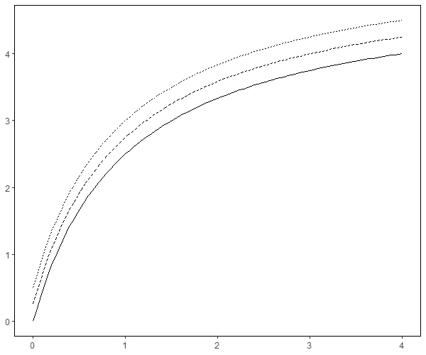
Some typical curves are displayed in Figure 1.

Refer to caption

Refer to caption

Figure 1: Typical E-max curves considered in the simulation study. Left panel: intersecting curves defined by (4.2) with γ=0\gamma=0 (solid), γ=2.7\gamma=2.7 (dashed) and γ=30\gamma=30 (dotted). Right panel: parallel curves defined by (4.3) with δ=0\delta=0 (solid), δ=1/4\delta=1/4 (dashed) and δ=1/2\delta=1/2 (dotted).

An equal number of observations is allocated to five equidistant dose levels x1,1=x2,1=0,x1,2=x2,2=1,…,x1,5=x2,5=4x_{1,1}=x_{2,1}=0,\thinspace x_{1,2}=x_{2,2}=1,\thinspace\ldots,\thinspace x_{1,5}=x_{2,5}=4, and the sample sizes for both groups are given by n1=n2=20,50,100n_{1}=n_{2}=20,50,100 and 200200. The errors in the regression models (2.1) are centered normal distributions with variances chosen as (σ12,σ22)=(0.25,0.25)(\sigma_{1}^{2},\sigma_{2}^{2})=(0.25,0.25) and (0.25,0.5)(0.25,0.5). All bootstrap results are obtained by B=300B=300 replications.

As estimators for the parameters in the regression models (2.1) we use least squares estimators, that is

βℓ^\displaystyle\hat{\beta_{\ell}} =\displaystyle= arg​minβℓ∈ℝpℓ​1nℓ​∑i=1kℓ∑j=1nℓ,i(Yℓ,i,j−mℓ​(xℓ,i,βℓ))2,\displaystyle{\rm arg}\min_{\beta_{\ell}\in\mathbb{R}^{p_{\ell}}}\dfrac{1}{n_{\ell}}\sum_{i=1}^{k_{\ell}}\sum_{j=1}^{n_{\ell,i}}(Y_{\ell,i,j}-m_{\ell}(x_{\ell,i},{\beta_{\ell}}))^{2}\penalty\ ,
σ^ℓ2\displaystyle\hat{\sigma}_{\ell}^{2} =\displaystyle= 1nℓ​∑i=1kℓ∑j=1nℓ,i(Yℓ,i,j−mℓ​(xℓ,i,βℓ^))2\displaystyle\dfrac{1}{n_{\ell}}\sum_{i=1}^{k_{\ell}}\sum_{j=1}^{n_{\ell,i}}(Y_{\ell,i,j}-m_{\ell}(x_{\ell,i},\hat{\beta_{\ell}}))^{2}\penalty\

(ℓ=1,2)(\ell=1,2). We start investigating the coverage probabilities of the asymptotic and bootstrap confidence intervals for the distance d1d_{1} defined in (2.10) and (3.2), respectively. For the asymptotic confidence interval we estimate the set 𝒩{\cal N} by (2.8) with c=1c=1. The parameters in the two E-max models (4.1) are defined by (4.2) and (4.3) such that d1=1d_{1}=1. The corresponding results are given in Table 1, where the upper part corresponds to the intersecting and the lower part to the parallel scenario. We observe that the coverage probabilities of the asymptotic confidence interval are too small, but they improve with increasing sample size. The results for the bootstrap confidence intervals are more satisfactory. For small sample sizes the bootstrap yields intervals with a too large coverage probability, but in general it provides an improvement.

(σ12,σ22)(\sigma_{1}^{2},\sigma_{2}^{2})
(n1,n2)(n_{1},n_{2}) (0.25, 0.25) (0.25, 0.5) (0.25, 0.25) (0.25, 0.5)
(20,20) 0.640 0.680 1.000 1.000
(50,50) 0.690 0.695 0.990 1.000
(100,100) 0.830 0.810 0.965 0.990
(200,200) 0.845 0.845 0.955 0.960
(20,20) 0.620 0.645 1.000 1.000
(50,50) 0.695 0.760 0.994 1.000
(100,100) 0.775 0.755 0.972 0.984
(200,200) 0.855 0.840 0.938 0.960
Table 1: Coverage probabilities of the asymptotic (left) and bootstrap 95%95\%-confidence interval (right). The regression functions are given by (4.1) such that d1=1d_{1}=1. Upper part: intersecting curves defined by (4.2). Lower part: parallel curves defined by (4.3).

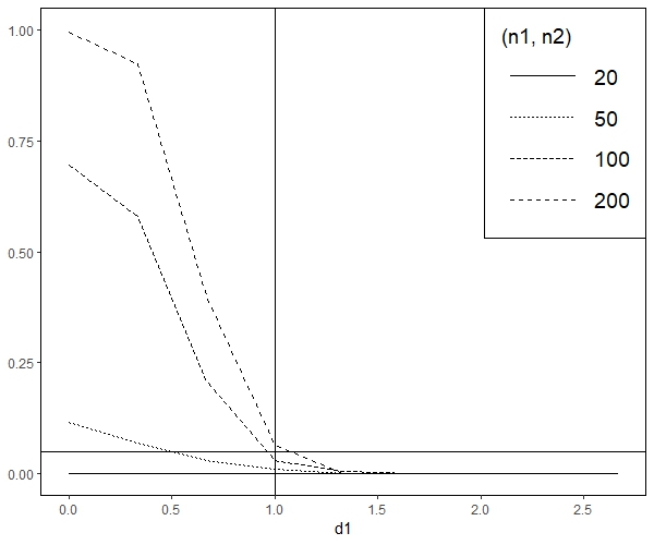
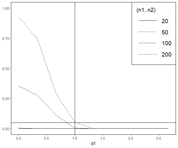
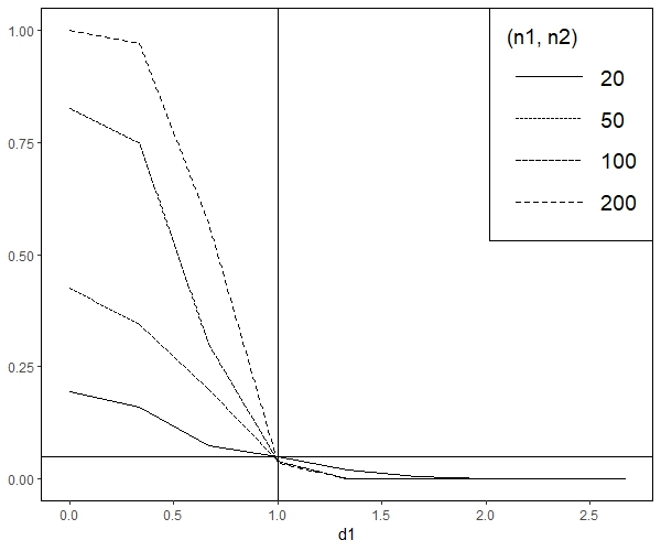
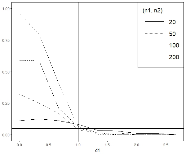
Next, we consider the problem of testing the hypotheses (2.3) with ϵ=1\epsilon=1. We begin with the two tests (2.11) and (3.3), which have been derived from the asymptotic and bootstrap confidence interval, respectively. The corresponding rejection probabilities are displayed in Figure 2 for the E-max models (4.1) with parameters (4.3) (parallel curves). Note that in this case d1=4​δd_{1}=4\delta and λ⁡(𝒩)=0\lambda(\mathcal{N})=0, whenever δ≠0\delta\not=0. Therefore, the cases δ≥0.25\delta\geq 0.25 and δ<0.25\delta<0.25 correspond to the null hypothesis and alternative in (2.3), respectively. The horizontal solid line marks the significance level α=0.05\alpha=0.05 and the vertical solid line corresponds to the boundary of the null hypothesis, that is d1=1d_{1}=1. The curves reflect the qualitative behaviour predicted by Theorem 2.2 and Theorem 3.1. Note that the power curves are decreasing in d1d_{1} as the null hypothesis is given by H0:d1≥1H_{0}:d_{1}\geq 1. We observe that the asymptotic test (2.11) does not keep its nominal level. In particular for small sample sizes the level is substantially exceeded. On the other hand, the bootstrap test (3.3) keeps the nominal level in all situations under consideration. The asymptotic test has more power, but this advantage comes at the cost of an unreliable approximation of the nominal level. Therefore, if one would have to choose from these tests, we would recommend to use the test based on the bootstrap confidence interval. Note that this test has not much power for the sample sizes n1=n2=20n_{1}=n_{2}=20 and 5050, but the constrained bootstrap test developed in Section 3 will yield a further improvement.

Refer to caption

Refer to caption Refer to caption Refer to caption

Figure 2: Rejection probabilities of the tests (2.11) (left) and (3.3) (right) for the hypotheses (2.3). First row: σ12=σ22=0.25\sigma_{1}^{2}=\sigma_{2}^{2}=0.25; Second row: σ12=0.25,\sigma_{1}^{2}=0.25, σ22=0.5\sigma_{2}^{2}=0.5. The nominal level is α=0.05\alpha=0.05 and parallel E-Max models defined by (4.3) are considered.
Refer to caption

Refer to caption Refer to caption Refer to caption

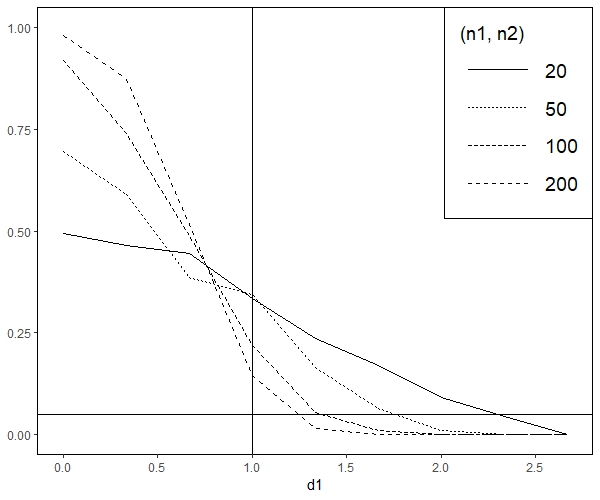
Figure 3: Rejection probabilities of the constrained bootstrap test (3.6) (Algorithm 2) for the hypotheses (2.3). Left panels: intersecting E-max models with parameters (4.2) Right panels: parallel E-max models with parameters (4.3). First row: σ12=σ22=0.25\sigma_{1}^{2}=\sigma_{2}^{2}=0.25; Second row: σ12=0.25,\sigma_{1}^{2}=0.25, σ22=0.5\sigma_{2}^{2}=0.5. The nominal level is α=0.05\alpha=0.05.

In Figure 3 we illustrate the performance of the test (3.6) (constrained bootstrap - see Algorithm 2) for testing the hypotheses (2.3) with ϵ=1\epsilon=1. The rejection probabilities for the situation investigated in Figure 2 (parallel E-Max models defined by (4.3)) are shown in the right part of the figure. These results are directly comparable with the right panels in Figure 2. We observe that the constrained bootstrap test (3.6) yields a substantial improvement in power compared to the test (3.3), which is based on the bootstrap confidence interval. For example, if d1=0d_{1}=0, n1=n2=50n_{1}=n_{2}=50, σ12=σ22=(0.25,0.25)\sigma_{1}^{2}=\sigma_{2}^{2}=(0.25,0.25), the test (3.3) has approximately power 0.1150.115, while the power of the constrained bootstrap test is 0.4550.455. The left part of the Figure 3 shows the results for intersecting E-Max models (defined by (4.2)). A comparison with the right part shows that the differences in power between the two cases (intersecting E-Max and shifted E-Max curves) are rather small.

5 Proofs

In this section we give proofs to all theoretical results in this work. For this purpose we require the following assumptions:

Assumption 1: The errors ηℓ,i,j\eta_{\ell,i,j} have finite variance σℓ2\sigma_{\ell}^{2} and mean 0.

Assumption 2: The covariate region 𝒳⊂ℝd\mathcal{X}\subset\mathbb{R}^{d} is compact and the number and location levels of kℓk_{\ell} does not depend on nℓn_{\ell} for ℓ=1,2\ell=1,2.

Assumption 3: All estimators of the parameters β1\beta_{1}, β2\beta_{2} are computed over compact sets B1⊂ℝp1B_{1}\subset\mathbb{R}^{p_{1}} and B2⊂ℝp2B_{2}\subset\mathbb{R}^{p_{2}}.

Assumption 4: The regression functions m1m_{1} and m2m_{2} are twice continuously differentiable with respect to the parameters for all b1,b2b_{1},b_{2} in the neighbourhoods of the true parameters β1,β2\beta_{1},\beta_{2} and all x∈𝒳x\in\mathcal{X}. The functions (x,bℓ)↣mℓ​(x,bℓ)(x,b_{\ell})\rightarrowtail m_{\ell}(x,b_{\ell}) and their first two derivatives are continuous on 𝒳×Bℓ\mathcal{X}\times B_{\ell} for ℓ=1,2\ell=1,2.

Assumption 5: Defining

ψa,ℓ(n)​(b)≔∑i=1kℓnℓ,inℓ​(mℓ​(xℓ,i,a)−mℓ​(xℓ,i,b))2,\psi^{(n)}_{a,\ell}(b)\coloneqq\sum_{i=1}^{k_{\ell}}\dfrac{n_{\ell,i}}{n_{\ell}}(m_{\ell}(x_{\ell,i},a)-m_{\ell}(x_{\ell,i},b))^{2},

we assume that for any u>0u>0 there exists a constant vu,ℓ>0v_{u,\ell}>0 such that

lim infn→∞infa∈Bℓinf|b−a|≥uψa,ℓ(n)(b)≥vu,ℓ,ℓ=1,2.\liminf_{n\to\infty}\inf_{a\in B_{\ell}}\inf_{\left\lvert b-a\right\rvert\geq u}\psi^{(n)}_{a,\ell}(b)\geq v_{u,\ell},\ \ \ell=1,2.

Assumption 6: The matrices Σℓ\Sigma_{\ell} are non-singular and the sample sizes n1,n2n_{1},n_{2} converge to infinity such that

limnℓ→∞nℓ,inℓ=ξℓ,i>0,i=1,…,kℓ,ℓ=1,2.\lim_{n_{\ell}\to\infty}\dfrac{n_{\ell,i}}{n_{\ell}}=\xi_{\ell,i}>0,\ \ i=1,\ldots,k_{\ell},\ \ell=1,2.

and

limn1,n2→∞nn1=κ∈(1,∞).\lim_{n_{1},n_{2}\to\infty}\dfrac{n}{n_{1}}=\kappa\in(1,\infty).

Assumption 7: We denote by β^1,β^2\hat{\beta}_{1},\hat{\beta}_{2} estimators of the parameters β1,β2\beta_{1},\beta_{2} and assume that they can be linearized, meaning the estimators fulfill the following condition:

nℓ(βℓ^−βℓ)=1nℓ∑i=1kℓ∑j=1nℓ,iϕℓ,i,j+oℙ(1) as nℓ→∞,ℓ=1,2\sqrt{n_{\ell}}(\hat{\beta_{\ell}}-\beta_{\ell})=\dfrac{1}{\sqrt{n_{\ell}}}\sum_{i=1}^{k_{\ell}}\sum_{j=1}^{n_{\ell,i}}\phi_{\ell,i,j}+o_{\mathbb{P}}(1)\ \text{ as }n_{\ell}\to\infty,\ \ell=1,2

with square integrable influence functions ϕ1,i,j\phi_{1,i,j} and ϕ2,i,j\phi_{2,i,j} satisfying

𝔼[ϕℓ,i,j]=0,j=1,…,nℓ,i,i=1,…,kℓ,ℓ=1,2.\mathbb{E}[\phi_{\ell,i,j}]=0,\ j=1,\ldots,n_{\ell,i},\ i=1,\ldots,k_{\ell},\ \ell=1,2.

This implies that the asymptotic distribution of β1^\hat{\beta_{1}} and β2^\hat{\beta_{2}} is given by

nℓ(βℓ^−βℓ)→𝑑𝒩(0,Σℓ−1),ℓ=1,2,\sqrt{n_{\ell}}(\hat{\beta_{\ell}}-\beta_{\ell})\xrightarrow{d}\mathcal{N}(0,\Sigma_{\ell}^{-1}),\ \ell=1,2,

where the asymptotic covariance matrix is given by

Σℓ−1=∑i=1kℓξℓ,i𝔼[ϕℓ,i,jϕℓ,i,j⊤],ℓ=1,2.\Sigma_{\ell}^{-1}=\sum_{i=1}^{k_{\ell}}\xi_{\ell,i}\mathbb{E}[\phi_{\ell,i,j}\phi_{\ell,i,j}^{\top}],\ \ell=1,2.

Moreover, the variance estimators σ^12\hat{\sigma}_{1}^{2} and σ^22\hat{\sigma}_{2}^{2} used in (2.7) are consistent.

5.1 Proof of Theorem 2.1

We will prove this result by an application of the (functional) delta method for directionally differentiable functionals as stated in Theorem 2.1 in Shapiro, 1991. We introduce the notations θ⁡(x)=m1​(x,β1)−m2​(x,β2)\theta(x)=m_{1}(x,\beta_{1})-m_{2}(x,\beta_{2}), θ^​(x)=m1​(x,β^1)−m2​(x,β^2),\hat{\theta}(x)=m_{1}(x,\hat{\beta}_{1})-m_{2}(x,\hat{\beta}_{2}), θ={θ⁡(x)}x∈𝒳\theta=\{\theta(x)\}_{x\in{\cal X}} and θ^={θ^​(x)}x∈𝒳\hat{\theta}=\{\hat{\theta}(x)\}_{x\in{\cal X}}, and will show below that the mapping

Φ:{ℓ∞​(𝒳)→ℝf→Φ⁡(f)=∫𝒳|f⁡(x)|​𝑑x\displaystyle\Phi:\begin{cases}&\ell^{\infty}(\mathcal{X})\to\mathbb{R}\\ &f\to\Phi(f)=\int_{\mathcal{X}}\left\lvert f(x)\right\rvert\thinspace dx\end{cases}

is directionally Hadamard differentiable with respect to the L1L^{1}-norm on ℓ∞​(𝒳)\ell^{\infty}(\mathcal{X}) and the absolute value norm on ℝ\mathbb{R}, where the derivative is given by

Φh′:{ℓ∞​(𝒳)→ℝf→Φh′(f)=∫{h≠0}sgn(h(x))f(x)dx+∫{h=0}|f(x)|dx\Phi_{h}^{{}^{\prime}}:\penalty\ \begin{cases}&\ell^{\infty}(\mathcal{X})\to\mathbb{R}\\ &f\to\Phi_{h}^{{}^{\prime}}(f)=\int_{\{h\neq 0\}}\operatorname{sgn}(h(x))f(x)\thinspace dx\ +\int_{\{h=0\}}\left\lvert f(x)\right\rvert\thinspace dx\end{cases}

at h∈ℓ∞​(𝒳)h\in\ell^{\infty}(\mathcal{X}). Note that (ℓ∞​(𝒳),‖⋅‖1)\left(\ell^{\infty}(\mathcal{X}),\left\lVert\cdot\right\rVert_{1}\right) is still separable and that its norm is weaker than the sup-norm.

Hence the convergence in distribution

n​{θ^​(x)−θ⁡(x)}x∈𝒳→𝑑{G⁡(x)}x∈𝒳\displaystyle\sqrt{n}\big\{\hat{\theta}(x)-\theta(x)\big\}_{x\in\mathcal{X}}\xrightarrow{d}\{G(x)\}_{x\in\mathcal{X}}

in (ℓ∞​(𝒳),‖⋅‖∞)\left(\ell^{\infty}(\mathcal{X}),\left\lVert\cdot\right\rVert_{\infty}\right) established in Dette et al., 2018 is also valid in this setting. In particular, applying the (directional) delta method (Theorem 2.1 in Shapiro, 1991) gives

n​(d^1−d1)\displaystyle\sqrt{n}(\hat{d}_{1}-d_{1}) OPEN=n​∫𝒳|θ^​(x)|−|θ⁡(x)|​𝑑x=n​(Φ⁡({θ^​(x)}x∈𝒳)−Φ⁡({θ⁡(x)}x∈𝒳)))\displaystyle=\sqrt{n}\int_{\mathcal{X}}\ |{\hat{\theta}(x)}|-\left\lvert\theta(x)\right\rvert\ dx=\sqrt{n}\left(\Phi(\{\hat{\theta}(x)\}_{x\in\mathcal{X}})-\Phi(\{\theta(x)\}_{x\in\mathcal{X}}))\right)
→𝑑Φθ′({G(x)}x∈𝒳)=∫𝒩csgn(θ(x))G(x)dx+∫𝒩|G(x)|dx,\displaystyle\xrightarrow{d}\Phi^{{}^{\prime}}_{\theta}(\{G(x)\}_{x\in\mathcal{X}})=\int_{{{\cal N}}^{c}}\operatorname{sgn}(\theta(x))\ G(x)\ dx+\int_{{{\cal N}}}\left\lvert G(x)\right\rvert\ dx,

where 𝒩{{\cal N}} is defined in (2.5). Therefore, we are left with showing the differentiability of the functional Φ\Phi. For this purpose we write Φ=Φ1∘Φ2,\Phi=\Phi_{1}\circ\Phi_{2}, where

Φ1:\displaystyle\Phi_{1}: {ℓ∞​(𝒳)→ℝf→Φ1​(f)=∫𝒳f⁡(x)​𝑑x,Φ2:{ℓ∞​(𝒳)→ł∞​(𝒳)Φ2​(f)=|f|\displaystyle\begin{cases}&\ell^{\infty}(\mathcal{X})\to\mathbb{R}\\ &f\to\Phi_{1}(f)=\int_{\mathcal{X}}f(x)dx\end{cases}\penalty\ ,\penalty\ \penalty\ \penalty\ \penalty\ \Phi_{2}:\begin{cases}&\ell^{\infty}(\mathcal{X})\to\l^{\infty}(\mathcal{X})\\ &\Phi_{2}(f)=\left\lvert f\right\rvert\end{cases}

As a linear mapping Φ1\Phi_{1} is obviously Hadamard differentiable with derivative (Φ1)h′=Φ1(\Phi_{1})_{h}^{{}^{\prime}}=\Phi_{1} at h∈ℓ∞​(𝒳)h\in\ell^{\infty}(\mathcal{X}), where the latter is equipped with the L1L_{1} norm. We prove below that Φ2\Phi_{2} is directionally Hadamard differentiable with respect to the L1L^{1}-norm on ℓ∞​(𝒳)\ell^{\infty}(\mathcal{X}) and derivative

(Φ2)h′:{ℓ∞​(𝒳)→ℓ∞​(𝒳)f→(Φ2)h′(f)=𝟙{h≠0}sgn(h)f+𝟙{h=0}|f|\displaystyle(\Phi_{2})_{h}^{{}^{\prime}}:\begin{cases}&\ell^{\infty}(\mathcal{X})\to\ell^{\infty}(\mathcal{X})\\ &f\to(\Phi_{2})_{h}^{{}^{\prime}}(f)=\mathbbm{1}_{\{h\neq 0\}}\operatorname{sgn}(h)f+\mathbbm{1}_{\{h=0\}}\left\lvert f\right\rvert\end{cases} (5.1)

at h∈ℓ∞​(𝒳)h\in\ell^{\infty}(\mathcal{X}). The assertion then follows by the chain rule given in Proposition 3.6 in Shapiro, 1990.

For a proof of (5.1) let (xn)(x_{n}) be a sequence in ł∞​(𝒳)\l^{\infty}(\mathcal{X}) converging to xx and (tn)(t_{n}) be a sequence of positive real numbers converging to zero. We show that

‖Φ2​(h+tn​xn)−Φ2​(h)tn−(Φ2)h′(x)‖1→n→∞0,\left\lVert\frac{\Phi_{2}(h+t_{n}x_{n})-\Phi_{2}(h)}{t_{n}}-(\Phi_{2})_{h}^{{}^{\prime}}(x)\right\rVert_{1}\xrightarrow{n\to\infty}0, (5.2)

where

Zn=Φ2​(h+tn​xn)−Φ2​(h)tn−(Φ2)h′(x).Z_{n}=\frac{\Phi_{2}(h+t_{n}x_{n})-\Phi_{2}(h)}{t_{n}}-(\Phi_{2})_{h}^{{}^{\prime}}(x)\penalty\ .

This proves the claim.

For a proof of (5.2) note that this statement is equivalent to

(A2.1) Zn→𝜆0,\displaystyle\penalty\ \penalty\ \penalty\ \penalty\ \penalty\ \penalty\ \ Z_{n}\xrightarrow{\lambda}0\penalty\ ,
(A2.2) (Zn)​ is uniformly integrable ,\displaystyle\penalty\ \penalty\ \penalty\ \penalty\ \penalty\ \penalty\ \ (Z_{n})\text{ is uniformly integrable },

where →𝜆\xrightarrow{\lambda} denotes λ\lambda-stochastic convergence (Bauer, 2011, see Theorem 21.4 and the preceding definitions in).

Proof (A2.1). To prove this statement, it suffices to show that every subsequence (Znk)(Z_{n_{k}}) of (Zn)(Z_{n}) has a further subsequence (Znkj)(Z_{n_{k_{j}}}) which converges to zero almost everywhere. So let (Znk)(Z_{n_{k}}) be a subsequence of (Zn)(Z_{n}). Since xn→‖⋅‖1xx_{n}\xrightarrow{\left\lVert\cdot\right\rVert_{1}}x by assumption, we know that xnk→‖⋅‖1xx_{n_{k}}\xrightarrow{\left\lVert\cdot\right\rVert_{1}}x. Theorem 15.7 in Bauer, 2011 then implies that there exists a subsequence (xnkj)(x_{n_{k_{j}}}) such that xnkj→a.exx_{n_{k_{j}}}\xrightarrow{a.e}x. We conclude that Znkj→a.e0Z_{n_{k_{j}}}\xrightarrow{a.e}0 by the following:

  • 1)

    On the set {t∈ℝ∣xnkj(t)→x(t),h(t)=0}\{t\in\mathbb{R}\mid x_{n_{k_{j}}}(t)\to x(t),\ h(t)=0\} we have

    Znkj​(t)=|xnkj​(t)|−|x⁡(t)|→j→∞0.Z_{n_{k_{j}}}(t)=\big|{x_{n_{k_{j}}}(t)}\big|-\left\lvert x(t)\right\rvert\xrightarrow{j\to\infty}0.
  • 2)

    On the set {t∈ℝ∣xnkj(t)→x(t),h(t)>0}\{t\in\mathbb{R}\mid x_{n_{k_{j}}}(t)\to x(t),\ h(t)>0\} we have for sufficiently large jj

    Znkj​(t)=xnkj​(t)−x⁡(t)→j→∞0.Z_{n_{k_{j}}}(t)=x_{n_{k_{j}}}(t)-x(t)\xrightarrow{j\to\infty}0.
  • 3)

    On the set {t∈ℝ∣xnkj(t)→x(t),h(t)<0}\{t\in\mathbb{R}\mid x_{n_{k_{j}}}(t)\to x(t),\ h(t)<0\} we have for sufficiently large jj

    Znkj​(t)=−xnkj​(t)+x⁡(t)→j→∞0.Z_{n_{k_{j}}}(t)=-x_{n_{k_{j}}}(t)+x(t)\xrightarrow{j\to\infty}0.

Proof (A2.2). We have that

|Zn|\displaystyle\left\lvert Z_{n}\right\rvert =||h+tn​xn|−|h|tn−(Φ2)h′(x)|≤||h+tn​xn|−|h|tn|+|(Φ2)h′(x)|\displaystyle=\left\lvert\frac{\left\lvert h+t_{n}x_{n}\right\rvert-\left\lvert h\right\rvert}{t_{n}}-(\Phi_{2})_{h}^{{}^{\prime}}(x)\right\rvert\leq\left\lvert\frac{\left\lvert h+t_{n}x_{n}\right\rvert-\left\lvert h\right\rvert}{t_{n}}\right\rvert+\left\lvert(\Phi_{2})_{h}^{{}^{\prime}}(x)\right\rvert
≤|h+tn​xn−h|tn+|x|=|xn|+|x|\displaystyle\leq\frac{\left\lvert h+t_{n}x_{n}-h\right\rvert}{t_{n}}+\left\lvert x\right\rvert=\left\lvert x_{n}\right\rvert+\left\lvert x\right\rvert

where we have used the definition of (Φ2)h′(\Phi_{2})_{h}^{{}^{\prime}} for the second inequality. Now |xn|\left\lvert x_{n}\right\rvert is uniformly integrable, since xn→‖⋅‖1xx_{n}\xrightarrow{\left\lVert\cdot\right\rVert_{1}}x and |x|\left\lvert x\right\rvert is uniformly integrable, since xx is bounded. Therefore |xn|+|x|\left\lvert x_{n}\right\rvert+\left\lvert x\right\rvert is uniformly integrable. Since |Zn|\left\lvert Z_{n}\right\rvert is dominated by |xn|+|x|\left\lvert x_{n}\right\rvert+\left\lvert x\right\rvert, the result follows.

5.2 Proof of Theorem 2.2

We first show that, unconditionally,

T^→ℙT.\displaystyle\hat{T}\xrightarrow{\mathbb{P}}T\penalty\ . (5.3)

For this purpose we note that it follows from Assumption 1-7 that

∥θ−θ^∥∞=Oℙ(n−1/2).\displaystyle\|{\theta-\hat{\theta}}\|_{\infty}=O_{\mathbbm{P}}(n^{-1/2}). (5.4)

Next we define

S:=∫𝒩csgn⁡θ⁡(x)​G^​(x)​𝑑x+∫𝒩|G^​(x)|​𝑑x\displaystyle S:=\int_{{\cal N}^{c}}\operatorname{sgn}\theta(x)\ \hat{G}(x)\ dx+\int_{{\cal N}}|\hat{G}(x)|\ dx

and let λ\lambda denote the Lebesgue measure on 𝒳\mathcal{X}. By the triangle inequality we have

|T−T^|≤|T−S|+|S−T^|.\displaystyle|{T-\hat{T}}|\leq\left\lvert T-S\right\rvert+|{S-\hat{T}}|.

Note that {G^​(x)−G​(x)}x∈𝒳\left\{\hat{G}(x)-G(x)\right\}_{x\in\mathcal{X}} tends to 0∈(ℓ∞​(𝒳),‖⋅‖∞)0\in(\ell_{\infty}(\mathcal{X}),\left\lVert\cdot\right\rVert_{\infty}) in probability by Slutsky’s Theorem, which implies

|S−T|≤‖G^−G‖1≤λ⁡(𝒳)​‖G^−G‖∞,|S-T|\leq\|{\hat{G}-G}\|_{1}\leq\lambda(\mathcal{X})\|{\hat{G}-G}\|_{\infty}\penalty\ ,

and as a consequence |T−S|→0\left\lvert T-S\right\rvert\to 0 in probability. We are hence left with showing that |S−T^|→0|{S-\hat{T}}|\to 0 in probability. To this end we observe

|S−T^|≤A+B\displaystyle|S-\hat{T}|\leq A+B

where

A\displaystyle A =|∫𝒩^csgn⁡(θ^​(x))​G^​(x)​𝑑x−∫𝒩csgn⁡(θ⁡(x))​G^​(x)​𝑑x|\displaystyle=\Big|\int_{\hat{\mathcal{N}}^{c}}\operatorname{sgn}(\hat{\theta}(x))\thinspace\hat{G}(x)\ dx\ -\int_{\mathcal{N}^{c}}\operatorname{sgn}(\theta(x))\thinspace\hat{G}(x)\ dx\Big|
B\displaystyle B =|∫𝒩^|G^​(x)​|𝑑x−∫𝒩|G^​(x)|​𝑑x|\displaystyle=\Big|\int_{\hat{\mathcal{N}}}|\hat{G}(x)|\ dx\ -\int_{\mathcal{N}}|\hat{G}(x)|\ dx\Big|

We will only show that A→0A\to 0 in probability, the corresponding result for BB follows by similar arguments. Note that

A\displaystyle A ≤|∫𝒩^c∩𝒩sgn⁡(θ^​(x))​G^​(x)​𝑑x−∫𝒩c∩𝒩^sgn⁡(θ⁡(x))​G^​(x)​𝑑x|\displaystyle\leq\Big|\int_{\hat{\mathcal{N}}^{c}\cap\mathcal{N}}\operatorname{sgn}(\hat{\theta}(x))\thinspace\hat{G}(x)\ dx-\int_{\mathcal{N}^{c}\cap\hat{\mathcal{N}}}\operatorname{sgn}(\theta(x))\thinspace\hat{G}(x)\ dx\Big|
+|∫𝒩c∩𝒩^c(sgn⁡(θ^​(x))−sgn⁡(θ⁡(x)))​G^​(x)​𝑑x|\displaystyle\quad\quad+\Big|\int_{\mathcal{N}^{c}\cap\hat{\mathcal{N}}^{c}}\big(\operatorname{sgn}(\hat{\theta}(x))-\operatorname{sgn}(\theta(x))\big)\hat{G}(x)dx\Big|
≤λ⁡(𝒩^c∩𝒩)​‖G^‖∞+λ⁡(𝒩c∩𝒩^)​‖G^‖∞+oℙ​(1),\displaystyle\leq\lambda(\hat{\mathcal{N}}^{c}\cap\mathcal{N})\|{\hat{G}}\|_{\infty}+\lambda(\mathcal{N}^{c}\cap\hat{\mathcal{N}})\|{\hat{G}}\|_{\infty}+o_{\mathbbm{P}}(1)\penalty\ ,

where the last inequality is true because with high probability the signs in the third integral cancel each other other out on 𝒩^c∩𝒩c\hat{\mathcal{N}}^{c}\cap\mathcal{N}^{c}. This can be seen by recalling the definition of the set 𝒩c\mathcal{N}^{c} and equation (5.4). The other two terms vanish due to G^​(x)\hat{G}(x) being bounded in probability by virtue of its tightness and because

λ⁡(𝒩^c∩𝒩)\displaystyle\lambda(\hat{\mathcal{N}}^{c}\cap\mathcal{N}) =λ({x|θ^(x)≥clog⁡(n)/n,θ(x)=0})\displaystyle=\lambda\big(\{x\penalty\ |\penalty\ \hat{\theta}(x)\geq c\sqrt{\log(n)/n},\theta(x)=0\}\big)
≤λ⁡({x|n​(θ^​(x)−θ⁡(x))≥c​log⁡(n)})=oℙ​(1)\displaystyle\leq\lambda\big(\{x\penalty\ |\penalty\ \sqrt{n}(\hat{\theta}(x)-\theta(x))\geq c\log(n)\}\big)=o_{\mathbbm{P}}(1)

due to (5.4). As a similar inequality holds true for the set 𝒩c∩𝒩^\mathcal{N}^{c}\cap\hat{\mathcal{N}}, this concludes the proof of (5.3).

Define 𝒴:={Yℓ,i,j:ℓ=1,2,i=1,…,kℓ,j=1,…,nℓ,i}\mathcal{Y}:=\{Y_{\ell,i,j}:\ell=1,2,\ i=1,...,k_{\ell},\ j=1,\ldots,n_{\ell,i}\}, consider the conditional distribution ℙT^|𝒴\mathbb{P}^{\hat{T}|\mathcal{Y}} and note that by the previous argument we have

ℙ⁡(T^−T∈𝒜)=∫ℙT^−T|𝒴​(𝒜)​𝑑ℙ→0\displaystyle\mathbb{P}(\hat{T}-T\in\mathcal{A})=\int\mathbb{P}^{\hat{T}-T|\mathcal{Y}}(\mathcal{A})d\mathbb{P}\rightarrow 0

which implies that T^−T|𝒴→0\hat{T}-T|\mathcal{Y}\rightarrow 0 in probability by a suitable choice of a countable family of 𝒜\mathcal{A} and a repeated subsequence argument. We hence obtain that q^0,α\hat{q}_{0,\alpha} converges to qαq_{\alpha} in probability. As all quantities of which we take limits in the following are real valued we may assume WLOG that it does so even almost surely.
Observe that

ℙ⁡(d1∈[0,d^1−q^0,αn])\displaystyle\mathbb{P}\Big(d_{1}\in[0,\hat{d}_{1}-\dfrac{\hat{q}_{0,\alpha}}{\sqrt{n}}]\Big) =1−ℙ⁡(n​(d^1−d1)≤q^0,α)\displaystyle=1-\mathbb{P}\Big(\sqrt{n}(\hat{d}_{1}-d_{1})\leq\hat{q}_{0,\alpha}\Big)
=1−ℙ⁡(n​(d^1−d1)≤qα+o⁡(1))\displaystyle=1-\mathbb{P}\Big(\sqrt{n}(\hat{d}_{1}-d_{1})\leq q_{\alpha}+o(1)\Big)

By Egorovs Theorem we may assume that the o(1) term vanishes uniformly on a set of measure δ\delta for any δ>0\delta>0, to be precise for n⁡(m)n(m) large enough we have o⁡(1)≤1/mo(1)\leq 1/m on a set 𝒜m\mathcal{A}_{m} that has measure at least 1−1/m1-1/m. Hence for n≥n⁡(m)n\geq n(m) we obtain

ℙ⁡(n​(d^1−d1)≤qα+o⁡(1))\displaystyle\mathbb{P}\Big(\sqrt{n}(\hat{d}_{1}-d_{1})\leq q_{\alpha}+o(1)\Big) ≤ℙ⁡(n​(d^1−d1)≤qα+1/m,𝒜m)+ℙ⁡(𝒜mc)\displaystyle\leq\mathbb{P}\Big(\sqrt{n}(\hat{d}_{1}-d_{1})\leq q_{\alpha}+1/m,\mathcal{A}_{m}\Big)+\mathbb{P}(\mathcal{A}_{m}^{c})
≤ℙ⁡(n​(d^1−d1)≤qα+1/m)+1/m\displaystyle\leq\mathbb{P}\Big(\sqrt{n}(\hat{d}_{1}-d_{1})\leq q_{\alpha}+1/m\Big)+1/m

A similar lower bound can be obtained by the same arguments. Letting nn go to infinity then establishes

ℙ⁡(d1∈[0,d^1−q^0,αn])=1−ℙ⁡(n​(d^1−d1)≤q^0,α)→1−α\displaystyle\mathbb{P}\Big(d_{1}\in[0,\hat{d}_{1}-\dfrac{\hat{q}_{0,\alpha}}{\sqrt{n}}]\Big)=1-\mathbb{P}\Big(\sqrt{n}(\hat{d}_{1}-d_{1})\leq\hat{q}_{0,\alpha}\Big)\rightarrow 1-\alpha

because the convergence of the distribution functions of n​(d^1−d1)\sqrt{n}(\hat{d}_{1}-d_{1}) is uniform for all continuity points of FTF_{T}.

This proves the first part of Theorem 2.2.

For the test in (2.11) we have under the null hypothesis H0:d1≥ϵH_{0}:d_{1}\geq\epsilon that ϵ−d1≤0\epsilon-d_{1}\leq 0, which implies for the probability of rejection

ℙ⁡(d^1<ϵ+q^0,αn)\displaystyle\mathbb{P}\Big(\hat{d}_{1}<\epsilon+\dfrac{\hat{q}_{0,\alpha}}{\sqrt{n}}\Big) =ℙ⁡(n​(d^1−d1)<n​(ϵ−d1)+q^0,α)\displaystyle=\mathbb{P}(\sqrt{n}(\hat{d}_{1}-d_{1})<\sqrt{n}(\epsilon-d_{1})+\hat{q}_{0,\alpha})
≤ℙ⁡(n​(d^1−d1)<q^0,α)\displaystyle\leq\mathbb{P}(\sqrt{n}(\hat{d}_{1}-d_{1})<\hat{q}_{0,\alpha})
=ℙ⁡(n​(d^1−d1)<qα−(qα−q^0,α))→n→∞α,\displaystyle=\mathbb{P}(\sqrt{n}(\hat{d}_{1}-d_{1})<q_{\alpha}-(q_{\alpha}-\hat{q}_{0,\alpha}))\xrightarrow{n\to\infty}\alpha,

where the convergence follows from similar arguments as for the first part of the theorem and Theorem 2.1. Consequently, the decision rule (2.11) defines an asymptotic level α\alpha-test. Similarly, under the alternative, we have ϵ−d1>0\epsilon-d_{1}>0, which yields consistency, that is

ℙ⁡(d^1<ϵ+q^0,αn)\displaystyle\mathbb{P}\Big(\hat{d}_{1}<\epsilon+\dfrac{\hat{q}_{0,\alpha}}{\sqrt{n}}\Big) =ℙ⁡(n​(d^1−d1)<n​(ϵ−d1)+q^0,α)→n→∞1,\displaystyle=\mathbb{P}(\sqrt{n}(\hat{d}_{1}-d_{1})<\sqrt{n}(\epsilon-d_{1})+\hat{q}_{0,\alpha})\xrightarrow{n\to\infty}1,

since q^0,α→ℙqα\hat{q}_{0,\alpha}\xrightarrow{\mathbb{P}}q_{\alpha} and n​(ϵ−d1)→n→∞∞\sqrt{n}(\epsilon-d_{1})\xrightarrow{n\to\infty}\infty imply n​(ϵ−d1)+q^0,α→n→∞∞\sqrt{n}(\epsilon-d_{1})+\hat{q}_{0,\alpha}\xrightarrow{n\to\infty}\infty and we know that n​(d^1−d1)\sqrt{n}(\hat{d}_{1}-d_{1}) converges in distribution by Theorem 2.1.

5.3 Proof of Theorem 3.1

We start with proving the properties of the test. We have

ℙ⁡(q^1−α,0∗<ϵ)\displaystyle\mathbb{P}\big(\hat{q}_{1-\alpha,0}^{*}<\epsilon\big) =ℙ⁡(n​(q^1−α,0∗−d^1)<n​(ϵ−d1)+n​(d1−d^1))\displaystyle=\mathbb{P}\big(\sqrt{n}(\hat{q}_{1-\alpha,0}^{*}-\hat{d}_{1})<\sqrt{n}(\epsilon-d_{1})+\sqrt{n}(d_{1}-\hat{d}_{1})\big)

Following the arguments in the proof of Theorem 2 of Dette et al., 2018 (where we use Theorem 23.9 from Van der Vaart, 2000 instead of an explicit first order expansion and the continuous mapping theorem) we obtain that

n​(q^1−α,0∗−d^1)→ℙq1−α\displaystyle\sqrt{n}(\hat{q}_{1-\alpha,0}^{*}-\hat{d}_{1})\xrightarrow{\mathbb{P}}q_{1-\alpha} (5.5)

where q1−αq_{1-\alpha} is the 1−α1-\alpha quantile of the Random Variable TT defined in (2.6). Since n​(d1−d^1)\sqrt{n}(d_{1}-\hat{d}_{1}) converges in distribution to TT by Theorem 2.1, TT is symmetric when λ⁡(𝒩)=0\lambda(\mathcal{N})=0, n​(ϵ−d1)\sqrt{n}(\epsilon-d_{1}) converges to zero if d1=ϵd_{1}=\epsilon and to ±∞\pm\infty in the alternative/remainder of the null hypothesis, we obtain the desired statement on the significance level and the consistency of the test.

For the confidence interval we observe that

ℙ⁡(d1∈I^n∗)\displaystyle\mathbb{P}\big(d_{1}\in\hat{I}_{n}^{*}\big) =ℙ⁡(d1<q^1−α,0∗)=ℙ⁡(n​(d1−d^1)<n​(q^1−α,0∗−d^1))\displaystyle=\mathbb{P}\big(d_{1}<\hat{q}_{1-\alpha,0}^{*}\big)=\mathbb{P}\big(\sqrt{n}(d_{1}-\hat{d}_{1})<\sqrt{n}(\hat{q}_{1-\alpha,0}^{*}-\hat{d}_{1})\big)

which yields the desired statement by (5.2).

5.4 Proof of Theorem 3.3

Proof of a). First, we determine the asymptotic distribution of the bootstrap test statistic d^1∗\hat{d}_{1}^{*}. Define θ^∗​(x)=m1​(x,β^1∗)−m2​(x,β^2∗)\hat{\theta}^{*}(x)=m_{1}(x,\hat{\beta}_{1}^{*})-m_{2}(x,\hat{\beta}_{2}^{*}) and θ^^​(x)=m1​(x,β^^1)−m2​(x,β^^2)\hat{\hat{\theta}}(x)=m_{1}(x,\hat{\hat{\beta}}_{1})-m_{2}(x,\hat{\hat{\beta}}_{2}). Following the proof of Theorem 1 in Dette et al., 2018 yields that conditionally on 𝒴\mathcal{Y} in probability

{n​(θ^∗​(x)−θ^^​(x))}x∈𝒳→𝑑{G⁡(x)}x∈𝒳.\displaystyle\big\{\sqrt{n}\big(\hat{\theta}^{*}(x)-\hat{\hat{\theta}}(x)\big)\big\}_{x\in\mathcal{X}}\xrightarrow{d}\{G(x)\}_{x\in\mathcal{X}}.

By assumption the directional hadamard derivative Φθ′\Phi^{\prime}_{\theta} is linear and thus a proper hadamard derivative which allows us to apply the delta method for the bootstrap as stated in Theorem 23.9 in Van der Vaart, 2000. Consequently we obtain

n​(d^1∗−d^^1)\displaystyle\sqrt{n}\big(\hat{d}_{1}^{*}-\hat{\hat{d}}_{1}\big) =n(Φ({θ^∗(x)}x∈𝒳)−Φ({θ^^(x)}x∈𝒳))→𝑑Φθ′({G(x)}x∈𝒳)\displaystyle=\sqrt{n}\big(\Phi(\{\hat{\theta}^{*}(x)\}_{x\in\mathcal{X}})-\Phi(\{\hat{\hat{\theta}}(x)\}_{x\in\mathcal{X}})\big)\xrightarrow{d}\Phi^{{}^{\prime}}_{\theta}(\{G(x)\}_{x\in\mathcal{X}})

conditionally on 𝒴\mathcal{Y} in probability.

Case 1: d1>ϵd_{1}>\epsilon. We observe that

ℙ⁡(d^1<q^α,1∗)\displaystyle\mathbb{P}(\hat{d}_{1}<\hat{q}_{\alpha,1}^{*}) =\displaystyle= ℙ⁡(d^1<q^α,1∗,d^1≥ϵ)+ℙ⁡(d^1<q^α,1∗,d^1<ϵ)\displaystyle\mathbb{P}(\hat{d}_{1}<\hat{q}_{\alpha,1}^{*}\ ,\hat{d}_{1}\geq\epsilon)+\mathbb{P}(\hat{d}_{1}<\hat{q}_{\alpha,1}^{*}\ ,\hat{d}_{1}<\epsilon)\ (5.6)
≤\displaystyle\leq ℙ⁡(d^1<q^α,1∗,d^^1=d^1)+ℙ⁡(d^1<ϵ)\displaystyle\mathbb{P}(\hat{d}_{1}<\hat{q}_{\alpha,1}^{*}\ ,\hat{\hat{d}}_{1}=\hat{d}_{1})+\mathbb{P}(\hat{d}_{1}<\epsilon)
≤\displaystyle\leq ℙ⁡(d^^1<q^α,1∗)+ℙ⁡(n​(d^1−d1)<n​(ϵ−d1)).\displaystyle\mathbb{P}(\hat{\hat{d}}_{1}<\hat{q}_{\alpha,1}^{*})+\mathbb{P}(\sqrt{n}(\hat{d}_{1}-d_{1})<\sqrt{n}(\epsilon-d_{1})).

We now show that the first sequence in the upper bound (5.6) converges to zero. To prove this, first note that for all α∈(0,1)\alpha\in(0,1)

n​(q^α,1∗−d^^1)→ℙqα,\displaystyle\sqrt{n}\ (\hat{q}_{\alpha,1}^{*}-\hat{\hat{d}}_{1})\xrightarrow{\mathbb{P}}q_{\alpha}, (5.7)

where qαq_{\alpha} denotes the α\alpha-quantile of the random variable TT defined in (2.6). To see this, observe that

α\displaystyle\alpha =\displaystyle= ℙ⁡(d^1∗<q^α,1∗∣𝒴)=ℙ⁡(n​(d^1∗−d^^1)<n​(q^α,1∗−d^^1)∣𝒴)​ a.s .\displaystyle\mathbb{P}(\hat{d}_{1}^{*}<\hat{q}_{\alpha,1}^{*}\mid\mathcal{Y})=\mathbb{P}(\sqrt{n}\thinspace(\hat{d}_{1}^{*}-\hat{\hat{d}}_{1})<\sqrt{n}(\hat{q}_{\alpha,1}^{*}-\hat{\hat{d}}_{1})\mid\mathcal{Y})\ \text{ a.s }.

Since n​(d^1∗−d^^1)\sqrt{n}(\hat{d}_{1}^{*}-\hat{\hat{d}}_{1}) converges in distribution to TT conditionally on 𝒴\mathcal{Y} in probability, Lemma 21.2 in Van der Vaart, 2000 yields the result (5.7). Using (5.7) and choosing α>0\alpha>0 small enough such that qα<0q_{\alpha}<0, we obtain

ℙ⁡(d^^1<q^α,1∗)\displaystyle\mathbb{P}(\hat{\hat{d}}_{1}<\hat{q}_{\alpha,1}^{*}) =\displaystyle= ℙ⁡(n​(q^α,1∗−d^^1)>0)≤ℙ⁡(|n​(q^α,1∗−d^^1)−qα|>−qα)→n→∞0.\displaystyle\mathbb{P}(\sqrt{n}(\hat{q}_{\alpha,1}^{*}-\hat{\hat{d}}_{1})>0)\leq\mathbb{P}\big(\big|{\sqrt{n}(\hat{q}_{\alpha,1}^{*}-\hat{\hat{d}}_{1})-q_{\alpha}}\big|>-q_{\alpha}\big)\xrightarrow{n\to\infty}0.

Finally, we show that the second sequence in the upper bound (5.6) converges to zero. Since d1>ϵd_{1}>\epsilon by assumption, we have that n​(ϵ−d1)→−∞\sqrt{n}(\epsilon-d_{1})\to-\infty and from Theorem 2.1 we know that n​(d^1−d1)\sqrt{n}(\hat{d}_{1}-d_{1}) converges in distribution. Therefore, the result follows. This concludes the proof of a) in the case d1>ϵd_{1}>\epsilon.

Case 2: d1=ϵd_{1}=\epsilon. We observe that

ℙ⁡(d^1<q^α,1∗)\displaystyle\mathbb{P}(\hat{d}_{1}<\hat{q}_{\alpha,1}^{*}) =\displaystyle= ℙ⁡(d^1<q^α,1∗,d^1≥ϵ)+ℙ⁡(d^1<q^α,1∗,d^1<ϵ)\displaystyle\mathbb{P}(\hat{d}_{1}<\hat{q}_{\alpha,1}^{*}\ ,\hat{d}_{1}\geq\epsilon)+\mathbb{P}(\hat{d}_{1}<\hat{q}_{\alpha,1}^{*}\ ,\hat{d}_{1}<\epsilon)
=\displaystyle= ℙ⁡(d^1<q^α,1∗,d^^1=d^1)+ℙ⁡(d^1<q^α,1∗,d^^1=ϵ)−ℙ⁡(d^1<q^α,1∗,d^1=ϵ)\displaystyle\mathbb{P}(\hat{d}_{1}<\hat{q}_{\alpha,1}^{*}\ ,\hat{\hat{d}}_{1}=\hat{d}_{1})+\mathbb{P}(\hat{d}_{1}<\hat{q}_{\alpha,1}^{*}\ ,\hat{\hat{d}}_{1}=\epsilon)-\mathbb{P}(\hat{d}_{1}<\hat{q}_{\alpha,1}^{*}\ ,\hat{d}_{1}=\epsilon)
=\displaystyle= ℙ(d^1<q^α,1∗,d^^1=d^1)+ℙ(d^1<q^α,1∗,d^^1=ϵ=d1)+o(1)\displaystyle\mathbb{P}(\hat{d}_{1}<\hat{q}_{\alpha,1}^{*}\ ,\hat{\hat{d}}_{1}=\hat{d}_{1})+\mathbb{P}(\hat{d}_{1}<\hat{q}_{\alpha,1}^{*}\ ,\hat{\hat{d}}_{1}=\epsilon=d_{1})+o(1)
=\displaystyle= ℙ⁡(n​(d^1−d1)<n​(q^α,1∗−d^^1),d^^1=ϵ)+o⁡(1)\displaystyle\mathbb{P}(\sqrt{n}(\hat{d}_{1}-d_{1})<\sqrt{n}(\hat{q}_{\alpha,1}^{*}-\hat{\hat{d}}_{1})\ ,\hat{\hat{d}}_{1}=\epsilon)+o(1)
=\displaystyle= ℙ⁡(n​(d^1−d1)<n​(q^α,1∗−d^^1))\displaystyle\mathbb{P}(\sqrt{n}(\hat{d}_{1}-d_{1})<\sqrt{n}(\hat{q}_{\alpha,1}^{*}-\hat{\hat{d}}_{1}))
−ℙ(d^1−d1<q^α,1∗−d^^1,d^^1>ϵ)+o(1).\displaystyle-\mathbb{P}(\hat{d}_{1}-d_{1}<\hat{q}_{\alpha,1}^{*}-\hat{\hat{d}}_{1}\ ,\hat{\hat{d}}_{1}>\epsilon)+o(1).

Because of (5.7) and Theorem 2.1, we have that

ℙ⁡(n​(d^1−d1)<n​(q^α,1∗−d^^1))→n→∞α.\displaystyle\mathbb{P}(\sqrt{n}(\hat{d}_{1}-d_{1})<\sqrt{n}(\hat{q}_{\alpha,1}^{*}-\hat{\hat{d}}_{1}))\xrightarrow{n\to\infty}\alpha.

Since d^^1>ϵ\hat{\hat{d}}_{1}>\epsilon implies d^1−d1>0\hat{d}_{1}-d_{1}>0 and (5.7) holds, we obtain

ℙ(d^1−d1<q^α,1∗−d^^1,d^^1>ϵ)≤ℙ(0<q^α,1∗−d^^1)→n→∞0,\displaystyle\mathbb{P}(\hat{d}_{1}-d_{1}<\hat{q}_{\alpha,1}^{*}-\hat{\hat{d}}_{1}\ ,\hat{\hat{d}}_{1}>\epsilon)\leq\mathbb{P}(0<\hat{q}_{\alpha,1}^{*}-\hat{\hat{d}}_{1})\xrightarrow{n\to\infty}0,

which completes the proof of a).

Proof of b). The result follows by the same arguments as given for the proof of the second statement of Theorem 2 in Dette et al., 2018. Only note that the map (b1,b2)↦d1​(b1,b2)(b_{1},b_{2})\mapsto d_{1}(b_{1},b_{2}) from B1×B2B_{1}\times B_{2} onto ℝ\mathbb{R} is uniformly continuous, since it is a continuous function on a compact set.

5.5 Proof of the statement in Remark 3.4(b)

Consider first the null hypothesis H0:d1≥ϵH_{0}:d_{1}\geq\epsilon. From Lemma 5.1 and Theorem 3.2 in Fang and Santos, 2019 we know that conditionally in probability

nΦ^′∗:=Φ^′({n(θ^∗−θ^)}x∈𝒳)→𝑑Φθ′({G(x)}x∈𝒳)=T.\displaystyle\sqrt{n}\thinspace\hat{\Phi}^{{}^{\prime}*}:=\hat{\Phi}^{{}^{\prime}}(\{\sqrt{n}(\hat{\theta}^{*}-\hat{\theta})\}_{x\in\mathcal{X}})\xrightarrow{d}\Phi^{{}^{\prime}}_{\theta}(\{G(x)\}_{x\in\mathcal{X}})=T.

Case 1: d1>ϵd_{1}>\epsilon. First note that for all α∈(0,1)\alpha\in(0,1) we have

n​q^α,1∗→ℙqα,\displaystyle\sqrt{n}\ \hat{q}_{\alpha,1}^{*}\xrightarrow{\mathbb{P}}q_{\alpha}, (5.8)

where qαq_{\alpha} denotes the α\alpha-quantile of TT and q^α,1∗\hat{q}_{\alpha,1}^{*} denotes the α\alpha-quantile of Φ^′∗\hat{\Phi}^{{}^{\prime}*}. To see this, observe that by definition of q^α,1∗\hat{q}_{\alpha,1}^{*} we have

α\displaystyle\alpha =\displaystyle= ℙ(Φ^′∗<q^α,1∗∣𝒴)=ℙ(nΦ^′∗<nq^α,1∗∣𝒴) a.s.\displaystyle\mathbb{P}(\hat{\Phi}^{{}^{\prime}*}<\hat{q}_{\alpha,1}^{*}\mid\mathcal{Y})=\mathbb{P}(\sqrt{n}\thinspace\hat{\Phi}^{{}^{\prime}*}<\sqrt{n}\thinspace\hat{q}_{\alpha,1}^{*}\mid\mathcal{Y})\ \text{ a.s. }

Since nΦ^′∗\sqrt{n}\thinspace\hat{\Phi}^{{}^{\prime}*} converges in distribution to TT conditionally on 𝒴\mathcal{Y} in probability, Lemma 21.2 in Van der Vaart, 2000 yields the result (5.8). Using (5.8) we then obtain that n​(q^α,1∗+ϵ−d1)→n→∞−∞\sqrt{n}(\hat{q}_{\alpha,1}^{*}+\epsilon-d_{1})\xrightarrow{n\to\infty}-\infty, since d1>ϵd_{1}>\epsilon. Combining this result with the fact that n​(d^1−d1)\sqrt{n}(\hat{d}_{1}-d_{1}) converges in distribution by Theorem 2.1, we can conclude that

ℙ⁡(d^1<q^α,1∗+ϵ)\displaystyle\mathbb{P}(\hat{d}_{1}<\hat{q}_{\alpha,1}^{*}+\epsilon) =ℙ⁡(n​(d^1−d1)<n​(q^α,1∗+ϵ−d1))→n→∞0.\displaystyle=\mathbb{P}(\sqrt{n}(\hat{d}_{1}-d_{1})<\sqrt{n}(\hat{q}_{\alpha,1}^{*}+\epsilon-d_{1}))\xrightarrow{n\to\infty}0.

Case 2: d1=ϵd_{1}=\epsilon. Since n​(d^1−d1)\sqrt{n}(\hat{d}_{1}-d_{1}) converges in distribution to TT and (5.8) holds, we deduce that

ℙ⁡(d^1<q^α,1∗+ϵ)\displaystyle\mathbb{P}(\hat{d}_{1}<\hat{q}_{\alpha,1}^{*}+\epsilon) =\displaystyle= ℙ⁡(n​(d^1−d1)<n​(q^α,1∗+ϵ−d1))\displaystyle\mathbb{P}(\sqrt{n}(\hat{d}_{1}-d_{1})<\sqrt{n}(\hat{q}_{\alpha,1}^{*}+\epsilon-d_{1}))
=\displaystyle= ℙ⁡(n​(d^1−d1)<n​q^α,1∗)→n→∞α.\displaystyle\mathbb{P}(\sqrt{n}(\hat{d}_{1}-d_{1})<\sqrt{n}\thinspace\hat{q}_{\alpha,1}^{*})\xrightarrow{n\to\infty}\alpha.

Next we consider the alternative H1:d1<ϵH_{1}:d_{1}<\epsilon. Using (5.8) and d1<ϵd_{1}<\epsilon, we deduce that n​(q^α,1∗+ϵ−d1)→n→∞∞\sqrt{n}(\hat{q}_{\alpha,1}^{*}+\epsilon-d_{1})\xrightarrow{n\to\infty}\infty. Since n​(d^1−d1)\sqrt{n}(\hat{d}_{1}-d_{1}) converges in distribution, this implies that

ℙ⁡(d^1<q^α,1∗+ϵ)\displaystyle\mathbb{P}(\hat{d}_{1}<\hat{q}_{\alpha,1}^{*}+\epsilon) =ℙ⁡(n​(d^1−d1)<n​(q^α,1∗+ϵ−d1))→n→∞1.\displaystyle=\mathbb{P}(\sqrt{n}(\hat{d}_{1}-d_{1})<\sqrt{n}(\hat{q}_{\alpha,1}^{*}+\epsilon-d_{1}))\xrightarrow{n\to\infty}1.
Lemma 5.1.

The sequence of functions

Φ^′(h)≔∫|θ^|≥1/snsgn(θ^(x))h(x)dx+∫|θ^|<1/sn|h(x)|dx\displaystyle\hat{\Phi}^{{}^{\prime}}(h)\coloneqq\int_{|{\hat{\theta}}|\geq{1}/s_{n}}\operatorname{sgn}(\hat{\theta}(x))\thinspace h(x)\ dx\ +\int_{|{\hat{\theta}}|<{1}/s_{n}}\left\lvert h(x)\right\rvert\ dx

with sn/n→0s_{n}/\sqrt{n}\to 0 satisfies Assumption 4 in Fang and Santos, 2019, meaning for h∈ł∞​(𝒳)h\in\l^{\infty}(\mathcal{X}) we have

|Φ^′(h)−Φθ′(h)|→ℙ0.\displaystyle\big|{\hat{\Phi}^{{}^{\prime}}(h)-\Phi_{\theta}^{{}^{\prime}}(h)}\big|\xrightarrow{\mathbb{P}}0.

(note that since Φ^′\hat{\Phi}^{{}^{\prime}} is Lipschitz continuous with respect to ‖⋅‖1\left\lVert\cdot\right\rVert_{1}, it suffices to prove this simpler condition; see Fang and Santos, 2019).

Proof.

Defining

A\displaystyle A ≔|∫|θ^|≥1/snsgn⁡(θ^​(x))​h​(x)​𝑑x−∫|θ|>0sgn⁡(θ⁡(x))​h​(x)​𝑑x|\displaystyle\coloneqq\Big|{\int_{|{\hat{\theta}}|\geq{1}/{s_{n}}}\operatorname{sgn}(\hat{\theta}(x))\thinspace h(x)\ dx\ -\int_{\left\lvert\theta\right\rvert>0}\operatorname{sgn}(\theta(x))\thinspace h(x)\ dx}\Big|
B\displaystyle B ≔|∫|θ^|<1/sn|h⁡(x)|​𝑑x−∫|θ|=0|h⁡(x)|​𝑑x|\displaystyle\coloneqq\Big|{\int_{|{\hat{\theta}}|<{1}/{s_{n}}}\left\lvert h(x)\right\rvert\ dx-\int_{\left\lvert\theta\right\rvert=0}\left\lvert h(x)\right\rvert\ dx\ }\Big|

we note that |Φ^′(h)−Φθ′(h)|≤A+B\big|{\hat{\Phi}^{{}^{\prime}}(h)-\Phi_{\theta}^{{}^{\prime}}(h)}\big|\leq A+B by the triangle inequality. Therefore, it suffices to show that A→ℙ0A\xrightarrow{\mathbb{P}}0 and B→ℙ0B\xrightarrow{\mathbb{P}}0. In order to show the former (the latter can be proven by similar arguments), we define the sets

M1≔{|θ^|>1sn},M2≔{|θ|>0}M_{1}\coloneqq\Big\{|\hat{\theta}|>\dfrac{1}{s_{n}}\Big\},\quad M_{2}\coloneqq\Big\{\left\lvert\theta\right\rvert>0\Big\}

and note that

A≤\displaystyle A\leq |∫M1∩M2csgn⁡(θ^​(x))​h​(x)​𝑑x−∫M2∩M1csgn⁡(θ⁡(x))​h​(x)​𝑑x|\displaystyle\thinspace\thinspace\Big|{\int_{M_{1}\cap M_{2}^{c}}\operatorname{sgn}(\hat{\theta}(x))\thinspace h(x)\ dx\ -\int_{M_{2}\cap M_{1}^{c}}\operatorname{sgn}(\theta(x))\thinspace h(x)\ dx}\Big|
+|∫M1∩M2(sgn⁡(θ^​(x))−sgn⁡(θ⁡(x)))​h​(x)​𝑑x|\displaystyle\quad+\Big|{\int_{M_{1}\cap M_{2}}\Big(\operatorname{sgn}(\hat{\theta}(x))-\operatorname{sgn}(\theta(x))\Big)\thinspace h(x)\ dx}\Big|
≤\displaystyle\leq λ⁡(M1∩M2c)​‖h‖∞+λ⁡(M2∩M1c)​‖h‖∞+oℙ​(1).\displaystyle\thinspace\thinspace\lambda(M_{1}\cap M_{2}^{c})\left\lVert h\right\rVert_{\infty}+\lambda(M_{2}\cap M_{1}^{c})\thinspace\left\lVert h\right\rVert_{\infty}+o_{\mathbb{P}}(1). (5.9)

due to θ^→ℙθ\hat{\theta}\xrightarrow{\mathbb{P}}\theta and where λ\lambda denotes the Lebesgue measure. Therefore, it suffices to show that the first two summands in (5.9) converge to zero in probability. Regarding the first term, we have that

λ⁡(M1∩M2c)\displaystyle\lambda\Big(M_{1}\cap M_{2}^{c}\Big)\thinspace =λ⁡(|θ^|>1sn,θ=0)=λ⁡(sn​|θ^−θ|>1,θ=0)\displaystyle=\lambda\Big(|{\hat{\theta}}|>\frac{1}{s_{n}},\thinspace\theta=0\Big)=\lambda\Big(s_{n}|{\hat{\theta}-\theta}|>1,\thinspace\theta=0\Big)
≤λ⁡(sn​|θ^−θ|>1)=λ⁡(snn​n​|θ^−θ|>1),\displaystyle\leq\lambda\Big(s_{n}|{\hat{\theta}-\theta}|>1\Big)=\lambda\Big(\frac{s_{n}}{\sqrt{n}}\sqrt{n}|{\hat{\theta}-\theta}|>1\Big),

where the last term converges to zero, since sn/n→0s_{n}/\sqrt{n}\to 0 by assumption and since the sequence n​|θ^−θ|\sqrt{n}|{\hat{\theta}-\theta}| is tight. The second summand can be handled similarly.

∎

Acknowledgements: This research is supported by the European Union through the European Joint Programme on Rare Diseases under the European Union’s Horizon 2020 Research and Innovation Programme Grant Agreement Number 825575.

References

  • Aitchison, (1964) Aitchison, J. (1964). Confidence-region tests. Journal of the Royal Statistical Society, Series B, 26:462–476.
  • Bauer, (2011) Bauer, H. (2011). Measure and Integration Theory. de Gruyter.
  • Berger, (1982) Berger, R. L. (1982). Multiparameter hypothesis testing and acceptance sampling. Technometrics, 24:295–300.
  • Bradley, (1997) Bradley, A. P. (1997). The use of the area under the roc curve in the evaluation of machine learning algorithms. Pattern recognition, 30(7):1145–1159.
  • Chow and Liu, (1992) Chow, S.-C. and Liu, P.-J. (1992). Design and Analysis of Bioavailability and Bioequivalence Studies. Marcel Dekker, New York.
  • Cox and Czanner, (2016) Cox, T. and Czanner, G. (2016). A practical divergence measure for survival distributions that can be estimated from kaplan-meier curves. Statistics in Medicine, 35.
  • Dette et al., (2018) Dette, H., Möllenhoff, K., Volgushev, S., and Bretz, F. (2018). Equivalence of regression curves. Journal of the American Statistical Association, 113(522):711–729.
  • EMA, (2014) EMA (2014). Guideline on the investigation of bioequivalence. available at http://www.ema.europa.eu/docs/en_GB/document_library/Scientific_guideline/2010/01/WC500070039.pdf.
  • Fang and Santos, (2019) Fang, Z. and Santos, A. (2019). Inference on directionally differentiable functions. The Review of Economic Studies, 86(1):377–412.
  • Gsteiger et al., (2011) Gsteiger, S., Bretz, F., and Liu, W. (2011). Simultaneous confidence bands for nonlinear regression models with application to population pharmacokinetic analyses. Journal of Biopharmaceutical Statistics, 21(4):708–725.
  • Hauschke et al., (2007) Hauschke, D., Steinijans, V., and Pigeot, I. (2007). Bioequivalence Studies in Drug Development Methods and Applications. Statistics in Practice. John Wiley & Sons, New York.
  • Heller et al., (2016) Heller, G., Seshan, V. E., Moskowitz, C. S., and Gönen, M. (2016). Inference for the difference in the area under the ROC curve derived from nested binary regression models. Biostatistics, 18(2):260–274.
  • Jachno et al., (2019) Jachno, K., Heritier, S., and Wolfe, R. (2019). Are non-constant rates and non-proportional treatment effects accounted for in the design and analysis of randomised controlled trials? a review of current practice. BMC medical research methodology, 19(1):1–9.
  • Liu et al., (2009) Liu, W., Bretz, F., Hayter, A. J., and Wynn, H. P. (2009). Assessing non-superiority, non-inferiority of equivalence when comparing two regression models over a restricted covariate region. Biometrics, 65(4):1279–1287.
  • Liu et al., (2007) Liu, W., Hayter, A. J., and Wynn, H. P. (2007). Operability region equivalence: simultaneous confidence bands for the equivalence of two regression models over restricted regions. Biometrical Journal, 49(1):144–150.
  • McCaw et al., (2019) McCaw, Z. R., Yin, G., and Wei, L.-J. (2019). Using the restricted mean survival time difference as an alternative to the hazard ratio for analyzing clinical cardiovascular studies. Circulation, 140(17):1366–1368.
  • Möllenhoff et al., (2022) Möllenhoff, K., Dette, H., and Bretz, F. (2022). Testing for similarity of binary efficacy–toxicity responses. Biostatistics, 23(3):949–966.
  • Ostrovski, (2017) Ostrovski, V. (2017). Testing equivalence of multinomial distributions. Statistics & Probability Letters, 124:77–82.
  • Pepe et al., (2013) Pepe, M. S., Kerr, K. F., Longton, G., and Wang, Z. (2013). Testing for improvement in prediction model performance. Statistics in Medicine, 32(9):1467–1482.
  • Royston and Parmar, (2013) Royston, P. and Parmar, M. K. (2013). Restricted mean survival time: an alternative to the hazard ratio for the design and analysis of randomized trials with a time-to-event outcome. BMC Medical Research Methodology, 13(1):152.
  • Shapiro, (1990) Shapiro, A. (1990). On concepts of directional differentiability. Journal of optimization theory and applications, 66(3):477–487.
  • Shapiro, (1991) Shapiro, A. (1991). Asymptotic analysis of stochastic programs. Annals of Operations Research, 30(1):169–186.
  • U.S. Food and Drug Administration, (2003) U.S. Food and Drug Administration (2003). Guidance for industry: bioavailability and bioequivalence studies for orally administered drug products-general considerations. Food and Drug Administration, Washington, DC. available at http://www.fda.gov/downloads/Drugs/GuidanceComplianceRegulatoryInformation/Guidances/ucm070124.pdf.
  • Van der Vaart, (2000) Van der Vaart, A. W. (2000). Asymptotic Statistics. Cambridge University Press.