Long-term gravitational wave asteroseismology of supernova:
from core collapse to 20 seconds postbouncePreprint: APS/123-QED
Abstract
We use an asteroseismology method to calculate the frequencies of gravitational waves (GWs) in a long-term core-collapse supernova simulation, with a mass of 9.6 solar mass. The simulation, which includes neutrino radiation transport in general relativity is performed from core-collapse, bounce, explosion and cooling of protoneutron stars (PNSs) up to 20 s after the bounce self-consistently. Based on the hydrodynamics background, we calculate eigenmodes of the PNS oscillation through a perturbation analysis on fluid and metric. We classify the modes by the number of nodes and find that there are several eigenmodes. In the early phase before 1 s, there are a low-frequency -mode around 0.5 kHz, a mid-frequency -modes around 1 kHz, and high-frequency -modes above them. Beyond 1 second, the -modes drop too low in frequency and the -modes become too high to be detected by ground-based interferometers. However, the -mode persists at 1 kHz. We present a novel fitting formula for the ramp-up mode, comprising a mixture of -mode and -mode, using postbounce time as a fitting parameter. Our approach yields improved results for the long-term simulation compared to prior quadratic formulas. We also fit frequencies using combinations of gravitational mass, , and radius, , of the PNS. We test three types of fitting variables: compactness , surface gravity , and average density . We present results of the time evolution of each mode and the fitting for three different ranges, from 0.2 s to 1 s, 4 s, and 20 s for each formula. We then compare the deviation of the formulas from the eigenmodes to determine which fitting formula is the best. In conclusion, any combination of and fits the eigenmodes well to a similar degree. Comparing 3 variables in detail, the fitting with compactness is slightly the best among them. We also find that the fitting using less than 1 s of simulation data cannot be extrapolated to the long-term frequency prediction.
I Introduction
The gravitational wave (GW) is one of the most important prediction of general relativity, which was directly confirmed by the observation of the binary black hole merger, GW150914 Abbott et al. 2016. After the memorial event, increasing number of GW events have been observed from binary star systems including merger of two neutron stars and black hole-neutron star systems Abbott et al. 2021.
The next most promising targets for observation of GWs are supernova explosions, the origin of neutron stars and black holes. Supernovae (SNe) emit electromagnetic waves, neutrinos, and GWs, and the multimessenger observations can provide deep insight into the supernova interior (see Refs. Mezzacappa 2005; Janka 2012; Kotake et al. 2012; Burrows 2013; Foglizzo et al. 2015; Müller 2020; Smartt 2015; Maeda 2022 for reviews). Indeed, the first detection of neutrinos from SN 1987A Hirata et al. 1987; Bionta et al. 1987; Alexeyev et al. 1988 allowed us to estimate the total energy emitted by neutrinos being erg Sato and Suzuki 1987; Burrows 1988; Lattimer and Yahil 1989 and led to the conclusion that a neutron star (NS) formed inside supernova explosion and the released gravitational energy drives the explosion. When the next galactic supernova happens, GWs would also be detected Abdikamalov et al. 2021. Combining these independent pieces of information will lead to a breakthrough in the study of supernova explosions.
The GW asteroseismology, which is counterpart of regular light-based asteroseismology but with GW, has a potential to provide NS parameters Andersson and Kokkotas 1998; Sotani and Takiwaki 2016; Sotani et al. 2017; Sotani et al. 2019; Sotani 2020; Sotani and Takiwaki 2020a; Sotani and Takiwaki 2020b; Sotani and Takiwaki 2020c; Sotani et al. 2021; Torres-Forné et al. 2018; Torres-Forné et al. 2019a; Torres-Forné et al. 2019b; Torres-Forné et al. 2021; Bizouard et al. 2021; Westernacher-Schneider et al. 2019. NSs are expected to produce strong GWs from their typical oscillation modes, which is so-called eigenmodes. If these oscillation modes are observed in GWs, we will be able to extract the combination of the mass and radius of the NS. There are three different variations of fitting formulas for evolution of oscillation frequencies; the compactness , the surface gravity , and the average density . For instance, Sotani et al. (2021) Sotani et al. 2021 proposed a universal relation for models employing different nuclear equations of state based on the average density, while Torres-Forné et al. (2019) Torres-Forné et al. 2019b; Torres-Forné et al. 2021 proposed a comparable formula but using the average density for - and -modes and the surface gravity for -modes. There are also studies where postbounce time is used as a fitting variable. Morozova et al. (2018) Morozova et al. 2018 used fitting with postbounce time and reported that differences between equation of states showed up. Warren et al. (2020) Warren et al. 2020 investigated a correlation between an estimate of GW frequencies and neutrino emission.
| Authors | Year | Gravity | Fitting variables | Simulation time (s) | References |
|---|---|---|---|---|---|
| Sotani and Takiwaki | 2016 | Newtonian | No fitting | 1.0 | Sotani and Takiwaki 2016 |
| Sotani, Kuroda, Takiwaki and Kotake | 2017 | GR | 0.3 | Sotani et al. 2017 | |
| Morozova et al. | 2018 | Approx GR | Postbounce time | 1.5 | Morozova et al. 2018 |
| Torres-Forné et al. | 2019 | Approx GR/ GR | 1.2 | Torres-Forné et al. 2019b; Torres-Forné et al. 2021 | |
| Warren et al. | 2020 | Approx GR | Postbounce time | 4.0 | Warren et al. 2020 |
| Sotani, Takiwaki and Togashi | 2021 | Approx GR | 0.8 | Sotani et al. 2021 | |
| Sotani and Sumiyoshi | 2021 | GR | 1.4 | Sotani and Sumiyoshi 2021 | |
| Mori, Suwa and Takiwaki | 202e | GR | , Postbounce time | 20 | This work |
Table 1 summarizes previous studies. The number of the models in the general relativistic framework is limited and no simulations were performed beyond 10 s except this work. We have not known how long the fitting formulas are applicable. The motivation of this study is to discover long-term behavior of frequencies and find a fitting formula for long-term emission. Another importance of long-term simulation is related to the multimessenger astronomy. If galactic supernovae happen, neutrino events are observable for more than 20 s Suwa et al. 2019; Mori et al. 2020 so we need the same time prediction of GWs to check the correlation.
Our goal of this work is to discover the behavior of NS eigenmode frequencies and the connection of their properties. To accomplish this goal, this paper employs the long-term simulation of a supernova explosion and NS formation. We will utilize data from Ref. Mori et al. 2020, especially long-term (20 s) self-consistent simulations from the collapse of the iron core to the supernova explosion and the protoneutron star (PNS) cooling phase. The late period has the great advantage of allowing more precise modeling than the early period ( s), as the complex physical processes settle down. Recently, Refs. Suwa et al. 2019; Suwa et al. 2021; Nakazato et al. 2022; Suwa et al. 2022 have developed a method to extract the mass and radius of the NS based on theoretical estimates of neutrino emission in the late phase. Theoretical predictions of GW, on the other hand, have been focused on the early phase, since long-term multi-dimensional numerical simulation are needed to predict the GW.
In this paper, we will show long-term evolution of PNS eigenmodes, which are a source of GW emission, investigate which combination of mass and radius can fit - and - modes the most for a long time and discuss the possibility whether we can estimate late-time frequencies from early time fitting. Our PNS simulation considers the full general relativistic gravity and neutrino transport, and our mode analysis employs metric perturbations. These make our estimation quantitatively precise. Section II explains the neutrino-radiation hydrodynamics simulation and the method to estimate eigenmodes of GWs based on the simulation. Section III describes the results of the eigenmode analysis and fitting. We use three parameters (compactness, surface gravity, and average density) to fit eigenmodes. We also propose new fitting formula with respect to time after bounce and provide a discussion on which fitting formula is the best. Finally, we summarize our conclusion in Section IV. Note that we employ the signature as the Minkowski metric and adopt units of .
II Methods
This section describes how to estimate the frequency of eigenmodes from our supernova model. We first conduct core-collapse supernova (CCSN) simulation by solving the neutrino-radiation hydrodynamics equations and then calculate eigenmodes of the PNS based on the simulation results. The calculation of the eigenmodes allows us to compute leading order contribution to GW signals.
II.1 Neutrino-radiation hydrodynamics simulation
Our CCSN model is based on the model in Ref. Mori et al. 2020. The progenitor is 9.6 and zero-initial metallicity (A. Heger, private communication, 2016), which has been reported to explode not only in multidimensional simulations but also in spherical symmetric simulations Melson et al. 2015; Radice et al. 2017; Mori et al. 2020; Nakazato et al. 2021.
As Ref. Mori et al. 2020, we employ a public code, GR1D O’Connor and Ott 2010; O’Connor 2015 for our hydrodynamics simulation. The primitive variables in GR1D are density , specific internal energy , velocity and electron fraction . The metric used in GR1D is
| (1) |
where and are radius and time. and are a lapse and a shift function, which are written with functions of the potential and enclosed gravitational mass ,
| (2) | ||||
| (3) |
Those are given as
| (4) | ||||
| (5) | ||||
where is enthalpy with being pressure, is Lorentz factor with being the product of three-velocity and and is the stress-energy tensor component of neutrinos. Here, is determined by the matching condition. The metric must be connected to the Schwarztshild metric at the star’s surface, which leads to
| (6) |
where is the star’s radius.
In GR1D, the hydrodynamics equations are described as below,
| (7) |
where is a set of conserved values, is a set of flow values, is a set of source terms, and . To be specific, conserved values are given as
| (8) |
where
| (9) | ||||
| (10) | ||||
| (11) | ||||
| (12) |
The flux vector is
| (13) |
and the source and sink terms are
| (14) | |||
where , , , and are the contributions of neutrinos and are calculated through the neutrino transport.
GR1D is implemented with the M1 scheme Shibata et al. 2011 with multi-energy groups for neutrino-radiation transport. It solves the Boltzmann equation up to the first two moments and use an analytic closure for closing moment equations. The energy groups are logarithmically divided into 18 energies. The center value of the lowest energy group is 2 MeV and that of the highest energy group is 280 MeV. In this simulation, neutrino transport is calculated out to 600 km and neutrino information is read out at 500 km considering effects of the gravity.
Interactions between neutrinos and matter are calculated in advance as an opacity table with Nulib. 11 1 https://github.com/evanoconnor/NuLib Table 2 summarizes interactions used in the simulation. In the original opacity table, the bremsstrahlung is taken into account only for heavy-lepton neutrinos. That is, the interaction of is only included. Since we found that this approximation leads to unphysically high average energy of and at the late phase Mori et al. 2020, we reproduce the numerical table taking into account the reaction, .
II.2 Asteroseismology
In order to calculate eigenmodes of oscillations in PNSs, we employ the asteroseismology method. GREAT Torres-Forné et al. 2018; Torres-Forné et al. 2019a is open source software for GW asteroseismology in general relativity Torres-Forné et al. 2018. That is, the perturbations in the linear analysis both of fluid and metric are considered. The oscillation follows the next equations:
| (15) | ||||
| (16) | ||||
where and are longitudinal and transverse coefficients of eigenmodes respectively, is the frequency, is the sound speed, is the conformal factor, and are the adiabatic index. and are the relativistic Lamb frequency and relativistic Brunt- frequency and their definitions are
| (17) | ||||
| (18) |
where is the gravity defined as
| (19) |
and is the relativistic version of the Schwarzschild discriminant defined as
| (20) |
Finally, about the metric perturbations, and , they read
| (21) | ||||
| (22) |
In order to find frequencies, , these Eqs. (II.2), (II.2), (21) and (22) are integrated from the center of the star to the PNS surface (). The inner boundary condition is , and the outer boundary condition is as same as Eq. (7) in Ref. Sotani and Takiwaki 2020b. See also Eqs. (4)–(6) of Ref. Sotani and Takiwaki 2020b to convert the spherical polar coordinate of Eq. (1) into the isotropic coordinate used in GREAT Marek et al. 2006.
III Results
III.1 PNS properties
Before going to the argument of the GW signal, we briefly give the time evolution of PNS gravitational mass and radius, which are shown in Figure 1. We define the surface of the PNS at the radius where the density is . The blue and red lines with the right and the left axis show the radius and gravitational mass of the PNS, respectively.
The PNS radius (blue line) is larger than 100 km at the bounce and then rapidly shrinks to 13 km. The baryonic mass of PNS converges to 1.36 soon after the onset of the explosion. In such a light progenitor, the mass accretion rate is small and PNS mass is converged in the early phase. Although the baryonic mass is constant, the gravitational mass (red line) decreases due to the neutrino emission up to 1.26 at 20 s after the bounce. Those evolutions are consistent with other studies. For instance, our baryonic mass 1.36 is consistent with previous studies that used the same progenitor model Müller et al. 2013; Wanajo et al. 2018; Radice et al. 2017. Our gravitational mass at the last moment of the simulation, 1.26 is also consistent with an approximate estimate given in Ref. Radice et al. 2017.


III.2 Gravitational wave modes
Using the model introduced in Section II.1 and the method described in Section II.2, we calculate the oscillation modes of the entire PNS. In the following, we classify the modes into -modes, -mode and -modes. The modes are characterized by the number of nodes. If there is no node, we call it -mode and otherwise it is - or -modes. The physical difference between -modes and -modes is restoring force. The -modes are invoked by pressure and the -modes are driven by buoyancy. The frequency of the -mode is higher as the number of nodes increases. On the other hand, that of the -mode is inversely lower as the number of nodes increases. While this simple classification is also used in Refs. Sotani and Takiwaki 2016; Sotani et al. 2017; Morozova et al. 2018; Torres-Forné et al. 2018; Sotani 2020; Sotani et al. 2021; Sotani and Takiwaki 2020b, Refs. Torres-Forné et al. 2019a; Torres-Forné et al. 2019b employ different classification criteria, but this difference affects only the names of the modes and does not change the following discussion.
Roughly speaking, the -mode propagates near the surface of the star and the -mode propagates near the center of the star. Figure 2 shows transverse coefficients of the -mode (blue) and -mode (red) as functions of radius at 1 s after the bounce, wherein the indexes of the subscript are the number of nodes. The coefficients are normalized for their maximum values to be unity. There is a node at 15 km and a peak at 7 km in the -mode. In the -mode, there is no node except at the center and the of the -mode increases with the radius. There is a node at 14 km in the -mode and are two nodes at 11 km and 19 km. Both of the -modes also increases with the radius.
Following the simple mode identification, we show the time evolution of eigenmodes of GWs in Figure 3, which are calculated from time snapshots of our supernova simulation. We show them from 0.1 s after the bounce in this figure because matter motion around the bounce is dynamical and clearly deviated from the eigenmodes. There are the -mode (red), -mode (blue) and -modes (green) in Figure 3, where is the natural number and indicates the number of nodes.
The -mode has the lowest frequencies, the -mode is in the middle frequency range, and the -modes are the highest. The -mode frequencies gradually increase, reach the peak around 0.7 kHz at 0.55 s, slowly decrease and eventually pass through 0.5 kHz at 2 s. Such evolution is also seen in the previous studies, e.g., see Fig. 5 of Ref. Morozova et al. 2018 and Fig. 3 of Ref. Sotani et al. 2021. The frequencies of -modes increase and even the lowest -mode exceeds 3 kHz at 2 s. Higher -modes increase faster.
The frequencies of the -mode increase from 0.6 kHz to 0.9 kHz for the first 0.15 s, keep the value up to 0.5 s and then slowly increase again to 1.6 kHz at 20 s. There are avoided crossings between the lowest -mode and -mode around 0.2 s and between the -mode and the -mode around 0.5 s Morozova et al. 2018; Sotani and Takiwaki 2020c. Note that the term of “avoided crossing” means that the frequencies of two eigenmodes approach each other but they do not cross. In the following section, we focus on the -mode before the avoided crossing and the -mode after the avoided crossing.

III.3 Fitting
In this section, we propose new fitting formulas for the eigenmode frequencies that is based on the long-term general relativistic simulation (see Figure 3). We provide one fitting formula in terms of postbounce time and three types of fitting methods with respect to the mass and the radius of the PNS: , and , which mean compactness, surface gravity and average density, respectively. See Table 1 for the difference from the previous formulas.
We select so-called ramp-up mode that has avoided crossing Morozova et al. 2018; Sotani and Takiwaki 2020c, i.e., that is -mode before 0.76 s and the -mode after 0.76 s in our classification (see Figure 3). In the multi-dimensional simulation, this mode most clearly and ubiquitously appears, e.g., Refs. Murphy et al. 2009; Müller et al. 2013. In the most of previous studies, fitting of this mode is provided (see Table 1).
First, we use postbounce time as a fitting variable. Morozova et al. Morozova et al. 2018 employed quadratic functions to fit eigenmode frequencies with postbounce time. However, the quadratic function can fit curves but cannot fit constant values. Thus, we also propose a new fitting formula with respect to postbounce time. The function writes:
| (23) |
where is postbounce time measured in s and , , and are fitting parameters. This function is proportional to when is close to 0 and becomes constant when is large enough. The parameters determined in this study are shown in Table 3. We also fit with quadratic function for comparison with Morozova et al. (2018) Morozova et al. 2018 and our fitting parameters for the quadratic function are summarized in Table 4.
| Fitting range (s) | ||||
|---|---|---|---|---|
| 0.2-1 | ||||
| 0.2-4 | ||||
| 0.2-20 |
| Fitting range (s) | |||
|---|---|---|---|
| 0.2-1 | |||
| 0.2-4 | |||
| 0.2-20 |
 |
| Fitting range (s) | |||||
|---|---|---|---|---|---|
| 0.2-1 | |||||
| 0.2-4 | |||||
| 0.2-20 | |||||
Figure 4 shows the fitting results of Eqs. (23) (orange) and comparisons to quadratic equations (gray). We employ data after 0.2 s in postbounce time because there are no clear eigenmodes due to turbulence around the bounce before this time. Three panels represent the different fitting ranges of 0.2–1 (bottom), 0.2–4 (middle), and 0.2–20 s (top). In the bottom panel, the function fits the - and -modes well and the result of the quadratic equatiaon overlaps from 0.2 to 1.0 s. After 1 s, which is the extrapolated region, predicts the higher frequencies. The value is higher by 0.1 kHz at 10 s and by 0.15 kHz at 20 s. The extrapolation of the quadratic equation does not match the simulation and deviates after 1 s. As we mentioned above, the quadratic formula is suitable to fit curves but not appropriate for asymptotically constant lines. The middle panel shows the result of the fitting range spanning from 0.2 to 4 s. The matches the simulation overall but predicts a slightly smaller value in the extrapolated region. The difference is 0.02 kHz at 20 s. The quadratic function has behavior similar to that in the bottom panel. That is, the function matches before 4 s but falls down after 4 s. The way to fall down is slower than that of the fitting from 0.2 to 1 s. Finally, the top panel shows the result of the fitting range from 0.2 to 20 s. The perfectly matches the simulation and the quadratic function does not match the -mode and has a similar shape after 1 s.
Next, we fit the eigenmodes with three formulas whose variables are , and , which mean compactness, surface gravity and average density, respectively. The expression of fitting function is the same as Sotani et al. (2021) Sotani and Sumiyoshi 2021, i.e.,
| (24) |
where , , and are fitting parameters and the variable takes , or .
The three variables, , and behave in the same way. Figure 6 shows time evolution of the variables. In the early time, slopes are steep and gradually become flat in the late time. In the early time, the slope of is the steepest, that of is next and that of is the most modest. The normalization is determined with the value at 20 s.

We fit of Eq. (24) over the different three time ranges: 0.2–1 s, 0.2–2 s and 0.2–20 s in postbounce time as well. The fitting results are shown in Figure 5 and Table 5. Figure 5 shows the fitting lines in the fitting ranges as solid lines and their extrapolations as dashed lines. In the case of the fitting range from 0.2 to 1 s, which is shown in the bottom panel, all the three functions with fitting with , and are similar and they predict lower frequencies in late time. During the fitting range, they match the simulation well. However, in the extrapolated region, they gradually become lower. The behavior is the same for all the fitting variables. The rate of deviation of is the fastest, followed by and finally is the slowest.
In the case of the fitting range from 0.2 to 4 s, which is shown in the middle panel. The fitting results of all the variables almost entirely overlap. In the fitting region, they perfectly match the simulation. In the extrapolated region, the fitting functions predict a little smaller values. At 20 s, the value of the fitting functions is 1.5 kHz and smaller by 0.09 kHz than that of the simulation. At last, in the case of fitting from 0.2 to 20 s, that is, the case that we fit from beginning to end, the all functions reproduce the simulation result well.
III.4 Comparison with previous studies
Figure 7 compares our fitting formulas with previous studies of Refs. Sotani and Sumiyoshi 2021; Torres-Forné et al. 2019b. The horizontal axes are in the top panel and in the bottom panel. There are three solid lines of different fitting ranges in each panel. In the top panel, all of the fitting formulas are similar to each other below 1 kHz. Eq. (5) of Sotani et al. (2021) Sotani and Sumiyoshi 2021(gray dashed) leads to slightly higher frequencies overall. The fitting formula of Torres-Forné et al. (2019) Torres-Forné et al. 2019b; Torres-Forné et al. 2021 overlaps our long-term fitting results.
In the bottom panel, Eq. (3) of Sotani et al. (2021) Sotani and Sumiyoshi 2021 (gray dashed) also has higher frequencies than ours. Note that the simulation conditions of our work and previous studies are different, e.g., the progenitor model, treatment of gravity, and equation of state. It is not so strange that the fitting formulas are different as well. For example, Ref. Bizouard et al. 2021 estimates the error bar of the frequency as Hz using 18 different models (see their Figure 1).


III.5 Discussion on which fitting is the best
According to Figures 4 and 5, the functions in the fitting ranges can reproduce the simulation regardless of variables (except ) and the extrapolation becomes better as the fitting range becomes longer. This subsection provides a discussion on the fitting results. We here ensure which variable is suitable in detail and how long fitting range is needed.
We define the dimensionless deviation of fitting below:
| (25) |
where is postbounce time, is the simulation time, which is 20 s now, is the starting time of the integral, which is 0.2 s, shows eigenmode frequencies as a function of time and means fitting functions, . The fitting range is from 0.2 s to in postbounce time. The smaller value means that the fitting is more accurate.
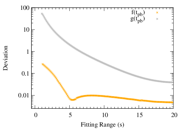
Figure 8 shows the deviations for functions of each variable from 1 s to 20 s in . The time bin is 0.005 s. The top panel compares Eq. (23) and the quadratic function. As discussed in the previous section, the quadratic function is not suitable for the long term fitting. Even if the fitting range is short (4 s), shows smaller deviation, which is 10%. The deviation of is about 0.25 at 1.5 s and gradually decreases to 0.008 at 20 s. can be used for the rough estimate for the whole evolution of the GW. The deviation using has a local minimum at 5 s. The fitting slowly converges after 7 s. A longer fitting range is necessary to obtain the precise estimate ( 1%). Note that, the fitting of depends on the initial guess. Before 6 s, we set as the initial guess and after 6 s. On the other hand, the deviation of the quadratic function is much larger. It has 60 at 1 s and decreases to 0.04 at 20 s, which corresponds to the deviation of at about 3 s.
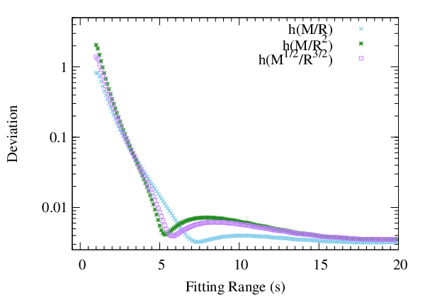
The bottom panel shows a comparison of fitting functions of Eq. (24) where the fitting parameters are , or . To keep the deviation below percent level, we need simulation for 4 s at least. All curves behave in a similar way regardless of fitting variables. The deviations monotonically decrease until 5 s ( 9 s for ) and keep below 0.01 after 5 s. Among the variables using and , the best fit would be . The deviation of fitting with has a maximum of 0.8 at 1 s, then decreases, has a local minimum of 0.003, raises twice, and finally converges to 0.003. The deviation of is the largest from 4 s to 6 s but the deviation is the smallest after 6 s. The deviations of fitting with and behave similarly. That of starts at 2 and has a dip of 0.004 around 5 s. Then, it has a peak of 0.007 at 7 s and converges to 0.004 again. Similarly, in the case of , the deviation is the biggest value of 1.5 at 1 s, has a dip of 0.0035 at 5 s, has a peak of 0.006 at 7 s and converges to 0.0035 at last.
IV Summary
In this paper, we calculated the frequencies of the eigenmodes of the PNS oscillation based on the long-term SN simulation and provided several fitting methods for the GW asteroseismology. The supernova model was simulated with GR1D, which solved the general relativistic neutrino radiation hydrodynamics equations. For the estimate of the frequencies of eigenmodes, we employed GREAT that calculates eigenmodes of PNS oscillations. The calculation continues up to 20 s, which is the longest compared with recent studies. we fitted the eigenmodes, which are the -mode before the avoided crossing and the -mode after it, with functions considering several types of fitting parameters.
We proposed the new fitting formula using the postbounce time, Eq. (23), and prove that it works better than the simple quadratic function. The quadratic function is suitable for fitting an increasing curve, and it falls short in accurately depicting an asymptotically constant one.
We also derived fitting equations using , , and as the previous studies Sotani et al. 2017; Torres-Forné et al. 2019b; Torres-Forné et al. 2021; Sotani et al. 2021; Sotani and Sumiyoshi 2021. These formulas effectively fit the eigenmodes, however, using leads to a slightly better long-term fit compared to the other two variables. Nevertheless, the difference is small, not making it a matter of choice between the variables. We also found that the fitting using less than 1 s of simulation data cannot be extrapolated to the long-term frequency prediction.
In order to give the quantitative behavior of the GW emission, we need to conduct multi-dimensional simulations Yokozawa et al. 2015; Kuroda et al. 2017; Andresen et al. 2017; O’Connor and Couch 2018; Radice et al. 2019; Mezzacappa et al. 2020; Nakamura et al. 2022; Andersen et al. 2021; Bugli et al. 2022; Bruel et al. 2023. The multi-dimensional simulation costs too many computational resources. However, Figure 8 indicates that simulations up to 5 s are enough for giving reliable GW predictions.
For future observations, our goal is to estimate properties of the supernova through the GWs. For this, we have to know inverse functions of eigenmode and of Eq. (24). Especially, in the late time, the turbulence of fluid subsides. If we use the late-time information, we can estimate the mass and the radius of the neutron star. In future work, we will prepare a lot of systematic simulations in order to make a template of eigenmodes and make extrapolations of radii and masses of neutron stars. The long-term template of eingenmodes and fluid properties allow us to quickly extract information on supernova interior. Moreover, in the case of a galactic supernova, we can also observe supernova neutrinos, which allow us to do multi-messenger astronomy. From a point of view of multi-messenger astronomy, it is worth estimating properties of SN and PNS independently with different messengers such as GWs and neutrinos. Indeed, there is a method to estimate PNS masses and radii from supernova neutrinos Suwa et al. 2022; Nagakura and Vartanyan 2022; Nakazato and Suzuki 2020. By combining neutrinos and GWs, we can check the consistency and give more reliable estimates than independent analysis. Since our supernova simulation includes the neutrino radiation transport, the combined analysis is possible, which will be reported in the future.
Acknowledgement
This work is supported by JSPS KAKENHI (JP18H01212, JP20H00174, JP20H01904, JP21H01088, JP22H01223) and Grant-in-Aid for Scientific Research on Innovative Areas (JP18H05437, JP20H04747, JP22H04571) from the Ministry of Education, Culture, Sports, Science and Technology (MEXT), Japan. This work was supported by computer clusters in Center for Computational Astrophysics. This research was also supported by MEXT as ‘Program for Promoting researches on the Supercomputer Fugaku’ (towards a unified view of the universe: from large-scale structures to planets, JPMXP1020200109) and JICFuS.
References
- Abbott et al. (2016) B. P. Abbott et al. (LIGO Scientific Collaboration and Virgo Collaboration), Observation of Gravitational Waves from a Binary Black Hole Merger, Phys. Rev. Lett. 116, 061102 (2016), arXiv:1602.03837 [gr-qc] .
- Abbott et al. (2021) B. P. Abbott et al. (The LIGO Scientific Collaboration and the Virgo Collaboration and the KAGRA Collaboration), GWTC-3: Compact Binary Coalescences Observed by LIGO and Virgo During the Second Part of the Third Observing Run, arXiv e-prints , arXiv:2111.03606 (2021), arXiv:2111.03606 [gr-qc] .
- Mezzacappa (2005) A. Mezzacappa, ASCERTAINING THE CORE COLLAPSE SUPERNOVA MECHANISM: The State of the Art and the Road Ahead, Annual Review of Nuclear and Particle Science 55, 467 (2005).
- Janka (2012) H.-T. Janka, Explosion Mechanisms of Core-Collapse Supernovae, Annual Review of Nuclear and Particle Science 62, 407 (2012), arXiv:1206.2503 [astro-ph.SR] .
- Kotake et al. (2012) K. Kotake, T. Takiwaki, Y. Suwa, W. Iwakami Nakano, S. Kawagoe, Y. Masada, and S.-i. Fujimoto, Multimessengers from Core-Collapse Supernovae: Multidimensionality as a Key to Bridge Theory and Observation, Advances in Astronomy 2012, 428757 (2012), arXiv:1204.2330 [astro-ph.HE] .
- Burrows (2013) A. Burrows, Colloquium: Perspectives on core-collapse supernova theory, Reviews of Modern Physics 85, 245 (2013), arXiv:1210.4921 [astro-ph.SR] .
- Foglizzo et al. (2015) T. Foglizzo, R. Kazeroni, J. Guilet, F. Masset, M. González, B. K. Krueger, J. Novak, M. Oertel, J. Margueron, J. Faure, N. Martin, P. Blottiau, B. Peres, and G. Durand, The Explosion Mechanism of Core-Collapse Supernovae: Progress in Supernova Theory and Experiments, PASA 32, e009 (2015), arXiv:1501.01334 [astro-ph.HE] .
- Müller (2020) B. Müller, Hydrodynamics of core-collapse supernovae and their progenitors, arXiv e-prints , arXiv:2006.05083 (2020), arXiv:2006.05083 [astro-ph.SR] .
- Smartt (2015) S. J. Smartt, Observational Constraints on the Progenitors of Core-Collapse Supernovae: The Case for Missing High-Mass Stars, PASA 32, e016 (2015), arXiv:1504.02635 [astro-ph.SR] .
- Maeda (2022) K. Maeda, Stellar evolution, SN explosion, and nucleosynthesis, arXiv e-prints , arXiv:2210.00326 (2022), arXiv:2210.00326 [astro-ph.HE] .
- Hirata et al. (1987) K. Hirata et al. (Kamiokande-II), Observation of a Neutrino Burst from the Supernova SN 1987a, Phys. Rev. Lett. 58, 1490 (1987).
- Bionta et al. (1987) R. Bionta et al., Observation of a Neutrino Burst in Coincidence with Supernova SN 1987a in the Large Magellanic Cloud, Phys. Rev. Lett. 58, 1494 (1987).
- Alexeyev et al. (1988) E. N. Alexeyev, L. N. Alexeyeva, I. V. Krivosheina, and V. I. Volchenko, Detection of the neutrino signal from SN 1987A in the LMC using the INR Baksan underground scintillation telescope, Physics Letters B 205, 209 (1988).
- Sato and Suzuki (1987) K. Sato and H. Suzuki, Total energy of the neutrino burst from the supernova 1987A and the mass of the neutron star just born, Physics Letters B 196, 267 (1987).
- Burrows (1988) A. Burrows, Supernova neutrinos, Astrophys. J. 334, 891 (1988).
- Lattimer and Yahil (1989) J. M. Lattimer and A. Yahil, Analysis of the Neutrino Events from Supernova 1987A, The Astrophysical Journal 340, 426 (1989).
- Abdikamalov et al. (2021) E. Abdikamalov, G. Pagliaroli, and D. Radice, Gravitational waves from core-collapse supernovae, in Handbook of Gravitational Wave Astronomy (Springer Singapore, 2021) pp. 1–37.
- Andersson and Kokkotas (1998) N. Andersson and K. D. Kokkotas, Towards gravitational wave asteroseismology, MNRAS 299, 1059 (1998), arXiv:gr-qc/9711088 [gr-qc] .
- Sotani and Takiwaki (2016) H. Sotani and T. Takiwaki, Gravitational wave asteroseismology with protoneutron stars, Phys. Rev. D 94, 044043 (2016), arXiv:1608.01048 [astro-ph.HE] .
- Sotani et al. (2017) H. Sotani, T. Kuroda, T. Takiwaki, and K. Kotake, Probing mass-radius relation of protoneutron stars from gravitational-wave asteroseismology, Phys. Rev. D 96, 063005 (2017), arXiv:1708.03738 [astro-ph.HE] .
- Sotani et al. (2019) H. Sotani, T. Kuroda, T. Takiwaki, and K. Kotake, Dependence of the outer boundary condition on protoneutron star asteroseismology with gravitational-wave signatures, Phys. Rev. D 99, 123024 (2019), arXiv:1906.04354 [astro-ph.HE] .
- Sotani (2020) H. Sotani, Gravitational wave asteroseismology for low-mass neutron stars, Phys. Rev. D 102, 063023 (2020), arXiv:2008.09839 [astro-ph.HE] .
- Sotani and Takiwaki (2020a) H. Sotani and T. Takiwaki, Dimension dependence of numerical simulations on gravitational waves from protoneutron stars, Phys. Rev. D 102, 023028 (2020a), arXiv:2004.09871 [astro-ph.HE] .
- Sotani and Takiwaki (2020b) H. Sotani and T. Takiwaki, Accuracy of the relativistic Cowling approximation in protoneutron star asteroseismology, Phys. Rev. D 102, 063025 (2020b), arXiv:2009.05206 [astro-ph.HE] .
- Sotani and Takiwaki (2020c) H. Sotani and T. Takiwaki, Avoided crossing in gravitational wave spectra from protoneutron star, MNRAS 498, 3503 (2020c), arXiv:2008.00419 [astro-ph.HE] .
- Sotani et al. (2021) H. Sotani, T. Takiwaki, and H. Togashi, Universal relation for supernova gravitational waves, Phys. Rev. D 104, 123009 (2021), arXiv:2110.03131 [astro-ph.HE] .
- Torres-Forné et al. (2018) A. Torres-Forné, P. Cerdá-Durán, A. Passamonti, and J. A. Font, Towards asteroseismology of core-collapse supernovae with gravitational-wave observations - I. Cowling approximation, MNRAS 474, 5272 (2018), arXiv:1708.01920 [astro-ph.SR] .
- Torres-Forné et al. (2019a) A. Torres-Forné, P. Cerdá-Durán, A. Passamonti, M. Obergaulinger, and J. A. Font, Towards asteroseismology of core-collapse supernovae with gravitational wave observations - II. Inclusion of space-time perturbations, MNRAS 482, 3967 (2019a), arXiv:1806.11366 [astro-ph.HE] .
- Torres-Forné et al. (2019b) A. Torres-Forné, P. Cerdá-Durán, M. Obergaulinger, B. Müller, and J. A. Font, Universal Relations for Gravitational-Wave Asteroseismology of Protoneutron Stars, Phys. Rev. Lett. 123, 051102 (2019b), arXiv:1902.10048 [gr-qc] .
- Torres-Forné et al. (2021) A. Torres-Forné, P. Cerdá-Durán, M. Obergaulinger, B. Müller, and J. A. Font, Erratum: Universal Relations for Gravitational-Wave Asteroseismology of Protoneutron Stars [Phys. Rev. Lett. 123, 051102 (2019)], Phys. Rev. Lett. 127, 239901 (2021).
- Bizouard et al. (2021) M.-A. Bizouard, P. Maturana-Russel, A. Torres-Forné, M. Obergaulinger, P. Cerdá-Durán, N. Christensen, J. A. Font, and R. Meyer, Inference of protoneutron star properties from gravitational-wave data in core-collapse supernovae, Phys. Rev. D 103, 063006 (2021), arXiv:2012.00846 [gr-qc] .
- Westernacher-Schneider et al. (2019) J. R. Westernacher-Schneider, E. O’Connor, E. O’Sullivan, I. Tamborra, M.-R. Wu, S. M. Couch, and F. Malmenbeck, Multimessenger asteroseismology of core-collapse supernovae, Phys. Rev. D 100, 123009 (2019), arXiv:1907.01138 [astro-ph.HE] .
- Morozova et al. (2018) V. Morozova, D. Radice, A. Burrows, and D. Vartanyan, The gravitational wave signal from core-collapse supernovae, Astrophys. J. 861, 10 (2018), arXiv:1801.01914 [astro-ph.HE] .
- Warren et al. (2020) M. L. Warren, S. M. Couch, E. P. O’Connor, and V. Morozova, Constraining Properties of the Next Nearby Core-collapse Supernova with Multimessenger Signals, Astrophys. J. 898, 139 (2020), arXiv:1912.03328 [astro-ph.HE] .
- Sotani and Sumiyoshi (2021) H. Sotani and K. Sumiyoshi, Stability of the protoneutron stars towards black hole formation, Mon. Not. Roy. Astron. Soc. 507, 2766 (2021), arXiv:2108.02484 [astro-ph.HE] .
- Suwa et al. (2019) Y. Suwa, K. Sumiyoshi, K. Nakazato, Y. Takahira, Y. Koshio, M. Mori, and R. A. Wendell, Observing Supernova Neutrino Light Curves with Super-Kamiokande: Expected Event Number over 10 s, ApJ 881, 139 (2019), arXiv:1904.09996 [astro-ph.HE] .
- Mori et al. (2020) M. Mori, Y. Suwa, K. Nakazato, K. Sumiyoshi, M. Harada, A. Harada, Y. Koshio, and R. A. Wendell, Developing an end-to-end simulation framework of supernova neutrino detection, Progress of Theoretical and Experimental Physics 2021, 10.1093/ptep/ptaa185 (2020).
- Suwa et al. (2021) Y. Suwa, A. Harada, K. Nakazato, and K. Sumiyoshi, Analytic solutions for neutrino-light curves of core-collapse supernovae, Progress of Theoretical and Experimental Physics 2021, 013E01 (2021), arXiv:2008.07070 [astro-ph.HE] .
- Nakazato et al. (2022) K. Nakazato, F. Nakanishi, M. Harada, Y. Koshio, Y. Suwa, K. Sumiyoshi, A. Harada, M. Mori, and R. A. Wendell, Observing Supernova Neutrino Light Curves with Super-Kamiokande. II. Impact of the Nuclear Equation of State, ApJ 925, 98 (2022), arXiv:2108.03009 [astro-ph.HE] .
- Suwa et al. (2022) Y. Suwa, A. Harada, M. Harada, Y. Koshio, M. Mori, F. Nakanishi, K. Nakazato, K. Sumiyoshi, and R. A. Wendell, Observing Supernova Neutrino Light Curves with Super-Kamiokande. III. Extraction of Mass and Radius of Neutron Stars from Synthetic Data, ApJ 934, 15 (2022), arXiv:2204.08363 [astro-ph.HE] .
- Melson et al. (2015) T. Melson, H.-T. Janka, and A. Marek, NEUTRINO-DRIVEN SUPERNOVA OF a LOW-MASS IRON-CORE PROGENITOR BOOSTED BY THREE-DIMENSIONAL TURBULENT CONVECTION, The Astrophysical Journal 801, L24 (2015).
- Radice et al. (2017) D. Radice, A. Burrows, D. Vartanyan, M. A. Skinner, and J. C. Dolence, Electron-capture and low-mass iron-core-collapse supernovae: New neutrino-radiation-hydrodynamics simulations, The Astrophysical Journal 850, 43 (2017).
- Nakazato et al. (2021) K. Nakazato, K. Sumiyoshi, and H. Togashi, Numerical study of stellar core collapse and neutrino emission using the nuclear equation of state obtained by the variational method, PASJ 73, 639 (2021), arXiv:2103.14386 [astro-ph.HE] .
- O’Connor and Ott (2010) E. O’Connor and C. D. Ott, A new open-source code for spherically symmetric stellar collapse to neutron stars and black holes, Classical and Quantum Gravity 27, 114103 (2010).
- O’Connor (2015) E. O’Connor, An open-source neutrino radiation hydrodynamics code for core-collapse supernovae, The Astrophysical Journal Supplement Series 219, 24 (2015).
- Shibata et al. (2011) M. Shibata, K. Kiuchi, Y. Sekiguchi, and Y. Suwa, Truncated Moment Formalism for Radiation Hydrodynamics in Numerical Relativity, Progress of Theoretical Physics 125, 1255 (2011), arXiv:1104.3937 [astro-ph.HE] .
- Burrows et al. (2006) A. Burrows, S. Reddy, and T. A. Thompson, Neutrino opacities in nuclear matter, Nuclear Physics A 777, 356–394 (2006).
- Horowitz (2002) C. Horowitz, Weak magnetism for anti-neutrinos in supernovae, Phys. Rev. D 65, 043001 (2002), arXiv:astro-ph/0109209 .
- Bruenn (1985) S. W. Bruenn, Stellar core collapse: Numerical model and infall epoch, Astrophys. J. Suppl. 58, 771 (1985).
- Horowitz (1997) C. J. Horowitz, Neutrino trapping in a supernova and the screening of weak neutral currents, Physical Review D 55, 4577 (1997).
- Cernohorsky and Bludman (1994) J. Cernohorsky and S. A. Bludman, Maximum Entropy Distribution and Closure for Bose-Einstein and Fermi-Dirac Radiation Transport, ApJ 433, 250 (1994).
- Marek et al. (2006) A. Marek, H. Dimmelmeier, H. T. Janka, E. Müller, and R. Buras, Exploring the relativistic regime with Newtonian hydrodynamics: an improved effective gravitational potential for supernova simulations, A&A 445, 273 (2006), arXiv:astro-ph/0502161 [astro-ph] .
- Müller et al. (2013) B. Müller, H.-T. Janka, and A. Marek, A New Multi-dimensional General Relativistic Neutrino Hydrodynamics Code of Core-collapse Supernovae. III. Gravitational Wave Signals from Supernova Explosion Models, ApJ 766, 43 (2013), arXiv:1210.6984 [astro-ph.SR] .
- Wanajo et al. (2018) S. Wanajo, B. Müller, H.-T. Janka, and A. Heger, Nucleosynthesis in the Innermost Ejecta of Neutrino-driven Supernova Explosions in Two Dimensions, Astrophys. J. 852, 40 (2018), arXiv:1701.06786 [astro-ph.SR] .
- Murphy et al. (2009) J. W. Murphy, C. D. Ott, and A. Burrows, A Model for Gravitational Wave Emission from Neutrino-Driven Core-Collapse Supernovae, ApJ 707, 1173 (2009), arXiv:0907.4762 [astro-ph.SR] .
- Yokozawa et al. (2015) T. Yokozawa, M. Asano, T. Kayano, Y. Suwa, N. Kanda, Y. Koshio, and M. R. Vagins, Probing the Rotation of Core-collapse Supernova with a Concurrent Analysis of Gravitational Waves and Neutrinos, The Astrophysical Journal 811, 86 (2015), arXiv:1410.2050 [astro-ph.HE] .
- Kuroda et al. (2017) T. Kuroda, K. Kotake, K. Hayama, and T. Takiwaki, Correlated Signatures of Gravitational-Wave and Neutrino Emission in Three-Dimensional General-Relativistic Core-Collapse Supernova Simulations, Astrophys. J. 851, 62 (2017), arXiv:1708.05252 [astro-ph.HE] .
- Andresen et al. (2017) H. Andresen, B. Müller, E. Müller, and H. T. Janka, Gravitational wave signals from 3D neutrino hydrodynamics simulations of core-collapse supernovae, MNRAS 468, 2032 (2017), arXiv:1607.05199 [astro-ph.HE] .
- O’Connor and Couch (2018) E. P. O’Connor and S. M. Couch, Exploring Fundamentally Three-dimensional Phenomena in High-fidelity Simulations of Core-collapse Supernovae, Astrophys. J. 865, 81 (2018), arXiv:1807.07579 [astro-ph.HE] .
- Radice et al. (2019) D. Radice, V. Morozova, A. Burrows, D. Vartanyan, and H. Nagakura, Characterizing the Gravitational Wave Signal from Core-collapse Supernovae, ApJ 876, L9 (2019), arXiv:1812.07703 [astro-ph.HE] .
- Mezzacappa et al. (2020) A. Mezzacappa, P. Marronetti, R. E. Landfield, E. J. Lentz, K. N. Yakunin, S. W. Bruenn, W. R. Hix, O. E. B. Messer, E. Endeve, J. M. Blondin, and J. A. Harris, Gravitational-wave signal of a core-collapse supernova explosion of a 15 M⊙ star, Phys. Rev. D 102, 023027 (2020), arXiv:2007.15099 [astro-ph.HE] .
- Nakamura et al. (2022) K. Nakamura, T. Takiwaki, and K. Kotake, Three-dimensional simulation of a core-collapse supernova for a binary star progenitor of SN 1987A, Mon. Not. Roy. Astron. Soc. 514, 3941 (2022), arXiv:2202.06295 [astro-ph.HE] .
- Andersen et al. (2021) O. E. Andersen, S. Zha, A. da Silva Schneider, A. Betranhandy, S. M. Couch, and E. P. O’Connor, Equation-of-state Dependence of Gravitational Waves in Core-collapse Supernovae, Astrophys. J. 923, 201 (2021), arXiv:2106.09734 [astro-ph.HE] .
- Bugli et al. (2022) M. Bugli, J. Guilet, T. Foglizzo, and M. Obergaulinger, Three-dimensional core-collapse supernovae with complex magnetic structures: II. Rotational instabilities and multimessenger signatures, arXiv e-prints , arXiv:2210.05012 (2022), arXiv:2210.05012 [astro-ph.HE] .
- Bruel et al. (2023) T. Bruel, M.-A. Bizouard, M. Obergaulinger, P. Maturana-Russel, A. Torres-Forné, P. Cerdá-Durán, N. Christensen, J. A. Font, and R. Meyer, Inference of proto-neutron star properties in core-collapse supernovae from a gravitational-wave detector network, arXiv e-prints , arXiv:2301.10019 (2023), arXiv:2301.10019 [astro-ph.HE] .
- Nagakura and Vartanyan (2022) H. Nagakura and D. Vartanyan, Efficient method for estimating the time evolution of the proto-neutron star mass and radius from a supernova neutrino signal, MNRAS 512, 2806 (2022), arXiv:2111.05869 [astro-ph.HE] .
- Nakazato and Suzuki (2020) K. Nakazato and H. Suzuki, A New Approach to Mass and Radius of Neutron Stars with Supernova Neutrinos, Astrophys. J. 891, 156 (2020), arXiv:2002.03300 [astro-ph.HE] .