The Chromatic Lagrangian:
Wavefunctions and Open Gromov-Witten Conjectures
Abstract.
Inside a symplectic leaf of the cluster Poisson variety of Borel-decorated local systems on a punctured surface is an isotropic subvariety we will call the chromatic Lagrangian. Local charts for the quantized cluster variety are quantum tori defined by cubic planar graphs, and can be put in standard form after some additional markings giving the notion of a framed seed. The mutation structure is encoded as a groupoid. The local description of the chromatic Lagrangian defines a wavefunction which, we conjecture, encodes open Gromov-Witten invariants of a Lagrangian threefold in threespace defined by the cubic graph and the other data of the framed seed. We also find a relationship we call framing duality: for a family of “canoe” graphs, wavefunctions for different framings encode DT invariants of symmetric quivers.
1. Introduction
This paper exploits cluster theory to compute wavefunctions for Lagrangian branes in threespace and to make explicit conjectures about their all-genus open Gromov-Witten invariants. For certain branes, these numbers also relate to the cohomologies of twisted character varieties and Donaldson-Thomas invariants of quivers. Two structural tools in the schema are the behavior under mutation and the dependence of quantities on phases and framings. Let’s now explain what we mean by all this.
Let be the symplectic cluster variety of Borel-decorated, local systems on a punctured sphere with unipotent monodromy around the punctures. There is a Lagrangian subvariety of decorated local systems with trivial monodromy at the punctures. Cluster charts of are labeled by cubic graphs on , or dually ideal triangulations. They are algebraic tori, and can be identified with a torsor over rank-one local systems on a genus- Legendrian surface in the five-sphere: after choosing a base point, we can write the chart as Then is a subspace of a torus closely related to the space of graph colorings of so we call the chromatic Lagrangian. This symplectic torus chart has a canonical quantization to a quantum torus, and the chromatic Lagrangian quantizes to an ideal, Quantization is compatible with the cluster structure in the sense that the defining equations of ideals in mutated charts are related by mutations — see Theorem 4.4. The explicit description of (and its quantization ) will lead to enumerative predictions, but will also depend on further choices: a phase, a framing and a cone.
Concretely, as we describe in some more detail below, quantizes to a standard quantum torus , inside of which is an ideal defined by relations, one for each face of Then the wavefunction is defined as the unique power-series solution to the equations having the form . The definition depends on additional data in each seed allowing to construct the power-series representation of . As we will show, these data depend on some choices, after which the wavefunction is determined by its value in an initial cluster seed. This gives an effective method to compute it.
Central to the strategy for calculation is to understand the effects of a mutation , which is dual to a flip of a triangulation, and to understand its interaction with phases, framings and cones. The entire structure is captured by the framed seed groupoid, an enhancement of the cluster groupoid, whose arrows are either mutations or changes of the various decorations — see Figure 1.0.1.
1.1. Framed Seed Groupoid
In a bit more detail, the edge lattice of a cubic graph on an oriented surface (for us, the sphere) has a natural skew form defined from the cyclic structure on edges meeting at a vertex. Quotienting by its kernel defines a symplectic lattice . Roughly, a framed seed is an identification of this lattice with the standard symplectic lattice More formally, it is a tuple where is a cluster seed (i.e. a basis for a lattice equipped with an integral skew form), is a maximal isotropic sublattice, is a character of , and is a pair of a splitting of together with a basis of Note we have via the symplectic structure on and we thereby obtain a dual basis . In total, the data of the framed seed provides an identification of with the standard symplectic lattice with symplectic form .
We are interested in the set-up detailed in [TZ], i.e. the construction of a Legendrian surface from the data of , and a singular exact Lagrangian filling of as defined by an ideal foam, , the combinatorial dual of a tetrahedronization of a ball. A smoothing can be defined by studying the local model of the Harvey-Lawson special Lagrangian smoothing of the singular Harvey-Lawson cone, and amounts to local choice of one of the three possible face-matchings at each tetrahedron. This geometry gives rise to a framed seed as follows: the group is identified with , with its intersection form, and is the kernel of the homology push-forward of inclusion of the boundary . Then is a basis for the dual basis for and these give coordinates and for , respectively. The quantization then leads to an isomorphism of with the quantum torus Each edge is then labeled by a monomial in the and with -dependent coefficient.
1.2. Wavefunctions
After quantization in each chart , the Lagrangian subvariety becomes a left ideal , and we can identify the left -module with the principal ideal defined by cyclic vector satisfying in the standard representation defined by exponentiating the Weyl representation: where The generators for are relations determined by the faces of , giving us concrete -difference equations for For example, in the case where is the tetrahedron graph, is a genus-one surface and the quantum torus has generators and obeying For a certain choice of framed seed (see Figure 6.2.2 and Lemma 6.4), the face equations are all equivalent to , and the unique power-series solution is where is a quantum dilogarithm.
The equations for are compatible with mutations , meaning generators of are related to generators of by a cluster coordinate transformation, and these are effected (up to a known basis change) by conjugation by a quantum dilogarithm. The upshot is that graph mutations change the wavefunction by the action of the quantum dilogarithm, and as long as can make sense of this action on the ring of power series, we may compute the resulting wavefunction. We call such mutations admissible. In Lemma 6.1, we show that the action on formal power series yields an algebraic representation of the admissible part of the framed seed groupoid, meaning that in addition to mutation, we can as well effect changes of other data of a framed seed (phase, framing, basis) by known operators. Moreover, the necklace graph (see Figure 1.5.1) is a distinguished base point for the framed seed groupoid, with known wavefunction So we can find any wavefunction for any point on the framed seed groupoid connected to this basepoint by an admissible path.
One must check that the resulting wavefunction is independent of path, and this amounts to checking that the cluster modular group (the automorphisms of the standard quantum torus determined by loops in the groupoid) acts trivially on the necklace wavefunction. This can be verified explicitly by observing that the necklace wavefunction is uniquely determined by the defining equations for the ideal.
In this way, the cluster structure of the cluster modular groupoid can be exploited to find wavefunctions. Some have conjectural interpretations.
1.3. Open Gromov-Witten Conjectures
The cubic planar graphs that label cluster charts also describe Legendrian surfaces , which form asymptotic boundary conditions for categories of A-branes, by which we mean categories of constructible sheaves with singular support on [N, NZ]. Non-exact Lagrangian fillings asymptotic to have open Gromov-Witten invariants which we conjecture, following the pioneering work of Aganagic-Vafa [AV], are predicted by the geometry of the brane moduli space .
The classical geometry conjecturally leads to open Gromov-Witten invariants. The subvariety is Lagrangian. Choosing a framed seed and lifting to the universal cover, we get and any connected component determines a potential so that is the graph of . The instanton part of is conjectured to be the open Gromov-Witten generating function.
Remark 1.1.
Before stating the conjecture, we must acknowledge that there is no accepted definition of Open Gromov-Witten invariants, due to the necessity of choosing a homotopy class of nonvanishing section on the boundary of moduli space in order to construct a virtual fundamental cycle, hence a deformation-invariant count. In [L], this was done in the case where the Lagrangian was invariant under a circle action, given a lift of that action to the torus boundary. In [ST], an alternate approach involving bounding pairs was used to define open Gromov-Witten invariants for rational cohomology spheres. Our conjecture below is subordinate to the construction of a rigorously defined invariant.
Conjecture: is the generating function of disk invariants and obeys Ooguri-Vafa integrality: with This conjecture appeared in essentially the same form in [TZ, Section 1.2].
The cluster variety has a quantization, each chart of which can be identified, through a framing, with a quantum torus, : where Then quantizes as an ideal , and the left -module is cyclic for a vector . Thanks to general results of Kontsevich-Soibelman [KS], it follows that the wavefunctions we construct satisfy the Ooguri-Vafa integrality property [OV]: namely, they admit factorizations
| (1.3.1) |
where , and for fixed degree only finitely many of these integers are nonzero.
Conjecture: is the generating function of all-genus open Gromov-Witten invariants. (See Conjecture 6.9 for details.)
The conjecture implies the one above from [TZ] since and as the string coupling constant tends to , and then
Since all ideal triangulations are related by flips, every cubic planar graph of genus (meaning it has vertices) can be obtained from through a sequence of mutations. Our rubric therefore leads to conjectures for Lagrangian fillings for many Legendrian surfaces.
Remark 1.2.
As explained in [FG2], the symplectic form on arises as the image under the regulator map of a canonical element in the Milnor -group of the field of rational functions on . In [DGGo] it is shown that the chromatic Lagrangian is in fact a -Lagrangian: the image of the K-theory class under the restriction map vanishes. In fact, this Lagrangianicity of is formally implied by the Ooguri-Vafa integrality (1.3.1) of the wavefunction.11 1 For example, locally in a cluster chart in the two-dimensional case, the regulator map sends to Ooguri-Vafa integrality of the potential says that To see that this implies Lagrangianicity, note vanishes by the Steinberg relations. Combined with the other relation , it follows that restricts to zero. The general case is proven similarly.
1.4. Analytic Aspects
A quantization in the physical sense would require that we construct, in addition to wavefunctions for each seed of the cluster modular groupoid, a Hilbert space with arrows acting by unitary isomorphisms. Fock and Goncharov constructed such a quantization depending on a parameter , a central character for the kernel of the skew form, with reality being crucial for each logarithmic cluster variable to act in a unitary way, and for mutations to be effected by a unitary action of the Faddeev (noncompact quantum) dilogarithm
Such an approach cannot work for us, as the unipotency condition defining our cluster variety requires the central character to act as an imaginary number, ruling out self-adjointness in the naïve sense. Nevertheless, in Section 7 we present what we think of as good evidence for the existence of a quantization in the analytic sense, and for a well-defined wavefunction at each seed. Solutions are symmetric in , reflecting the symmetry of the “squashed three-sphere” in the physical set-up (see, e.g., [CEHRV, Equation (2.16)]). In this set-up, all seed arrows would be admissible. For example, mutating at all three strands of the genus-two necklace graph would not be admissible in the algebraic set-up of Section 1.2, but leads to an analytic wavefunction. Indeed, in Section 7 we show in this and several other cases that different paths to the same framed seed lead to the same wavefunction. The identities needed to establish this path-independence (e.g. (7.1)) are consequences of the analytic properties of the Faddeev dilogarithm and its Fourier self-duality. As an illustration of the analytic set-up, in Section 7.2 we show how it reproduces the all-genus analog of the proposal in [TZ] for the superpotential associated to the cubic graph given by the 1-skeleton of the cube.
1.5. Framing Duality
We notice a curious identity between wavefunctions and quiver invariants. A special role is played by the Legendrian Clifford torus and its higher-genus generalizations. These Clifford surfaces of genus arise from “canoe” graphs (see Figure 1.5.1).
The Clifford surfaces arise from mutations of the higher-genus version of the Chekanov torus, a genus- Legendrian surface corresponding to a “necklace” graph (see again Figure 1.5.1). Each Chekanov surface has a distinguished exact Lagrangian filling and therefore a distinguished phase and no holomorphic disks: and . After mutation, we get a distinguised phase for the Clifford surface , i.e. a Lagrangian filling with and , though the different framings in this phase are parametrized by a symmetric integral matrix, . The corresponding wavefunction can be computed from cluster theory as in Section 1.1, and, as stated in Section 1.3 above, is conjecturally the partition function of the open topological string.
We can now state framing duality in the following way. Let be a symmetric, integral matrix with non-negative entries. Let be the symmetric quiver with nodes and adjacency matrix . Recall that the DT series is the generating function for cohomologies of quiver representation spaces (see Section 8.2 for a precise definition) over different dimension vectors, . Explicitly, Then we have, after setting :
| (1.5.1) |
Further, explicit formulas show that the invariants relate to refined Kac polynomials of quivers, as defined in [RV]. Recall that the Kac polynomial of a quiver counts the number of isomorphism classes of absolutely indecomposable representations of . The refined Kac polynomials are labeled by partitions and satisfy A special role will be played by In Proposition 8.5, we show that when is the quiver with one node and arrows, and if is the one-by-one matrix then
Remark 1.3.
Many of the results which establish this equality were performed by Kontsevich-Soibelman in [KS]. For the genus-one case studied by Aganagic and Vafa, the connection between DT invariants and open GW invariants in different framings was observed also in [LZ]. As for other Legendrians, also in genus-one, wavefunctions for knot and link conormals were considered in [AENV]. Finding quiver duals for knot conormals is known as the Knot-Quiver Correspondence [KRSS]. The relationship (1.5.1) suggests that the quiver invariants arise from an effective quiver quantum-mechanical theory described by the capping data for the noncompact threefolds we construct from Harvey-Lawson components — see, e.g. [CEHRV, Section 5.1.1]. Framing duality is thus in the spirit as the knots-quiver correspondence of [KRSS], whose geometric and physical interpretations were proposed in [EKL]. It is however more general, in the following sense. The Legendrian surfaces considered here are higher genus and not tori, giving rise to all symmetric quivers and DT invariants depending on all variables. In contrast, framings of a fixed knot are labeled by a single integer, corresponding to a one-parameter set of quivers, with DT invariants determined by specializing the variables to a one-dimensional slice — see [KRSS, Equation (4.2)]. It would be interesting to pursue a geometric interpretation of framing duality along the lines of [EKL].
Remark 1.4.
One wonders if the above relations extend to other cubic graphs and/or nonsymmetric quivers.
1.6. Seminal Prior Works
Very similar constructions were considered from related physical perspectives in prior works. In [CEHRV] and [DGGo] the authors consider an M5-brane on where is a Lagrangian submanifold of a compactifying space. (Those authors call this Lagrangian .) They describe the partition function of the effective 3d theory on as a quantum-mechanical state. The M-theory set-up expresses this partition function as an integer combination of dilogarithms. The partition function can also be computed by reduction to . It is a general property of quantum field theory that the path integral on a manifold with boundary always defines a state in the Hilbert space defined by the boundary. In the present case, the boundary Hilbert space is a quantization of the space of flat connections on the genus- Legendrian boundary surface (or a torsor over such — see Section 4.1). The wavefunction should be understood as the wavefunction of this quantum state.
On top of all this, many of the results of this paper have also appeared in important previous works, to which we owe a debt of gratitude. In [CCV] and [CEHRV], the authors studied the behavior of these wavefunctions under symplectic transformations, although not via cluster theory and without relating the results to Gromov-Witten invariants. The papers [DGGo] and [DGGu] overlap with the present paper, as well as [CEHRV], in considering Lagrangian double covers branched over tangles, and studied the corresponding Lagrangian moduli space. The paper [KS] studied quiver representations and preservation of integrality under changes of framings, providing many of the key formulas that we use. The idea of quantizing mirror curves goes back to [ADKMV] and has been integral to the spectral approach of [GHM], applications to knot polynomials in [GS], and difference equations for partition functions in [T, NT]. Finally, the relation of wavefunctions to open Gromov-Witten invariants appeared previously in [TZ], as well as in [ES], though these references did not explore the interaction with cluster theory. (The paper [Za] outlined the strategy employed in the present paper, but without details.) Further citations are made in the text.
Acknowledgements
We dedicate this paper to Steve Zelditch, our late colleague and friend. A generous giant of a mathematician, Steve clarified several analytical and representation-theoretic issues we confronted in preparing this paper. We are greatly endebted to David Treumann, who was involved in a significant part of this collaboration. It is a pleasure to thank Roger Casals, Melissa Liu, Lenny Ng, Piotr Sułkowski, and Boris Tsygan for helpful conversations. We thank Peng Zhou for asking about mutations very early in this project. L.S. has been supported by NSF grant DMS-2200738. E.Z. has been supported by NSF grants DMS-1406024, DMS-1708503 and DMS-2104087.
2. Cluster Poisson Varieties and Quantizations
For the convenience of the reader, we briefly recall the needed background on cluster Poisson varieties and their quantizations. Within this paper, we focus on the cluster Poisson varieties that are skew-symmetric and without frozen variables. A more general definition of cluster Poisson varieties can be found in [FG2].
2.1. Cluster Poisson varieties
Definition 2.1.
A seed is a pair , where is a collection of commuting algebraically independent variables, and is a bi-vector encoded by an integer skew-symmetric matrix . Correspondingly, we get a quiver such that its vertices are labelled by through and the number of arrows from to is .
Let be a seed. Every creates a new seed such that
In terms of , the bi-vector can be presented as , where
The process of obtaining the new seed is called a cluster mutation in the direction . The cluster mutation in the same direction is involutive: .
Let be a permutation of . It gives rise to a seed such that
A composition of cluster mutations and permutations taking a seed to is called a cluster transformation.
Definition 2.2.
Let be a rational variety over equipped with a rational bi-vector . A cluster chart of is a birational map
such that forms a seed. Two cluster charts are called equivalent if their corresponding seeds are related by a cluster transformation. The equivalence class of a cluster chart is denoted by .
Abusing notation22 2 Within this paper, we only take into account the birational structure of ., a variety equipped with a pair is called a cluster Poisson variety.
Let be the field of rational functions on . For a cluster chart , let denote the ring of Laurent polynomials in . The cluster Poisson algebra is the intersection
| (2.1.1) |
Note that the bivector induces a natural Poisson bracket on :
Let be a birational automorphism of . We say is a cluster automorphism if
- •
preserves the bi-vector: ,
- •
preserves the equivalence class of cluster charts: .
The set of cluster automorphisms forms a group. Denote it by and call it the cluster modular group of . The group acts by Poisson automorphisms on the algebra .
2.2. Quantization
Let be a cluster Poisson variety. Let be the integer skewsymmetric matrix appearing in an initial seed defining as in Definition 2.1. To is associated a triple , where is a rank lattice, is a basis, and is a bilinear form on such that . We also set
Let be the ring of Laurent polynomials in . Let be the quantum torus algebra over with the generators (), subject to the relations
| (2.2.1) |
Denote by the non commutative field of fractions of (cf. [BZ, Appendix]). The positive cone determines a formal completion of the algebra . We will consider the group of formal power series with leading term 1
Now let us consider the mutations of the basis . Let be the dual basis of . Let . For an -tuple of elements in , the mutated consists of elements
| (2.2.2) |
Remark 2.3.
There is a slightly more general version of mutations, which we will consider in Section 3.
Let be a sequence of indices in . Let us start with the set . Applying the mutations (2.2.2) recursively, we obtain a sequence of bases of
| (2.2.3) |
A basis obtained this way is said to be equivalent to . Let consist of bases equivalent to .
The elements in (2.2.3) are called -vectors by Fomin-Zelevinsky [FZ4]. The sign coherence of -vectors asserts that each lies either in or [DWZ]. Hence there is a unique sequence of signs such that
| (2.2.4) |
We define the formal power series
where we recall that
is the (compact) quantum dilogarithm function. The formal power series is a close relative of the infinite q-Pochhammer symbol
| (2.2.5) | ||||
The latter is the unique formal power series starting from 1 and satisfying the difference relation
| (2.2.6) |
For , we define the finite q-Pochhammer symbol by
We have the following fundamental result, which guarantees that the series is a well-defined function of the set :
Theorem 2.4 ([K, Th.4.1]).
The power series only depends on the set , not on the mutation sequences that take to .
Associated with each is a quantum torus algebra over with generators
The generators satisfy the relations (2.2.1). In particular, the variables are called quantized cluster -variables. The pair is called a quantum cluster seed. The quantum cluster algebra is the intersection
| (2.2.7) |
The quasiclassical limit of (2.2.7) recovers the Poisson algebra (2.1.1).
The cluster modular group acts on via quantum cluster automorphism, constructed as follows. Every element in one-to-one corresponds to a linear automorphism of the lattice such that preserves the bilinear form on and maps the initial basis set to . Each gives rise to an algebra isomorphism
The restriction of on induces an algebra automorphism of , called a quantum cluster automorphism.
2.3. Casimirs
The bilinear form on gives rise to a linear map from to its dual
The kernel of forms a sub-lattice of . The quotient is a symplectic lattice.
If , then commutes with every generator by (2.2.1). For every , we have
Therefore are contained in and are called Casimirs. It is easy to see that the center of is the torus algebra generated by Casimirs.
Definition 2.5.
Let be a homomorphism from to . The quotient algebra of is obtained by modulo the relations
where goes through .
2.4. Moduli space of -local systems
Let be a split semisimple algebraic group over with trivial center. Let be an oriented compact topological surface with punctures removed. Denote by the Euler characteristic of . We require that
so that admits a triangulation whose vertices are the punctures. The Fock-Goncharov moduli space , introduced in [FG1], provides an important class of cluster Poisson varieties. Below we briefly recall the definition and several basic properties of for later use.
We start with a local model. The flag variety parametrizes the Borel subgroups of . Recall the Grothendieck-Springer resolution
The projection from to makes a smooth -bundle over . Let be the Cartan subgroup of . For each Borel subgroup , there is a canonical group homomorphism
| (2.4.1) |
Consequently, we get a regular map
The variety carries a Poisson structure such that is a symplectic fiberation. For example, see [EL] for more details on the Poisson geometry of . An element is unipotent if and only if . The subvariety
is the usual Springer resolution of the unipotent cone . Note that is naturally isomorphic to the cotangent bundle . Therefore it admits a symplectic structure, although we caution the reader that this is not the same as the one determined by the cluster structure associated with the model of once-punctured disk. Its zero section consists of elements for all and is a Lagrangian subvariety of .
Now we generalize the above construction to the moduli space of -local systems.
Definition 2.6.
A framed -local system over consists of the data where
- •
is a -local system over ;
- •
is a flat section of the associated bundle over the loop around the puncture .
The moduli space consists of the framed -local systems modulo the conjugation of .
Theorem 2.7.
The space is a cluster Poisson variety. The mapping class group of acts on via cluster Poisson transformations.
Remark 2.8.
The cluster Poisson structure on has been constructed by Fock and Goncharov [FG1, §9] for , by Le [Le] for being a classical group, and finally by Goncharov and Shen [GS2] for an arbitrary semisimple group. Theorem 1 of [S] further shows that the ring of regular functions is a cluster Poisson algebra and therefore admits a quantization.
Example 2.9.
Let and let be an ideal triangulation of , i.e., a triangulation whose vertices are the punctures. For simplicity, we shall avoid self-folded triangles. We place a vertex at the center of every edge in . Within each triangle in , we add three arrows in the counter-clockwise orientation, as shown in Figure 2.4.1. In this way, we obtain a quiver .
Note that . Each framed local system in assigns a quadruple to the vertices of each quadrilateral in . We define the cluster variable placed on the diagonal of the quadrilateral to be the cross ratio
In this way, we obtain a cluster seed for .
As in Figure 2.4.1, a flip of each edge gives rise to a cluster mutation, whose new variables become
and the rest of the variables are invariant.
For general , following (2.4.1), the flat section chosen for each puncture gives rise to a map from to the Cartan subgroup . Therefore we get a map
| (2.4.2) |
By Theorem 2.10 of [GS2], the fibers of are symplectic varieties. In particular, for each simple positive root of , the regular function is a Casimir of . Let us set
We have
2.5. Example: the sphere cases.
Within this subsection, we assume that is a sphere with punctures. As illustrated by Figure 2.5.1, we have
| (2.5.1) |
Let the simply connected covering of . The center coincides with the kernel of the covering map. Let be the determinant of the Cartan matrix of , as given in the following table
| () | |||||||
|---|---|---|---|---|---|---|---|
| 2 | 2 | 4 | 1 | 1 |
.
It is known that the order of is .
Proposition 2.10.
Let be a sphere with at least three punctures. The space has many top dimensional irreducible components.
Proof.
Every unipotent element has a unique lift to a unipotent element . Then the product condition in (2.5.1) becomes
Accordingly, we obtain a decomposition
where consists of the points such that .
Now we show that every contains a unique top dimensional irreducible component. Let be a disk with punctures and marked points on its boundary. Following [FG1, Definition 2.4], the moduli space parametrizes the decorated twisted unipotent -local systems on . Each boundary interval of corresponds to an invariant in the Cartan subgroup of , denoted by and respectively as in the following figure.
As constructed in [GS2], the space carries a cluster structure, with many frozen variables, given by and respectively, where are the fundamental weights of . We impose an extra condition that and , obtaining a subspace . Depending on the value of , we get a decomposition
Here every component is rational, with the usual cluster coordinates for the mutable ones, and a specialization on the frozen ones.
Since and , when passing from to , one may identify the pinnings given by the two boundary intervals, obtaining a map
More precisely, recall the central element as in Corollary 2.1 of [FG1]. By comparing the geometric meanings of both spaces, we see that maps to .
Now we fix a simple path on the sphere connecting the puncture 1 and n. Given a generic point in , we may choose a decoration for each of the flags . Let us cut along the path , obtaining the disk . Finally, we choose a decoration for such that . In this way, we obtain a lift of the generic point in to . Through the process, we see that the map is dominant, with a fiber isomorphic to for every generic point in . As a consequence, we get the desired dimension
∎
Now let be a reflection of that fixes the punctures. For example, if is a sphere, then one can put all the punctures on the equator, and exchanges the two hemispheres. Note that changes the orientation of . Therefore induces an anti-Poisson involution of . Let be the inverse map of which takes to . By definition, the following maps commute
Therefore maps to .
Taking all the fixed points of the map , we get a subvariety of .
Theorem 2.11.
is a Lagrangian subvariety of .
Proof.
Let be the symplectic form on . Note that . Since is the identity map on , the restriction of to is trivial. It remains to check the dimension: . ∎
Example 2.12.
Let . The following triangulations show an example of involution for a sphere with 4 punctures.
Here
Note that the mapping class group of punctured sphere acts on by symplectomorphisms. The mapping class group preserves , but it interchanges the other components of .
3. Groupoids of polarized and framed seeds
In this section we define the groupoid of framed seeds, an enhancement of the standard cluster modular groupoid that we shall use to describe concrete models for representations of the corresponding cluster variety.
3.1. Polarizations and framings for seeds
Suppose the rank of the skew-form associated to the seed is , and write for its kernel. In what follows, we will write for the corresponding rank- symplectic lattice, which fits into the short exact sequence
| (3.1.1) |
A polarization for is the choice of an isotropic sublattice of maximal rank , such that the skew form induces a short exact sequence of lattices
| (3.1.2) |
We consider two polarized seeds and to be equivalent if the canonical map is an isometry which sends to . If is a polarized seed and is a seed related to by a signed mutation or permutation, then the induced isomorphism of symplectic lattices determines a polarization for .
Our reason for introducing the additional data of polarizations is that they define representations of the symplectic torus associated to the seed . Indeed, a polarization for determines a commutative subalgebra . The subalgebra is identified with the coordinate ring of a split algebraic torus of rank , and let us write for its 1-dimensional representation given by evaluation at the identity element. From the latter we may construct an induced representation of :
The representation is a -module of infinite rank. In order to give a concrete model for it, it is necessary to equip the polarized seed with another piece of additional data, which we now describe.
Definition 3.1.
A framing for a polarized seed is the following data:
- (1)
a basis for ;
- (2)
a splitting of the short exact sequence (3.1.2), such that the image of in is isotropic; and
- (3)
a group homomorphism
Let us now reformulate the notion of a framing for a seed in concrete terms. Consider the standard quantum torus
with the relations
The choice of a framing for a polarized seed determines an isomorphism
| (3.1.3) |
which is uniquely characterized by the requirement that the element of is mapped to the generator of . The generators then correspond under the inverse isomorphism to elements of the basis of dual to the basis for . Additionally, the data (3) of the homomorphism in the definition of a framing determines a surjection of quantum tori
which factors through the central quotient of by the double sided ideal . Putting everything together, we see that a framing gives rise to a surjection of quantum tori
and that all the data of the framing and polarization can be uniquely recovered from that of the surjection .
Now let be the ring of Laurent polynomials in variables. Then there is a representation of on such that
| (3.1.4) |
and we obtain an isomorphism of -modules
thus providing the promised model for the induced representation .
A framed seed is the data of a seed together with a polarization and framing . We consider two framed seeds to be equivalent if the isomorphism of quantum tori induced by canonical map of lattices fits into a commutative diagram
3.2. Operations on framed seeds
Suppose that seeds are related by a signed mutation in direction , so that we have an isometry of lattices . If and are polarizations and framings for , we say that the framed seeds and are related by the signed mutation in direction if , and similarly all pieces of framing data for in Definition 3.1 are identified with those for under the lattice isomorphism . In particular, for any pair of framed seeds related by a signed mutation, there is a unique monomial map such that the following diagram commutes:
Recall that a framed seed gives rise to a symplectic basis for , where we again write for the elements of the basis for dual to the basis for . We say that two framed seeds are related by a framing change morphism if all pieces of the framing data are identical except for the datum (2) given by the splitting of . The space of framing change morphisms based at a given framed seed is naturally identified with the space of symmetric integer matrices , where the new splitting is related to the original by
Remark 3.2.
We recall that if is another basis of , then the corresponding dual basis is given by . Hence the symmetric matrix transforms under such a change of basis as
Given a vector , consider the algebra automorphism of defined by
| (3.2.1) |
We say that two framed seeds with identical underlying lattice are related by a coordinate rescaling if the surjections are related by for some .
The framed seed groupoid is a category whose objects are equivalence classes of framed seeds. The arrows are generated by those of four elementary kinds: signed mutations, permutations, framing change morphisms, and coordinate rescalings. Each arrow induces a birational automorphism of : those corresponding to permutations, changes of framing, and coordinate rescalings induce the natural biregular automorphisms, and a signed mutation in direction induces a birational automorphism via the monomial isomorphism and conjugation by . We put a relation on the arrows in the framed seeds groupoid by identifying arrows with the same source and target which induce identical birational automorphisms of .
3.3. Framed seeds and representations
Suppose that is a framed seed, and recall the corresponding representation
of the quantum torus . The embedding of the Laurent series ring into the ring
of formal Laurent series also gives rise to a representation of which we denote by .
For the purposes of constructing wavefunctions, it will be necessary to consider the action of a somewhat larger algebra on the representation . Write for the ‘complete quantum torus’ associated to , which may be regarded as the ring of non-commutative formal Laurent series in . Inside , consider the subalgebra
consisting of formal Laurent series in the whose coefficients are Laurent polynomials in the . Unlike in the case of , there is a well-defined action of the algebra on . Indeed, under (3.1.4) each acts on the ‘vacuum vector’ by , and so the action of a arbitrary Laurent polynomial in the , being a finite -linear combination of such, is also well-defined.
Recall that the space of change of framing morphisms based at a given framed seed can be identified with the additive group of symmetric matrices with . Its group algebra is generated by symbols satisfying . The group acts on by automorphisms called changes of framing:
| (3.3.1) |
and we may form the semi-direct product algebra
Given , it follows from (3.3.1) that we have
Remark 3.3.
The reader may find the following interpretation of the framing shift automorphisms useful. Consider the topological Heisenberg algebra over generated by subject to the relations
and set . The algebra embeds into this Heisenberg algebra via . Now given a symmetric matrix , consider the associated quadratic form
and write for the corresponding element of the group algebra . Note that the are not elements of the Heisenberg algebra , but one can nonetheless formally compute the result of conjugating the generators of by them using the Baker-Campbell-Hausdorff formula:
so that
recovering (3.3.1).
The extended algebra also acts in the representation : given , we define
| (3.3.2) |
That (3.3.2) indeed defines a representation of the extended algebra follows easily from the considerations of Remark (3.3), or can be readily verified directly. Finally, let us remark that the coordinate-rescaling operators defined in (3.2.1) also act naturally in the representation via
| (3.3.3) |
3.4. Admissible and primitive mutations
Suppose that is a framed seed, and is an element of the basis for associated to the underlying seed . Recall that the data of the framing allows us to associate to a monomial of the form
where we adopt the notations of Remark 3.3. We say that a mutation of the framed seed in direction with sign is admissible if in the monomial we have for all , and in addition there is at least one for which . Let us make a few simple remarks about this definition.
Remark 3.4.
If two framed seeds are related by a change of framing, then evidently a signed mutation is admissible with respect to if and only if it is admissible with respect to .
Remark 3.5.
Let be an admissible mutation of framed seed in direction with sign , and let be the resulting framed seed. Then the mutation of in direction with sign , which is the inverse of in the framed seed groupoid, is also an admissible mutation.
It follows from these remarks there is a sub-groupoid of the framed seeds groupoid whose morphisms are generated by framing shifts and admissible mutations.
Our reason for introducing the notion of admissibility of mutations is the following: a mutation of a framed seed in direction with sign is admissible (if and) only if the quantum dilogarithm formal power series is an element of the algebra .
Suppose that is a morphism in the framed seed groupoid, i.e. a sequence of mutations, framing shifts and coordinate rescalings. Let us say that such a morphism is admissible if each signed mutation in the corresponding sequence is. We define the groupoid to be the subcategory of whose morphisms are the admissible ones.
To each admissible morphism we may associate an invertible element of the extended algebra . This element determines a birational automorphism of (by conjugation), along with an automorphism of (via the representation (3.1.4), (3.3.2).)
Lemma 3.6.
Suppose that two chains of of admissible mutations and framing shifts induce the same birational automorphism of . Then .
Proof.
The Lemma is proved by the following standard argument, cf. [KN]. If the induce the same birational automorphism of , then the element commutes with all generators . An easy calculation shows that this implies that must be an element of the ground ring . But since each quantum dilogarithm corresponding to an admissible mutation is a formal power series in starting from 1, we see that , and the Lemma is proved. ∎
For the purposes of understanding the integrality properties of wavefunctions, we introduce the following strengthening of the notion of admissible mutations. Let us say that an admissible mutation in direction is primitive if in the monomial
the vector
| (3.4.1) |
is a primitive vector in .
4. The Chromatic Lagrangian
Fix in this section. We begin by reviewing the constructions and results of [TZ].
4.1. Cubic Planar Graphs and Fukaya Moduli
Let be a cubic planar graph. There is an integer such that has vertices, edges, and faces. As in [TZ], one may associate the following objects to .
- (1)
A Legendrian surface of genus [TZ, Def. 2.1]. The surface is a branched double cover of branched over the vertices of It is defined by its front projection, which is taken to be a two-sheeted cover of with crossing locus over the edges of and looking like the following near vertices:
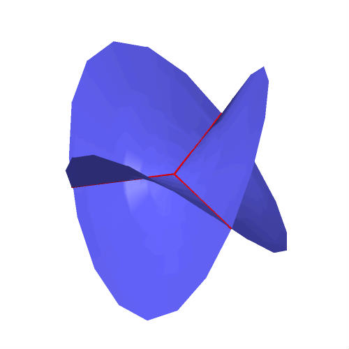
Figure 4.1.1. The front projection of near a vertex. - (2)
A period domain , which is an algebraic torus equipped with an algebraic symplectic form coming from the intersection pairing on [TZ, §4.6]. More precisely, let be the set of branch points of , corresponding to the vertices of . The period domain is the moduli space that parametrizes flat line bundles over such that the monodromies surrounding the branch points are Note that can be identified with the moduli space of flat line bundles over . It acts on by taking the tensor product of corresponding line bundles, and this action equips with the structure of an torsor.
- (3)
A moduli space of microlocal-rank-one constructible sheaves on , whose singular support lies in [TZ, §4.3]. More concretely, is the space of -equivalence classes of -colorings of the faces of .
- (4)
A Lagrangian microlocal monodromy map [TZ, §4.7]. It can be described as follows. Every edge of connects branch points and therefore defines an element of It gives rise to a character by the canonical pairing between and . The sum of edges surrounding a face is a trivial cycle in , so The map is defined by setting to be the cross ratio
(4.1.1) where are the colors of faces surrounding an edge in the following pattern:
One easily verifies the relations .
We exhibit defining equations for The characters generate the coordinate ring of , obeying the relation
(4.1.2) and further the equation
(4.1.3) whenever label the edges of a face of . In these coordinates, the map is given parametrically by the cross ratio (4.1.1). But it is also given by equations, as a complete intersection, in the following way. Let be the set of faces of . If are the edges around a face taken counterclockwise, then the expression
(4.1.4) is independent of which edge is called . is cut out by the equations .
Now let denote the dual planar graph, with vertex set . Since is cubic, is a triangulation of , and we regard its vertices as punctures on the sphere in the sense of Section 2.4. Now let be a sphere with punctures, and recall the corresponding moduli space of decorated local systems on .
Theorem 4.1.
Let be the symplectic subvariety of the cluster Poisson moduli space cut out by equations (4.1.3). There is a canonical algebraic Lagrangian subvariety with the following property: for every cubic planar graph with vertices, there is a cluster chart such that the embedding is isomorphic to .
Proof.
The subvariety is given by the subvariety of decorated local systems whose underlying local system is trivial. We show that the intersection of with coincides with using the prescription for constructing a decorated local system corresponding to a point in a cluster torus described in Section 9.10 of [FG1].
Let be the torus parametrized by the edges of the triangulation . As in Corollary 9.1 of loc.cit., there is an open torus embedding
The image of together with the variables parametrized by the edges of give rise to a cluster seed of .
In more detail, let be as in (4.1.1). Without loss of generality, assume that . The cross ratio implies that . The Möbius transformation taking the triple to corresponds to
The punctures on the sphere correspond to the vertices of , or equivalently, to the faces of . Let be the variables associated with the edges of surrounding a vertex . Under the map , the holonomy surrounding the vertex is
| (4.1.5) |
where is given by the expression (4.1.4).
By the expression (4.1.5), the conditions (4.1.3) generate the defining ideal of the intersection of the unipotent subvariety with the image of . The triviality of the holonomy of the underlying unipotent local system around such a puncture is equivalent to the vanishing of the corresponding expression (4.1.4).
Remark 4.2.
Because of item (3) above, we refer to as the chromatic Lagrangian. The definition of from a dual perspective, along with its Lagrangian nature, were initially established in the earlier work of Dimofte-Gabella-Goncharov [DGGo]. In this paper, our equations (4.1.3) provide an explicit description of for every cubic planar graph . This presentation is novel and crucial for the quantization of , as discussed in Section 4.3. Meanwhile, our proof of the Lagrangian property of via the involution in Section 2.5 is new and relatively simple, which can be generalized to the setting of any semisimple group.
4.2. Mutation and quantization
We define a Poisson torus. It has a canonical quantization , generated by coordinates with relations
| (4.2.1) |
Let be a framed seed with underlying cubic graph , and let be the graph obtained from by flipping a single edge . Then the positive and negative lattive mutation maps deliver isometries of edge lattices , and so define framed seeds . The corresponding isometries of lattices are illustrated below:
| (4.2.2) |
Also associated to each flip of triangulation is a cluster transformation, i.e. a birational map of tori As explained in Section 2, these maps admit quantizations , which in our case take the form
| (4.2.3) |
The map can be factored in one of two ways, corresponding to the choice of sign in the lattice isomorphism . Indeed, one easily verifies that the quantum cluster transformation corresponding to the flip at edge can be written as
Now consider a morphism in the framed seed groupoid represented by a sequence of signed edge mutations :
where the th mutation takes place at edge and has sign . It gives rise to an isomorphism of quantum tori given by
Moreover, if we write for the image in of the quantum torus element under the isomorphism
then we have
Per Equation 3.1.3, such a sequence of mutations of framed seeds gives rise to a birational automorphism of , which evidently factors as
where we have set
The reader may find it convenient to visualize the automorphism as follows. Recall that the data of a framing for a seed gives rise to a decoration of the edges of its cubic graph by monomials . Then the automorphism is characterized by the property that it maps the monomial sitting on edge of in framed seed to the monomial sitting on the corresponding edge of in framed seed .
Now let us suppose that each signed mutation in the sequence is admissible, so that under the framing isomorphism from the monomial is mapped to an element of the algebra . Then we may form the product
Recall the representation of the algebra . The action of defines an automorphism
and for all , we have the following identity of operators on :
| (4.2.4) |
In particular, if and are related by , then we have
| (4.2.5) |
as operators on .
The torus associated to a cubic graph , or its quantization , is the cluster chart of described in Sections 4.1. In the next section we show that the global Lagrangian submanifold is compatible with this chart-wise quantization.
4.3. Quantizing the Chromatic Lagrangian
We begin by discussing the quantization of the relevant connected component of the moduli space of framed local systems with unipotent monodromy on the punctured sphere. Fix a cubic graph of genus , and as in the previous section let be the associated quantum torus. Suppose that are the edges around a face of , listed in counterclockwise cyclic order around the face; note that this means that each precedes in the counterclockwise order with respect to their common vertex, so that we have
Then the relation (4.1.3), which imposes unipotency of the monodromy around the puncture dual to the face , is quantized as
| (4.3.1) |
Note that the relation 4.3.1 can be equivalently formulated as In order to pick out the required component, let be the sum of the edges. We then further impose the relation that
| (4.3.2) |
After quotienting by these relations, we obtain a symplectic quantum torus algebra .
We now proceed to the quantization of the additive face relations that are equivalent to the triviality of the underlying unipotent local system at a point of . To this end, set
| (4.3.3) | ||||
Remark 4.3.
Let be the left ideal in generated by all (4.3.1) along the global relation (4.3.2) and the relations for all faces . As the quantization of a Lagrangian subvariety, the D-module is holonomic.
Now suppose that two regular cubic graphs and are related by mutation at edge . Let us write for the localization of the quantum torus at the Ore set , and write for the analogous localization of . Then the quantum mutation map in (4.2.3) defines an isomorphism . Let us write for the ideal in generated by the quantized chromatic ideal , and for the ideal in generated by .
Theorem 4.4.
The system of quantized chromatic ideals is compatible with quantum cluster mutations: if are regular cubic graphs related by a flip at edge as in Figure 4.2.3, then we have .
Proof.
Consider the generator of associated to the left face of the graph in Figure 4.2.3, as defined in (4.3.3). We show that it is mapped to the corresponding to a generator of under . As explained in Remark 4.3, by multiplying by a unit in we may assume that the edge at which we mutate is neither nor in the notations of (4.3.3). Then reading counterclockwise around the left face of the right graph in Figure 4.2.3, we see that
where we used that by the relation (4.2.1) applied to the graph on the left of Figure 4.2.3. From this computation, we see that . The intertwining of the generators of the form (4.3.1) and (4.3.2) follows in exactly the same way. ∎
Remark 4.5.
In this lengthy remark we explain the sense in which Theorem 4.4 allows us to build a global quantum Lagrangian from the compatible system of ideals in the different cluster charts. In this context, Theorem 4.4 implies the Lagrangian has a well-defined ‘quantum structure sheaf’, which is an object in the category of representations of the quantum cluster variety . The category of such representations can be defined by means of the gluing procedure explained in [BBP]. Indeed, let us fix as in Section 2.2 an initial seed with corresponding basis for the lattice . As in that section, we write for the set of all bases for reachable from by some sequence of sign-coherent mutations. For each we take a separate copy of the same abelian category of left modules over the quantum torus algebra associated to the lattice , and form the category .
As explained in 2.2, for each we have an element that depends only on the basis and not the mutation sequence leading from to it. Given a pair we set
We use these elements to define -bimodules . When correspond to cubic graphs differing by a single mutation, this bimodule is the one coming from the ring defined earlier by Ore localization. Tensoring with any bimodule defines an endofunctor on , and together they form the components of an endofunctor . The maps coming from the inclusions
define a natural transformation making into a comonad. The category of representations of the quantum cluster variety can then be defined as the category of comodules for this comonad. Objects of this category are objects of together with a morphism satisfying and , where is the counit transformation projecting to the diagonal components.
The object where each and the map is defined by the inclusions
| (4.3.4) |
plays the role of the structure sheaf of the quantum cluster variety. Its endomorphism ring is naturally identified with the algebra of universally Laurent elements in . So we have a global sections functor
In concrete terms, a global section of is described by a collection of elements satisfying . The global sections functor has a left adjoint which sends a module over to its localization, i.e. the object of with components .
Now suppose we are given a collection of left ideals satisfying
for all . Setting , this condition implies that the maps in (4.3.4) descend to maps , and we get an object of . So in this language, Theorem 4.4 implies that the system of ideals defines a representation of the quantum cluster variety . In particular, taking global sections of this object defines a global chromatic left ideal .
A similar construction can be performed using the admissible framed seed groupoid , where we replace by the quantum torus , and the elements by the ones associated the to arrows in , as defined in Section 3.4.
We now illustrate the constructions of this section in the following simple but fundamental example.
Example 4.6.
Consider the framed seed for the necklace graph shown in Figure 4.3.2. The additive face relation
corresponding to its left bead is mapped under the corresponding framing isomorphism to the element
Let us now perform a positive mutation at the edge of to obtain the framed seed for the canoe graph shown in Figure 4.3.2. Then we see that
where is the additive face relation associated to the face of bounded by . Under the new framing isomorphism , the element is mapped to
| (4.3.5) |
The element is given by
and hence the operators associated to the face relations are indeed intertwined under by the action of : we have
5. Foams, Phases and Framings
We have shown that the moduli space of constructible sheaves with singular support on a Legendrian surface is a (quantum) Lagrangian subvariety (ideal) of a symplectic leaf in a (quantized) cluster Poisson variety. This ideal is defined by a “wavefunction.” The purpose of this section is to describe the combinatorics of non-exact Lagrangian fillings of the Legendrian. The geometric/combinatoric set-up will allow us to make conjectures about open Gromov-Witten invariants of the pair
Here are the constructions we describe. We begin with a Legendrian surface defined by a cubic planar graph as described in previous sections.
- •
A singular exact Lagrangian filling is constructed from an ideal foam,
- •
A deformed foam determines a non-exact Lagrangian filling, .
- •
is a branched double cover of the three-ball, branched over a tangle, also defined by
- •
A deformation is described by a short arc between strands of the tangle at each vertex.
- •
The map is determined combinatorially from and the arcs.
- •
A splitting of the map gives a phase and framing.
- •
We further require a maximal cone of
- •
These constructions allow us to make open Gromov-Witten predictions about
- •
All these notions can be carried through allowed mutations of the deformed foam
The upshot is that we get open Gromov-Witten predictions from the wavefunction at all points of the framed seed groupoid accessed by allowed mutations from the necklace foam. This is a large class of Lagrangian fillings and framings.
We now proceed as outlined above.
5.1. Foams
A cubic graph on the sphere is dual to a triangulation of . If is three-connected, then by Steinitz’s theorem it is the edge graph of a polyhedron. A foam is the dual structure to a tetrahedronization of the polyhedron: it is a polyhedral decompsition of the three-ball with The data of includes the quadruple of regions, faces, edges and vertices. A face or edge is called external if it intersects the boundary, and internal if it does not. The foam is ideal if it is dual to an ideal tetrahedronization of , i.e one with no internal vertices. Even if is not dual to a polyhedron, the notion of ideal foam makes sense — see [TZ, Definition 3.1]. For example, if there is a bigon between two vertices, then there is a single edge of the foam whose boundary is those vertices — see Example 5.1.
Example 5.1 (Foam filling for ).
The necklace graph has a distinguished foam filling, that we in fact believe to be unique. This foam has no vertices: is already smooth — in other words there is a unique phase. See Figure 5.1.1 below. In fact, using the local construction at the left of Figure 5.1.1, we can construct similar foam fillings of any iterated sequence of bigon additions (handle attachments for the Legendrian surface), starting from the genus-zero necklace (theta graph). We refer to these as necklace-type graphs, and equip them with these canonical foam fillings. Note that while generic foams are dual to tetrahedronizations, these foams are dual to somewhat degenerate tetrahedronizations. For that reason, we will mainly focus on foams and not their duals.

5.1.1. The Harvey-Lawson Foam
The foam of the Harvey-Lawson Lagrangian has a single vertex at the origin in four edges equal to the rays where and , with the standard basis vectors. There are faces equal to the cones spanned by unordered pairs of edges, and regions equal to the cones spanned by triples of edges. (It can be succinctly described as the toric fan of )
The singular, exact Harvey-Lawson Lagrangian in is a branched cover of branched over the over edges. is a cone over with parametrization , where and The covering map is the restriction to of sending a complex triple to its real part: explicitly The map is over the four rays with which we think of as a singular tangle. The six sheets of the foam are defined by
The primitive function obeying is Note that is odd under the hyperelliptic-type involution and along the preimages of the sheets of the foam. Thus allows us to label the branches of on the regions .


5.1.2. Foams and singular exact Lagrangians
From a foam we can define a singular exact (not necessarily special) Lagrangian locally modeled on the Harvey-Lawson cone and foam — see [TZ, Section 3.2]. As with the Harvey-Lawson cone and foam, we can define a multi-valued function whose sign labels the branches of in the regions of the foam.
5.1.3. Deformation of the Harvey-Lawson foam
There are three distinct families of smoothings of corresponding to the three matchings of the four edges. We will describe the one for the matching ; the others are similar and are related by a permutation of coordinates. The smoothing has the topology of and has a parametrization in polar coordinates , which maps to These are all diffeomorphic for so when we are interested in topological questions, we can restrict to without loss of generality. The branched cover is over the points with and these parametrize four rays which trace out two hyperbola components ( and ), a smoothing of the singular tangle of . )
There is also the line segment between and which we call an arc — it is the image of Note that is over the arc. The six sheets now bound either a smooth edge if or , or otherwise the union . This will be our local model of a deformed foam. More generally, let be the matching of edges of which pairs and . We write for the local deformed foam of Its arc is the line segment between and . We write for the deformed foam of
Away from the origin and the preimage of the arc, the Harvey-Lawson cone and its smoothing are homeomorphic: . As a result, the same primitive function can be used to label regions of the foam and of its deformation, at least away from the arc. The local geometry of and the deformed foam near an arc is shown in Figure 5.1.4.
5.1.4. Deformed Foams
Given a foam , we will define a deformed foam to be a structure locally modeled near each vertex on a Harvey-Lawson deformed foam.
Definition 5.2.
Let be a foam with vertex set consisting of vertices. Write for the set of matchings of half edges at each vertex, so Let . We define a deformed foam to be any set of vertices, edges, arcs, faces and regions which agrees with outside some -neighborhood of , is homeomorphic to outside of a -neighborhood of , and which is linearly equivalent to the local deformed foam of of Section 5.1.3 within a -ball of each vertex.
The smoothed Lagrangian is branched over a tangle i.e. is a one-manifold. The construction of from a deformed foam identities a particular set of branch cuts we call arcs.
Definition 5.3.
Let be the smoothing of the Harvey-Lawson foam which matches the ray with , where and are as in Section 5.1.1. The arc of the deformed Harvey-Lawson foam is the line segment from to . An arc of a deformed foam is the locus in corresponding to the arc of the Harvey-Lawson foam under the local identification of with . We write for the set of arcs of a deformed foam .
Given an arc of a deformed foam and its associated branched double cover define Since is over the interior of the arc and at its edges, is a circle. Note that does not (yet) have a distinguished orientation.
Remark 5.4.
If is a foam, a deformed foam is defined by choosing a matching of the four internal edges meeting at each vertex. In the case of the necklace graph , the foam has no internal vertices, and therefore . In particular, is already deformed. In fact, we will learn that the strands of can be thought of as the arcs of , and the face of which they bound gives rise to a single relation among them – see Definition 5.12 and Proposition 5.13. Similar considerations apply whenever has a bigon.
5.2. Phases and Framings
Definition 5.5.
Let be a rank- lattice with a non-degenerate, antisymmetric pairing A phase is a rank- isotropic subgroup . A framing of is a transverse isotropic subspace. We call the combination of phase and framing an isotropic splitting, or sometimes just splitting.
We will be studying phases and framings when is the homology of a genus- surface, and is the intersection pairing. So let be an orientable three-manifold with boundary a genus- surface , with . Then it follows from the long exact sequence in homology together with the Poincaré-Lefschetz duality isomorphisms that 33 3 In this section, homology will be taken with coefficients unless otherwise stated. so that we obtain the short exact sequence
| (5.2.1) |
The notion of phases and framings will apply to above geometic setting.
Definition 5.6.
In the context of open Gromov-Witten theory, is Legendrian in a contact manifold and is Lagrangian in a symplectic filling.
Remark 5.7.
In [TZ], the above geometric phases were called “OGW framings” to connote open Gromov-Witten theory. The definition was generalized from [AKV], where mirror symmetry was used to make conjectures in open Gromov-Witten theory.44 4 In [I] a similar definition of framing is made, but without the isotropic condition. The terminology stems from the connection to Chern-Simons theory through large-N duality, where Lagrangians are knot conormals and framing relates to the framing of knots. We describe the connection to open Gromov-Witten theory later in this section.
Remark 5.8.
We need phases and framings to define a framed seed as in Definition 3.1, from which we will construct wavefunctions and conjectural enumerative inormation — see Conjecture 6.9. The geometry behind this is as follows. Let be the cluster variety of framed local systems on a sphere. Let be the symplectic leaf of unipotents, and let be the Lagrangian subvariety defined by trivial monodromy. Let be a cubic graph on the sphere and the associated a Legendrian surface up to isotopy. We write for the corresponding cluster chart.55 5 As explained in Section 4.1, the cluster charts of are spaces of rank-one local systems with fixed monodromy around the critical points of the branched double cover Since is a torsor over , its tangent space at any point is canonically and its Poisson structure is determined by the intersection form on independent of choice of base point. Hereafter, we often omit the distinction and refer to cluster charts as the tori A splitting allows us to write as . When we lift to we can write it locally as the graph of the differential of a function on , from which we will extract enumerative information — see Section 8.5.
Recall from [TZ] the combinatorial model of the first homology of a Legendrian defined from a cubic planar graph on a sphere, . The faces of define a relation on the edge lattice , namely We then have . We have an antisymmetric pairing on , depending only on the orientation of , defined by if and are adjacent to a vertex with preceding/following in the cyclic ordering at the vertex , and zero otherwise. Since generates the kernel of this pairing, descends to a nondegenerate, antisymmetric intersection pairing on
| (5.2.2) |
We now have a combinatorial model of We next build combinatorial models of for arising from a deformed foam, and of the map
5.3. Combinatorics of Tangles from Deformed Foams
We continue our study of smooth Lagrangians arising from deformed foams. Cutting to the chase, the loops defined by the edge set and arc set will generate and , with relations determined by faces. In total, we find
Here is induced by the inclusion and the top line was defined in the previous section. The bottom line will be defined in this section.
Let be a cubic graph on the sphere, let be an ideal foam on the three-ball , whose regions, faces and edges respectively bound the faces, edges and vertices of . Let be the discrete set of smoothings of , i.e. the set of matchings of edges incident to each vertex of — so Let be a smoothing whose resulting tangle has no circle components. Let be a smooth Lagrangian corresponding to the deformed foam .
Recall that for an arc we werite We now define an orientation on , thus definining an element
Since the construction of the smoothing is local, we need only look at the Harvey-Lawson smoothing and its unique arc , which we can lift to the parametrized curve and take the induced orientation. This is the orientation induced from the unique holomorphic disk in bounding , i.e. We can also give a more combinatorial construction that does not require an explicit local model, as follows.
Definition 5.9.
We choose a canonical orientation for by orienting the arc arbitrarily and taking a push-off of the path along the arc that has some combinatorial properties, using the primitive function, . We require that near the start of the push-off, in the chosen orientation, that has a negative value and lies in one of the two fat regions (see Figure 5.1.4) — in particular, outside of two sheets which meet at the arc’s origin — then crosses once at the midpoint of the arc in a counterclockwise direction (in the induced orientation of the transverse plane). The remainder of traverses the arc backwards after crossing the origin of the transverse plane at the arc’s endpoint, and has the same combinatorial recipe as the first half of This completes the description of the push-off, There are actually two such push-offs, but the resulting paths are homotopic. Likewise, the opposite orientation of the arc leads to a homotopic path (just shifted). For an arc , write for the resulting element of
Remark 5.10.
For each face of the deformed foam we will define a relation among the edges and arc loops along its boundary. Together these relations will characterize as To define the relation, we need a careful discussion of the sign of an arc relative to a face.
Definition 5.11.
Let be a face of a deformed foam bounding an arc . Then we have a homeomorphism of a neighborhood of with a neighborhood of the lone arc of the Harvey-Lawson deformed foam defined by some smoothing which pairs the edges containing vectors and — see Section 5.1.3. Let be the face of corresponding to , which deforms the face of containing and (note ). Let us orient the arc from the end bounding the strand of the tangle deforming the edge of with to the end bounding the tangle strand deforming the edge with . Call a vector along the arc in this orientation . We define the sign of the arc relative to the face by
Note that the opposite orientation on the arc leads to which is the same. The definition therefore only depends on the orientation of .
Definition 5.12.
Let be foam with boundary and let be a deformed foam with arc set . We define a relation on by setting
| (5.3.1) |
for each face of .
5.4. Face relations for foams
On general grounds, with and defines a phase as the kernel of the surjection Here we want to understand this combinatorially when arises from a deformed foam , in terms of its arcs and the edges of
Proposition 5.13.
Let be an ideal foam filling a cubic graph with edge set , and let be a smoothing associated to a deformed foam with arc set , such that the corresponding tangle has no circle components. Let be as in Definition 5.12. Then , and we have an isomorphism
such that the homology pushforward is identified with the map induced by the inclusion .
Before the proof, a remark.
Remark 5.14.
If has no bigons, then each edge is equivalent to a sum of arcs under Equation 5.3.1 by the external face of containing in its boundary. Then after taking the partial quotient of by the external faces of , we may think of as
Proof.
We prove the proposition by induction on the number of internal vertices of a foam
The base cases (no internal vertices) then consist of any of the canonical foam filling of necklace-type graphs of any genus, as in Example 5.1. Each such graph is itself obtained from the genus- necklace (theta graph) by bigon addition, or Legendrian one-handle attachment of the corresponding Legendrian surface — see [CZ, Theorem 4.10(1)]) — so we treat the base cases themselves by induction on the genus. The genus- foam consists of the three filled semicircles in the unit ball at azimuthal angles The edge lattice modulo face relations is zero, as is for the filling, and the proposition is true. Now we induct on the genus of the base case by adding bigons. Each bigon addition adds three edges and one face to the boundary, as seen here,
thereby increasing of the Legendrian by and the genus by . Two faces are added to the foam, which end in the two edges of the bigon. The bigon edges sum to zero in homology of the Legendrian, by the relation from the bigon face. The foam face relations then show that these edges are trivial in of the filling, thus in the kernel of the homology map corresponding to inclusion of the boundary — see Figure 5.1.1. The difference is in no boundary and therefore is an additional nontrivial class in of the Lagrangian filling the new Legendrian. This establishes the base case of no internal vertices, for every genus.
We now induct on the number of internal vertices by attaching a Harvey-Lawson foam. We can attach at a single vertex, along an edge, or a face. To verify the inductive step in the first case, let be a smoothed ideal foam, whose boundary is a cubic graph of genus .
Now suppose is a single tetrahedron together with a smoothed Harvey-Lawson foam in it. Let us choose a vertex of along with a vertex of the cubic graph on the boundary of the tetrahedron. Let us write for the three edges of incident to the vertex listed in cyclic order determined by the orientation, and similarly write for the edges of incident to , but listed in opposite cyclic order. Each of these edges determines an external face of the corresponding foam, which we denote by or . We glue a neighborhood of the vertex to by identifying the tetrahedron (dual) face corresponding to with the boundary (dual) face of corresponding to as indicated in Figure 5.4.1, so that each edge is glued to the corresponding to form a new edge . As a result of this gluing, we obtain a new ideal foam .
The set of faces of the new deformed foam may be described as follows. The internal faces of are the same as those of . The set of external faces of consists of all those external faces of and that correspond to edges of or not incident to , along with three faces obtained by gluing each to the corresponding .
We now turn our attention to the effect of this gluing at the level of the double covers of the ball. Let us write , for the branched double covers corresponding to and respectively, so that we have , where is the neighborhood of the vertex where we attached , i.e. the face of along which the dual tetrahedron was glued. This gluing is illustrated in Figure 5.4.2.
Now since the space is homeomorphic to a disk, the Mayer-Vietoris long exact sequence shows that . Similarly, it delivers an isomorphism
| (5.4.1) |
such that . Hence all that remains is to verify the face relations for the faces of obtained by gluing faces of to those of . But recall from 5.11 that the definition of the sign of an arc relative to a face is entirely local, depending only on the tangent vectors to the two edges of the deformed foam that meet and bound . So if is the unique arc at the vertex of that is connected to by an edge, and the corresponding arc in (connected to ), the sign of with respect to face in is identical to its sign with respect to face of the glued foam . Similarly, the sign of with respect to coincides with its sign with respect to . The face relation for is therefore obtained as the sum of those for and under the isomorphism (5.4.1).
We next consider the case of gluing in a Harvey-Lawson cone along an edge. We have a foam with boundary and a Harvey-Lawson foam with boundary a tetrahedron graph Suppose that we fix an edge of connecting two vertices , and correspondingly fix an edge of connecting vertices of . Let us denote the edges of incident to by , cyclically ordered in accordance with the orientation of , and similarly write for the edges incident to . We denote by the edges incident to but ordered with respect to the opposite of the orientation on , and similarly write . We write for the remaining edge of which is incident to neither nor . We now glue the foam to by identifying the edges so that each edge is glued to the corresponding . We denote by the ideal foam produced as a result of this gluing.
Note that the cubic graphs and have the same genus: indeed, the two are related by a single diagonal exchange/edge mutation, as illustrated in Figure 5.4.3. (We will return to this point in Proposition 5.22.) The set of external faces of is thus in natural bijection with that of : the latter contains the external faces obtained by gluing each face to the corresponding , along with the external face with boundary . On the other hand, we now have a new internal face created by gluing to . By assumption, the smoothing of the foam in is chosen such that the tangle in the glued deformed foam has no circle components; this is equivalent to requiring that at least one of the faces contains an arc as part of its boundary.
We now consider the gluing of double covers and . We have , where is a neighborhood in of the edge , or dually the quadrilateral along which the dual tetrahedron is glued to . As shown in Figure 5.4.4 the space is homeomorphic to a cylinder . We fix the isomorphism , where we take the generator to be the oriented loop on given by canonical lift of the edge of . The relevant part of Mayer-Vietoris sequence then reads
| (5.4.2) |
By our assumption that at least one of the faces contains an arc as part of its boundary, we see that the map
is injective. Hence , and
The face relations for all external faces of now follow from this description of exactly as in the case of the single-triangle gluing. Finally, since
we see from the isomorphism (5.4.2) that the relation in corresponding to the new internal face is also obtained as the sum of the relation corresponding to in with that corresponding to in .
It remains to consider attaching along a triangular face. The proof is very similar to the above case, so we only comment briefly. In this case, the attachment is along a punctured torus, so has rank two. It still injects into , and otherwise the exact sequence looks the same. Therefore has rank one less than . The rest of the proof is as above.
This completes the proof of the Proposition.
∎
5.5. Example – triangular prism
Let be the edge graph of a triangular prism and let be the deformed foam pictured here:
Write for the gray face and for the pink face. Then and from Equation 5.12, gives the relation
In total, the external face relations give
We also have the internal (gray) face relation, and since we see
The relations are consistent with the face relations from . For example, the sum , and this implies or and this is true by the internal gray face relation of . The other face relations are consistent, as well.
So indeed descends from a map from to one from giving a map to . is rank- and we can take Darboux generators (careful about the cyclic order on the back side of the prism: ). is rank- and we can take generators . With these generators,
We can see that the kernel of is generated by and and is indeed isotropic. A framing must send to and to The image is isotropic if so the different framings for this phase are parametrized by symmetric integer matrices
5.6. Associated Cones, Geometric Cones
To formulate open Gromov-Witten conjectures, we want to express a wavefunction in a power series about a limit point of the moduli space. A phase and framing define an algebraic torus, but pinning down a limit point for the expansion requires the notion of an associated cone, which we define below after setting notation.
We write for the underlying cubic graph, for the associated Legendrian surface, for the deformed foam, and for the corresponding Lagrangian.
Definition 5.15.
Given a splitting, i.e. a phase ) and a framing -isotropic and transverse to (so ), an associated cone (or just cone) is an open integral convex cone containing no lines.
With Remark 5.14 in mind, if is simple (in particular has no bigons) and we are given a splitting, then we can specify an associated cone by choosing a spanning set of arcs.
Definition 5.16.
Define a geometric cone of a deformed foam with to be the span of a spanning set of arcs and edges in When is simple, without loss of generality we take a spanning set of arcs.
Example 5.17.
Let be the foam for the necklace graph (see Remark 5.4), and the corresponding Lagrangian. Label the beads through in clockwise order from some chosen starting point, and let , be edges along the outer edges of the corresponding bead. Label the strands of the necklace , so that the th strand succeeds the th bead in clockwise order and The span the kernel of , so define a phase. (The strands function as arcs, albeit there are no vertices, as they connect tangle components.) The map defines a splitting We note the following relations in : So any -element subset of determines a geometric cone, and by symmetry we may as well take this to be The necklace therefore has a unique (up to symmetry) phase, framing and geometric cone.
Example 5.18.
A Harvey-Lawson smoothing has a single arc and therefore a unique geometric cone. The blue edges are equivalent under the face relations and span the kernel (phase) of A splitting is defined by mapping the green arc to a transverse element of and the unique associated cone is the span of this vector.
5.7. Mutations of Foams and Cones
We now show that for a large class of mutations of the boundary graph, the foam filling can be mutated, along with a phase, framing and cone.
Definition 5.20.
A mutation of a deformed foam at an edge is allowable if is not the boundary of a single tangle strand.
The reason for this definition is to exclude the case where the class is in the kernel of , rendering the action on the wavefunction zero. At the level of tangles, the condition ensures that the new tangle has no circle component.
Proposition 5.21.
Let be a cubic planar graph bounding a deformed foam . Let be the graph defined by performing an allowable mutation at the edge . Then there is either one or two canonically defined deformed foams and with boundary corresponding to positive and negative mutations, respectively.
Proof.
The proposition follows immediately from the proof of Proposition 5.13: the allowed mutations correspond to attaching a Harvey-Lawson foam along an edge, with the allowable condition corresponding to the hypothesis that the tangle of the deformed foam have no circle components. Nevertheless, for the convenience of the reader, we provide a separate description in the language of triangulations — though they are not as general as foams (the foams of necklace-type graphs are degenerate tetrahedronizations), they are often easier to visualize.
We first mutate the ideal foam , then worry about its deformation . On the surface the geometry near the dual edge of is a quadrilateral as pictured here:
Define as follows: if the two faces above are part of a tetrahedron , then Otherwise, let be the tetrahedron with two faces as pictured above and the other two and , and set In both cases, the geometry of the quadrilateral at the boundary of is
Call the foam so constructed . It remains to describe how to deform to
Suppose is formed from by adding a tetrahedron as in the proof of Proposition 5.13, and so is formed from by attaching a Harvey-Lawson foam . We define by extending together with a choice of one of the three possible smoothings of One of these three pairs the two tangles with endpoints at the centers of triangles and (pictured in red and blue) with one another, creating a new short tangle component. This is the disallowed smoothing. The other two rotate pair these with the centers of the two new triangles and . The matching corresponding to the deformed foam of the positive mutation is shown above. is defined similarly.
Now suppose otherwise that is formed from by deleting a tetrahedron . Then was the result of a mutation of and only the inverse mutation is possible. Since the case where bounds a single tangle component is not allowed, the tangle components after deleting the tetrahedron are clear: they are truncations of the original tangle strands.
∎
Proposition 5.21 will allow us to transport foams across mutations, along with phases, framings and cones. This will allow us to connect open Gromov-Witten conjectures for Lagrangian fillings related by allowed mutations which have corresponding cones, phases and framings.
Proposition 5.22.
Let and be deformed foams corresponding to an allowed mutation of their boundaries. Then there is a canonical isomorphism
Proof.
We can assume that is obtained by attaching a tetrahedron, as removal will give rise to the inverse isomorphism. A local study near the attachment will suffice to establish We label the relevant edges and vertices as in the figure below, with indicated by dashed lines.
Consider the sheets of the deformed Harvey-Lawson foam, after gluing to and deforming. They correspond to unordered pairs from among the vertices . Write for the face determined by and , and likewise for the others. Let be the arc of the Harvey-Lawson deformed foam, and write for the signed contribution to the relation from , as defined in Definition 5.12. Now suppose the face relations on relate give , , and so on. Let us list the unordered pairs along with the relations from the corresponding glued face.
This gives the positive mutation. The other allowed matching gives the negative mutation, as follows from the interchange
∎
Corollary 5.23.
Proof.
It only remains to note that respects the antisymmetric pairing of edges. ∎
We immediately obtain the following.
Corollary 5.24.
The maps and map phases, framings and cones to phases, framings and cones.
6. The wavefunction
6.1. Construction of the wavefunction
Suppose that is a deformed ideal foam obtained from the standard necklace foam by a sequence of admissible mutations, and is a framing for . As explained in Section 5, the pair gives rise to a framed seed . It is convenient to visualize the framed seed as a labelling of the edges of the cubic graph by monomials in the standard quantum torus generated over by .
In this section, we will show that there is a canonical wavefunction associated to such a framed seed, thereby providing a prediction for the generating function of all-genus open Gromov-Witten invariants of the corresponding Lagrangian .
We begin with the definition of in the case of the standard necklace framed seed . The corresponding foam gives rise to an exact Lagrangian filling of the Chekanov surface, so that by Stokes’ theorem all its open Gromov-Witten invariants will be zero. We therefore take the wavefunction for the standard necklace to be . Let us note that the necklace wavefunction depends only on the underlying deformed foam, and is completely independent of the choice of framing .
Now recall the sub-category of the framed seed groupoid whose morphisms are given by the admissible ones, and let be the connected component of containing the framed seed .
Part of the data of a representation of a quantum cluster variety (as defined in [FG2]) consists of a functor from the cluster modular groupoid to the category whose objects are Hilbert spaces, and whose morphisms are unitary equivalences.
By analogy, let us define an algebraic representation of the admissible groupoid to be a functor from to the category of -vector spaces with morphisms given by -linear maps.
The results established so far allow us to construct an algebraic representation of as follows. Consider the functor which assigns to each object of the same vector space , and assigns to each arrow in the automorphism of defined in Section 3.4. In this language, Lemma 3.6 implies
Lemma 6.1.
The assignment
defines an algebraic representation of the admissible groupoid .
For each object of , we now explain how to construct a canonical vector which we call the wavefunction of the framed seed . This vector is constructed as follows: choose an arbitrary path in . By Lemma 6.1, the morphism gives rise to an automorphism of , which we apply to to produce a candidate for :
| (6.1.1) |
What must be checked in order for this definition to make sense is that the wavefunction depends only on the endpoint of the path in the framed seeds groupoid. This path-independence is the content of the following Theorem.
Theorem 6.2.
Proof.
The key observation is the following immediate consequence of Theorem 4.4: if satisfies the face relations in framed seed and where is an admissible mutation or framing shift, then satisfies the face relations for . Now suppose we have two sequences of admissible mutations and framing shifts and as in the statement of the theorem. Then it suffices to show that
| (6.1.2) |
To this end, consider the framed seed . Its underlying cubic graph is the image of the original necklace graph under an element of the mapping class group of the -times punctured sphere, and moreover the labelling of the edges of by monomials in the induced by its phase and framing are identical to that in the standard necklace framed seed. In particular, the face relations for and are identical, and from the binomial face relations corresponding to the beads we deduce that
It follows that , which completes the proof that the map is well-defined. The Ooguri-Vafa integrality follows from Proposition 6.15, which is established in Section 6.4. ∎
6.2. Examples of wavefunctions
We now proceed to compute the wavefunction defined in the previous section in some fundamental examples.
Example 6.3.
The calculation in Example 4.6 shows that the wavefunction associated to the framed seed for the canoe graph shown in Figure 4.3.2 is given by
It satisfies the -difference equation
which is a scalar multiple of the face relation in (4.3.5). As an exercise, let us compute the effect on the wavefunction of applying the framing shift operator , which we recall acts on by . The resulting framed seed is illustrated in Figure 6.2.2.
Lemma 6.4.
We have
| (6.2.1) | ||||
Proof.
Since
the Lemma follows by observing that both sides satisfy the -difference equation
which is easily seen to have a unique formal power series solution of the form . ∎
Now observe that applying to the framed seed the positive mutation at edge 4 returns us to the framed seed shown in Figure 6.2.2, which coincides with the standard necklace up to a permutation of the numbering of its edges. Hence we have a loop in the framed seed groupoid
| (6.2.2) |
and we indeed see that
in accordance with Theorem 6.2.
More generally, we can consider the framed seed obtained from the standard genus necklace framed seed by performing positive mutations at all beads labelled under the framing isomorphism. The corresponding wavefunction is then
| (6.2.3) |
which is annihilated by the left ideal in generated by
| (6.2.4) |
Let us write for the wavefunction obtained by applying the operator to , where is the identity matrix. Then we again have
| (6.2.5) |
Lemma 6.5.
The explicit power series of the wavefunction (6.2.5) is
Proof.
Set
Let be the unit vector. At the level of the coefficients of , the equation is equivalent to the recurrence
Note that . Therefore we have
∎
More generally, given a integer symmetric matrix , let us consider the framed seed obtained by applying to . Then by (3.3.2) we have
| (6.2.6) |
Example 6.6 (Non-existence of algebraic wavefunctions).
Algebraic wavefunctions may not exist for framed seeds which cannot be obtained from the standard necklace by a sequence of admissible mutations. A simple counterexample is given by the framed seed obtained from the standard necklace by performing positive mutations at both of its strands to produce another necklace graph. The arguments of the corresponding quantum dilogarithms are and , only the first of which corresponds to an admissible mutation. The face relation associated to the bead of the resulting framed seed imposes the difference equation , and it is easy to see this admits no nonzero solutions in the ring (or for that matter in the opposite completion .
We conclude this section with an example from [AENV] concerning the unknot conormal after the conifold transition.
Example 6.7 (Partition function for unknot conormal [AENV]).
Set
where the closed-string parameter is a formal variable commuting with all the other variables. Then is annihilated by
Lemma 6.8.
We have
Proof.
Set
| (6.2.7) |
By computing the coefficients of , we get
Therefore
∎
Note that under the specialization of the closed string parameter we recover the necklace wavefunction , while the specialization delivers the wavefunction in (6.2.1) associated to the framed seed (6.2.2) for the canoe graph. Hence the closed-string parameter describes an interpolation between these two framed seeds.
6.3. Open Gromov-Witten Conjectures
We can now propose an interpretation of the wavefunction of a geometric seed: it is the generating function of open Gromov-Witten invariants of the Lagrangian filling defined by the deformed foam. To be more precise, we recall the geometric framework.
Let , meaning there is a path in the admissible framed seed groupoid. By Theorem 6.2, there is a well-defined wavefunction
The framing of has geometric content. Recall from Example 5.17 that is canonical. By Proposition 5.22 and especially Corollary 5.24, we learn is a geometric seed, i.e. has a geometric phase, as well as a framing and cone. That is, there is a corresponding cubic graph , deformed foam filling , and Lagrangian , along with phase and transverse isotropic framing as well as a cone We choose a basis for . The sequence and basis then defines a framing for in the sense of Section 3.1.
The geometric seed identifies the quantum torus with the quantization of the symplectic lattice endowed with its intersection form. In particular, a monomial in the ring of power series has exponent lying in Each such determines an open Gromov-Witten problem of counting holomorphic maps from Riemann surfaces with one boundary component mapping to the pair , such that the image of the boundary lies in homology class . Such open Gromov-Witten problems depend on additional data known as a framing. While there is not yet a rigorous definition of these open Gromov-Witten invariants, it is anticipated that it will involve framings as constructed here, generalizing the well-studied cases of Aganagic-Vafa branes [AKV, KL, L, FL], fixed points of anti-symplectic involutions and rational cohomology spheres [ST].66 6 We thank Jake Solomon and Sara Tukachinsky for relaying their expectations for the more general class of Lagrangians considered in this paper. See also [I] for a more general definition of framings.
We then conjecture that the wavefunction is the all-genus generating function of open Gromov-Witten invariants and obeys Ooguri-Vafa integrality, which expresses the invariants in terms of the quantum dilogarithm .
Conjecture 6.9.
Let be a framed seed with wavefunction Write for the framing and for the Lagrangian of the deformed foam. Then
with the Ooguri-Vafa invariants.
Remark 6.10.
The Ooguri-Vafa invariants are related to open Gromov-Witten invariants as follows. Write and expand as a power series in (and the ). Then the coefficient of is the genus- open Gromov-Witten invariant of in framing , in class . See [Za, Sections 2 and 4] for further discussion of these variables.
Remark 6.11.
Remark 6.12.
In the next section, we provide evidence for the conjecture by arguing that the wavefunctions obey integrality. The Harvey-Lawson brane in with its various framings, as studied in [AKV, Section 6.1], gives further evidence. This example enjoys a symmetry, permitting localization techniques for open Gromov-Witten calculations [KL], while the Lagrangians for for cubic graphs generally do not. Further tests of the conjecture must therefore await rigorous defitions of open Gromov-Witten invariants and the development of new techniques.
6.4. Integrality of the wavefunction
In this section we will complete the proof of Theorem 6.2 by showing that the wavefunctions satisfy Ooguri-Vafa integrality.
The wavefunction constructed in the previous section is an element of the commutative local ring of formal power series in with coefficients in the field . Let be the unique maximal ideal in the ring . By considering the quotients , it is easy to show that every admits a unique factorization
| (6.4.1) |
The coefficients for each can be packaged in a Laurent series
Following [KS, §6.1], a series is called admissible if the are Laurent polynomials with integral coefficients for all .
Recall the logarithm
Lemma 6.13.
For each admissible series , we have
Proof.
The property of admissibility is clearly preserved under the action of the coordinate rescaling automorphisms introduced in (3.2.1). In [KS], Kontsevich and Soibelman proved that admissibility is also preserved under another, much less trivial family of automorphisms: the changes of framing.
Theorem 6.14 ([KS, Th.6.1]).
A power series is admissible if and only if is admissible for all integral symmetric matrices .
The integrality of the wavefunction defined in Theorem 6.2 now follows from the following Proposition.
Proposition 6.15.
Suppose that the mutation is both admissible and primitive, and that is an admissible formal power series. Then the power series is also admissible.
Proof.
Since the exponent vector in (3.4.1) is primitive we can choose a basis for containing as one of its elements. Hence (cf. Remark 3.2) we may reduce to proving the Lemma in the case that In this case, let be any symmetric matrix whose first column is . By Theorem 6.14, it suffices to show is admissible, so we compute
But is admissible by Theorem 6.14, and so is by the last formula in (2.2.5). Since the product of two admissible series is clearly admissible, this implies that is also admissible, thereby proving the Lemma. ∎
7. Towards an analytic wavefunction
In this section we will discuss the problem of promoting the algebraic construction of the wavefunction from Section 6 to an analytic one. Doing this in general would necessitate extending the theory of representations of quantum cluster varieties beyond the “principal series”, a task we do not take on in the present work. Nonetheless, we will present several examples which we believe provide nontrivial evidence for the existence of a well-defined analytic wavefunction associated to a smoothed ideal foam.
Let us first recall some of the elements of the theory of unitary representations of quantum cluster varieties as developed in [FG2]. A representation of a quantum cluster variety is, by definition, a functor from the cluster modular groupoid to the category of Hilbert spaces with morphisms given by unitary isomorphisms. The representations constructed by Fock and Goncharov depend on a quantization parameter . To each object of is associated a pair of quantum tori and , generated respectively by and , where are the logarithmic cluster variables associated to the seed . For each , the generators of these quantum tori act by unbounded, self-adjoint operators in the Hilbert space . The latter space comes equipped with the additional data of a dense subspace , the Fock-Goncharov Schwartz space, defined to be the maximal joint domain of the algebras . The unitary isomorphism corresponding to an arrow in the cluster modular groupoid preserves the corresponding Schwartz spaces, where it intertwines the action of on by cluster transformations.
When the skew form on has a nontrivial kernel, the Fock-Goncharov unitary representations of the quantum cluster variety are labelled by central characters , and thus can be thought of as a kind of principal series. The reality condition is required to ensure that all elements of the underlying Heisenberg algebra act by self-adjoint operators. This self-adjointness is crucial for the entire construction: indeed, it guarantees that for each logarithmic cluster variable its noncompact quantum dilogarithm defines a unitary automorphism of , which forms the key ingredient in defining the intertwiner .
In the context of moduli spaces of framed local systems on surfaces with punctures, recall that the central characters parametrize the eigenvalues of the local system’s monodromy around the punctures. As we have seen in Section 4.2, however, the quantization (4.3.1) of the defining constraints for , which impose that the monodromy around each puncture be unipotent, forces a sum of logarithmic cluster variables to act by a pure imaginary scalar, a constraint which cannot be satisfied if each such variable acts by a self-adjoint operator.
Thus we cannot appeal to the standard theory of principal series in order quantize the chromatic Lagrangian – a new kind of representation of the quantum cluster variety is required. Although we do not currently know how such representations should be defined, let us sketch out some features we would desire of them in order to define an analytic wavefunction.
To a framed seed with underlying deformed foam , we would like to associate a space of meromorphic functions in variables , defined by appropriate conditions on their asymptotic behavior along with the possible locations of their poles. The framed seed determines a natural action of by -difference operators on the space of all meromorphic functions on , and the subspace should be preserved under this action.
To each admissible mutation or framing shift , there should correspond an isomorphism between the spaces . These isomorphisms should again intertwine the action of , and their composites corresponding to trivial cluster transformations should act by scalar multiples of the identity.
Given a representation of the quantum cluster variety in this sense, one could then attempt to define the wavefunction associated to a framed seed obtained from the standard necklace by a sequence of admissible mutations as in (6.1.1). To verify that this prescription is indeed well-defined would amount to showing that the action of the mapping class group of the punctured sphere (which is generated by the half Dehn twists around pairs of punctures) fixes the necklace wavefunction .
Let us note that there is another regime for which is nicely compatible with the analytic properties of the noncompact quantum dilogarithm – namely, when . In this regime, Faddeev [F] has constructed discrete series-type representations of the modular double of whose central characters also correspond to a sum of logarithmic cluster variables acting by a pure imaginary scalar. Thus the regime may in fact be the most suitable one in which to try to carry out the construction of such representations of quantum cluster varieties associated to punctured surfaces.
In the following subsections, we present some explicit calculations in which indicate how one might try to define the action of admissible mutations and framing shifts in the non-unitary case, and provide examples of candidate analytic wavefunctions.
7.1. Analytic wavefunctions for
We begin with the standard necklace framed seed for as shown in Figure 7.1.2. In the analytic setting, it is natural to regard a framed seed as associating to each edge a Heisenberg algebra element, which can then be exponentiated to yield elements of either of the two modular dual quantum tori.
Hence in Figure 7.1.2, we have decorated the edges of the cubic graph by the Heisenberg algebra elements corresponding to the logarithmic cluster variables, and we have set (see Appendix A)
The pair of modular dual quantum torus elements corresponding to edge , for example, are given by
Now consider the following loop in the framed seed groupoid. First, observe that the positive mutation at edge 3 yields the canoe framed seed shown in Figure 7.1.2. Performing the change of framing conjugating all Heisenberg algebra elements by , thereby effecting the shift , we arrive at the framed seed shown in Figure 7.1.4.
Finally, performing a positive mutation at edge 4 in results in the framed seed shown in Figure 7.1.4, which represents the same framed seed as the initial one . We therefore have a loop in the framed seeds groupoid
| (7.1.1) |
We once again take the wavefunction for the standard necklace framed seed to be , but now regarded as an entire function on rather than as a formal power series. We now explain how the mutations and framing shifts in (7.1.1) give rise to operators on spaces of meromorphic functions with appropriate analytic properties, and verify that the composite of these operators indeed preserves up to a phase.
By analogy with the Fock-Goncharov construction in the unitary case, we take the positive mutation at edge 3 carrying Heisenberg element by to correspond to the operator of multiplication by the meromorphic function , which has simple poles at . We thus obtain
which now satisfies the dual pair of face relations
Let us regard the function as an element of the space consisting of functions analytic outside of the cone , and having prescribed asymptotic behavior
| (7.1.2) |
for some .
Let us now consider the effect of performing the change of framing . As in the case of mutation, we again define its action on our wavefunction by analytic continuation of the integral transform representing the action of in the unitary case. Indeed, consider the integral
| (7.1.3) |
where the contour of integration stays within the domain of analyticity of and escapes to infinity in the sectors and . It follows from the asymptotics (7.1.2) that the integral converges absolutely for , so that defines an analytic function on the complement of the cone .
Applying (7.1.3) to and using the inversion and Fourier transformation properties (A.1.1) and (A.2.1) of the noncompact quantum dilogarithm, we obtain
Finally, the positive mutation at edge 4 of which carries Heisenberg element acts by the operator of multiplication by the meromorphic function , and hence under our proposed action for framing shifts and admissible mutations the loop (7.1.1) does indeed act trivially on the analytic wavefunction , up to a constant phase.
Let us conclude our discussion of the analytic picture for case with an example of a genuinely non-algebraic wavefunction. Recall the framed seed from Example 6.6 obtained from that in Figure 7.1.2 by performing positive mutations at the edges labelled and , for which we showed no algebraic wavefunction exists. On the other hand, following the prescription above, we obtain the corresponding analytic wavefunction associated to the this framed seed:
where we again used the inversion formula (A.1.1) for the noncompact quantum dilogarithm.
7.2. Analytic wavefunctions for
In the genus 2 case, the combinatorics of ideal foams and framed seeds becomes richer. To illustrate this, we will describe a loop in the framed seeds groupoid that reflects a 3-2 Pachner move for deformed foams, and verify that this loop acts trivially on our proposed analytic wavefunction.
Again we begin with the standard necklace framed seed for , for which . Performing positive mutations at the (commuting) edges labelled , we obtain the framed seed for the canoe graph shown in Figure 7.2.1, whose underlying deformed foam consists of two tetrahedra.
The corresponding wavefunction is
On the other hand, consider the framed seed obtained from by instead performing negative mutations at the edges labelled , followed by a positive mutation at the edge labelled . This framed seed is illustrated in Figure 7.2.2.
The corresponding deformed foam now consists of three deformed Harvey-Lawson tetrahedra, and the wavefunction is
Introducing the following composite of framing shift and coordinate rescaling operators
and the change of coordinates
we observe that the framed seed coincides with up to a re-labelling of edges of the cubic graph. We will now confirm that the corresponding wavefunctions are indeed projectively equal.
The action of the operator on can be understood with the help of the following Lemma:
Lemma 7.1.
We have
where the symbol denotes projective equality modulo phase constants.
Proof.
Commuting the operator past , we see that
The action of the latter operators are once again understood by means of the Fourier self-duality (A.2.1), so that we have, e.g.
Hence we see that up to multiplicative phase constants,
where the Fourier integral over is again performed using (A.2.1). On the other hand, the resulting integral over may be computed by means of the ‘pentagon’ integral evaluation (A.2.4), with the result
∎
Hence we conclude that
Example 7.2.
An interesting example, explored at the semiclassical level in Section 5.4 of [TZ], is the genus 3 cubic graph obtained as the 1-skeleton of the cube shown in Figure 7.2.3.
In our setting, the phase and framing considered in [TZ] correspond to the object of the framed seed groupoid in which the edges are labelled by Heisenberg algebra elements
Let us now explain how to derive the analytic wavefunction associated to this framed seed, and verify its semiclassical limit reproduces the prediction for the holomorphic disk invariants given in [TZ].
We begin with the standard necklace framed seed , and perform positive mutations at the strands labelled , as well as a negative mutation at the strand labelled . The resulting cubic graph is isomorphic to the 1-skeleton of the cube, and the corresponding framed seed is given by
The wavefunction associated to is given by
To pass from the framed seed to the desired one , we first apply the coordinate rescaling and framing shift operators . By Lemma 7.1, their effect on the wavefunction is given by
In the resulting framed seed, the edge numbered in Figure 7.2.3 now carries the label . We now perform two consecutive positive mutations at this edge. Note that in the setting of algebraic representations and wavefunctions, we can never perform two such consecutive mutations of the same sign at an edge, as it is impossible for both mutations to be admissible in the sense of Section 3.4. In the analytic setting, on the other hand, the action of these two mutations on the wavefunction yields
After applying the symplectic lift of the change of basis , the resulting framed seed can be identified with , and the corresponding wavefunction is given by
| (7.2.1) |
In this setting, the semiclassical limit is realized by sending while rescaling . Using the asymptotics for given in the Appendix and setting as in [TZ], we find
which coincides with the expression for the superpotential in Section 5.4 of [TZ].
8. Framing Duality
In this section we observe a curious relationship we call framing duality. For the class of Legendrian surfaces which generalize the Clifford torus to arbitrary genus, the wavefunctions for different framings correspond to Donaldson-Thomas/Hall-Algebra generating functions of different quivers, as computed in [KS]. The framings are defined by symmetric integer matrices, . When all entries are non-negative, the matrix determines a quiver with adjacency matrix . The quiver invariants are proven to be integers in [E], and are thus equal to the Ooguri-Vafa integers for the corresponding brane. They are also conjectured in [HRV] to count the dimensions of isotypic components of the middle cohomology of twisted character varieties.
8.1. Wavefunction for Clifford Surfaces
We define the Chekanov surface of genus to be the Legendrian defined by the necklace graph , and the Clifford surface to be the defined by the canoe graph — see Figure 1.5.1.
We now define the standard necklace framed seed generalizing the case of Example 4.6 (see also Figure 4.3.2). To fix notation and the cyclic structure, we embed in the plane with its standard orientation. Let and define the vertex set be Define the strand edges by and set to be a big loop in the upper half plane connecting and 77 7 As we are working on the Riemann sphere there is no difference between placing in the upper or lower half-plane, so the necklaces of Figures 1.5.1 and 4.3.2 are in fact consistent. The two edges of the th bead, are taken to lie on a circle of radius centered at with the upper hemisphere called edge and lower hemisphere , in the upper and lower half-planes, respectively. We parametrize the edge variables with the quantum torus as follows:
It is straightforward to check that this assignment satisfies Equations (4.3.1) and (4.3.2). The quantized chromatic Lagrangian is the ideal defined by the face relations of Equation (4.3.3). These impose , and nothing further, giving rise to the wavefunction
The canoe is obtained by performing positive mutations at strands , similar to Examples 4.6 and 6.3. These mutations are all admissible and mutually commuting. The edge variable on the th strand is so the mutation is effected by conjugation by since What results, then is the wavefunction
where on the right we have used the power-series expression of the infinite Pochhammer symbol from Lemma 6.5. Now let be an , symmetric matrix with non-negative entries. According to Equation 3.3.2, a frame-changing transformation by takes us to the seed and
| (8.1.1) |
We define the Ooguri-Vafa invariants by passing to an infinite product expansion and setting
8.2. DT series for symmetric quivers.
Let be an symmetric matrix with nonnegative integral entries and let be its corresponding symmetric quiver. The generating function for the COHA of also called the DT series, is
| (8.2.1) |
where and
These were computed in [KS, §5.6] for symmetric quivers giving the result
| (8.2.2) |
where above we have defined the coefficient functions , and once again
We now prove a lemma to be used in the next section. First define Then we have:
Lemma 8.1.
and
Proof.
To see this, note
As a result, we have
The second equation follows, and then the first. ∎
8.3. Framing Duality
We now come to the main point of this section: to compare wavefunctions for canoe graphs with series of symmetric quivers.
Recall Equation 8.1.1 for the genus- canoe graph in framing from Section 8.1 above. Comparing the form of its wavefunction given in Equation (6.2.6) with that of Equation (8.2.2), we have the following.
Proposition 8.2 (Framing Duality).
For any integral symmetric matrix with non-negative entries, the wavefunction associated to the framed seed of the genus- canoe graph coincides with the series for the symmetric quiver with adjacency matrix under the identification :
8.4. Integer Invariants
We define the quiver invariants by setting
| (8.4.1) |
We can rewrite this in another form using the plethystic exponential and its inverse Recall that for a power series vanishing at the origin, we have Then and note Then it is straightforward to show
By [E, Corollary 4.1], the values are non-negative integers and are nonzero only for finitely many . In terms of integer invariants, framing duality says Note, however, that the are well-defined for non-positive .
Remark 8.3.
The paper [HLRV] gives a cohomological interpretation of DT-invariants of quivers. Let be a quiver with vertices and let be a dimension vector. Associate to a new quiver by attaching a leg of length at the vertex . We extend the dimension vector to by placing decreasing dimensions at the extra leg. Let be the Weyl group of type that is generated by the reflections at the extra vertices. Let be the smooth generic complex quiver variety associated to . The Weyl group acts on and hence gives a natural decomposition of the latter into isotypical components. According to [HLRV, Cor 1.5], after a slight renormalization, we have
8.5. Classical Limit
We define the quantity from the classical limit of the logarithm of the series. We then relate it to the superpotential à la Aganagic-Vafa, through framing duality.
By [KS, Theorem 5.3], are solutions to the system of equations
Recalling that framing duality equates with , we should compare this equation with the limit of the wavefunction of the genus- canoe. Upon setting and , we recognize this as the limit of the genus- canoe wavefunction of Equation (6.2.4), after changing frame using Equation (3.3.1) with change-of-frame matrix . The classical limit has a geometric interpretation in terms of moduli spaces as well, which we now discuss.
The canoe graph is an iterated -fold blow-up of the -graph with two nodes and three edges: is obtained from blowing up at either of the two vertices at the ends of the canoe. Recall from [TZ, Section 5.2] that if is the blow-up of at a vertex, then the moduli of objects of the corresponding sheaf categories are related by where is the pair of pants . So since is a point, i.e. copies of the tetrahedron moduli space.
After choosing a framing, we can define compatible coordinates on the torus in which lives, then lifting from to its half-universal cover , we can write as the graph of the differential of a superpotential.
In zero framing — i.e., the one defined by mutation from the necklace as in Example 6.3 — we have
| (8.5.1) |
where — and we will also need the conjugate logarithmic coordinates on the cotangent fibers. A framing shift by a symmetric integral matrix , as in Equation (3.3.1) and Remark 3.3, defines new coordinates Then the lift of is cut out from in these coordinates as the graph of the associated superpotential which is the classical limit of the frame-shifted wavefunction. We write
| (8.5.2) |
where and and For and these integers appear (with a slightly different sign convention) in [AKV, Section 6.1].
8.6. Kac polynomial of a quiver
We recall the Kac polynomial of a quiver. Let be an integal matrix with non-negative entries, and let be the quiver with nodes labeled and arrows between node and node . The Kac polynomial of is defined as follows. Let be a dimension vector. Then
Remark 8.4.
The Kac polynomials are DT-invariants for quivers with potential. Let be a quiver with arrows at vertex . Let be the double quiver by adding arrows of opposite direction and a new loop for each vertex. Take the quiver potential
The Kac polynomials for are the DT-invariants for the quiver-with-potential .
In [RV], a refinement of the Kac polynomial was introduced, in which the label is not simply a counting number but a partition . Then We will be interested in the special case .
Proposition 8.5.
Let and let be the one-by-one matrix with single entry considered as a framing of the genus-one canoe. Let be the quiver with one node and arrows. Then
Proof.
Consider first the case when so Then the quiver has no arrows and there is a unique irreducible representation for each thus and it is shown in [RV] that this corresponds to the partition When this equals but not otherwise — so we require which agrees with Equation (8.5.1) when More generally, we refer to Equation (4.3.1) and Proposition 4.2.1 of [RV], where the notations and are here and , respectively. In our notation, Equation (4.3.1) says (Recall here.) Writing as in Equation (8.5.2), this says Comparison with Equation (4.3.1) of [RV] gives as claimed. We note that in [RV] the function is called Schläfli’s differential by analogy with the volume of hyperbolic polyhedra, which is part of a dual superpotential computation in [DGGo].
∎
Example 8.6.
Let us illustrate Proposition 8.5 in the some examples where the relevant integer invariants have been recorded elsewhere in the literature.
Consider first the quiver with one node and two arrows. The polynomials are listed in [H, Appendix II] for , giving respectively. On the other hand, we may compare these integers with the disk invariants for framing obtained in the formulas of [AKV, Section 6.1] after their Equation 6.4, where they find for these same values of .
For another class of examples, consider the quiver with one node and arrows. The polynomials were computed in [H, Section 3], giving . This agrees with as computed in [AKV].
For the reader’s convenience, we record the following table of the integers for the quiver with a single vertex and loops, which by Proposition 8.5 coincide with :
| =1 | 2 | 3 | 4 | 5 | 6 | 7 | |
|---|---|---|---|---|---|---|---|
| 2 | 1 | 1 | 3 | 10 | 40 | 171 | 791 |
| 3 | 1 | 2 | 10 | 60 | 425 | 3296 | 27447 |
| 4 | 1 | 3 | 21 | 182 | 1855 | 20811 | 250439 |
| 5 | 1 | 4 | 36 | 408 | 5430 | 79704 | 1254582 |
| 6 | 1 | 5 | 55 | 770 | 12650 | 229427 | 4461611 |
| 7 | 1 | 6 | 78 | 1300 | 25415 | 548808 | 12706421 |
| 8 | 1 | 7 | 105 | 2030 | 46025 | 1152963 | 30966971 |
Remark 8.7.
It is a conjecture of Hausel and Rodriguez Villegas [HRV, Remark 4.4.6] that for the one-node quiver with arrows, we have that is the dimension of the middle cohomology of the twisted -character variety of a genus- surface. Given that it would be interesting to find a relationship between other refined Kac polynomials and invariants of topological strings [LMV]. Curiously, such results for various genera would correspond to different framings of the same genus-one Legendrian surface.
Appendix A Non-compact quantum dilogarithms
In this appendix, we recall some important properties of the non-compact quantum dilogarithm that we use in the paper. For further background and details regarding this function, we refer the reader to [FKV, Ka, V]. We assume that is such that , and lies in the first quadrant . Let us also write
as well as
A.1. The non-compact quantum dilogarithm
Definition A.1.
Let be the contour going along the real line from to , surpassing the origin in a small semi-circle from above. The non-compact quantum dilogarithm function is defined in the strip by the following formula [Ka]:
The non-compact quantum dilogarithm can be analytically continued to the entire complex plane as a meromorphic function with an essential singularity at infinity. The resulting function enjoys the following properties [Ka]:
-
Relation with the compact quantum dilogarithm: For , setting we have
-
Poles and zeros:
-
Behavior around poles and zeros:
-
Asymptotic behavior:
while we have the following asymptotic behaviour as :
-
Symmetry:
-
Inversion formula:
(A.1.1) -
Functional equations:
(A.1.2) -
Unitarity:
In what follows we will drop the subscript from the notation for the quantum dilogarithm, and simply write .
A.2. Integral identites for .
The quantum dilogarithm function satisfies many important integral identities. Before describing some of them, let us fix a useful convention.
Remark A.2.
We will often consider contour integrals of the form
where is some entire function. Unless otherwise specified, the contour in such an integral is always chosen to be passing below the poles of for all , above the poles of for all , and escaping to infinity in such a way that the integrand is rapidly decaying.
The Fourier transform of the quantum dilogarithm can be calculated explicitly by the following integrals:
| (A.2.1) | ||||
| (A.2.2) |
References
- [ADKMV] M. Aganagic, R. Dijkgraaf, A. Klemm, M. Mariño and C. Vafa, Topological Strings and Integrable Hierarchies, Commun. Math. Phys. 261 (2005) 451–516; arXiv:hep-th/0312085.
- [AENV] M. Agaganagic, T. Ekholm, L. Ng and C. Vafa, Topological Strings, D-Model, and Knot Contact Homology, Adv. Theor. Math. Phys. 18 (2014) 827–956;
- [AKV] M. Agaganagic, A. Klemm and C. Vafa, Disk Instantons, Mirror Symmetry and the Duality Web, Z. Naturforsch. A57 (2002) 1–28; arXiv:hep-th/0105045.
- [AV] M. Aganagic and C. Vafa, Mirror symmetry, D-branes and counting holomorphic discs, arXiv:hep-th/0012041.
- [BBP] R.Bezrukavnikov, A. Braverman, and L. Positselskii. Gluing of abelian categories and differential operators on the basic affine space. Journal of the Institute of Mathematics of Jussieu 1.4 (2002): 543-557.
- [BZ] A. Berenstein and A. Zelevinsky. Quantum cluster algebras. Adv. Math., 195(2): 405-455, 2005.
- [CZ] R. Casals and E. Zaslow, Legendrian Weaves: -Graph Calculus, Flag Moduli and Applications, arXiv:math/2007.04943; to appear in Geometry & Topology.
- [CCV] S. Cecotti, C. Córdova, and C. Vafa, Braids, walls, and mirrors, arXiv:1110.2115.
- [CEHRV] C. Córdova, S. Espahbodi, B. Haghighat, A. Rastogi, and C. Vafa, Tangles, generalized Reidemeister moves, and thre-dimensional mirror symmetry, arXiv:1211.3730.
- [D] T. Dimofte, Quantum Riemann Surfaces in Chern-Simons Theory, Adv. Theor. Math. Phys. 17 479–599.
- [DGGo] T. Dimofte, M. Gabella and A. Goncharov, K-Deompositions and 3d Gauge Theories, J. High Energ. Phys. 2016, 151 (2016).
- [DGGu] T. Dimofte, D. Gaiotto, and S. Gukov, Gauge Theories Labeled by Three-Manifolds, Commun. Math. Phys. 325 (2014) 367–417; arXiv:1108.4389.
- [DGH] T. Dimofte, S. Gukov, and L. Hollands, Vortex Counting and Lagrangian 3-manifolds, Lett. Math. Phys. 98 (2011) 225–287; arXiv:1006.0977.
- [DSV] D.-E. Diaconescu, V. Shende, and C. Vafa, Large N duality, lagrangian cycles, and algebraic knots, Comm. Math. Phys 319.3 (2013), 813–863.
- [DWZ] H. Derksen, J. Weyman and A. Zelevinsky, Quiver with potential and representations I: Mutations, arXiv:0704.0649.
- [E] A. I. Efimov, Cohomological hall algebra of a symmetric quiver, Compositio Math. 148(2012) 1136-1146.
- [EKL] T. Ekholm, P. Kucharski and P. Longhi, Physics and Geometry of Knots-Quivers Correspondence, Commun. Math. Phys. 379 (2020) 361–415; arXiv:1811.03110.
- [ES] T. Ekholm and V. Shende, Colored HOMFLYPT counts holomorphic curves, arXiv:2101.00619.
- [EL] S. Evens and J.-H. Lu, Poisson geometry of the Grothendieck-Springer resolutions of a complex semisimple group. Mosc. Math. J. 7(4), 2007, 613-642. arXiv:math/0610123
- [F] Faddeev, L. D. (2008). Discrete series of representations for the modular double of the quantum group . Functional Analysis and Its Applications, 42(4), 330-335.
- [FG1] V.V. Fock and A.B. Goncharov, Moduli spaces of local systems and higher Teichmuller theory, Publ. Math. IHES, n. 103 (2006) 1-212. arXiv:math/0311149
- [FG2] V.V. Fock and A.B. Goncharov, Cluster ensembles, quantization and the dilogarithm, arXiv:math/0311245v7.
- [FG3] V.V. Fock and A.B. Goncharov, Dual Teichmüller and lamination spaces, arXiv:math/0510312v1.
- [FKV] L. Faddeev, R. Kashaev, A. Volkov. “Strongly Coupled Quantum Discrete Liouville Theory I: Algebraic Approach and Duality.” Communications in Mathematical Physics 219, no. 1 (2001): 199-219.
- [FL] B. Fang and C.C. M. Liu, Open Gromov-Witten Invariants of Toric Calabi-Yau 3-Folds, Commun. Math. Phys. 323 (2013) 285–328.
- [FZ4] S. Fomin and A. Zelevinsky, Cluster algebras IV: Coefficients. Compositio Mathematica, 142:112-164, 2007.
- [Go] W.M. Goldman, Invariant functions on Lie groups and Hamiltonian flows of surface group representations, Invent. Math. 85 (1986) 263–302.
- [G] A.B. Goncharov, Ideal webs, moduli spaces of local systems, and 3d Calabi-Yau categories, arXiv:1607.05228v1.
- [GK] A.B. Goncharov and R. Kenyon, Dimers and cluster integrable systems, arXiv:1107.5588.
- [GS1] A.B. Goncharov and L. Shen, Donaldson-Thomas transformations of moduli spaces of G-local systems, Adv. in Math., 327(2018), 225-348; arXiv:1602.06479.
- [GS2] A.B. Goncharov and L. Shen, Quantum geometry of moduli spaces of local systems and representation theory, arXiv:1904.10491.
- [GHM] A. Grassi, Y. Hatsuda, and M Mariño, Topological Strings from Quantum Mechanics, Ann. Henri Poincaré 17 (2016) 3177–3235.
- [GS] S. Gukov and P. Sułkowski, A-polynomial, B-model, and Quantization, JHEP 1202 (2012) 070.
- [HM] J. Harvey and G. Moore, Algebras, BPS States and Strings, Nucl. Phys. B463 (1996) 315–368.
- [HRV] T. Hausel and F. Rodriguez Villegas, with an appendix by N. Katz, Mixed Hodge polynomials of character varieties, Invent. Math. 174 (2008) 555-625.
- [HLRV] T. Hausel, E. Letellier and F. Rodriguez Villegas, Positivity for Kac polynomials and DT-invariants of quivers, Annals of Math. 177 (2013), 1147-1168.
- [H] J. Hua, A refinement of Kac polynomials for quivers with enough loops, arXiv:2207.09839.
- [I] V. Iacovino, Open Gromov-Witten Invariants and Boundary States, arXiv:1807.08786.
- [IKV] A. Iqbal, C. Kozçaz and C. Vafa, The refined topological vertex, J. High Energ. Phys. 10 (2009) 069.
- [J] X. Jin, Holomorphic Branes Correspond to Perverse Sheaves, Geometry & Topology 19 (2015) 1685–1735.
- [Ka] R. Kashaev. “The Quantum Dilogarithm and Dehn Twists in Quantum Teichmüller Theory.” Integrable Structures of Exactly Solvable Two-Dimensional Models of Quantum Field Theory (2001): 211-221.
- [KL] S. Katz and C.-C. M. Liu, Enumerative Geometry of Stable Maps with Lagrangian Boundary Conditions and Multiple Covers of the Disc, Adv. Theor. Math. Phys. 5 (2001) 1–49.
- [K] B. Keller, Quiver mutation and combinatorial DT-invariants.
- [KN] Kashaev, Rinat M., and Tomoki Nakanishi. “Classical and quantum dilogarithm identities.” SIGMA. Symmetry, Integrability and Geometry: Methods and Applications 7 (2011): 102.
- [KS] Kontsevich, Soibelman, Cohomological Hall algebra, exponential Hodge structures and motivic Donaldson-Thomas invariants, CNTP 5 (2011) 231–352.
- [KRSS] P. Kucharski, M. Reineke, M. Stošic, and P. Sułkowski, Knots-quivers correspondence, Adv. Theor. Math. Phys. bf 23 (2019) 1849–1902; arXiv:1707.04017.
- [LMV] J. Labastida, M. Mariño and C. Vafa, Knots, links and branes at large , J. High Energ. Phys. 2000, 11 (2000).
- [Le] I. Le, Cluster structures on higher Teichmuller spaces for classical groups, Forum of Math, Sigma 7 (2019).
- [L] C.-C. M. Liu, Moduli of -Holomorphic Curves with Lagrangian Boundary Conditions and Open Gromov-Witten Invariants for an -Equivariant Pair,arXiv:math/0210257; J. Iranian Math. Soc. 1 (2020), https://jims.ims.ir/article_104185.html.
- [LZ] W. Luo and S. Zhu, Integrality structures in topological strings I: framed unknot, arXiv:1611.06506.
- [N] David Nadler, Microlocal branes are constructible sheaves, Selecta Math. (N.S.) 15 (2009) 563–619; arXiv:math/0612399.
- [NZ] David Nadler and Eric Zaslow, Constructible Sheaves and the Fukaya Category, J. Amer. Math. Soc. 22 (2009), 233–286.
- [NT] T. Nakatsu and K. Takasaki, Open string amplitudes of closed topological vertex, J. Phys. A: Math. Theor. 49 (2016) 025201; arXiv:1507.07053.
- [OV] H. Ooguri and C. Vafa, Knot invariants and topological strings, Nucl. Phys. B577 (2000) 419–438; arXiv:hep-th/9912123.
- [RV] F. Rodriguez Villegas, A refinement of the -polynomial of quivers, arXiv:1102.5308. .
- [S] L. Shen, Duals of Semisimple Poisson–Lie Groups and Cluster Theory of Moduli Spaces of G-local Systems, International Mathematics Research Notices, Volume 2022, Issue 18, September 2022, Pages 14295–14318, https://doi.org/10.1093/imrn/rnab094
- [ST] J. Solomon and S. Tukachinsky, Point-like Bounding Chains in Open Gromov-Witten Theory, Geom. Funct. Anal. 31 (2021) 1245–1320; arXiv:1608.02495.
- [STWZ] V. Shende, D. Treumann, H. Williams and E. Zaslow, Cluster Varities from Legendrian Knots, Duke Math. J. 168 (2019) 2801–2871; arXiv:1512.08942.
- [T] K. Takasaki, Remarks on partition functions of topological string theory on generalized conifolds, RIMS Kokyuroku No. 1913 (2014), 182–201; arXiv:1301.4548.
- [TZ] D. Treumann and E. Zaslow, Cubic Planar Graphs and Legendrian Surface Theory, Adv. Theor. Math. Phys. 22 (2018) 1289–1345.
- [V] A.Y. Volkov, Noncommutative hypergeometry, Commun. Math. Phys. 258 (2005) 257–273; arXiv:math/0312084. Communications in mathematical physics 258, no. 2 (2005): 257-273.
- [Z] D. Zagier, The Dilogarithm Function, in: Cartier P., Moussa P., Julia B., Vanhove P. (eds), Frontiers in Number Theory, Physics, and Geometry II. Springer, Berlin, Heidelberg, 2007; also available here.
- [Za] E. Zaslow, Wavefunctions for a Class of Branes in Threespace, arXiv:1803.02462.