Strong collisionless coupling between an unmagnetized driver plasma and a magnetized background plasmaPreprint: AIP/123-QED
Abstract
Fast-exploding plasmas traveling though magnetized, collisionless plasmas can occur in a variety of physical systems, such as supernova remnants, coronal mass ejections, and laser-driven laboratory experiments. To study these systems, it is important to understand the coupling process between the plasmas. In this work, we develop a semi-analytical model of the parameters that characterize the strong collisionless coupling between an unmagnetized driver plasma and a uniformly and perpendicularly magnetized background plasma. In particular, we derive analytical expressions that describe the characteristic diamagnetic cavity and magnetic compression of these systems, such as their corresponding velocities, the compression ratio, and the maximum size of the cavity. The semi-analytical model is compared with collisionless 1D particle-in-cell simulations and experimental results with laser-driven plasmas, showing good agreement. The model allows us to provide bounds for parameters that are otherwise difficult to diagnose in experiments with similar setups.
I Introduction
Interactions between fast-expanding driver plasmas with magnetized background plasmas are commonly observed in astrophysical and space phenomena. Such examples include the interaction of stellar material with Earth’s magnetosphere Burlaga et al. 2001 and with the surrounding medium in supernova remnants Spicer et al. 1990, the formation of cometary plasma tails due to the solar wind Mendis and Ip 1977, and artificial explosions in the Earth’s upper atmosphere Krimigis et al. 1982; Johnson and Kierein 1992; Dyal 2006. To model the physics behind these phenomena, it is important to comprehend the interaction processes between the driver and background plasmas.
This interaction can be described through the coupling, i.e., the energy and momentum transfer efficiency between the driver and the background plasmas Hewett, Brecht, and Larson 2011. In the typical rarefied environments of astrophysical and space systems, collisions between particles are ineffective. For these collisionless processes, it is the electromagnetic fields that determine the physics of the coupling between the two plasmas Winske and Gary 2007.
A common feature of these systems is the formation of a diamagnetic cavity Gurnett et al. 1986; Ip and Axford 1987; Bernhardt 1992; Zakharov et al. 1999; Collette and Gekelman 2010; Goetz, C. et al. 2016; Schaeffer et al. 2018; Winske et al. 2019. In the interaction region between the driver and the background, the electrons are magnetized while the ions are effectively unmagnetized. The resultant electron drift leads to currents that expel the magnetic field within the driver region while compressing it at the driver’s edge Ripin et al. 1993; VanZeeland and Gekelman 2004; Hewett, Brecht, and Larson 2011.
Many previous analytical and numerical studies on the coupling between a driver and a magnetized plasma have focused on estimating the maximum size of the diamagnetic cavity VanZeeland and Gekelman 2004; Bonde 2018; Bonde, Vincena, and Gekelman 2018; Le et al. 2021; Behera, Kumar, and Singh 2021. From energy conservation arguments, this size was calculated for sub-Alfvénic (Alfvénic Mach number ) Ripin et al. 1993 and super-Alfvénic () regimes Winske and Gary 2007; Clark et al. 2014. By assuming hybrid models, some studies described the electric field of the system Bondarenko et al. 2017, while others determined the conditions where the plasmas fail to couple with each other Hewett, Brecht, and Larson 2011. Some attempts were also made to estimate the level of magnetic compression that results from the coupling Clark, Denavit, and Papadopoulos 1973; Cairns and Grabbe 1994; Zakharov et al. 1999; Clark et al. 2013; Everson 2016.
Despite the substantial efforts in studying the coupling for these systems, it has been difficult to experimentally verify the obtained models with in situ observations from spacecraft, due to their limited control, data, and reproducibility. Motivated by these challenges, in recent decades, multiple scaled laboratory experiments have explored the interaction of laser-produced driver plasmas with magnetized background plasmas in collisionless regimes Drake 2000; Niemann et al. 2014; Bondarenko et al. 2017. Some of these experiments focused on validating analytical and numerical models by measuring the size of the diamagnetic cavity for multiple parameters Zakharov et al. 1999; VanZeeland and Gekelman 2004; Bonde, Vincena, and Gekelman 2018, and by exploring the electromagnetic fields of the system Bondarenko et al. 2017; Schaeffer et al. 2018. Other experiments, however, have focused on improving the momentum and energy transfer from the driver to the background and identified different regimes of coupling strength, from weak to strong coupling Niemann et al. 2013; Schaeffer et al. 2015.
The coupling study presented in this work is motivated by recent experiments to study laboratory ion-scale magnetospheres Schaeffer et al. 2022 performed on the Large Plasma Device (LAPD) at the University of California—Los Angeles Gekelman et al. 1991. In these experiments, fast collisionless plasma flows generated by high-repetition-rate lasers were driven against a magnetized background plasma and a dipolar magnetic field. Under this configuration, the main characteristics of ion-scale magnetospheres were observed, and additional particle-in-cell (PIC) simulations supported the analysis of the experimental results Cruz et al. 2022. A key component of these experiments is the initial interaction between the laser-driven plasma and background plasma; however, this interaction is difficult to diagnose directly and was limited to measurements of the magnetic field. A better model of the coupling mechanics is needed to both constrain plasma parameters that cannot be directly measured, and to predict the parameters necessary to achieve different magnetosphere regimes.
In this work, we obtain analytical expressions for multiple parameters that describe the strong coupling between a uniform unmagnetized driver plasma and a uniform perpendicular magnetized background plasma, in non-relativistic conditions. In particular, we derive expressions for the velocities of the upstream magnetic cavity and the downstream magnetic compression, the compression ratio, and the maximum size of the cavity. The expressions for these coupling parameters are consistent with 1D PIC simulations with long plasmas and low electron and ion temperatures. These coupling parameters can be directly obtained from standard magnetic field diagnostics, allowing us to evaluate the coupling between the plasmas, and can be used as a benchmark for the initial conditions of the system. The derived expressions could then be used to design future experiments. We also check the validity of the coupling study against the experimental data of ion-scale magnetospheres and other experiments.
This paper is organized as follows. In Sec. II, we review the previous results with experimental and numerical ion-scale magnetospheres Schaeffer et al. 2022; Cruz et al. 2022 and detail the main motivation for the coupling study. In Sec. III, we outline the configuration and parameters used to describe the system with a uniform driver flowing against a uniform magnetized background plasma. Using PIC simulations, we provide an overview of the evolution of these systems and define the parameters that best describe the coupling between the plasmas. In Sec. IV, we derive analytical expressions for these coupling parameters by using relationships from jump conditions and conservation arguments. In Sec. V, we compare these expressions with PIC simulations for scans of the magnetic field, driver density, and ion mass. We also compare the derived size of the magnetic cavity with the simulations. In Sec. VI, we apply the coupling study to experimental data of ion-scale magnetospheres. Finally, in Sec. VII, we outline the conclusions of this work.
II Motivation
The motivation for this study was a series of experiments on laboratory ion-scale magnetospheres Schaeffer et al. 2022. The experiments aimed to demonstrate ion-scale magnetosphere formation using a laser-driven plasma expanding into a dipolar magnetic field, embedded in a magnetized background plasma. A key component of these experiments was energy and momentum coupling between the laser-produced plasma and the background plasma, both of which were found to play an important role in the magnetosphere formation.
The experimental platform was developed on the LAPD facility at UCLA. In the experiments, a high-intensity laser was focused onto a solid target, releasing a fast-expanding plasma into the uniform, magnetized background plasma generated by the LAPD. A dipole magnet was inserted in the center of the background plasma. By measuring 2D planes of the magnetic field with motorized probes, the main characteristics of ion-scale magnetospheres were identified for different magnetic moments of the dipole Schaeffer et al. 2022. In Fig. 1, we observe the variation of the magnetic field over time, where and are the total and initial magnetic fields, respectively, for the cases with a) no dipole and b) a moderate dipolar magnetic moment. These results were taken along the main plasma flow direction , in the axes of symmetry .

In the case of Fig. 1 a), there is no dipolar magnetic field present. As the driver flows against the magnetized background plasma, it expels the magnetic field in the upstream region, creating a magnetic cavity, while compressing it downstream, where the background is located. For the conditions of this experiment, the velocities of the magnetic cavity and magnetic compression are approximately constant, with values of 135 km/s and 380 km/s, respectively. We also observe that, when the driver runs out of energy, the cavity stops expanding. These results are consistent with previous LAPD experiments VanZeeland and Gekelman 2004; Collette and Gekelman 2010; Niemann et al. 2013; Clark et al. 2013; Schaeffer et al. 2015; Schaeffer et al. 2018; Bonde, Vincena, and Gekelman 2018.
In Fig. 1 b), we have the case with a moderate dipolar magnetic field. During the initial times of the experiment, the dipole can be neglected, and we observe the same features as in Fig. 1 a). In particular, we observe the magnetic cavity and compression moving approximately at the same velocities as in the case without a dipole. When the dipolar magnetic field becomes strong enough, the plasmas are reflected, and we observe a reflection of the magnetic compression. These features were observed for multiple magnetic moments.
To explain the features in the experiments, and understand their dependency with the parameters, we performed multiple 2D PIC simulations of laboratory ion-scale magnetospheres, with a simplified setup of the experiments Cruz et al. 2022. These simulations considered a uniform driver plasma flowing against a uniform, magnetized background plasma with a dipolar magnetic field located in the center. In Fig. 2, we observe the variation of the magnetic field and of the current density at the axis of symmetry , for a simulation in similar conditions to the experiment in Fig. 1 b).

Similar to the experimental plot in Fig. 1 b), Fig. 2 a) shows the formation of a magnetic cavity upstream and a magnetic compression downstream, in the initial times of the simulation, where the dipole is negligible. The plasmas continue to approach the dipole until the magnetic field is strong enough to reflect the magnetic compression. The simulations showed that the observation of this reflection depends on the size of the driver.
Fig. 2 b) shows the current density of the simulation. We observe two main current structures, namely, the diamagnetic current that supports the magnetic cavity in the upstream region, and the magnetopause current. The standoff locations for these currents can be estimated by the pressure balance between the ram pressure exerted by the plasmas and the magnetic field pressure
| (1) |
where , , and represent the ion density, mass, and fluid velocity of the plasma. We observed that the magnetopause current is more easily identified for low magnetic moments and that it is supported by the background and driver plasmas with some time dependence. These results were also consistent with the experiments.
Since the plasmas interact with each other before being stopped by the dipole at the standoff distance, the features observed in the experimental and numerical studies of laboratory ion-scale magnetospheres are dependent on the coupling strength between the two plasmas. The densities affect this coupling Hewett, Brecht, and Larson 2011, leading to faster magnetic cavities for higher driver densities, which results in different magnetospheric features Cruz et al. 2022. Additionally, even without the dipole, the driver continuously loses energy to the background and eventually stops expanding, as seen in Fig. 1 a). To observe the reflection of the magnetic compression, we need to ensure that the driver has enough energy to reach the standoff distance, which depends on the coupling Ripin et al. 1993; Winske and Gary 2007; Cruz et al. 2022.
III PIC simulations
III.1 Configuration of the simulations
To study the coupling between an unmagnetized driver plasma and a magnetized background plasma, we performed multiple 1D simulations with OSIRIS, a massively parallel and fully relativistic PIC code Fonseca et al. 2002; Fonseca et al. 2013. With PIC simulations, we can accurately resolve the plasma kinetic scales of these systems.
The simulations consist of a 25 length region with open boundary conditions at and , where is the ion skin depth of the background plasma, with the speed of light in vacuum, the ion plasma frequency, the electron charge, and and the ion mass and the density of the background plasma, respectively. To resolve the dynamics of the electron kinetic scales, we used 10 grid cells per electron skin depth , where is the electron mass.
For the driver plasma, the simulations consider an idealized and simplified configuration when compared to typically laser-produced driver plasmas in the laboratory Zakharov 2003; Schaeffer et al. 2018. The driver has an initial fluid velocity , a uniform density , and a length . The driver is initially located between and , and it is composed of electrons and a single species of ions with mass . Equivalently, the background plasma has a density of and a length of . It is located between and , and it is also composed of electrons and a single species of ions with mass . Unlike the driver, the background plasma is magnetized by an internal and uniform magnetic field . The magnitude is calculated from the Alfvénic Mach number, defined as , where is the Alfvén velocity. Both plasmas have 200 particles per cell per species and ions with charge .
We consider electron thermal velocities of , with , and that the ions and electrons are initially in thermal equilibrium. Since the most relevant dynamics of the simulations occur at the ion kinetic scales, the spatial scales are normalized to and the time scales to the ion cyclotron gyroperiod of the background plasma .
The simulations consider colder plasmas, lower ion mass ratios , and faster fluid velocities than expected in experiments and most space and astrophysical scenarios. These approximations reduce the computational resources necessary to perform the simulations, allow extended scans over different parameters, and simplify our analysis. The chosen ion-to-electron mass ratio in the simulations is high enough to ensure sufficient separation between electron and ion spatial and temporal scales.
Additionally, is the independent variable of OSIRIS. We ensure that is low enough to neglect relativistic effects on the system. By using proper space and time scales (, ), we expect the main properties of the system to scale with the main dimensionless parameters (, , and ). Therefore, the simplifications considered in the simulations should not affect the main results.
The main parameter scans presented in this paper consider , and low Alfvénic Mach numbers such that . Later simulations also consider and longer plasmas with and . During the parameter scans, we keep the background parameters and unchanged, and instead change the driver parameters and , and the Mach number . For these parameters, and for the density profiles considered, the lengths and times of the simulations are long enough to observe a quasi-steady-state regime of the system for a sufficient amount of time Clark, Denavit, and Papadopoulos 1973 and a strong coupling regime between the two plasmas Schaeffer et al. 2015.
III.2 Basic system dynamics
Fig. 3 illustrates the basic temporal evolution of the system and shows the ion densities of the driver and background plasmas, the ion phase spaces, and the magnetic field , for three different times. The initial setup of the simulations is shown in Figs. 3 a1) and b1). The simulation represented considers , , and .
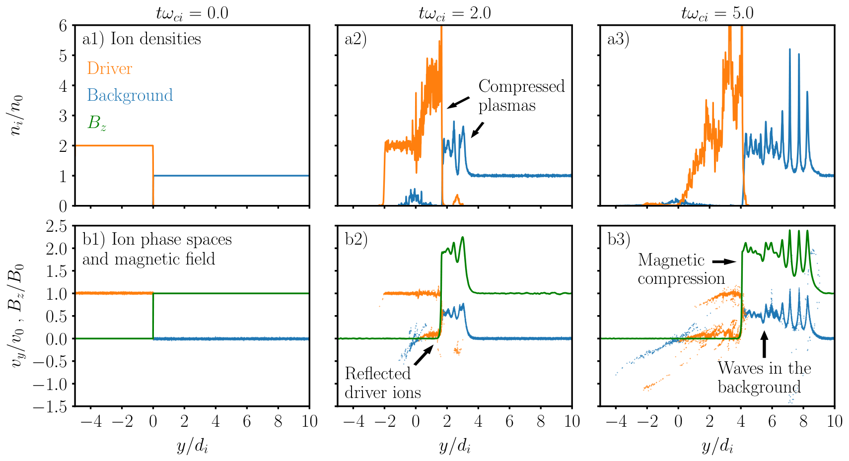
We see in Figs. 3 a1–3) that, as the driver flows to the right, it pushes the background plasma and the magnetic field with it, leading to a relocation of the interface between the two plasmas and creating two high-density regions on both sides of the interface. During this process, the driver ions are mostly confined in the upstream region relative to the plasma flow, while the background ions are mostly confined downstream, with the exception of small amounts of the driver and background ions that entered the opposite regions in the initial times of the simulation Takezaki et al. 2016; Takezaki et al. 2021.
The magnetic field rapidly increases in the transition from the unmagnetized driver to the magnetized background, as we can see in Figs. 3 b1–3). Due to the large mass discrepancies between the electrons and the ions, the transition occurs over a length scale larger than the local electron gyroradius but much smaller than the local ion gyroradius, and so, in the interface region between the two plasmas, the driver electrons are effectively magnetized while the driver ions are unmagnetized. The space-charge separation creates a negative electric field in the direction that reflects the driver ions back upstream with a new velocity , and causes an electron drift, which leads to a diamagnetic current. This current expels the magnetic field upstream, creating a magnetic cavity with no magnetic field, while the field is compressed downstream Ripin et al. 1993; VanZeeland and Gekelman 2004; Collette and Gekelman 2010. A more detailed study of the electric fields of the transition region is presented in Appendix A.
The energy and momentum lost by the driver plasma during this process are transferred to the background region. The initially stationary background ions are accelerated and the magnetic field is compressed. From this interaction, the bulk of the driver, the compressed background, and the interface between the plasmas travel to the right through the region initially occupied by the background plasma. Additionally, during this process, multiple waves and instabilities form in the background region, as we see in Fig. 3 b3). We also observe that the size of the perturbed background region increases over time.
In Fig. 3, the magnetic field and the plasma densities of the system are not constant, however, some average quantities of the system do not change significantly over time. Such examples include the average velocity of the accelerated background ions and the average of the compressed magnetic field. We could, therefore, consider that the system achieves a quasi-steady-state regime and that it can be represented by its average properties, as we show in Sec. IV.
III.3 Magnetic field diagnostics
To comprehend the dynamics of these systems, it is important to investigate the evolution of the magnetic field since it can be used to determine the motion of the particles and the electric fields. Additionally, magnetic field diagnostics are widely used for fast-driven plasmas in laboratory experiments VanZeeland and Gekelman 2004; Schaeffer et al. 2018; Schaeffer et al. 2022. From Ampère’s law, the component of the current density is , and so, we can use to investigate changes in the magnetic field.
To illustrate these two important quantities, we show in Fig. 4 the temporal evolution of a) the variation of the magnetic field , where is the initial magnetic field, and b) the current density . To understand how the system depends on the initial parameters, these diagnostics are shown for three driver densities: 1) , 2) , and 3) , with and .

In Fig. 4 we observe the same main structures for the three driver densities. Similarly to the experiment in Fig. 1 a), and as discussed in Sec. III.2, while the driver flows against the background, it expels the magnetic field, creating a magnetic cavity with no magnetic field, as observed in Figs. 4 a1–3). This magnetic cavity expands over time, and its maximum extent increases with the driver density. This is expected since the energy and the pressure exerted by the driver increase with its density, improving the coupling between the plasmas Hewett, Brecht, and Larson 2011. The velocity at which the magnetic cavity travels through the background is designated by coupling velocity . This velocity is always lower than and increases with the driver density, as shown in Fig. 4.
After all the driver ions with velocity are reflected, the driver may not have enough energy to push the background any further, leading to the reflection of the magnetic cavity. This happens for and (at and , respectively). For , the reflected driver ions continue pushing the magnetic cavity through the background region, although at a lower velocity. We consider the stopping distance the distance that the magnetic cavity travels before the driver ions with velocity are fully reflected, i.e., during the main interaction of the system.
In Figs. 4 a1–3), we also observe the magnetic compression in the downstream region, where the background is located. While the compressed magnetic field is not constant, its average does not change significantly over time during the main interaction of the plasmas. The average ratio of compressed to the initial magnetic field is designated by compression ratio . Additionally, the extent of the background plasma with compressed magnetic field increases over time. The velocity at which the magnetic compression travels through the unperturbed background plasma is designated by front velocity . Fig. 4 shows that also increases with the driver density. After the driver’s reflection, the compressed plasma continues to move through the unperturbed background.
Figs. 4 b1–3) show the current densities for the different driver densities. The sudden increase in magnetic field from the magnetic cavity to the magnetized background plasma is supported by the diamagnetic current Collette and Gekelman 2010. In the background region, we also observe multiple current structures associated with the fast and slow magnetosonic (MS) waves that form in the background plasma Everson 2016; Schaeffer et al. 2018.
IV Coupling parameters
As discussed in Sec. III.2, for uniform densities, and if the plasmas are long enough, the system reaches a quasi-steady-state regime, where some average quantities do not change significantly over time. Under these conditions and assuming the MHD formalism, we can describe the system by three different regions with different magnetic and kinetic properties, as shown in Fig. 5.
The first region in Fig. 5 refers to the magnetic cavity, where . The driver plasma is located in this upstream region, and the ion motion of the driver can be described by two ion populations with velocities and . The second region refers to the magnetic compression, where the average magnetic field is . In this region, the background ions accelerated by the interaction with the driver plasma have an average velocity of . Finally, the third region refers to the background region that remains unperturbed by the interaction of the two plasmas. Here, the magnetic field is and the background ions have no flow velocity. These three regions are visible in Fig. 4.
The regions are separated by two discontinuities where the plasma properties change abruptly. Discontinuities and move through the simulation box with velocity and , respectively. Some physical quantities must be conserved from the upstream to the downstream side of the discontinuities. With these conservation laws, we can derive analytical expressions for the coupling parameters , , and .
IV.1 Jump conditions at the discontinuities
To derive expressions for the coupling parameters, we consider the system description in Fig. 5. In the reference frame of the discontinuities, and for a quasi-steady-state regime, the time derivatives can be dropped in the MHD and Maxwell’s equations.
In the upstream and downstream sides of each discontinuity, some physical quantities must be conserved, which leads to the Rankine-Hugoniot (R-H) jump conditions. For magnetic fields perpendicular to the plasma flows, these conditions lead to Kivelson and Kivelson 1995; Balogh and Treumann 2013; Thompson 2013; Vink 2020
| (2) | ||||
| (3) | ||||
| (4) | ||||
| (5) |
In the previous equations, stands for the difference of values of a quantity in the upstream and downstream regions, while , , and stand for the density, mass, and velocity of the ions, respectively, for the electron pressure, for the internal energy per unit mass, and for the magnetic field. Eq. (2) corresponds to Ohm’s law, and Eqs. (3) to (5) to the mass, momentum, and energy conservation laws. We can apply these equations to both discontinuities A and B in Fig. 5.
IV.2 R-H equations at discontinuity A
From Eq. (2), the quantity must be conserved in the reference frame of discontinuity . This leads to
| (6) |
By also applying Eqs. (3) and (5) to the discontinuity, we obtain
| (7) |
| (8) |
where , , and are the density, pressure, and internal energy density of the driver population with velocity . If we assume similar thermal properties for the two driver populations, the enthalpy terms in Eq. (8) cancel out. Eqs. (7) and (8) then lead to and , as expected.
Finally, from Eq. (4), the momentum must also be conserved, which leads to
| (9) |
where the factor of 2 considers both populations of driver ions with and velocities, corresponds to the electron pressure in the compressed background region, and , , and
| (10) |
To determine the other equations for the coupling parameters, we now apply Eqs. (2) to (5) to discontinuity .
IV.3 R-H equations at discontinuity B
By applying Eqs. (2) and (3) to the reference frame of discontinuity , we obtain
| (11) | ||||
| (12) |
where refers to the density of the compressed background plasma. Eqs. (11) and (12) show that the background density and magnetic field increase by the same ratio Schaeffer et al. 2015; Everson 2016. Eq. (11) also shows a dependency between the three coupling parameters , , and .
Using Eq. (4), we have from the momentum conservation in that
| (13) |
where is the initial background electron pressure, , and . With Eq. (5) and using , where is the adiabatic index, we obtain
| (14) |
Finally, Eqs. (13) and (14) allow us to derive an expression for the compression ratio Cairns and Grabbe 1994; Kivelson and Kivelson 1995; Everson 2016; Vink 2020
| (15) |
Eq. (15) shows an expression for as a function of the velocity of the discontinuity. By solving Eqs. (9), (11), and (15) numerically, we can determine the coupling parameters , , and with only the initial conditions of the system.
IV.4 Solutions for low Mach numbers
With Eqs. (9) and (15), and by using Eq. (13) to replace in Eq. (11), we obtain a set of three equations that relate the coupling parameters , , and with each other and with the initial parameters of the system. By solving these equations numerically, we can calculate these parameters for given initial conditions. In some regimes, however, it is possible to also obtain analytical expressions for the coupling parameters.
From Eq. (15), it can be shown that for cold plasmas, such that , and low Mach numbers, we can consider (see Appendix B). Replacing Eq. (15) by this approximation, and using Eqs. (9) and (11), we have that , , and are given by
| (16) | ||||
| (17) | ||||
| (18) |
These expressions depend only on the initial parameters of the system. We stress that , , and can be directly measured from the magnetic diagnostics of the experiments and of the simulations, and therefore, they can be used to evaluate the coupling between the plasmas and to estimate uncertain initial conditions of the system.
The equations shown here are only valid for the main interaction of the system, i.e., before all the driver ions get reflected. After the main interaction, these reflected ions may still have enough energy to continue pushing the background forward, creating a second interaction between the driver and the background, but with different parameters.
IV.5 Solutions for high Mach numbers
We can also obtain analytical expressions for the coupling parameters for cold plasmas and high Mach numbers, such that and . Under this conditions, Eqs. (9), (11), and (15) lead to
| (19) | |||
| (20) | |||
| (21) |
Eq. (19) represents the maximum value for the compression ratio, well-known in strong shock theory Kivelson and Kivelson 1995; Balogh and Treumann 2013; Vink 2020.
V Comparison between the equations and the simulations
V.1 Dependency on the driver density
After deriving analytical expressions that describe the coupling between the driver and background plasmas, we now verify the validity of Eqs. (16) to (18). For the study of ion-scale magnetospheres, we are interested in the cases where and . For these conditions, we can apply the solutions for low Mach numbers, represented in Sec. IV.4.
Fig. 6 shows the measured values for the coupling parameter ratios , , and , for multiple simulations with different Alfvénic Mach numbers and driver-to-background density ratios , with . The measured coupling parameters are plotted alongside the values calculated with Eqs. (16) to (18).
Fig. 6 confirms that Eqs. (16) to (18) can be used to describe the coupling of the system, for the regimes considered. In Fig. 6 a) we observe that the magnetic compression ratio increases with the driver density and the Mach number, since for these conditions, the magnetic field offers less resistance to the driver, leading to tighter compressions. We can also see that for some of the simulations with low driver densities and low Mach numbers, the driver is not capable of compressing the background, leading to a magnetic decompression with .
In Fig. 6 b), the measured coupling velocities of the simulations are consistent with Eq. (17). Similarly to the magnetic compression ratio, increases with the driver density and the Mach number. For the simulations with , we observe negative coupling velocities, meaning that the driver is pushed back by the background and that it is the background that transfers its energy and momentum to the driver plasma.
Finally, in Fig. 6 c), we see that the front velocity increases with the driver density but decreases with the Mach number. For low Mach numbers, we observe small discrepancies between the simulations and Eq. (18). These differences are mostly associated with the difficulty in measuring in this regime, due to low magnetic compressions, i.e., , and the presence of waves in the background plasma (see Fig. 3).
V.2 Dependency on the driver ion mass
To continue the validation of Eqs. (16) to (18), we now compare them in Fig. 7 to simulations with different driver-to-background ion mass ratios and different Alfvénic Mach numbers . The simulations consider .
Similarly to Fig. 6, the results of simulations with different ion masses are consistent with Eqs. (16) to (18). Once again, Eq. (18) overestimates the front velocities measured in the simulations for low Mach numbers, mainly due to the difficulty in measuring in these simulations. After confirming that we can use Eqs. (16) to (18) to estimate the coupling parameters for low Mach numbers, we now need to validate the obtained solutions for high Mach numbers.
V.3 Solutions for high Mach numbers
To study the coupling for higher Mach numbers, we performed additional simulations with . To ensure that a quasi-steady-state was observed in these regimes and that we could measure with a sufficiently large compressed background region, we considered longer plasmas for these new simulations, namely for the driver and for the background.
Fig. 8 compares the different solutions obtained for the coupling parameters , , and , with the values measured in the simulations, for multiple Mach numbers , and the density ratios , , and . The simulations represented considered . Since the background magnetic field is aligned along , the heat flow should only be negligible in the and directions. As a result, the solutions presented in Fig. 8 consider for the perpendicularly magnetized background plasma Pudovkin et al. 1997; Pudovkin, Meister, and Besser 1999; Kim et al. 2021.
As we can observe in Fig. 8, the coupling parameters measured in the simulations are consistent with the solutions obtained by numerically solving Eqs. (9), (11), and (15). As expected, Eqs. (16) to (18) are also consistent with the numerical solutions for low Mach numbers, while Eqs. (19) to (21) are consistent for high Mach numbers. Unlike the analytical solution for for low Mach numbers, which corresponds to Eq. (16), the numerical solution predicts the saturation of the compression ratio for high Mach numbers. For and , we have .
In Fig. 8 c) we also observe that Eq. (18), the analytical solution for the front velocity and low Mach numbers , is similar to the numerical solution and the values measured in the simulations, in particular, for the lower density ratios. If we then calculate with Eq. (18), such that
| (22) |
and replace it in Eq. (15), we obtain an additional analytical solution for that works for all Mach number regimes. As we can see in Fig. 8 a) with the solid lines, this new analytical solution is a good approximation to the values measured in the simulations and in the numerical solutions.
After confirming that we can describe the coupling between the plasmas with the initial parameters of the system, both analytically and numerically, we can now use the obtained solutions to evaluate other characteristics of the system.
V.4 Stopping distance of the magnetic cavity
Figs. 6, 7, and 8 showed that we can use Eqs. (16) to (18) and Eqs. (19) to (21) to describe how the system evolves over time, for low and high Mach numbers, respectively. These equations are also useful to obtain other parameters, such as the stopping distance , i.e., the maximum distance that the magnetic cavity can travel through the background region, during the main interaction of the system.
The reflection time of the magnetic cavity also corresponds to the reflection time of the driver by the background plasma. The magnetic cavity travels a distance through the background region, with velocity , while the driver, with a length , travels with a velocity , relative to the driver-background boundary. The stopping distance can then be described by
| (23) |
Contrary to previously derived expressions for the stopping distance that only consider the driver energy transfer to the magnetic field, for sub-Alfvénic regimes Zakharov et al. 1999; Ripin et al. 1993; Clark et al. 2013; Clark et al. 2014; Behera, Kumar, and Singh 2021, or that only consider the driver energy transfer to the background kinetic energy, for super-Alfvénic regimes Winske and Gary 2007; Clark et al. 2013; Clark et al. 2014, Eq. (23) considers both the background kinetic and magnetic energy transfers and the energy of the reflected driver particles. By using Eq. (17) for low Mach numbers, the stopping distance becomes
| (24) |
Fig. 9 compares Eq. (24) with the measured stopping distance in the simulations. Fig. 9 a) shows the results for different driver-to-background density ratios and different Alfvénic Mach numbers , with , and Fig. 9 b) for different driver-to-background ions mass ratios and , with .
Fig. 9 shows good agreement between Eq. (24) and the stopping distances measured in the simulations. For high Mach numbers, densities, and mass ratios, Eq. (24) starts to overestimate the stopping distances. As we observed in Fig. 6 b) and Fig. 7 b), for these parameters, the coupling velocity is close to . Since the stopping distance is proportional to , small discrepancies between Eq. (17) and the simulations may lead to large differences in the values, for these conditions.
For high Mach numbers, and using Eq. (20), the stopping distance is given by
| (25) |
To also validate the solutions for high Mach numbers, Fig. 10 compares the values measured in the simulations with the obtained solutions for the different Mach number regimes. The simulations consider and the density ratios and .
Similarly to Fig. 8, Fig. 10 shows that the stopping distance calculated with Eq. (23) and the numerical solutions of are consistent with the values measured in the simulations, from low to high Mach numbers. Additionally, Eq. (24) is consistent with the simulations for low Mach numbers, while Eq. (25) is consistent with the simulations for high Mach numbers. In some of the high simulations, some “foot” structures were observed in the driver-background interface, leading to some uncertainty in the measured values of the stopping distance.
VI Applications to experiments and simulations
Eqs. (16) to (18) relate the different coupling parameters with the initial conditions of the system, for the low Mach numbers expected for the experiments with ion-scale magnetospheres. To validate the developed model, we now compare it with results from experiments with laser-driven plasmas and magnetized background plasmas. In particular, we compare the model with runs from LAPD experiments that observed strong coupling between the two plasmas.
The data chosen for these experiments are shown in Table 1. The typical laser-driven plasmas produced in the laboratory are not uniform in density and velocity as our coupling model considers. However, under small scales of the driver expansion and for the strong coupling regimes of the selected runs, some features remain similar to our 1D simulations, such as constant coupling and front velocities, and a plateau region on the magnetic field compression. In these conditions, we can partially apply the coupling study to experiments.
| Run | (km/s) | (km/s) | (km/s) | |||
|---|---|---|---|---|---|---|
| Run4 2013 Everson 2016 | 280 | 164 | 250 | 1.6 | 0.6 | 0.9 |
| Run3 2015 Schaeffer et al. 2015 | 189 | 260 | 440 | 2.0 | 1.4 | 2.3 |
| Mini Mag. Schaeffer et al. 2022 | 378 | 135 | 380 | 1.3 | 0.4 | 1.0 |
Since the experimental driver is not uniform and we do not have accurate measurements of the density, length, and velocity of the plasma, we cannot properly calculate the corresponding quantity in these experiments. With Eqs. (16) to (18), we obtain , and . We can use these relations to verify experimentally the validity of our model.
For the first and second runs in Table 1, we have an average compression of , leading to strong coupling between the plasmas. For the first run, we observe , as expected from the coupling model. However, we also observe . For the second run, we observe , but also . These differences from the coupling model may have emerged from the typical deceleration of the cavity and compression expansions observed in experiments Ripin et al. 1993; Schaeffer et al. 2015; Everson 2016; Winske et al. 2019, and from the difficulty in measuring precisely some of the coupling parameters from the available data.
In the last row of Table 1, we have the coupling parameters for the experiments with ion-scale magnetospheres Schaeffer et al. 2022, for the no dipole case, represented in Fig. 1 a). Since , this run has weaker coupling between the plasmas than the two previous cases Schaeffer et al. 2015; Everson 2016. We observe , but . In this run, the plasmas are short and do not interact with each other for enough time to observe a plateau region in the magnetic compression.
We can also apply the coupling study to estimate the spatial and temporal scales of laboratory ion-scale magnetospheres in experimental Schaeffer et al. 2022 and numerical Cruz et al. 2022 studies. As discussed in Sec. II, these systems consider a driver plasma and magnetized background plasma, with a dipolar magnetic field centered in the background. The pressure balance in Eq. (1) that describes the magnetopause current observed in Fig. 2 b) depends on the parameters of the system after the driver and background plasmas interact with each other and start moving towards the dipole. Since these parameters depend on , , and , which can be calculated with Eqs. (16) to (18) for the expected low Mach numbers in the laboratory Schaeffer et al. 2022, we can use the coupling study to obtain more accurately the pressure balances described by Eq. (1) that determine the standoff locations in ion-scale magnetospheres.
Furthermore, to observe the magnetopause under this setup, we must make sure that the driver has sufficient energy to push enough background plasma toward the dipole. With Eq. (23), we can determine how further can the driver plasma travel, and with Eq. (1), we can determine the effective size of the magnetosphere. Using these two quantities, we can estimate if the driver has enough energy to ensure the observation of a laboratory ion-scale magnetosphere, in the experiments and the simulations.
VII Discussion and conclusions
In recent experiments on the Large Plasma Device (LAPD) at UCLA, ion-scale magnetospheres were performed in the laboratory by driving a laser-produced plasma into a dipolar magnetic field embedded in a uniformly magnetized plasma. Under this configuration, the laser-driven and background plasmas first interact with each other before interacting with the strong magnetic field of the dipole. For the experimental and numerical analysis of laboratory ion-scale magnetospheres, and for the design of future experiments that involve fast plasmas moving toward magnetized plasmas, it is necessary to understand this interaction.
In this paper, we derived analytical expressions for magnetic field parameters that describe the coupling between an unmagnetized driver plasma and a perpendicularly magnetized background plasma. These expressions were then compared with 1D particle-in-cell (PIC) simulations for multiple densities, ion masses, and magnetic field values. For the cold plasmas, and uniform density and velocity profiles considered, the expressions were consistent with simulations. These expressions allow us to (i) evaluate the coupling between the plasmas, (ii) estimate initial quantities from simple magnetic field diagnostics, and (iii) calculate the spatial and temporal scales of these systems.
For the ideal plasmas considered, the simulations reached a near steady-state condition, where the coupling parameters — the average magnetic compression ratio and the velocities of the magnetic cavity and of the magnetic compression — remain constant. These quantities describe the coupling between the plasmas and increase with higher driver-to-background density and ion mass ratios. The compression ratio and the cavity velocity also increase with the Alfvénic Mach number, while the compression velocity decreases. Additionally, for some parameters, the driver plasma does not have enough momentum to push the background forward.
From conservation arguments, we obtained analytical expressions and numerical solutions for the coupling parameters, which were consistent with 1D PIC simulations. Since these parameters can be measured from magnetic field diagnostics, they can be used as a benchmark for the initial conditions of these systems. With these expressions, we can also determine other quantities, such as the stopping distance of the magnetic cavity and the magnetopause position associated with the laboratory ion-scale magnetospheres.
We assumed uniform profiles and long plasmas for the coupling model, and always observed strong coupling and a quasi-steady-state regime in the simulations. In the experiments with laser-driven plasmas and magnetized background plasmas, however, the driver is short, non-uniform, and expanding, and therefore, we do not always observe the same conditions. A complete study of the experimental coupling between the plasmas must consider these characteristics.
In conclusion, we derived analytical expressions for multiple parameters and arbitrary Alfvénic flows that describe the coupling between a driven plasma and a magnetized background plasma. These expressions are consistent with results from PIC simulations and can assist in the design of future experiments with driven plasmas and magnetized obstacles. For future works, we intend to explore other regimes and configurations, such as higher ion and electron temperatures, shorter drivers, and non-uniform densities and velocities.
Acknowledgements.
We acknowledge the support of the European Research Council (InPairs ERC-2015-AdG 695088), FCT (PD/BD/114307/2016, APPLAuSE PD/00505/2012, and UID/FIS/50010/2023), the NSF/DOE Partnership in Basic Plasma Science and Engineering (Award Number PHY-2010248), and PRACE for awarding access to MareNostrum (Barcelona Supercomputing Center, Spain). The simulations presented in this work were performed at the IST cluster (Lisbon, Portugal) and at MareNostrum.Data Availability Statement
The data that support the findings of this study are openly available in Zenodo at http://doi.org/10.5281/zenodo.7485077, reference number Cruz et al. 2023.
Appendix A Electric field of the system
For the collisionless, magnetic pressure dominated (, where and are the electron density and temperature, respectively), and low Mach numbers () considered, neither collisions nor instabilities effectively transfer momentum and energy between the driver and the perpendicularly magnetized background plasma. For these conditions, the laminar electric field provides the dominant coupling mechanism between the two plasmas Everson 2016. Using a hybrid model Bondarenko et al. 2017, where the ion species are considered kinetically, and the electron species as a charge-neutralizing fluid, and considering that the magnetic field is mostly defined in the direction, then the laminar collisionless electric field of the system, for the regimes considered, is approximately given by
| (26) |
In Eq. (26), is the current density of the driver () or of the background () plasmas. , , and are the ions’ charge, density, and velocity, respectively, for the plasma . With quasi-neutrality, we have . The first term in Eq. (26), , is primarily defined along the direction since . The second term, , however, is mostly defined in , with , since the ion motions are mostly defined along . The third term is associated with the electron pressure .
To verify if Eq. (26) correctly describes the electric field of the system, the terms in Eq. (26) and the electric field of the simulation with , , and (previously presented in Fig. 3), are compared in Fig. 11, for .
Fig. 11 shows that we can use Eq. (26) to calculate the electric field of these systems. In Fig. 11 a), we see that the component of the electric field can be expressed by , which depends on the magnetic field gradient. Within the interface that separates the magnetic cavity from the compressed magnetic field, we observe a significant negative electric field. This electric field is responsible for the reflection of the driver ions back to the upstream region.
Fig. 11 b) also shows that the component of the electric field can be described by . In the background region, is always negative and approximately , in agreement with Ohm’s law, . For the low Mach numbers and low considered, is typically negligible when compared to the electric field terms and .
We can use Eq. (26) to describe the motion of the particles, in particular, the reflection of the driver particles by the background plasma region. Near this region, unmagnetized driver ions move with velocity against the compressed background magnetic field of average value . The discontinuity region (labeled as in Fig. 5) moves with velocity , and the driver ions end up reflected upstream with velocity . From Eq. (26), this field is approximately given by
| (27) |
Since for this region, the equation of motion for a reflecting driver ion is
| (28) |
where is the driver ion velocity in the reference frame of the discontinuity. In this frame, the driver ions have initial velocity and start to be reflected upstream when . By integrating Eq. (28), and considering as the average electron pressure of the compressed background plasma, we obtain
| (29) |
We consistently observed a peak in the electron density of in the interface driver-background of the simulations. Assuming this value in Eq. (29), we end up with
| (30) |
which corresponds to the pressure balance of Eq. (9) for , as expected.
Appendix B Energy expressions
To validate the assumption for low Mach numbers considered in Sec. IV.3, we now compare the different energy fluxes terms represented in Eq. (5) with the total energies measured in multiple simulations. Considering , , , and the energy fluxes of the system associated with the driver plasma, background plasma, magnetic field, and electric field, respectively, in the lab frame, over a time and transverse area , we must have, due to energy conservation
| (31) |
In Fig. 5, we observe that the driver consists of two populations, with velocity and . The energy flux of each population can be calculated by multiplying the kinetic energy of each ion with the rate of the number of ions. Recalling from Sec. IV.2 that and , the interface driver-background travels with velocity , and assuming cold plasmas (), we obtain that the driver energy flux in the lab frame can be calculated with
| (32) |
Unlike the driver, the background plasma is located in two different regions in Fig. 5. In the magnetic compression region, the average kinetic energy flow of each background ion is , and the density is . In the unperturbed background region, the background plasma has no flow velocity. For low Mach numbers and cold plasmas, we can ignore the contribution of the compressed background electron pressure . Since the back and front boundaries of the compression region travel with velocities and , respectively, we can then express the background energy flux associated with the plasmas flow as
| (33) |
Finally, we need an expression for the magnetic energy flux. The magnetic compression region has an average magnetic field of and increases its length at a velocity , while the unperturbed background region has a magnetic field and a length that decreases at a velocity . The magnetic energy flux is thus
| (34) |
To validate the previous expressions for the energy fluxes, we performed multiple simulations with different Alfvénic Mach numbers and driver-to-background density ratios , with . For each simulation, we measured the coupling parameters and from the magnetic field data, and then, with these values, we calculated the theoretical energy fluxes with Eqs. (32) to (34).
In Fig. 12, the calculated energy fluxes of a) the driver plasma and b) the magnetic field are compared to the correspondent energy fluxes obtained from the variation of the total energies in the simulations. Each quantity was measured in the quasi-steady-state regime of the simulations.
Fig. 12 confirms that Eqs. (32) and (34) can be used to describe the driver and magnetic energy fluxes of the system, for the regimes considered. In Fig. 12 a) we observe that the flux of energy lost by the driver increases for higher driver densities and lower Mach numbers, leading to a more efficient energy transfer from the driver to the background. Similarly, in Fig. 12 b), the magnetic energy flux is larger for denser drivers and lower Mach numbers.
In Fig. 12, we also observe that in the simulation with and , it is the magnetic field that transfers energy to the driver plasma. This simulation corresponds approximately to the case where the initial magnetic pressure is larger than the driver’s ram pressure (i.e., ), and so, the driver is pushed back by the background, leading to a negative coupling velocity.
Fig. 13 a) compares the background energy flux calculated with Eq. (33) with the energy flux obtained from the total energy of the simulations. As we can see, Eq. (33) is more consistent with the simulations for low Mach numbers, than for high Mach numbers and driver densities.
For high Mach numbers, instabilities start to form in the background plasma. This leads to an increase in the thermal energy of the plasma, which starts to have an important role in the energy partition of the system. Since Eq. (33) neglects instabilities and thermal effects, it underestimates the energy flux of the background plasma, as we observe in Fig. 13 a). Fig. 13 b) shows the average ratio of thermal energy of the background ions to their total energy , near the final stage of the main interaction in the simulations. As expected, we observe that, for high Mach numbers and driver densities, a significant percentage of the background ions’ energy is thermal energy, while for low Mach numbers, the thermal energy is negligible.
The thermal effects of the ions in the compressed background can be estimated with the pressure . If we assume Eqs. (16) and (18) for and , respectively, and apply Eq. (13), we obtain that the ratio of the plasma pressure to magnetic pressure in the compressed background region is given by
| (35) |
As we can see in Fig. 6, the coupling velocity increases with the Mach number and the density ratio , while the front velocity decreases with but increases with . As a result, the ratio in Eq. (35) decreases for low Mach numbers. In this regime, we can then ignore the term in the energy conservation.
By applying Eqs. (32) to (34) in Eq. (31), it is possible to show that for low Mach numbers. Additionally, we obtain from Eq. (15) for and that for , , and . As a result, we observe that Eq. (15) follows for low Mach numbers .
From Eqs. (32) and (33), we also obtain that the ratio of energy transferred from the driver plasma to the background plasma is
| (36) |
The ratio between the velocities of the magnetic cavity and of the magnetic compression is then a direct tool to evaluate the efficiency of the energy transfer from the driver to the background plasmas.
References
- Burlaga et al. (2001) L. F. Burlaga, R. M. Skoug, C. W. Smith, D. F. Webb, T. H. Zurbuchen, and A. Reinard, “Fast ejecta during the ascending phase of solar cycle 23: ACE observations, 1998-1999,” Journal of Geophysical Research: Space Physics 106, 20957–20977 (2001).
- Spicer et al. (1990) D. S. Spicer, R. W. Clark, S. P. Maran, and R. W. Clark, “A Model of the Pre-Sedov Expansion Phase of Supernova Remnant-Ambient Plasma Coupling and X-Ray Emission from SN 1987A,” Astrophysical Journal; (USA) 356, 549 (1990).
- Mendis and Ip (1977) D. Mendis and W.-H. Ip, “The ionospheres and plasma tails of comets,” Space Science Reviews 20, 145–190 (1977).
- Krimigis et al. (1982) S. M. Krimigis, G. Haerendel, R. W. McEntire, G. Paschmann, and D. A. Bryant, “The active magnetospheric particle tracer explorers (AMPTE) program,” Eos, Transactions American Geophysical Union 63, 843–850 (1982).
- Johnson and Kierein (1992) M. H. Johnson and J. Kierein, “Combined release and radiation effects satellite (crres): Spacecraft and mission,” Journal of Spacecraft and Rockets 29, 556–563 (1992).
- Dyal (2006) P. Dyal, “Particle and field measurements of the starfish diamagnetic cavity,” Journal of Geophysical Research: Space Physics 111 (2006), https://doi.org/10.1029/2006JA011827.
- Hewett, Brecht, and Larson (2011) D. W. Hewett, S. H. Brecht, and D. J. Larson, “The physics of ion decoupling in magnetized plasma expansions,” Journal of Geophysical Research: Space Physics 116 (2011), https://doi.org/10.1029/2011JA016904.
- Winske and Gary (2007) D. Winske and S. P. Gary, “Hybrid simulations of debris-ambient ion interactions in astrophysical explosions,” Journal of Geophysical Research: Space Physics 112 (2007), https://doi.org/10.1029/2007JA012276.
- Gurnett et al. (1986) D. A. Gurnett, R. R. Anderson, T. Z. Ma, G. Haerendel, G. Paschmann, O. H. Bauer, R. A. Treumann, H. C. Koons, R. H. Holzworth, and H. Lühr, “Waves and electric fields associated with the first ampte artificial comet,” Journal of Geophysical Research: Space Physics 91, 10013–10028 (1986).
- Ip and Axford (1987) W. H. Ip and W. I. Axford, “The formation of a magnetic-field-free cavity at comet Halley,” (1987).
- Bernhardt (1992) P. A. Bernhardt, “Probing the magnetosphere using chemical releases from the combined release and radiation effects satellite,” Physics of Fluids B: Plasma Physics 4, 2249–2256 (1992).
- Zakharov et al. (1999) Y. Zakharov, M. Alexandr, P. Amold, and P. Vitali, “Diamagnetic cavity of plasma clouds expanding in magnetized media,” Journal of Plasma and Fusion Research 2, 398 (1999).
- Collette and Gekelman (2010) A. Collette and W. Gekelman, “Structure of an exploding laser-produced plasma,” Phys. Rev. Lett. 105, 195003 (2010).
- Goetz, C. et al. (2016) Goetz, C., Koenders, C., Richter, I., Altwegg, K., Burch, J., Carr, C., Cupido, E., Eriksson, A., Güttler, C., Henri, P., Mokashi, P., Nemeth, Z., Nilsson, H., Rubin, M., Sierks, H., Tsurutani, B., Vallat, C., Volwerk, M., and Glassmeier, K.-H., “First detection of a diamagnetic cavity at comet 67p/churyumov-gerasimenko,” A&A 588, A24 (2016).
- Schaeffer et al. (2018) D. B. Schaeffer, L. R. Hofer, E. N. Knall, P. V. Heuer, C. G. Constantin, and C. Niemann, “A platform for high-repetition-rate laser experiments on the large plasma device,” High Power Laser Science and Engineering 6, e17 (2018).
- Winske et al. (2019) D. Winske, J. D. Huba, C. Niemann, and A. Le, “Recalling and updating research on diamagnetic cavities: Experiments, theory, simulations,” Frontiers in Astronomy and Space Sciences 5 (2019), 10.3389/fspas.2018.00051.
- Ripin et al. (1993) B. H. Ripin, J. D. Huba, E. A. McLean, C. K. Manka, T. Peyser, H. R. Burris, and J. Grun, “Sub-alfvénic plasma expansion,” Physics of Fluids B: Plasma Physics 5, 3491–3506 (1993).
- VanZeeland and Gekelman (2004) M. VanZeeland and W. Gekelman, “Laser-plasma diamagnetism in the presence of an ambient magnetized plasma,” Physics of Plasmas 11, 320–323 (2004).
- Bonde (2018) J. Bonde, “Collisionless coupling of a high- expansion to an ambient, magnetized plasma. i. rayleigh model and scaling,” Physics of Plasmas 25, 042109 (2018).
- Bonde, Vincena, and Gekelman (2018) J. Bonde, S. Vincena, and W. Gekelman, “Collisionless coupling of a high- expansion to an ambient, magnetized plasma. ii. experimental fields and measured momentum coupling,” Physics of Plasmas 25, 042110 (2018).
- Le et al. (2021) A. Le, D. Winske, A. Stanier, W. Daughton, M. Cowee, B. Wetherton, and F. Guo, “Astrophysical explosions revisited: Collisionless coupling of debris to magnetized plasma,” Journal of Geophysical Research: Space Physics 126, e2021JA029125 (2021).
- Behera, Kumar, and Singh (2021) N. Behera, A. Kumar, and R. K. Singh, “Cavitation and charge separation in laser-produced copper and carbon plasma in transverse magnetic field,” Plasma Research Express 3, 025011 (2021).
- Clark et al. (2014) S. E. Clark, E. T. Everson, D. B. Schaeffer, A. S. Bondarenko, C. G. Constantin, C. Niemann, and D. Winske, “Enhanced collisionless shock formation in a magnetized plasma containing a density gradient,” Phys. Rev. E 90, 041101 (2014).
- Bondarenko et al. (2017) A. S. Bondarenko, D. B. Schaeffer, E. T. Everson, S. E. Clark, B. R. Lee, C. G. Constantin, S. Vincena, B. Van Compernolle, S. K. Tripathi, D. Winske, and C. Niemann, “Collisionless momentum transfer in space and astrophysical explosions,” Nature Physics 13, 573–576 (2017).
- Clark, Denavit, and Papadopoulos (1973) R. W. Clark, J. Denavit, and K. Papadopoulos, “Laminar interactions in high Mach number plasma flows,” The Physics of Fluids 16, 1097–1101 (1973).
- Cairns and Grabbe (1994) I. H. Cairns and C. L. Grabbe, “Towards an mhd theory for the standoff distance of earth’s bow shock,” Geophysical Research Letters 21, 2781–2784 (1994).
- Clark et al. (2013) S. E. Clark, D. Winske, D. B. Schaeffer, E. T. Everson, A. S. Bondarenko, C. G. Constantin, and C. Niemann, “Hybrid simulation of shock formation for super-alfvénic expansion of laser ablated debris through an ambient, magnetized plasma,” Physics of Plasmas 20, 082129 (2013).
- Everson (2016) E. T. Everson, Magnetic Field Characterization of a Diamagnetic Cavity Piston for Generation of Quasi-Perpendicular Collisionless Shocks, Ph.D. thesis, University of California, Los Angeles (2016).
- Drake (2000) R. P. Drake, “The design of laboratory experiments to produce collisionless shocks of cosmic relevance,” Physics of Plasmas 7, 4690–4698 (2000).
- Niemann et al. (2014) C. Niemann, W. Gekelman, C. G. Constantin, E. T. Everson, D. B. Schaeffer, A. S. Bondarenko, S. E. Clark, D. Winske, S. Vincena, B. Van Compernolle, and P. Pribyl, “Observation of collisionless shocks in a large current-free laboratory plasma,” Geophysical Research Letters 41, 7413–7418 (2014).
- Niemann et al. (2013) C. Niemann, W. Gekelman, C. G. Constantin, E. T. Everson, D. B. Schaeffer, S. E. Clark, D. Winske, A. B. Zylstra, P. Pribyl, S. K. P. Tripathi, D. Larson, S. H. Glenzer, and A. S. Bondarenko, “Dynamics of exploding plasmas in a large magnetized plasma,” Physics of Plasmas 20, 012108 (2013).
- Schaeffer et al. (2015) D. B. Schaeffer, E. T. Everson, A. S. Bondarenko, S. E. Clark, C. G. Constantin, D. Winske, W. Gekelman, and C. Niemann, “Experimental study of subcritical laboratory magnetized collisionless shocks using a laser-driven magnetic piston,” Physics of Plasmas 22, 113101 (2015).
- Schaeffer et al. (2022) D. B. Schaeffer, F. D. Cruz, R. S. Dorst, F. Cruz, P. V. Heuer, C. G. Constantin, P. Pribyl, C. Niemann, L. O. Silva, and A. Bhattacharjee, “Laser-driven, ion-scale magnetospheres in laboratory plasmas. i. experimental platform and first results,” Physics of Plasmas 29, 042901 (2022).
- Gekelman et al. (1991) W. Gekelman, H. Pfister, Z. Lucky, J. Bamber, D. Leneman, and J. Maggs, “Design, construction, and properties of the large plasma research device-the lapd at ucla,” Review of Scientific Instruments 62, 2875–2883 (1991).
- Cruz et al. (2022) F. D. Cruz, D. B. Schaeffer, F. Cruz, and L. O. Silva, “Laser-driven, ion-scale magnetospheres in laboratory plasmas. ii. particle-in-cell simulations,” Physics of Plasmas 29, 032902 (2022).
- Fonseca et al. (2002) R. A. Fonseca, L. O. Silva, F. S. Tsung, V. K. Decyk, W. Lu, C. Ren, W. B. Mori, S. Deng, S. Lee, T. Katsouleas, and J. C. Adam, “OSIRIS: A three-dimensional, fully relativistic particle in cell code for modeling plasma based accelerators,” in Lecture Notes in Computer Science (including subseries Lecture Notes in Artificial Intelligence and Lecture Notes in Bioinformatics), Vol. 2331 LNCS (Springer Verlag, 2002) pp. 342–351.
- Fonseca et al. (2013) R. A. Fonseca, J. Vieira, F. Fiuza, A. Davidson, F. S. Tsung, W. B. Mori, and L. O. Silva, “Exploiting multi-scale parallelism for large scale numerical modelling of laser wakefield accelerators,” Plasma Physics and Controlled Fusion 55 (2013), 10.1088/0741-3335/55/12/124011.
- Zakharov (2003) Y. Zakharov, “Collisionless laboratory astrophysics with lasers,” IEEE Transactions on Plasma Science 31, 1243–1251 (2003).
- Cruz et al. (2023) F. D. Cruz, D. B. Schaeffer, F. Cruz, and L. O. Silva, “Strong collisionless coupling between an unmagnetized driver plasma and a magnetized background plasma,” (2023), https://doi.org/10.5281/zenodo.7485077.
- Takezaki et al. (2016) T. Takezaki, K. Takahashi, T. Sasaki, T. Kikuchi, and N. Harada, “Accelerated ions from pulsed-power-driven fast plasma flow in perpendicular magnetic field,” Physics of Plasmas 23, 062904 (2016).
- Takezaki et al. (2021) T. Takezaki, S. Kato, T. Oguchi, S. Watanabe, K. Takahashi, T. Sasaki, T. Kikuchi, and H. Ito, “Effect of multi-ion species on collisionless plasma driven by a compact plasma focus device in perpendicular magnetic field,” Physics of Plasmas 28, 102109 (2021).
- Kivelson and Kivelson (1995) M. G. Kivelson and M. G. Kivelson, Introduction to space physics (Cambridge university press, 1995).
- Balogh and Treumann (2013) A. Balogh and R. A. Treumann, Physics of collisionless shocks: space plasma shock waves (Springer Science & Business Media, 2013).
- Thompson (2013) W. B. Thompson, An introduction to plasma physics (Elsevier, 2013).
- Vink (2020) J. Vink, Physics and Evolution of Supernova Remnants (Springer, 2020).
- Pudovkin et al. (1997) M. I. Pudovkin, C.-V. Meister, B. P. Besser, and H. K. Biernat, “The effective polytropic index in a magnetized plasma,” Journal of Geophysical Research: Space Physics 102, 27145–27149 (1997).
- Pudovkin, Meister, and Besser (1999) M. Pudovkin, C.-V. Meister, and B. Besser, “Adiabatic indices in a convecting anisotropic plasma,” Astronomische Nachrichten 320, 87–93 (1999).
- Kim et al. (2021) J. Y. Kim, G. Go, Y. S. Hwang, and K.-J. Chung, “Dependence of the polytropic index of plasma on magnetic field,” New Journal of Physics 23, 052001 (2021).
*