跳到论文正文
W Papers独立论文阅读器 arXiv:2302.00061 论文正文 计算阅读时间 · 0%
引用这篇论文根据当前论文元数据生成,正式投稿前建议核对。


License: CC BY 4.0
arXiv:2302.00061v1 [cs.LG] 31 Jan 2023

Dynamic Flows on Curved Space Generated by Labeled Data

Xinru Hua Affiliation: Stanford University    Truyen Nguyen Affiliation: The University of Akron    Tam Le Affiliation: The Institute of Statistical Mathematics / RIKEN AIP    Jose Blanchet Affiliation: Stanford University    Viet Anh Nguyen Affiliation: Affiliation: Chinese University of Hong Kong
Abstract

The scarcity of labeled data is a long-standing challenge for many machine learning tasks. We propose our gradient flow method to leverage the existing dataset (i.e., source) to generate new samples that are close to the dataset of interest (i.e., target). We lift both datasets to the space of probability distributions on the feature-Gaussian manifold, and then develop a gradient flow method that minimizes the maximum mean discrepancy loss. To perform the gradient flow of distributions on the curved feature-Gaussian space, we unravel the Riemannian structure of the space and compute explicitly the Riemannian gradient of the loss function induced by the optimal transport metric. For practical applications, we also propose a discretized flow, and provide conditional results guaranteeing the global convergence of the flow to the optimum. We illustrate the results of our proposed gradient flow method on several real-world datasets and show our method can improve the accuracy of classification models in transfer learning settings.

1 Introduction

A major challenge in many data science applications is the scarcity of labeled data. Data augmentation methods have been studied in the literature; see for example, the noise injection methods Moreno-Barea et al. 2018, generative models Yi et al. 2019, and Shorten and Khoshgoftaar 2019 for a survey. We consider a setting where one domain has only a few labeled samples for each class, so we cannot train a well-performing classifier with the available data. To alleviate the data scarcity problem in this setting, we propose to enrich the target dataset by generating additional labeled samples. Using generative models is not possible in our setting because they usually require more than a few samples for each class to learn and generate high-quality new samples Gao et al. 2018. In our work, we choose a source dataset with extensive labeled data and then flow the labeled data to the target dataset. Precisely, we introduce a novel data augmentation methodology based on a gradient flow approach that minimizes the maximum mean discrepancy (MMD\mathrm{MMD}) distance between the target and the augmented data. Therefore, when minimizing the MMD\mathrm{MMD} distance, we are able to obtain an efficient scheme which generates additional labeled data from the target distribution. Our scheme is model-independent and can be applied to any datasets regardless of the number of classes or dimensionality.

Mathematically, we consider a feature space 𝒳=ℝm\mathcal{X}={\mathbb{R}}^{m} and a categorical label space 𝒴\mathcal{Y}. We have a source domain dataset consisting of NN samples (xi,yi)∈𝒳×𝒴(x_{i},y_{i})\in\mathcal{X}\times\mathcal{Y} for i=1,…,Ni=1,\ldots,N, and a target domain dataset of MM samples (x¯j,y¯j)∈𝒳×𝒴(\bar{x}_{j},\bar{y}_{j})\in\mathcal{X}\times\mathcal{Y} for j=1,…,M⁡(M≪N)j=1,\ldots,M(M\ll N). The ultimate goal of this paper is to generate new samples in the target domain, and we aim to generate new samples whose distribution is as close as possible to the distribution that governs the target domain.

We here introduce a gradient flow method Arbel et al. 2019; Mroueh et al. 2019 to synthesize new, unseen data samples. Gradient flow is a continuous flow along the path where a considered loss function decreases its value. Because we have extensive source domain samples, it is possible to flow each source sample towards the target data while minimizing the loss function. The terminal product of the flow will be new samples that can sufficiently approximate the distribution of the target domain. Thus, gradient flow is an approach to synthesize new target domain samples, and is a complement to data augmentation methods, like adding random noise.

Unfortunately, formulating a gradient flow algorithm for labeled data with categorical set 𝒴\mathcal{Y} is problematic. Indeed, there is no clear metric structure on 𝒴\mathcal{Y} in order to define the topological neighborhood, this in turn leads to the difficulty of forming the gradients with respect to the categorical component. To overcome this difficulty, we lift each individual label to a richer structure. For example, a label such as “0” is replaced by a mean vector and a covariance matrix based on the whole distribution of the information associated to this particular label. Then it will be much more natural to apply gradient flow algorithms in the space of the lifted representation. A gradient flow on the dataset space with this idea was recently proposed in Alvarez-Melis and Fusi 2021 by leveraging a new notion of distance between datasets in Alvarez-Melis and Fusi 2020; Courty et al. 2017; Damodaran et al. 2018. The main idea behind this approach is to reparametrize the categorical space 𝒴\mathcal{Y} using the conditional distribution of the features, which is assumed to be Gaussian, and then construct a gradient flow on the feature-Gaussian space. Nevertheless, the theoretical analysis in Alvarez-Melis and Fusi 2021 focuses solely on the gradients with respect to the feature with no treatment of the flow with respect to the Gaussian component. In fact, the space of Gaussian distributions is not a (flat) vector space, and extracting gradient information depends on the choice of the metric imposed on this Gaussian space. On the other hand, our method computes the full gradient with respect to the Gaussian component (the mean and covariance matrix component that correspond to the label component).

Paper Dataset
On curved Riemannian space
Gradient has mean
and covariance component
Alvarez-Melis and Fusi 2021 synthetic, *NIST, and CIFAR10
Arbel et al. 2019 synthetic
Ours synthetic, *NIST, and TinyImageNet ✓ ✓
Table 1: To the best of our knowledge, we provide the first results on the full gradient of the features and lifted labels on a curved Riemannian space. We also conduct numerical experiments on the highest-dimension real-world datasets.

Our gradient flows minimize the MMD\mathrm{MMD} loss function, thus it belongs to the family of MMD\mathrm{MMD} gradient flows that was pioneered in Mroueh et al. 2019; Arbel et al. 2019, and further extended in Mroueh and Nguyen 2021. The MMD\mathrm{MMD} function compares two distributions via their kernel mean embeddings on a flat reproducing kernel Hilbert space (RKHS). In contrast to the Kullback-Leibler divergence flow, the MMD\mathrm{MMD} flow can employ a sample approximation for the target distribution Liu 2017. Further, the squared MMD\mathrm{MMD} possesses unbiased sample gradients Bińkowski et al. 2018; Bellemare et al. 2017. However, existing literature on MMD\mathrm{MMD} flows focus on distributions on flat Euclidean spaces. The flow developed in our paper here is for distributions on a curved Riemannian feature-Gaussian space. Moreover, our approach is distinctive from the flow in Alvarez-Melis and Fusi 2021 because we impose a specific metric on the Gaussian component, and we compute explicitly the Riemannian gradient of the MMD\mathrm{MMD} loss function with respect to this metric to formulate our flow. Table 1 compares our work with two recent papers on gradient flow in theory and numerical experiments.

Recently, generative models Rezende et al. 2016; Wang et al. 2021 are successful in generating image samples from given distributions. The most important difference with our method is that generative models learn a prior distribution from massive data that are similar to the target data and generate new target samples conditioning on the prior distribution Wang et al. 2020; Gao et al. 2018. Comparatively, our algorithm can transfer between two non-similar and non-related distributions, for example, from random Gaussian noise to MNIST in Supplementary B.11. Another benefit of our method is that we provide conditions for global convergence of our algorithms in Section 4, whereas generative models or more specific, generative adversarial networks (GANs), currently do not guarantee global convergence Wiatrak et al. 2019.

The application of our gradient flow is few-shot transfer learning, where we want to train classifiers with limited labeled data in the target domain. The numerical experiments in Section 5 demonstrate that our gradient flows can effectively augment the target data, and thus can significantly boost the accuracy in the classification task in the few-shot learning setting. Moreover, we run experiments on Tiny ImageNet datasets to highlight that our algorithm is scalable to higher-dimensional image data, that is higher than recent gradient flow works Alvarez-Melis and Fusi 2021; Fan and Alvarez-Melis 2022. We also compare our method with Alvarez-Melis and Fusi 2021, mixup method Zhang et al. 2017, and traditional data augmentation methods. Results in Supplementary B.8–B.10 show that our method improves the accuracy in transfer learning more than these methods.

Some related works study nonparametric gradient flows using the 22-Wasserstein distance between distributions Ambrosio et al. 2008; Jordan et al. 1998; Otto 2001; Villani 2008; Santambrogio 2015; Santambrogio 2017; Frogner and Poggio 2020, but only for distributions on Euclidean spaces and a different distance. Nonparametric gradient flows with other metrics include Sliced-Wasserstein Descent Liutkus et al. 2019, Stein Descent Liu 2017; Liu and Wang 2016, and Sobolev Descent Mroueh et al. 2019. However, they also only consider distributions on Euclidean spaces. In particular, Liu 2017 introduce Riemannian structures for the Stein geometry on flat spaces, while ours is for an optimal transport metric on a curved space. Parametric flows for training GANs are studied in Chizat and Bach 2018; Chen and Li 2018; Arbel et al. 2020; Mroueh and Nguyen 2021.

Contributions.

We study a gradient flow approach to synthesize new labeled samples related to the target domain. To construct this flow, we consider the space of probability distributions on the feature-Gaussian manifold, and we are metrizing this space with an optimal transport distance. We summarize the contributions of this paper as follows.

  • •

    We study in details the Riemannian structure of the feature-Gaussian manifold in Section 3, as well as the Riemannian structure of the space of probability measures supported on this manifold in Supplementary A.1.

  • •

    We consider a gradient flow that minimizes the squared MMD\mathrm{MMD} loss function to the target distribution. We describe explicitly the (Riemannian) gradient of the squared MMD\mathrm{MMD} in Lemma 5, and we provide a partial differential equation describing the evolution of the gradient flow that follows the (Riemannian) steepest descent direction.

  • •

    We propose two discretized schemes to approximate the continuous gradient flow equation in Section 4.1 and 4.2. We provide conditions guaranteeing the global convergence of our gradient flows to the optimum in both schemes.

  • •

    In Section 5, we demonstrate numerical results with our method on real-world image datasets. We show that our method can generate high-fidelity images and improve the classification accuracy in transfer learning settings.

Notations.

We use 𝕊n{\mathbb{S}}^{n} to denote the set of n×nn\times n real and symmetric matrices, and 𝕊+⁣+n⊂𝕊n{\mathbb{S}}^{n}_{++}\subset{\mathbb{S}}^{n} consists of all positive definite matrices. For A∈𝕊nA\in{\mathbb{S}}^{n}, tr​(A)≔∑iAi​i\text{tr}(A)\coloneqq\sum_{i}A_{ii}. We use ⟨⋅,⋅⟩\langle\cdot,\cdot\rangle and ∥⋅∥2\|\cdot\|_{2} to denote the standard inner product and norm on Euclidean spaces. Let 𝒫⁡(X){\mathcal{P}}(X) be the collection of all probability distributions with finite second moment on metric space XX. If φ:X→Y\varphi:X\to Y is a Borel map and ν∈𝒫⁡(X)\nu\in{\mathcal{P}}(X), then the push-forward φ#​ν\varphi_{\#}\nu is the distribution on YY given by φ#​ν​(E)=ν⁡(φ−1​(E))\varphi_{\#}\nu(E)=\nu(\varphi^{-1}(E)) for all Borel sets E⊂YE\subset Y. For a function ff of the continuous time variable tt, ftf_{t} denotes the value of ff at tt while ∂tf\partial_{t}f denotes the standard derivative of ff w.r.t. tt. Also, δz\delta_{z} denotes the Dirac delta measure at zz.

All proofs are provided in the Supplementary material.

2 Labeled Data Synthesis via Gradient Flows of Lifted Distributions

In this section, we describe our approach to synthesize target domain samples using gradient flows. A holistic view of our method is presented in Fig. 1.

Refer to caption
Figure 1: Schematic view of our approach: The source and target datasets are first lifted to distributions ρ0\rho^{0} and ϱ\varrho on the feature-Gaussian space (left box). We then run a gradient flow for TT iterations to get a terminal distribution ρT\rho^{T} (middle). Atoms of ρT\rho^{T} are projected to get labeled target samples (right).

In the first step, we would need to lift the feature-label space 𝒳×𝒴\mathcal{X}\times\mathcal{Y} to a higher dimensional space where a metric can be defined. Consider momentarily the source data samples (xi,yi)i=1N(x_{i},y_{i})_{i=1}^{N}. Notice that this data can be represented as an empirical distribution ν\nu on 𝒳×𝒴\mathcal{X}\times\mathcal{Y}. More precisely, we have ν=N−1​∑i=1Nδ(xi,yi)\nu=N^{-1}\sum_{i=1}^{N}\delta_{(x_{i},y_{i})}. As 𝒴\mathcal{Y} is discrete, the law of conditional probabilities allows us to dis-integrate ν\nu into the conditional distributions νy\nu_{y} of X|Y=yX|Y=y satisfying ν⁡(E×F)=∫Fνy​(E)​ν2​(𝑑y)\nu(E\times F)=\int_{F}\nu_{y}(E)\nu^{2}(\mathrm{d}y) for every E⊂𝒳E\subset\mathcal{X} and F⊂𝒴F\subset\mathcal{Y}, where ν2≔N−1​∑i=1Nδyi\nu^{2}\coloneqq N^{-1}\sum_{i=1}^{N}\delta_{y_{i}} is the second marginal of ν\nu (Ambrosio et al. 2008, Theorem 5.3.1). The lifting procedure is obtained by employing a pre-determined mapping ϕ:𝒳→ℝn\phi:\mathcal{X}\to{\mathbb{R}}^{n}, and any categorical value y∈𝒴y\in\mathcal{Y} can now be represented as an nn-dimensional distribution ϕ#​νy\phi_{\#}\nu_{y}. Using this lifting, any source sample (xi,yi)∈𝒳×𝒴(x_{i},y_{i})\in\mathcal{X}\times\mathcal{Y} is lifted to a point (xi,ϕ#​νyi)∈𝒳×𝒫⁡(ℝn)(x_{i},\phi_{\#}\nu_{y_{i}})\in\mathcal{X}\times\mathcal{P}({\mathbb{R}}^{n}) and the source dataset is representable as an empirical distribution of the form N−1​∑i=1Nδ(xi,ϕ#​νyi)N^{-1}\sum_{i=1}^{N}\delta_{(x_{i},\phi_{\#}\nu_{y_{i}})}.

The lifted representation of a categorical value y∈𝒴y\in\mathcal{Y} as an nn-dimensional distribution ϕ#​νy∈𝒫⁡(ℝn)\phi_{\#}\nu_{y}\in\mathcal{P}({\mathbb{R}}^{n}) is advantageous because 𝒫⁡(ℝn)\mathcal{P}({\mathbb{R}}^{n}) is metrizable, for example, using the 22-Wasserstein distance. The downside is that 𝒫⁡(ℝn)\mathcal{P}({\mathbb{R}}^{n}) is infinite dimensional, and encoding the datasets in this lifted representation is not efficient. To resolve this issue, we assume that ϕ#​νy\phi_{\#}\nu_{y} is Gaussian for all y∈𝒴y\in\mathcal{Y}, and thus any distribution ϕ#​νy\phi_{\#}\nu_{y} can be characterized by the mean vector μy∈ℝn\mu_{y}\in{\mathbb{R}}^{n} and covariance matrix Σy∈𝕊+⁣+n\Sigma_{y}\in{\mathbb{S}}_{++}^{n} defined as μy=∫𝒳ϕ⁡(x)​νy​(𝑑x)​ and ​Σy=∫𝒳[ϕ⁡(x)−μy]​[ϕ⁡(x)−μy]⊤​νy​(𝑑x)\mu_{y}=\int_{\mathcal{X}}\phi(x)\nu_{y}(\mathrm{d}x)\mbox{ and }\Sigma_{y}=\int_{\mathcal{X}}\big[\phi(x)-\mu_{y}\big]\big[\phi(x)-\mu_{y}\big]^{\top}\nu_{y}(\mathrm{d}x) for all y∈𝒴y\in\mathcal{Y}, where ⊤ denotes the transposition of a vector. In real-world settings, the conditional moments of ϕ⁡(X)|Y\phi(X)|Y are sufficiently different for y≠y′y\neq y^{\prime}, and thus the representations using (μy,Σy)(\mu_{y},\Sigma_{y}) will unlikely lead to any loss of label information. With this lifting, the source data thus can be represented as an empirical distribution ρ0\rho^{0} on ℝm×ℝn×𝕊+⁣+n{\mathbb{R}}^{m}\times{\mathbb{R}}^{n}\times{\mathbb{S}}_{++}^{n} via ρ0=N−1​∑i=1Nδ(xi,μyi,Σyi)\rho^{0}=N^{-1}\sum\nolimits_{i=1}^{N}\delta_{(x_{i},\mu_{y_{i}},\Sigma_{y_{i}})}. By an analogous construction to compute μ¯y\bar{\mu}_{y} and Σ¯y\bar{\Sigma}_{y} using the target data, the target domain data (x¯j,y¯j)j=1M(\bar{x}_{j},\bar{y}_{j})_{j=1}^{M} can be represented as another empirical distribution ϱ=M−1​∑j=1Mδ(x¯j,μ¯y¯j,Σ¯y¯j)\varrho=M^{-1}\sum\nolimits_{j=1}^{M}\delta_{(\bar{x}_{j},\bar{\mu}_{\bar{y}_{j}},\bar{\Sigma}_{\bar{y}_{j}})}. Let us denote the shorthand 𝒵=ℝm×ℝn×𝕊+⁣+n\mathcal{Z}={\mathbb{R}}^{m}\times{\mathbb{R}}^{n}\times{\mathbb{S}}_{++}^{n}, then ρ0\rho^{0} and ϱ\varrho are both probability measures on 𝒵\mathcal{Z}. We refer to ρ0\rho^{0} and ϱ\varrho as the feature-Gaussian representations of the source and target datasets.

We now consider the gradient flow associated with the optimization problem

minρ∈𝒫⁡(𝒵){ℱ(ρ)≔12MMD(ρ,ϱ)2}\min\limits_{\rho\in\mathcal{P}(\mathcal{Z})}\penalty\ \Big\{\mathcal{F}(\rho)\coloneqq\frac{1}{2}\mathrm{MMD}(\rho,\varrho)^{2}\Big\}

under the initialization ρ=ρ0\rho=\rho^{0}. The objective function ℱ⁡(ρ)\mathcal{F}(\rho) quantifies how far an incumbent solution ρ\rho is from the target distribution ϱ\varrho, measured using the MMD\mathrm{MMD} distance. In Sections 3 and 4, we will provide the necessary ingredients to construct this flow.

Suppose that after TT iterations of the discretized gradient flow algorithm, we obtain a distribution ρT∈𝒫⁡(𝒵)\rho^{T}\in\mathcal{P}(\mathcal{Z}) that is sufficiently close to ϱ\varrho, i.e., ℱ⁡(ρT)\mathcal{F}(\rho^{T}) is close to zero. Then we can recover new target labels by projecting the samples of the distribution ρT\rho^{T} to the locations on 𝒳×𝒴\mathcal{X}\times\mathcal{Y}. This projection can be computed efficiently by solving a linear optimization problem, as discussed in Supplementary B.3.

Remark 1 (Reduction of dimensions).

If m=nm=n and ϕ\phi is the identity map, then our lifting procedure coincides with that proposed in Alvarez-Melis and Fusi 2020. However, a large nn is redundant, especially when the cardinality of 𝒴\mathcal{Y} is low. If n≪mn\ll m, then ϕ\phi offers significant reduction in the number of dimensions, and will speed up the gradient flow algorithms.

Remark 2 (Generalization to elliptical distributions).

Our framework can be extended to the symmetric elliptical distributions because the Bures distance for elliptical distributions admits the same closed-form as for the Gaussian distributions Gelbrich 1990. In this paper, we use ϕ\phi as the t-SNE embedding. According to van der Maaten and Hinton 2008, t-SNE’s low-dimensional embedded space forms a Student-t distribution, which is an elliptical distribution.

3 Riemannian Geometry of 𝒵\mathcal{Z} and 𝒫⁡(𝒵)\mathcal{P}(\mathcal{Z})

If we opt to measure the distance between two Gaussian distributions using the 2-Wasserstein metric, then this choice would induce a natural distance dd on the space 𝒵=ℝm×ℝn×𝕊+⁣+n\mathcal{Z}={\mathbb{R}}^{m}\times{\mathbb{R}}^{n}\times{\mathbb{S}}_{++}^{n} prescribed as

d⁡((x1,μ1,Σ1),(x2,μ2,Σ2))\displaystyle d\big((x_{1},\mu_{1},\Sigma_{1}),(x_{2},\mu_{2},\Sigma_{2})\big)
≔[‖x1−x2‖22+‖μ1−μ2‖22+𝔹​(Σ1,Σ2)2]12,\displaystyle\hskip 10.00002pt\coloneqq\big[\|x_{1}-x_{2}\|_{2}^{2}+\|\mu_{1}-\mu_{2}\|_{2}^{2}+\mathbb{B}(\Sigma_{1},\Sigma_{2})^{2}\big]^{\frac{1}{2}}, (3.1)

where 𝔹\mathbb{B} is the Bures metric on 𝕊+⁣+n{\mathbb{S}}^{n}_{++} given by 𝔹⁡(Σ1,Σ2)≔[tr​(Σ1+Σ2−2​[Σ112​Σ2​Σ112]12)]12\mathbb{B}(\Sigma_{1},\Sigma_{2})\coloneqq\big[\text{tr}(\Sigma_{1}+\Sigma_{2}-2[\Sigma_{1}^{\frac{1}{2}}\Sigma_{2}\Sigma_{1}^{\frac{1}{2}}]^{\frac{1}{2}})\big]^{\frac{1}{2}}.

As 𝔹\mathbb{B} is a metric on 𝕊+n{\mathbb{S}}^{n}_{+} (Bhatia et al. 2019, p.167), dd is hence a product metric on 𝒵\mathcal{Z}. In this section, first, we study the non-Euclidean geometry of 𝒵\mathcal{Z} under the ground metric dd. Second, we investigate the Riemannian structure on 𝒫⁡(𝒵)\mathcal{P}(\mathcal{Z}), the space of all distributions supported on 𝒵\mathcal{Z} and with finite second moment, that is induced by the optimal transport distance. These Riemannian structures are required to define the Riemannian gradients of any loss functionals on 𝒫⁡(𝒵)\mathcal{P}(\mathcal{Z}), and will remain important in our development of the gradient flow for the squared MMD\mathrm{MMD}.

The space 𝒵\mathcal{Z} is not a linear vector space. In this section, we reveal the Riemannian structure on 𝒵\mathcal{Z} associated to the ground metric dd. As we shall see, 𝒵\mathcal{Z} is a curved space as its geodesics are not straight lines and involve solutions to the Lyapunov equation. For any positive definite matrix Σ∈𝕊+⁣+n\Sigma\in{\mathbb{S}}^{n}_{++} and any symmetric matrix V∈𝕊nV\in{\mathbb{S}}^{n}, the Lyapunov equation

H​Σ+Σ​H=VH\Sigma+\Sigma H=V (3.2)

has a unique solution H∈𝕊nH\in{\mathbb{S}}^{n} (Bhatia 1997, Theorem VII.2.1). Let LΣ​[V]{\mathrm{L}}_{\Sigma}[V] denote this unique solution HH.

The space 𝕊+⁣+n{\mathbb{S}}^{n}_{++} is a Riemannian manifold with the Bures metric 𝔹\mathbb{B} as the associated distance function, see (Takatsu 2011, Proposition A). Since 𝒵\mathcal{Z} is the product of two Euclidean spaces and 𝕊+⁣+n{\mathbb{S}}^{n}_{++}, this gives rise to the following geometric structure for 𝒵\mathcal{Z}.

Proposition 3 (Geometry of 𝒵\mathcal{Z}).

The space 𝒵\mathcal{Z} is a Riemannian manifold: at each point z=(x,μ,Σ)∈𝒵z=(x,\mu,\Sigma)\in\mathcal{Z}, the tangent space is Tz​𝒵=ℝm×ℝn×𝕊n\mathrm{T}_{z}\mathcal{Z}={\mathbb{R}}^{m}\times{\mathbb{R}}^{n}\times{\mathbb{S}}^{n} and the Riemannian metric is

⟨(w1,v1,V1),(w2,v2,V2)⟩z\displaystyle\big\langle(w_{1},v_{1},V_{1}),(w_{2},v_{2},V_{2})\big\rangle_{z}
≔⟨w1,w2⟩+⟨v1,v2⟩+⟨V1,V2⟩Σ\displaystyle\hskip 50.00008pt\coloneqq\langle w_{1},w_{2}\rangle+\langle v_{1},v_{2}\rangle+\langle V_{1},V_{2}\rangle_{\Sigma} (3.3)

for two tangent vectors (w1,v1,V1)(w_{1},v_{1},V_{1}) and (w2,v2,V2)(w_{2},v_{2},V_{2}) in ℝm×ℝn×𝕊n{\mathbb{R}}^{m}\times{\mathbb{R}}^{n}\times{\mathbb{S}}^{n}, where ⟨V1,V2⟩Σ≔tr​(LΣ​[V1]​Σ​LΣ​[V2])\langle V_{1},V_{2}\rangle_{\Sigma}\coloneqq\text{tr}\Big({\mathrm{L}}_{\Sigma}[V_{1}]\,\Sigma\,{\mathrm{L}}_{\Sigma}[V_{2}]\Big). Moreover, the distance function corresponding to this Riemannian metric coincides with the distance dd given by (3).

As 𝒵\mathcal{Z} is a product Riemannian manifold, any geodesic in 𝒵\mathcal{Z} is of the form (θ,γ,Γ)(\theta,\gamma,\Gamma) with θ\theta, γ\gamma being the Euclidean geodesics (straight lines) and Γ\Gamma being a geodesic in the Riemannian manifold 𝕊+⁣+n{\mathbb{S}}^{n}_{++}. More precisely, for each Σ∈𝕊+⁣+n\Sigma\in{\mathbb{S}}^{n}_{++} and each tangent vector V∈𝕊nV\in{\mathbb{S}}^{n}, the geodesic in the manifold 𝕊+⁣+n{\mathbb{S}}^{n}_{++} emanating from Σ\Sigma with direction VV is given by

Γ⁡(t)=(I+t​LΣ​[V])​Σ​(I+t​LΣ​[V])for ​t∈J∗,\Gamma(t)=(I+t{\mathrm{L}}_{\Sigma}[V])\Sigma(I+t{\mathrm{L}}_{\Sigma}[V])\quad\mbox{for }t\in J^{*}, (3.4)

where J∗J^{*} is the open interval about the origin given by J∗={t∈ℝ:I+t​LΣ​[V]∈𝕊+⁣+n}J^{*}=\{t\in{\mathbb{R}}:\,I+t{\mathrm{L}}_{\Sigma}[V]\in{\mathbb{S}}^{n}_{++}\} Malagò et al. 2018. As a consequence, for each point (x,μ,Σ)∈𝒵(x,\mu,\Sigma)\in\mathcal{Z} and each tangent vector (w,v,V)∈ℝm×ℝn×𝕊n(w,v,V)\in{\mathbb{R}}^{m}\times{\mathbb{R}}^{n}\times{\mathbb{S}}^{n}, the Riemannian exponential map in 𝒵\mathcal{Z} for t∈J∗t\in J^{*} is given by

exp(x,μ,Σ)⁡(t⁡(w,v,V))≔(θ⁡(t),γ⁡(t),Γ⁡(t)).\exp_{(x,\mu,\Sigma)}(t(w,v,V))\coloneqq(\theta(t),\gamma(t),\Gamma(t)). (3.5)

where θ⁡(t)≔x+t​w\theta(t)\coloneqq x+tw, γ⁡(t)≔μ+t​v\gamma(t)\coloneqq\mu+tv, and Γ⁡(t)\Gamma(t) is defined by (3.4). By definition, t↦exp(x,μ,Σ)⁡(t⁡(w,v,V))t\mapsto\exp_{(x,\mu,\Sigma)}(t(w,v,V)) is the geodesic emanating from (x,μ,Σ)(x,\mu,\Sigma) with direction (w,v,V)(w,v,V).

Given the Riemannian metric (3), one can define the corresponding notion of gradient and divergence Lee 2003. For a differentiable function φ:𝒵→ℝ\varphi:\mathcal{Z}\to{\mathbb{R}}, its gradient ∇~d​φ​(z)\widetilde{\nabla}_{d}\varphi(z) w.r.t. the metric dd defined by (3) is the unique element in the tangent space ℝm×ℝn×𝕊n{\mathbb{R}}^{m}\times{\mathbb{R}}^{n}\times{\mathbb{S}}^{n} satisfying

⟨∇~d​φ​(z),(w,v,V)⟩z=D​φz​(w,v,V)\big\langle\widetilde{\nabla}_{d}\varphi(z),(w,v,V)\big\rangle_{z}=D\varphi_{z}(w,v,V)

for all (w,v,V)∈ℝm×ℝn×𝕊n(w,v,V)\in{\mathbb{R}}^{m}\times{\mathbb{R}}^{n}\times{\mathbb{S}}^{n} with D​φz​(w,v,V)D\varphi_{z}(w,v,V) denoting the standard directional derivative of φ\varphi at zz in the direction (w,v,V)(w,v,V). By exploiting the special form of ⟨⋅,⋅⟩z\langle\cdot,\cdot\rangle_{z} in (3), we can compute ∇~d​φ​(z)\widetilde{\nabla}_{d}\varphi(z) explicitly:

Lemma 4 (Gradients).

For a differentiable function φ:𝒵→ℝ\varphi:\mathcal{Z}\to{\mathbb{R}}, we have for z=(x,μ,Σ)z=(x,\mu,\Sigma) that

∇~d​φ​(z)=(∇xφ​(z),∇μφ​(z), 2​[∇Σφ​(z)]​Σ+2​Σ​[∇Σφ​(z)]),\widetilde{\nabla}_{d}\varphi(z)=\big(\nabla_{x}\varphi(z),\penalty\ \nabla_{\mu}\varphi(z),\penalty\ 2[\nabla_{\Sigma}\varphi(z)]\Sigma+2\Sigma[\nabla_{\Sigma}\varphi(z)]\big),

(3.6)

where (∇x,∇μ,∇Σ)(\nabla_{x},\nabla_{\mu},\nabla_{\Sigma}) are the standard (Euclidean) gradients of the respective components.

The last component in formula (3.6) for ∇~d​φ\widetilde{\nabla}_{d}\varphi reflects the curved geometry of 𝒵\mathcal{Z}, and can be interpreted as the Riemannian gradient of the function Σ↦φ⁡(x,μ,Σ)\Sigma\mapsto\varphi(x,\mu,\Sigma) w.r.t. the Bures distance 𝔹\mathbb{B}.

For a continuous vector field Φ:𝒵→ℝm×ℝn×𝕊n\Phi:\mathcal{Z}\to{\mathbb{R}}^{m}\times{\mathbb{R}}^{n}\times{\mathbb{S}}^{n} and a distribution ρ∈𝒫⁡(𝒵)\rho\in{\mathcal{P}}(\mathcal{Z}), the divergence divd​(ρ​Φ)\mathrm{div}_{d}(\rho\Phi) is the signed measure on 𝒵\mathcal{Z} satisfying the integration by parts formula

∫𝒵φ(z)divd(ρΦ)(dz)=−∫𝒵⟨Φ(z),∇~dφ(z)⟩zρ(dz)\int_{\mathcal{Z}}\varphi(z)\,\mathrm{div}_{d}(\rho\Phi)(\mathrm{d}z)=-\int_{\mathcal{Z}}\langle\Phi(z),\widetilde{\nabla}_{d}\varphi(z)\rangle_{z}\,\,\rho(\mathrm{d}z)

for every differentiable function φ:𝒵→ℝ\varphi:\mathcal{Z}\to{\mathbb{R}} with compact support. In case ρ\rho has a density w.r.t. the Riemannian volume form on 𝒵\mathcal{Z}, then this definition coincides with the standard divergence operator induced by Riemannian metric (3). The optimal transport distance and its induced Riemannian metric on the space 𝒫⁡(𝒵){\mathcal{P}}(\mathcal{Z}) are relegated to Supplementary A.1

4 Gradient Flow for Maximum Mean Discrepancy

As 𝒫⁡(𝒵){\mathcal{P}}(\mathcal{Z}) is an infinite dimensional curved space, many machine learning methods based on finite dimensional or linear structure cannot be directly applied to this manifold. To circumvent this problem, we use a positive definite kernel to map 𝒫⁡(𝒵){\mathcal{P}}(\mathcal{Z}) to a RKHS and then perform our analysis on it. Let kk be a positive definite kernel on 𝒵\mathcal{Z}, and let ℋ\mathcal{H} be the RKHS generated by kk. The inner product on ℋ\mathcal{H} is denoted by ⟨⋅,⋅⟩ℋ\langle\cdot,\cdot\rangle_{\mathcal{H}}, and the kernel mean embedding ρ∈𝒫⁡(𝒵)⟼𝐦ρ​(⋅)∈ℋ\rho\in{\mathcal{P}}(\mathcal{Z})\longmapsto\mathbf{m}_{\rho}(\cdot)\in\mathcal{H} is given by 𝐦ρ​(z)≔∫𝒵k⁡(z,w)​ρ​(𝑑w)\mathbf{m}_{\rho}(z)\coloneqq\int_{\mathcal{Z}}k(z,w)\,\rho(\mathrm{d}w) for zz in 𝒵\mathcal{Z}. The MMD\mathrm{MMD} Gretton et al. 2012 between ρ∈𝒫⁡(𝒵)\rho\in\mathcal{P}(\mathcal{Z}) and the target ϱ\varrho is defined as the maximum of the mean difference between the two distributions over all test functions in the unit ball of ℋ\mathcal{H} (see Supplementary A.3). Moreover, it can be expressed by MMD⁡(ρ,ϱ)=‖𝐦ρ−𝐦ϱ‖ℋ\mathrm{MMD}(\rho,\varrho)=\|\mathbf{m}_{\rho}-\mathbf{m}_{\varrho}\|_{\mathcal{H}}. When kk is characteristic, the kernel mean embedding ρ↦𝐦ρ\rho\mapsto\mathbf{m}_{\rho} is injective and therefore, MMD⁡(ρ,ϱ)=0\mathrm{MMD}(\rho,\varrho)=0 if and only if ρ=ϱ\rho=\varrho.

Consider the loss function ℱ⁡[ρ]≔12​MMD​(ρ,ϱ)2=12​‖𝐦ρ−𝐦ϱ‖ℋ2{\mathcal{F}}[\rho]\coloneqq\frac{1}{2}\mathrm{MMD}(\rho,\varrho)^{2}=\frac{1}{2}\|\mathbf{m}_{\rho}-\mathbf{m}_{\varrho}\|_{\mathcal{H}}^{2}. As explained in the introduction, there are three advantages of MMD\mathrm{MMD} over Kullback-Leibler divergence: its associated gradient flow can employ a sample approximation for the target distribution, the input distribution ρ\rho does not have to be absolutely continuous w.r.t. the target distribution ϱ\varrho, and the squared MMD\mathrm{MMD} possesses unbiased sample gradients. For each ρ\rho, the Riemannian gradient grad​ℱ​[ρ]\mathrm{grad}\,{\mathcal{F}}[\rho] is defined as the unique element in Tρ​𝒫​(𝒵)\mathrm{T}_{\rho}{\mathcal{P}}(\mathcal{Z}) satisfying gρ​(grad​ℱ​[ρ],ζ)=dd​t|t=0​ℱ​[ρt]g_{\rho}(\mathrm{grad}\,{\mathcal{F}}[\rho],\zeta)=\frac{\mathrm{d}}{\mathrm{d}t}\Big|_{t=0}{\mathcal{F}}[\rho_{t}] for every differentiable curve t↦ρt∈𝒫⁡(𝒵)t\mapsto\rho_{t}\in{\mathcal{P}}(\mathcal{Z}) passing through ρ\rho at t=0t=0 with tangent vector ∂tρt|t=0=ζ\partial_{t}\rho_{t}|_{t=0}=\zeta. By using the Riemannian metric tensor (A.3), we can compute explicitly this gradient.

Lemma 5 (Gradient formula).

The Riemannian gradient of ℱ\mathcal{F} satisfies grad​ℱ​[ρ]=−divd​(ρ​∇~d​[𝐦ρ−𝐦ϱ]).\mathrm{grad}\,{\mathcal{F}}[\rho]=-\mathrm{div}_{d}\left(\rho\widetilde{\nabla}_{d}[\mathbf{m}_{\rho}-\mathbf{m}_{\varrho}]\right).

The Riemannian gradient grad​ℱ\mathrm{grad}\,{\mathcal{F}} on 𝒫⁡(𝒵){\mathcal{P}}(\mathcal{Z}) depends not only on the gradient operator ∇~d\widetilde{\nabla}_{d} but also on the divergence operator. Using Lemma 5, we can rewrite the gradient flow equation ∂tρt=−grad​ℱ​[ρt]\partial_{t}\rho_{t}=-\mathrm{grad}\,{\mathcal{F}}[\rho_{t}] explicitly as

∂tρt=divd​(ρt​∇~d​[𝐦ρt−𝐦ϱ])fort≥0.\partial_{t}\rho_{t}=\mathrm{div}_{d}\big(\rho_{t}\widetilde{\nabla}_{d}[\mathbf{m}_{\rho_{t}}-\mathbf{m}_{\varrho}]\big)\quad\mbox{for}\quad t\geq 0. (4.1)

The next result exhibits the rate at which ℱ{\mathcal{F}} decreases its value along the flow.

Proposition 6 (Rate of decrease).

Along the gradient flow t↦ρt∈𝒫⁡(𝒵)t\mapsto\rho_{t}\in{\mathcal{P}}(\mathcal{Z}) given by (4.1), we have

dd​tℱ[ρt]=−∫𝒵∥∇~d[𝐦ρt−𝐦ϱ]∥z2ρt(dz)fort≥0.\frac{\mathrm{d}}{\mathrm{d}t}{\mathcal{F}}[\rho_{t}]=-\int_{\mathcal{Z}}\big\|\widetilde{\nabla}_{d}[\mathbf{m}_{\rho_{t}}-\mathbf{m}_{\varrho}]\big\|_{z}^{2}\,\rho_{t}(\mathrm{d}z)\quad\mbox{for}\quad t\geq 0.

Proposition 6 implies that dd​t​ℱ​[ρt]=0\frac{\mathrm{d}}{\mathrm{d}t}{\mathcal{F}}[\rho_{t}]=0 if and only if ∇~d​[𝐦ρt−𝐦ϱ]​(z)=0\widetilde{\nabla}_{d}[\mathbf{m}_{\rho_{t}}-\mathbf{m}_{\varrho}](z)=0 for every zz in the support of the distribution ρt\rho_{t}. Thus, the objective function will decrease whenever the gradient ∇~d​[𝐦ρt−𝐦ϱ]\widetilde{\nabla}_{d}[\mathbf{m}_{\rho_{t}}-\mathbf{m}_{\varrho}] is not identically zero.

4.1 Riemannian Forward Euler Scheme

We propose the Riemannian version of the forward Euler scheme to discretize continuous flow (4.1):

ρτ+1=exp⁡(sτ​Φτ)#​ρτ\displaystyle\rho^{\tau+1}=\exp(s_{\tau}\Phi^{\tau})_{\#}\rho^{\tau}\qquad (4.2) withΦτ≔−∇~d​[𝐦ρτ−𝐦ϱ],\displaystyle\mbox{with}\penalty\ \penalty\ \Phi^{\tau}\coloneqq-\widetilde{\nabla}_{d}[\mathbf{m}_{\rho^{\tau}}-\mathbf{m}_{\varrho}],

where sτ>0s_{\tau}>0 is the step size. Here, for a vector field Φ=(Φ1,Φ2,Φ3):𝒵→ℝm×ℝn×𝕊n\Phi=(\Phi_{1},\Phi_{2},\Phi_{3}):\mathcal{Z}\to{\mathbb{R}}^{m}\times{\mathbb{R}}^{n}\times{\mathbb{S}}^{n} and for ε≥0\varepsilon\geq 0, exp⁡(ε​Φ):𝒵→𝒵\exp(\varepsilon\Phi):\mathcal{Z}\to\mathcal{Z} is the Riemannian exponential map induced by (3.5), i.e., for z=(x,μ,Σ)∈𝒵z=(x,\mu,\Sigma)\in\mathcal{Z}:

expz⁡(ε​Φ​(z))=(x+ε​Φ1​(z)μ+ε​Φ2​(z)(I+ε​LΣ​[Φ3​(z)])​Σ​(I+ε​LΣ​[Φ3​(z)])).\displaystyle\exp_{z}(\varepsilon\Phi(z))\hskip-3.00003pt=\hskip-3.00003pt\begin{pmatrix}x+\varepsilon\Phi_{1}(z)\\ \mu+\varepsilon\Phi_{2}(z)\\ (I+\varepsilon{\mathrm{L}}_{\Sigma}[\Phi_{3}(z)])\Sigma(I+\varepsilon{\mathrm{L}}_{\Sigma}[\Phi_{3}(z)])\end{pmatrix}.

Notice in the above equation that the input zz affects simultaneously the bases of the exponential map expz\exp_{z} as well as the direction Φ⁡(z)\Phi(z). This map is the ε\varepsilon-perturbation of the identity map along geodesics with directions Φ\Phi. When ρτ=N−1​∑i=1Nδziτ\rho^{\tau}=N^{-1}\sum_{i=1}^{N}\delta_{z^{\tau}_{i}} is an empirical distribution, scheme (4.2) flows each particle ziτz^{\tau}_{i} to the new position ziτ+1=expziτ⁡(sτ​Φ​(ziτ))z^{\tau+1}_{i}=\exp_{z^{\tau}_{i}}(s_{\tau}\Phi(z^{\tau}_{i})). The next lemma shows that Φτ\Phi^{\tau} is the steepest descent direction for ℱ{\mathcal{F}} w.r.t. the exponential map among all directions in the space 𝕃2​(ρτ)\mathbb{L}^{2}(\rho^{\tau}), which is the collection of all vector fields Φ\Phi on 𝒵\mathcal{Z} satisfying ‖Φ‖𝕃2​(ρτ)2≔∫𝒵‖Φ⁡(z)‖z2​ρτ​(𝑑z)<∞\|\Phi\|_{\mathbb{L}^{2}(\rho^{\tau})}^{2}\coloneqq\int_{\mathcal{Z}}\|\Phi(z)\|_{z}^{2}\rho^{\tau}(\mathrm{d}z)<\infty.

Lemma 7 (Steepest descent direction).

Fix a distribution ρτ∈𝒫⁡(𝒵)\rho^{\tau}\in\mathcal{P}(\mathcal{Z}). For any vector field Φ:𝒵→ℝm×ℝn×𝕊n\Phi:\mathcal{Z}\to{\mathbb{R}}^{m}\times{\mathbb{R}}^{n}\times{\mathbb{S}}^{n}, we have

dd​ε|ε=0​ℱ​[exp⁡(ε​Φ)#​ρτ]=∫𝒵⟨∇~d​[𝐦ρτ−𝐦ϱ]​(z),Φ⁡(z)⟩z​ρτ​(𝑑z).\frac{\mathrm{d}}{\mathrm{d}\varepsilon}\Big|_{\varepsilon=0}{\mathcal{F}}[\exp(\varepsilon\Phi)_{\#}\rho^{\tau}]=\int_{\mathcal{Z}}\langle\widetilde{\nabla}_{d}[\mathbf{m}_{\rho^{\tau}}-\mathbf{m}_{\varrho}](z),\Phi(z)\rangle_{z}\penalty\ \rho^{\tau}(\mathrm{d}z).

If Φ^τ\hat{\Phi}^{\tau} is the unit vector field (w.r.t. the ∥⋅∥𝕃2​(ρτ)\|\cdot\|_{\mathbb{L}^{2}(\rho^{\tau})} norm) in the direction of Φτ\Phi^{\tau} given in (4.2), then

dd​ε|ε=0​ℱ​[exp⁡(ε​Φ^τ)#​ρτ]=−‖∇~d​[𝐦ρτ−𝐦ϱ]‖𝕃2​(ρτ)\frac{\mathrm{d}}{\mathrm{d}\varepsilon}\big|_{\varepsilon=0}{\mathcal{F}}[\exp(\varepsilon\hat{\Phi}^{\tau})_{\#}\rho^{\tau}]=-\|\widetilde{\nabla}_{d}[\mathbf{m}_{\rho^{\tau}}-\mathbf{m}_{\varrho}]\|_{\mathbb{L}^{2}(\rho^{\tau})}

and this is the fastest decay rate among all unit directions Φ\Phi in 𝕃2​(ρτ)\mathbb{L}^{2}(\rho^{\tau}).

It follows from Lemma 7 that the discrete scheme (4.2) satisfies the Riemannian gradient descent property: if ∇~d​[𝐦ρτ−𝐦ϱ]\widetilde{\nabla}_{d}[\mathbf{m}_{\rho^{\tau}}-\mathbf{m}_{\varrho}] is nonzero and if sτ>0s_{\tau}>0 is chosen sufficiently small, then ℱ⁡[ρτ+1]<ℱ⁡[ρτ]{\mathcal{F}}[\rho^{\tau+1}]<{\mathcal{F}}[\rho^{\tau}]. In Proposition 14 in the Supplementary, we quantify the amount of decrease of ℱ\mathcal{F} at each iteration. Algorithm 1 implements the flow (4.2) iteratively. Each iteration in Algorithm 1 has complexity O⁡(N⁡(N​m+n3))O(N(Nm+n^{3})), where mm is the feature’s dimension, nn is the reduced dimension (n≪mn\ll m), NN is the number of particles.

Algorithm 1 Discretized Gradient Flow Algorithm for Scheme (4.2)
1:  Input: a source distribution ρ0=N−1​∑i=1Nδzi0\rho^{0}=N^{-1}\sum_{i=1}^{N}\delta_{z^{0}_{i}}, a target distribution ϱ=M−1​∑j=1Mδz¯j\varrho=M^{-1}\sum_{j=1}^{M}\delta_{\bar{z}_{j}}, a number of iterations TT, a sequence of step sizes sτ>0s_{\tau}>0 with τ=0,1,…,T\tau=0,1,...,T and a kernel kk
2:  Initialization: Compute Ψ¯​(z)=M−1​∑j=1M∇~d1​k​(z,z¯j)\bar{\Psi}(z)\hskip-1.99997pt=\hskip-1.99997ptM^{-1}\sum_{j=1}^{M}\widetilde{\nabla}_{d}^{1}k(z,\bar{z}_{j}) with ∇~d1​k​(z,z¯j)\widetilde{\nabla}_{d}^{1}k(z,\bar{z}_{j}) is ∇~d\widetilde{\nabla}_{d} of z↦k⁡(z,z¯j)z\mapsto k(z,\bar{z}_{j}) 
3:  repeat for each τ=0,…,T−1\tau=0,\ldots,T-1:
4:      Compute Ψτ​(z)=N−1​∑i=1N∇~d1​k​(z,ziτ)\Psi^{\tau}(z)=N^{-1}\sum_{i=1}^{N}\widetilde{\nabla}_{d}^{1}k(z,z^{\tau}_{i}) 
5:      for i=1,…,Ni=1,\ldots,N
6:       do ziτ+1←expziτ⁡(sτ​(Ψ¯−Ψτ)​(ziτ))z^{\tau+1}_{i}\leftarrow\exp_{z^{\tau}_{i}}\big(s_{\tau}(\bar{\Psi}-\Psi^{\tau})(z^{\tau}_{i})\big)
7:      end for
8:  Output: ρT=N−1​∑i=1NδziT\rho^{T}=N^{-1}\sum_{i=1}^{N}\delta_{z^{T}_{i}}

Convergence.

We now study the (weak) convergence of the solution ρt\rho_{t} of the continuous gradient flow (4.1), as well as the discretized counterpart ρτ\rho^{\tau} of flow (4.2), to the target distribution ϱ\varrho. When the kernel kk is characteristic, this convergence is equivalent to limt→∞MMD⁡(ρt,ϱ)=0\lim_{t\to\infty}\mathrm{MMD}(\rho_{t},\varrho)=0. Because the objective function ℱ{\mathcal{F}} is not displacement convex (Arbel et al. 2019, Section 3.1), the convergent theory for gradient flows in Ambrosio et al. 2008 does not apply even in the case of Euclidean spaces. In general, there is a possibility that MMD⁡(ρt,ϱ)\mathrm{MMD}(\rho_{t},\varrho) does not decrease to zero as t→∞t\rightarrow\infty. In view of Proposition 6, this happens if the solutions ρt\rho_{t} are trapped inside the set {ρ:∫𝒵‖∇~d​[𝐦ρ−𝐦ϱ]‖z2​ρ​(𝑑z)=0}\big\{\rho:\,\int_{\mathcal{Z}}\big\|\widetilde{\nabla}_{d}[\mathbf{m}_{\rho}-\mathbf{m}_{\varrho}]\big\|_{z}^{2}\,\rho(\mathrm{d}z)=0\big\}. For each distribution ρ\rho on 𝒵\mathcal{Z}, we define in Supplementary A.3 a symmetric linear and positive operator 𝕂ρ:ℋ→ℋ\mathbb{K}_{\rho}:\mathcal{H}\to\mathcal{H} with the property that ⟨𝕂ρ​[𝐦ρ−𝐦ϱ],𝐦ρ−𝐦ϱ⟩ℋ=∫𝒵‖∇~d​[𝐦ρ−𝐦ϱ]‖z2​ρ​(𝑑z)\langle\mathbb{K}_{\rho}[\mathbf{m}_{\rho}-\mathbf{m}_{\varrho}],\mathbf{m}_{\rho}-\mathbf{m}_{\varrho}\rangle_{\mathcal{H}}=\int_{\mathcal{Z}}\big\|\widetilde{\nabla}_{d}[\mathbf{m}_{\rho}-\mathbf{m}_{\varrho}]\big\|_{z}^{2}\,\rho(\mathrm{d}z) We further show in Proposition 16 that ρt\rho_{t} globally converges in MMD\mathrm{MMD} if the minimum eigenvalue λt\lambda_{t} of the operator 𝕂ρt\mathbb{K}_{\rho_{t}} satisfies an integrability condition.

4.2 Noisy Riemannian Forward Euler Scheme

The analysis in Section 4.1 reveals that the gradient flows suffer from convergence issues if the residual 𝐦ρt−𝐦ϱ\mathbf{m}_{\rho_{t}}-\mathbf{m}_{\varrho} belongs to the null space of the operator 𝕂ρt\mathbb{K}_{\rho_{t}}. To resolve this, we employ graduated optimization Arbel et al. 2019; Gulcehre et al. 2016; Gulcehre et al. 2017; Hazan et al. 2016 used for non-convex optimization in Euclidean spaces. Specifically, we modify algorithm (4.2) by injecting Gaussian noise into the exponential map at each iteration τ\tau to obtain

ρτ+1=exp⁡(sτ​Φτ)#​ρτ,βτ\displaystyle\rho^{\tau+1}=\exp(s_{\tau}\Phi^{\tau})_{\#}\rho^{\tau,\beta_{\tau}}\quad (4.3) with​fβτ:(z,u)↦expz⁡(βτ​u),ρτ,βτ≔fβτ#​(ρτ⊗g).\displaystyle\text{with}\hskip 1.99997ptf^{\beta_{\tau}}\hskip-3.50006pt:\hskip-3.00003pt(z,u)\hskip-0.50003pt\mapsto\hskip-0.50003pt\exp_{z}(\beta_{\tau}u),\,\,\,\hskip-3.00003pt\rho^{\tau,\beta_{\tau}}\hskip-3.00003pt\coloneqq\hskip-3.00003pt{f^{\beta_{\tau}}}_{\hskip-3.27773pt\#}(\rho^{\tau}\otimes g).

Here gg is a Gaussian measure with distribution 𝒩ℝm​(0,1)⊗𝒩ℝn​(0,1)⊗𝒩𝕊n​(0,1)\mathcal{N}_{{\mathbb{R}}^{m}}(0,1)\otimes\mathcal{N}_{{\mathbb{R}}^{n}}(0,1)\otimes\mathcal{N}_{{\mathbb{S}}^{n}}(0,1) on the tangent space and 𝒩𝕊n​(0,1)\mathcal{N}_{{\mathbb{S}}^{n}}(0,1) denotes an nn-by-nn symmetric matrix whose upper triangular elements are i.i.d. standard Gaussian random variables. When ρτ=N−1​∑i=1Nδziτ\rho^{\tau}=N^{-1}\sum_{i=1}^{N}\delta_{z^{\tau}_{i}}, scheme (4.3) flows each particle ziτz^{\tau}_{i} first to ziτ,βτ≔expziτ⁡(βτ​U)z^{\tau,\beta_{\tau}}_{i}\coloneqq\exp_{z^{\tau}_{i}}(\beta_{\tau}U) with noise U∼gU\sim g and then to ziτ+1=expziτ,βτ⁡(sτ​Φ​(ziτ,βτ))z^{\tau+1}_{i}=\exp_{z^{\tau,\beta_{\tau}}_{i}}(s_{\tau}\Phi(z^{\tau,\beta_{\tau}}_{i})). Our next result extends Proposition 8 in Arbel et al. 2019 for the standard quadratic cost on the Euclidean space to the nonstandard cost function d2d^{2} on the curved Riemannian manifold 𝒵+⁣+\mathcal{Z}_{++}. It demonstrates that scheme (4.3) achieves the global minimum of ℱ{\mathcal{F}} provided that kk is a Lipschitz-gradient kernel and both the noise level βτ\beta_{\tau} and the step size sτs_{\tau} are well controlled. The proof of Proposition 8 is given in Supplementary A.3 and relies on arguments that are different from that of Arbel et al. 2019.

Proposition 8 (Objective value decay for noisy scheme).

Suppose that kk is a Lipschitz-gradient kernel11 1 See Definition A.3 for the technical definition with constant LL, and the noise level βτ\beta_{\tau} satisfies

λ​βτ2​ℱ​[ρτ]≤∫𝒵‖Φτ​(z)‖z2​ρτ,βτ​(𝑑z)\lambda\beta_{\tau}^{2}{\mathcal{F}}[\rho^{\tau}]\leq\int_{\mathcal{Z}}\|\Phi^{\tau}(z)\|_{z}^{2}\,\rho^{\tau,\beta_{\tau}}(\mathrm{d}z) (4.4)

for some constant λ>0\lambda>0. Then for ρτ+1\rho^{\tau+1} obtained from scheme (4.3), we have

ℱ[ρτ+1]≤ℱ[ρ0]exp(−λ∑i=0τ[si(1−2Lsi)βi2]).{\mathcal{F}}[\rho^{\tau+1}]\leq{\mathcal{F}}[\rho^{0}]\,\exp\Big(-\lambda\sum\nolimits_{i=0}^{\tau}[s_{i}\big(1-2Ls_{i}\big)\beta_{i}^{2}]\Big).

In particular, ℱ⁡[ρτ]{\mathcal{F}}[\rho^{\tau}] tends to zero if the sequence ∑i=0τsi​(1−2​L​si)​βi2\sum_{i=0}^{\tau}s_{i}\big(1-2Ls_{i}\big)\beta_{i}^{2} goes to positive infinity. For an adaptive step size sτ≤1/4​Ls_{\tau}\leq 1/4L, this condition is met if, for example, βτ\beta_{\tau} is chosen of the form (τ​sτ)−12(\tau s_{\tau})^{-\frac{1}{2}} while still satisfying (4.4). The noise perturbs the direction of descent, whereas the step size determines how far to move along this perturbed direction. The noise level needs to be adjusted so that the gradient is not too blurred, but it does not necessarily decrease at each iteration. When the incumbent distribution ρτ\rho^{\tau} is close to a local optimum, it is helpful to increase the noise level to escape the local optimum. We demonstrate in Lemma 13 in the Supplementary that any positive definite kernel kk with bounded Hessian w.r.t. distance dd is a Lipschitz-gradient kernel. Algorithm 3 in the Supplementary describes (4.3) in details.

5 Numerical Experiments

We evaluate the proposed gradient flow on real-world datasets and then illustrate its applications in transfer learning. We augment samples for the target dataset, where only a few samples in the dataset are available. We consider three datasets: the MNIST (M) LeCun and Cortes 2010, Fashion-MNIST (F) Xiao et al. 2017, Kuzushiji-MNIST (K) Clanuwat et al. 2018. To satisfy the Gaussianity assumption of the conditional distributions, we cluster all the images from each class of the datasets and keep the largest cluster for each class. To demonstrate the scalability of our algorithm to higher-dimensional images, we run experiments on Tiny ImageNet (TIN) Russakovsky et al. 2015 and upscaled SVHN Netzer et al. 2011 datasets, where images are of 3×64×643\times 64\times 64 size.

Our mapping ϕ\phi is from ℝm\mathbb{R}^{m} to ℝ2\mathbb{R}^{2} in the lifting procedure. To compute the MMD\mathrm{MMD} distance using kernel embeddings, we use a tensor kernel kk on 𝒵\mathcal{Z} composed from three standard Gaussian kernels corresponding for each component of the feature space ℝm{\mathbb{R}}^{m}, the mean space ℝ2{\mathbb{R}}^{2} and the covariance matrix space 𝕊+⁣+2{\mathbb{S}}^{2}_{++}. As a consequence, kk is a characteristic kernel by (Szabó and Sriperumbudur 2018, Theorem 4).

Refer to caption
Figure 2: Sample path visualizations for five pairs of source-target domain. The original image and additional results are in the supplementary.

Experiment: Gradient Flow between Datasets.

We visualize the path travelled by each sample from the source domain to the target domain, as depicted in Fig. 2. We draw randomly N=200N=200 images equally for 10 classes of the source domain, and M=50M=50 images equally for 10 classes of the target domain (M=10M=10 for the TIN and SVHN datasets). In each subfigure, each column represents a snapshot of a certain time-step and the samples flow from the source (left) to the target (right) as the number of steps increases. The first column in Fig. 2 are the images from the source domain, where the gradient flows start. Empirically, the algorithm converges after step 140 for *NIST datasets and step 6000 for TIN and SVHN. The experiments are run on a C5.4xlarge AWS instance (a CPU instance) and all finish within one hour.

Refer to caption
Refer to caption
Figure 3: Average target domain accuracy on the test split for transfer learning with one-shot (left) and five-shot (right). Results are taken over 10 independent replications, and the range of accuracy is displayed by the error bars.

5.1 Application in Transfer Learning

Our gradient flow can alleviate the problem of insufficient labeled data by synthesizing new samples to augment the target dataset. In this section, we demonstrate that the generated target domain samples can improve the accuracy in one-shot and five-shot transfer learning tasks.

First, we fix a source domain and pretrain a classifier PP on this domain. We draw randomly NN samples from the source domain to form the source dataset (xi,yi)i=1N(x_{i},y_{i})_{i=1}^{N}. Next, we pick a target domain and draw randomly a few samples from this target domain: for example, in 1-shot learning, only 1 image per class from the target domain is selected to form the target dataset D=(x¯j,y¯j)j=1MD=(\bar{x}_{j},\bar{y}_{j})_{j=1}^{M}. We then perform a noisy gradient flow scheme (4.3) from the source dataset to the target dataset to get N new samples ST=(xiT,yiT)i=1NS_{T}=(x_{i}^{T},y_{i}^{T})_{i=1}^{N}. With the target dataset DD and new samples STS_{T}, we can retrain the classifier PP. Similarly, we can also train new classifiers from scratch using datasets DD and D∪STD\cup S_{T}. Finally, we test the classifiers on the test set of the target domain.

Fig. 3 presents the accuracy of five transfer learning strategies on four pairs of source and target domain. For the labels above the plot, labels without PP mean training a new classifier from scratch, whereas labels with PP mean transferring the pretrained classifier. DD and STS_{T} represent the samples in the target domain and our flowed samples. We observe a common trend that the addition of the flowed samples STS_{T} always improves the accuracy of the classifiers, as we compare D∪STD\cup S_{T} with DD and compare P∪D∪STP\cup D\cup S_{T} with P∪DP\cup D. Moreover, the data augmentation with STS_{T} leads to a higher increase of accuracy for the 1-shot learning, where the data scarcity problem is more severe. The transfer learning results for SVHN and TIN datasets are provided in the Supplementary B.7. Although Few-shot learning is more challenging due to the high complexity of the datasets, the addition of STS_{T} still improves the accuracy. We also compare with Alvarez-Melis and Fusi 202122 2 The only gradient flow work that has experiments on *NIST datasets, but it does not run experiments on TIN and SVHN., mixup method Zhang et al. 2017, and image augmentation methods, see results in Supplementary B.8–B.10.

Conclusions.

This paper focuses on a gradient flow approach to generate new labeled data samples in the target domain. To overcome the discrete nature of the labels, we represent datasets as distributions on the feature-Gaussian space, and the flow is formulated to minimize the MMD\mathrm{MMD} loss function under an optimal transport metric. Contrary to existing gradient flows on linear structure, our flows are developed on the curved Riemannian manifold of Gaussian distributions. We provide explicit formula for the Riemannian gradient of the MMD\mathrm{MMD} loss, and analyze in details the flow equations and the convergence properties of both continuous and discretized forms. The numerical experiments demonstrate that our method can efficiently generate high-fidelity labeled training data for real-world datasets, and improve the classification accuracy in few-shot learning. The main limitation exists in the assumption that the data of one label forms an elliptical distribution.

Ethical Statement

Our work has positive societal impacts, because it can help reduce repetitive data collection and labeling work. It does not have possible negative societal impacts in the current stage.

References

  • Alvarez-Melis and Fusi [2020] David Alvarez-Melis and Nicolo Fusi. Geometric dataset distances via optimal transport. In Advances in Neural Information Processing Systems, volume 33, pages 21428–21439, 2020.
  • Alvarez-Melis and Fusi [2021] David Alvarez-Melis and Nicolò Fusi. Dataset dynamics via gradient flows in probability space. In Proceedings of the 38th International Conference on Machine Learning, volume 139, pages 219–230, 2021.
  • Ambrosio et al. [2008] L. Ambrosio, N. Gigli, and G. Savaré. Gradient Flows in Metric Spaces and in the Space of Probability Measures. Birkhäuser Verlag, 2008.
  • Arbel et al. [2019] Michael Arbel, Anna Korba, Adil Salim, and Arthur Gretton. Maximum mean discrepancy gradient flow. In Advances in Neural Information Processing Systems, volume 32, pages 6481–6491, 2019.
  • Arbel et al. [2020] M Arbel, A Gretton, W Li, and G Montufar. Kernelized Wasserstein natural gradient. In International Conference on Learning Representations, 2020.
  • Bellemare et al. [2017] Marc G. Bellemare, Ivo Danihelka, Will Dabney, Shakir Mohamed, Balaji Lakshminarayanan, Stephan Hoyer, and Remi Munos. The Cramer distance as a solution to biased Wasserstein gradients. arXiv preprint arXiv:1705.10743, 2017.
  • Benamou and Brenier [2000] Jean-David Benamou and Yann Brenier. A computational fluid mechanics solution to the Monge-Kantorovich mass transfer problem. Numerische Mathematik, 2000.
  • Bhatia et al. [2019] R. Bhatia, T. Jain, and Y. Lim. On the Bures-Wasserstein distance between positive definite matrices. Expositiones Mathematicae, 37(2):165–191, 2019.
  • Bhatia [1997] Rajendra Bhatia. Matrix Analysis. Springer, 1997.
  • Bińkowski et al. [2018] Mikołaj Bińkowski, Danica J. Sutherland, Michael Arbel, and Arthur Gretton. Demystifying MMD GANs. In International Conference on Learning Representations, 2018.
  • Chen and Li [2018] Yifan Chen and Wuchen Li. Optimal transport natural gradient for statistical manifolds with continuous sample space. In Information Geometry, 2018.
  • Chizat and Bach [2018] Lénaïc Chizat and Francis Bach. On the global convergence of gradient descent for over-parameterized models using optimal transport. In Advances in Neural Information Processing Systems, volume 31, 2018.
  • Clanuwat et al. [2018] Tarin Clanuwat, Mikel Bober-Irizar, Asanobu Kitamoto, Alex Lamb, Kazuaki Yamamoto, and David Ha. Deep learning for classical Japanese literature. arXiv preprint arXiv:1812.01718, 2018.
  • Courty et al. [2017] Nicolas Courty, Rémi Flamary, Amaury Habrard, and Alain Rakotomamonjy. Joint distribution optimal transportation for domain adaptation. In Advances in Neural Information Processing Systems, volume 30, 2017.
  • Damodaran et al. [2018] Bharath Bhushan Damodaran, Benjamin Kellenberger, Rémi Flamary, Devis Tuia, and Nicolas Courty. DeepJDOT: Deep joint distribution optimal transport for unsupervised domain adaptation. In Proceedings of the European Conference on Computer Vision (ECCV), pages 447–463, 2018.
  • Fan and Alvarez-Melis [2022] Jiaojiao Fan and David Alvarez-Melis. Generating synthetic datasets by interpolating along generalized geodesics. In NeurIPS 2022 Workshop on Synthetic Data for Empowering ML Research, 2022.
  • Frogner and Poggio [2020] Charlie Frogner and Tomaso Poggio. Approximate inference with Wasserstein gradient flows. In International Conference on Artificial Intelligence and Statistics, pages 2581–2590. PMLR, 2020.
  • Gao et al. [2018] Hang Gao, Zheng Shou, Alireza Zareian, Hanwang Zhang, and Shih-Fu Chang. Low-shot learning via covariance-preserving adversarial augmentation networks. Advances in Neural Information Processing Systems, 31, 2018.
  • Gelbrich [1990] M. Gelbrich. On a formula for the L2{L}^{2} Wasserstein metric between measures on Euclidean and Hilbert spaces. Mathematische Nachrichten, 147(1):185–203, 1990.
  • Gretton et al. [2012] Arthur Gretton, Karsten M. Borgwardt, Malte J. Rasch, Bernhard Schölkopf, and Alexander Smola. A kernel two-sample test. Journal of Machine Learning Research, 13(25):723–773, 2012.
  • Gulcehre et al. [2016] Caglar Gulcehre, Marcin Moczulski, Misha Denil, and Yoshua Bengio. Noisy activation functions. In Proceedings of The 33rd International Conference on Machine Learning, pages 3059–3068, 2016.
  • Gulcehre et al. [2017] Caglar Gulcehre, Marcin Moczulski, Francesco Visin, and Yoshua Bengio. Mollifying networks. In 5th International Conference on Learning Representations, 2017.
  • Hazan et al. [2016] Elad Hazan, Kfir Yehuda Levy, and Shai Shalev-Shwartz. On graduated optimization for stochastic non-convex problems. In Proceedings of The 33rd International Conference on Machine Learning, pages 1833–1841, 2016.
  • Hinton et al. [2012] Geoffrey Hinton, Nitish Srivastava, and Kevin Swersky. Neural networks for machine learning, Lecture 6a: Overview of mini-batch gradient descent. 2012.
  • Jordan et al. [1998] R. Jordan, D. Kinderlehrer, and F. Otto. The variational formulation of the Fokker–Planck equation. SIAM Journal on Mathematical Analysis, 29:1–17, 1998.
  • LeCun and Cortes [2010] Yann LeCun and Corinna Cortes. MNIST handwritten digit database. 2010.
  • Lee [2003] John Lee. Introduction to Smooth Manifolds. Springer-Verlag, 2003.
  • Liu and Wang [2016] Qiang Liu and Dilin Wang. Stein variational gradient descent: A general purpose Bayesian inference algorithm. In Advances in Neural Information Processing Systems, volume 29, 2016.
  • Liu [2017] Qiang Liu. Stein variational gradient descent as gradient flow. In Advances in Neural Information Processing Systems, volume 30, 2017.
  • Liutkus et al. [2019] Antoine Liutkus, Umut Simsekli, Szymon Majewski, Alain Durmus, and Fabian-Robert Stöter. Sliced-Wasserstein flows: Nonparametric generative modeling via optimal transport and diffusions. In Proceedings of the 36th International Conference on Machine Learning, 2019.
  • Malagò et al. [2018] L. Malagò, L. Montrucchio, and G. Pistone. Wasserstein Riemannian geometry of Gaussian densities. Information Geometry, 1(2):137–179, 2018.
  • Moreno-Barea et al. [2018] Francisco J. Moreno-Barea, Fiammetta Strazzera, José M. Jerez, Daniel Urda, and Leonardo Franco. Forward noise adjustment scheme for data augmentation. In 2018 IEEE Symposium Series on Computational Intelligence (SSCI), pages 728–734, 2018.
  • Mroueh and Nguyen [2021] Youssef Mroueh and Truyen Nguyen. On the convergence of gradient descent in GANs: MMD GAN as a gradient flow. In International Conference on Artificial Intelligence and Statistics, 2021.
  • Mroueh et al. [2019] Youssef Mroueh, Tom Sercu, and Anant Raj. Sobolev descent. In Proceedings of the Twenty-Second International Conference on Artificial Intelligence and Statistics, pages 2976–2985, 2019.
  • Netzer et al. [2011] Yuval Netzer, Tao Wang, Adam Coates, Alessandro Bissacco, Bo Wu, and Andrew Y Ng. Reading digits in natural images with unsupervised feature learning. 2011.
  • Otto [2001] F. Otto. The geometry of dissipative evolution equations: the porous medium equation. Comm. Partial Differential Equations, 26:101–174, 2001.
  • Rezende et al. [2016] Danilo Rezende, Ivo Danihelka, Karol Gregor, Daan Wierstra, et al. One-shot generalization in deep generative models. In International conference on machine learning, pages 1521–1529. PMLR, 2016.
  • Russakovsky et al. [2015] Olga Russakovsky, Jia Deng, Hao Su, Jonathan Krause, Sanjeev Satheesh, Sean Ma, Zhiheng Huang, Andrej Karpathy, Aditya Khosla, Michael Bernstein, et al. Imagenet large scale visual recognition challenge. International journal of computer vision, 115(3):211–252, 2015.
  • Santambrogio [2015] Filippo Santambrogio. Optimal Transport for Applied Mathematicians: Calculus of Variations, PDEs and Modeling. Birkhäuser, 2015.
  • Santambrogio [2017] Filippo Santambrogio. Euclidean, metric, and Wasserstein gradient flows: An overview. Bullentin of Mathematical Sciences, 7:87–154, 2017.
  • Shorten and Khoshgoftaar [2019] Connor Shorten and Taghi M Khoshgoftaar. A survey on image data augmentation for deep learning. Journal of big data, 6(1):1–48, 2019.
  • Szabó and Sriperumbudur [2018] Zoltán Szabó and Bharath K. Sriperumbudur. Characteristic and universal tensor product kernels. Journal of Machine Learning Research, 18(233):1–29, 2018.
  • Takatsu [2011] Asuka Takatsu. Wasserstein geometry of Gaussian measures. Osaka Journal of Mathematics, 48(4):1005–1026, 2011.
  • van der Maaten and Hinton [2008] Laurens van der Maaten and Geoffrey Hinton. Visualizing data using t-SNE. Journal of Machine Learning Research, 9:2579–2605, 2008.
  • Villani [2008] C. Villani. Optimal Transport: Old and New. Springer Science & Business Media, 2008.
  • Wang et al. [2020] Yaqing Wang, Quanming Yao, James T Kwok, and Lionel M Ni. Generalizing from a few examples: A survey on few-shot learning. ACM computing surveys (csur), 53(3):1–34, 2020.
  • Wang et al. [2021] Gefei Wang, Yuling Jiao, Qian Xu, Yang Wang, and Can Yang. Deep generative learning via Schrödinger bridge. In Marina Meila and Tong Zhang, editors, Proceedings of the 38th International Conference on Machine Learning, volume 139 of Proceedings of Machine Learning Research, pages 10794–10804. PMLR, 18–24 Jul 2021.
  • Wiatrak et al. [2019] Maciej Wiatrak, Stefano V Albrecht, and Andrew Nystrom. Stabilizing generative adversarial networks: A survey. arXiv preprint arXiv:1910.00927, 2019.
  • Xiao et al. [2017] Han Xiao, Kashif Rasul, and Roland Vollgraf. Fashion-mnist: a novel image dataset for benchmarking machine learning algorithms. arXiv preprint arXiv:1708.07747, 2017.
  • Yi et al. [2019] Xin Yi, Ekta Walia, and Paul Babyn. Generative adversarial network in medical imaging: A review. Medical Image Analysis, 58:101552, 2019.
  • Zhang et al. [2017] Hongyi Zhang, Moustapha Cisse, Yann N Dauphin, and David Lopez-Paz. mixup: Beyond empirical risk minimization. arXiv preprint arXiv:1710.09412, 2017.

The Supplementary Material is organized into two parts. In Section A, we provide the proofs and further discussions of the results in the main paper. Section B includes implementation details as well as additional numerical results. All the models and data used to create the results in the paper are in the supplementary file.

Appendix A Proofs

A.1 Optimal Transport and Riemannian Structure on 𝒫⁡(𝒵){\mathcal{P}}(\mathcal{Z})

To define a gradient flow for probability distributions on 𝒵\mathcal{Z}, it is essential to have a concept of gradients for functionals defined on 𝒫⁡(𝒵)\mathcal{P}(\mathcal{Z}). This requires a meaningful Riemannian structure on 𝒫⁡(𝒵){\mathcal{P}}(\mathcal{Z}), and here, we adopt a Riemannian structure generated by the optimal transport on 𝒫⁡(𝒵){\mathcal{P}}(\mathcal{Z}) with ground cost d2d^{2}. The optimal transport metric 𝕎⁡(ρ0,ρ1)\mathbb{W}(\rho_{0},\rho_{1}) between any two distributions ρ0\rho_{0}, ρ1∈𝒫⁡(𝒵)\rho_{1}\in{\mathcal{P}}(\mathcal{Z}) is defined by formula (A.7) of Appendix A.2. As (𝒵,d)(\mathcal{Z},d) is a Riemannian manifold by Proposition 3, it follows from the celebrated Benamou-Brenier formula Benamou and Brenier 2000 that 𝕎\mathbb{W} can be expressed in terms of a dynamic formulation. Precisely,

𝕎​(ρ0,ρ1)2=inf(ρ,ϕ)∈𝒜⁡(ρ0,ρ1)∫01∫𝒵‖∇~d​ϕt​(z)‖z2​ρt​(𝑑z)​𝑑t,\displaystyle\hskip-8.00003pt\mathbb{W}(\rho_{0},\rho_{1})^{2}\hskip-1.99997pt=\hskip-11.00008pt\inf_{(\rho,\phi)\in\mathcal{A}(\rho_{0},\,\rho_{1})}\hskip-1.99997pt\int_{0}^{1}\hskip-5.0pt\int_{\mathcal{Z}}\hskip-3.00003pt\|\widetilde{\nabla}_{d}\phi_{t}(z)\|_{z}^{2}\rho_{t}(\mathrm{d}z)\mathrm{d}t, (A.1)

where 𝒜⁡(ρ0,ρ1)\mathcal{A}(\rho_{0},\,\rho_{1}) is the collection of all pairs (ρ,ϕ)(\rho,\phi) of curve ρ:[0,1]→𝒫⁡(𝒵)\rho:[0,1]\to{\mathcal{P}}(\mathcal{Z}) with endpoints ρ0\rho_{0} and ρ1\rho_{1}, and function ϕ:[0,1]×𝒵→ℝ\phi:[0,1]\times\mathcal{Z}\to{\mathbb{R}} that satisfies the continuity equation

∂tρ+divd​(ρt​∇~d​ϕt)=0\partial_{t}\rho+\mathrm{div}_{d}(\rho_{t}\widetilde{\nabla}_{d}\phi_{t})=0 (A.2)

in the sense of distributions in (0,1)×𝒵(0,1)\times\mathcal{Z}. For brevity, hereafter ρt\rho_{t} and ϕt\phi_{t} denote functions in the zz variable defined by ρt​(z)=ρ⁡(t,z)\rho_{t}(z)=\rho(t,z) and ϕt​(z)=ϕ⁡(t,z)\phi_{t}(z)=\phi(t,z).

Riemannian metric on 𝒫⁡(𝒵){\mathcal{P}}(\mathcal{Z}). The formulation (A.1) gives rise to the following Riemannian structure on 𝒫⁡(𝒵){\mathcal{P}}(\mathcal{Z}) induced by distance 𝕎\mathbb{W}. First, the continuity equation enables us to identify a tangent vector ∂tρ\partial_{t}\rho with the divergence −divd​(ρt​∇~d​ϕt)-\mathrm{div}_{d}(\rho_{t}\widetilde{\nabla}_{d}\phi_{t}). Thus the tangent space of 𝒫⁡(𝒵){\mathcal{P}}(\mathcal{Z}) at a distribution ρ\rho can be defined as Tρ​𝒫​(𝒵)≔{−divd​(ρ​∇~d​φ):φ​is a differentiable function with compact support on​𝒵}\mathrm{T}_{\rho}{\mathcal{P}}(\mathcal{Z})\coloneqq\big\{-\mathrm{div}_{d}(\rho\widetilde{\nabla}_{d}\varphi):\,\varphi\,\mbox{is a differentiable function with compact support on}\,\mathcal{Z}\big\}. Second, we let gρ:Tρ​𝒫​(𝒵)×Tρ​𝒫​(𝒵)⟶ℝg_{\rho}:\mathrm{T}_{\rho}{\mathcal{P}}(\mathcal{Z})\times\mathrm{T}_{\rho}{\mathcal{P}}(\mathcal{Z})\longrightarrow{\mathbb{R}} be the Riemannian metric tensor given by

gρ​(ζ1,ζ2)≔∫𝒵⟨∇~d​φ1​(z),∇~d​φ2​(z)⟩z​ρ​(𝑑z)g_{\rho}(\zeta_{1},\zeta_{2})\coloneqq\int_{\mathcal{Z}}\langle\widetilde{\nabla}_{d}\varphi_{1}(z),\widetilde{\nabla}_{d}\varphi_{2}(z)\rangle_{z}\,\,\rho(\mathrm{d}z) (A.3)

for ζ1=−divd​(ρ​∇~d​φ1)\zeta_{1}=-\mathrm{div}_{d}(\rho\widetilde{\nabla}_{d}\varphi_{1}) and ζ2=−divd​(ρ​∇~d​φ2)\zeta_{2}=-\mathrm{div}_{d}(\rho\widetilde{\nabla}_{d}\varphi_{2}). With this definition and due to (A.2), formula (A.1) can be rewritten using the metric tensor as

𝕎​(ρ0,ρ1)2=inf(ρ,ϕ)∈𝒜⁡(ρ0,ρ1)∫01gρt​(∂tρ,∂tρ)​𝑑t.\mathbb{W}(\rho_{0},\rho_{1})^{2}=\inf_{(\rho,\phi)\in\mathcal{A}(\rho_{0},\,\rho_{1})}\int_{0}^{1}g_{\rho_{t}}(\partial_{t}\rho,\partial_{t}\rho)\,\mathrm{d}t.

The metric tensor (A.3) allows us to define a notion of Riemannian gradients for functionals on 𝒫⁡(𝒵){\mathcal{P}}(\mathcal{Z}). In the next section we shall compute this gradient explicitly for the squared MMD\mathrm{MMD} gradient flow.

A.2 Proofs and Results related to Section 3

For Proposition 3.

Recall that the Bures distance defined on 𝕊+⁣+n{\mathbb{S}}_{++}^{n} is

𝔹⁡(Σ1,Σ2)≔[tr​(Σ1+Σ2−2​[Σ112​Σ2​Σ112]12)]12,\mathbb{B}(\Sigma_{1},\Sigma_{2})\coloneqq\big[\text{tr}(\Sigma_{1}+\Sigma_{2}-2[\Sigma_{1}^{\frac{1}{2}}\Sigma_{2}\Sigma_{1}^{\frac{1}{2}}]^{\frac{1}{2}})\big]^{\frac{1}{2}}, (A.4)

and ∇~d​φ​(z)\widetilde{\nabla}_{d}\varphi(z) is the unique element in the tangent space ℝm×ℝn×𝕊n{\mathbb{R}}^{m}\times{\mathbb{R}}^{n}\times{\mathbb{S}}^{n} satisfying

⟨∇~d​φ​(z),(w,v,V)⟩z=D​φz​(w,v,V)for all ​(w,v,V)∈ℝm×ℝn×𝕊n.\big\langle\widetilde{\nabla}_{d}\varphi(z),(w,v,V)\big\rangle_{z}=D\varphi_{z}(w,v,V)\quad\mbox{for all }(w,v,V)\in{\mathbb{R}}^{m}\times{\mathbb{R}}^{n}\times{\mathbb{S}}^{n}. (A.5)

The proof of Proposition 3 relies on the following result from [Takatsu 2011, Proposition A] (see also [Bhatia et al. 2019, Theorem 5] and [Malagò et al. 2018, Proposition 6]).

Proposition 9.

The space 𝕊+⁣+n{\mathbb{S}}^{n}_{++} is a Riemannian manifold with the following structures: at each point Σ∈𝕊+⁣+n\Sigma\in{\mathbb{S}}^{n}_{++}, the tangent space is TΣ​𝕊+⁣+n=𝕊n\mathrm{T}_{\Sigma}{\mathbb{S}}^{n}_{++}={\mathbb{S}}^{n} and the Riemannian metric is given by

⟨X,Y⟩Σ≔tr​(LΣ​[X]​Σ​LΣ​[Y])=12​⟨LΣ​[X],Y⟩forX,Y∈𝕊n.\langle X,Y\rangle_{\Sigma}\coloneqq\text{tr}\Big({\mathrm{L}}_{\Sigma}[X]\,\Sigma\,{\mathrm{L}}_{\Sigma}[Y]\Big)=\frac{1}{2}\langle{\mathrm{L}}_{\Sigma}[X],Y\rangle\quad\mbox{for}\quad X,Y\in{\mathbb{S}}^{n}.

Moreover, the distance function corresponding to this Riemannian metric coincides with the Bures distance 𝔹\mathbb{B} given by (A.4).

We are now ready to prove Proposition 3.

Proof of Proposition 3.

As a consequence of Proposition 9, 𝒵\mathcal{Z} is the product Riemannian manifold with tangent space T(x,μ,Σ)​𝒵=Tx​ℝm×Tμ​ℝn×TΣ​𝕊+⁣+n\mathrm{T}_{(x,\mu,\Sigma)}\mathcal{Z}=\mathrm{T}_{x}{\mathbb{R}}^{m}\times\mathrm{T}_{\mu}{\mathbb{R}}^{n}\times\mathrm{T}_{\Sigma}{\mathbb{S}}^{n}_{++} and with the standard product Riemmanian metric (3). The result then follows. We note that if we let 𝔻⁡((x1,μ1,Σ1),(x2,μ2,Σ2)){\mathbb{D}}((x_{1},\mu_{1},\Sigma_{1}),(x_{2},\mu_{2},\Sigma_{2})) denote the distance function corresponding to the Riemannian metric ⟨⋅,⋅⟩z\langle\cdot,\cdot\rangle_{z} on 𝒵\mathcal{Z}, then its square 𝔻​((x1,μ1,Σ1),(x2,μ2,Σ2))2{\mathbb{D}}((x_{1},\mu_{1},\Sigma_{1}),(x_{2},\mu_{2},\Sigma_{2}))^{2} is the sum of the square of the distance function w.r.t. standard metric ⟨⋅,⋅⟩\langle\cdot,\cdot\rangle on ℝm{\mathbb{R}}^{m}, the square of the distance function w.r.t. standard metric ⟨⋅,⋅⟩\langle\cdot,\cdot\rangle on ℝn{\mathbb{R}}^{n}, and the square of the distance function w.r.t. metric ⟨⋅,⋅⟩Σ\langle\cdot,\cdot\rangle_{\Sigma} on 𝕊+⁣+n{\mathbb{S}}^{n}_{++}. As a result and by Proposition 9, we have 𝔻​((x1,μ1,Σ1),(x2,μ2,Σ2))2=‖x1−x2‖22+‖μ1−μ2‖22+𝔹​(Σ1,Σ2)2{\mathbb{D}}((x_{1},\mu_{1},\Sigma_{1}),(x_{2},\mu_{2},\Sigma_{2}))^{2}=\|x_{1}-x_{2}\|_{2}^{2}+\|\mu_{1}-\mu_{2}\|_{2}^{2}+\mathbb{B}(\Sigma_{1},\Sigma_{2})^{2}. So, 𝔻{\mathbb{D}} is the same as dd. ∎

For Lemma 4

Proof of Lemma 4.

Let us express ∇~d​φ​(z)=(Φ1​(z),Φ2​(z),Φ3​(z))\widetilde{\nabla}_{d}\varphi(z)=(\Phi_{1}(z),\Phi_{2}(z),\Phi_{3}(z)) with Φ1​(z)∈ℝm,Φ2​(z)∈ℝn\Phi_{1}(z)\in{\mathbb{R}}^{m},\,\Phi_{2}(z)\in{\mathbb{R}}^{n} and Φ3​(z)∈𝕊n\Phi_{3}(z)\in{\mathbb{S}}^{n}. Then by using the definition of Riemannian metric ⟨⋅,⋅⟩z\langle\cdot,\cdot\rangle_{z} in (3), we can rewrite equation (A.5) as

⟨Φ1​(z),v⟩+⟨Φ2​(z),w⟩+⟨12​LΣ​[Φ3​(z)],V⟩=⟨∇φ​(z),(v,w,V)⟩.\langle\Phi_{1}(z),v\rangle+\langle\Phi_{2}(z),w\rangle+\langle\frac{1}{2}{\mathrm{L}}_{\Sigma}[\Phi_{3}(z)],V\rangle=\langle\nabla\varphi(z),(v,w,V)\rangle.

This is equivalent to

⟨Φ1​(z),v⟩+⟨Φ2​(z),w⟩+⟨12​LΣ​[Φ3​(z)],V⟩=⟨∇xφ​(z),v⟩+⟨∇μφ​(z),w⟩+⟨∇Σφ​(z),V⟩,\langle\Phi_{1}(z),v\rangle+\langle\Phi_{2}(z),w\rangle+\langle\frac{1}{2}{\mathrm{L}}_{\Sigma}[\Phi_{3}(z)],V\rangle=\langle\nabla_{x}\varphi(z),v\rangle+\langle\nabla_{\mu}\varphi(z),w\rangle+\langle\nabla_{\Sigma}\varphi(z),V\rangle, (A.6)

where ∇φ​(z)=(∇xφ​(z),∇μφ​(z),∇Σφ​(z))\nabla\varphi(z)=\Big(\nabla_{x}\varphi(z),\nabla_{\mu}\varphi(z),\nabla_{\Sigma}\varphi(z)\Big) denotes the standard Euclidean gradient. Equation (A.6) is obviously satisfied if Φ1​(z)=∇xφ​(z)\Phi_{1}(z)=\nabla_{x}\varphi(z), Φ2​(z)=∇μφ​(z)\Phi_{2}(z)=\nabla_{\mu}\varphi(z), and LΣ​[Φ3​(z)]=2​∇Σφ​(z){\mathrm{L}}_{\Sigma}[\Phi_{3}(z)]=2\nabla_{\Sigma}\varphi(z). By the definition of operator LΣ{\mathrm{L}}_{\Sigma} right after (3.2), the third identity is the same as Φ3​(z)=2​[∇Σφ​(z)]​Σ+2​Σ​[∇Σφ​(z)]\Phi_{3}(z)=2[\nabla_{\Sigma}\varphi(z)]\Sigma+2\Sigma[\nabla_{\Sigma}\varphi(z)]. Due to uniqueness of the gradient, we therefore infer that ∇~d​φ​(z)\widetilde{\nabla}_{d}\varphi(z) is given by the formula:

∇~d​φ​(z)=(∇xφ​(z),∇μφ​(z),2​[∇Σφ​(z)]​Σ+2​Σ​[∇Σφ​(z)]).\widetilde{\nabla}_{d}\varphi(z)=\Big(\nabla_{x}\varphi(z),\nabla_{\mu}\varphi(z),2[\nabla_{\Sigma}\varphi(z)]\Sigma+2\Sigma[\nabla_{\Sigma}\varphi(z)]\Big).

This completes the proof. ∎

In this paper, the optimal transport metric between any two distributions ρ0\rho_{0}, ρ1∈𝒫⁡(𝒵)\rho_{1}\in{\mathcal{P}}(\mathcal{Z}) is defined by

𝕎​(ρ0,ρ1)2≔infπ∈Π⁡(ρ0,ρ1)∬𝒵×𝒵d​(z0,z1)2​π​(d​z0,d​z1),\mathbb{W}(\rho_{0},\rho_{1})^{2}\coloneqq\inf_{\pi\in\Pi(\rho_{0},\rho_{1})}\iint_{\mathcal{Z}\times\mathcal{Z}}d(z_{0},z_{1})^{2}\,\,\pi(\mathrm{d}z_{0},\mathrm{d}z_{1}), (A.7)

where Π⁡(ρ0,ρ1)\Pi(\rho_{0},\rho_{1}) is the set of all probability distributions on 𝒵×𝒵\mathcal{Z}\times\mathcal{Z} whose marginals are ρ0\rho_{0} and ρ1\rho_{1}, respectively.

A.3 Proofs and Results related to Section 4

The maximum mean discrepancy (MMD) between a distribution ρ∈𝒫⁡(𝒵)\rho\in\mathcal{P}(\mathcal{Z}) and the target distribution ϱ\varrho is defined as

MMD(ρ,ϱ)≔supf∈ℋ:‖f‖ℋ≤1{∫𝒵f(z)ρ(dz)−∫𝒵f(z)ϱ(dz)}.\mathrm{MMD}(\rho,\varrho)\coloneqq\sup_{f\in\mathcal{H}:\|f\|_{\mathcal{H}}\leq 1}{\Big\{\int_{\mathcal{Z}}f(z)\,\rho(\mathrm{d}z)-\int_{\mathcal{Z}}f(z)\,\varrho(\mathrm{d}z)\Big\}}.

It is well-known that the MMD\mathrm{MMD} admits the following closed-form formula [Gretton et al. 2012, Lemmas 4 and 6].

Lemma 10.

We have MMD⁡(ρ,ϱ)=‖𝐦ρ−𝐦ϱ‖ℋ\mathrm{MMD}(\rho,\varrho)=\|\mathbf{m}_{\rho}-\mathbf{m}_{\varrho}\|_{\mathcal{H}}. As a consequence,

MMD​(ρ,ϱ)2=∫𝒵∫𝒵k⁡(z,w)​ρ​(𝑑z)​ρ​(𝑑w)−2​∫𝒵𝐦ϱ​(z)​ρ​(𝑑z)+‖𝐦ϱ‖ℋ2.\displaystyle\mathrm{MMD}(\rho,\varrho)^{2}=\int_{\mathcal{Z}}\int_{\mathcal{Z}}k(z,w)\rho(\mathrm{d}z)\rho(\mathrm{d}w)-2\int_{\mathcal{Z}}\mathbf{m}_{\varrho}(z)\rho(\mathrm{d}z)+\|\mathbf{m}_{\varrho}\|_{\mathcal{H}}^{2}.
Proof of Lemma 10.

For any f∈ℋf\in\mathcal{H}, we have f⁡(z)=⟨f,k⁡(⋅,z)⟩ℋf(z)=\langle f,k(\cdot,z)\rangle_{\mathcal{H}}. Therefore,

∫𝒵f⁡(z)​ρ​(𝑑z)=⟨f,∫𝒵k⁡(⋅,z)​ρ​(𝑑z)⟩ℋ=⟨f,𝐦ρ⟩ℋfor allf∈ℋ.\int_{\mathcal{Z}}f(z)\,\rho(\mathrm{d}z)=\Big\langle f,\int_{\mathcal{Z}}k(\cdot,z)\,\rho(\mathrm{d}z)\Big\rangle_{\mathcal{H}}=\langle f,\mathbf{m}_{\rho}\rangle_{\mathcal{H}}\quad\mbox{for all}\quad f\in\mathcal{H}. (A.8)

It follows that MMD(ρ,ϱ)=supf∈ℋ:‖f‖ℋ≤1⟨f,𝐦ρ−𝐦ϱ⟩ℋ=∥𝐦ρ−𝐦ϱ∥ℋ\mathrm{MMD}(\rho,\varrho)=\sup_{f\in\mathcal{H}:\|f\|_{\mathcal{H}}\leq 1}\langle f,\mathbf{m}_{\rho}-\mathbf{m}_{\varrho}\rangle_{\mathcal{H}}=\|\mathbf{m}_{\rho}-\mathbf{m}_{\varrho}\|_{\mathcal{H}}. Using this closed-form formula and identity (A.8), we also obtain

MMD​(ρ,ϱ)2\displaystyle\mathrm{MMD}(\rho,\varrho)^{2} =‖𝐦ρ−𝐦ϱ‖ℋ2=⟨𝐦ρ,𝐦ρ⟩ℋ−2​⟨𝐦ρ,𝐦ϱ⟩ℋ+⟨𝐦ϱ,𝐦ϱ⟩ℋ\displaystyle=\|\mathbf{m}_{\rho}-\mathbf{m}_{\varrho}\|_{\mathcal{H}}^{2}=\langle\mathbf{m}_{\rho},\mathbf{m}_{\rho}\rangle_{\mathcal{H}}-2\langle\mathbf{m}_{\rho},\mathbf{m}_{\varrho}\rangle_{\mathcal{H}}+\langle\mathbf{m}_{\varrho},\mathbf{m}_{\varrho}\rangle_{\mathcal{H}}
=∫𝐦ρ​(z)​ρ​(𝑑z)−2​∫𝐦ϱ​(z)​ρ​(𝑑z)+‖𝐦ϱ‖ℋ2\displaystyle=\int\mathbf{m}_{\rho}(z)\rho(\mathrm{d}z)-2\int\mathbf{m}_{\varrho}(z)\rho(\mathrm{d}z)+\|\mathbf{m}_{\varrho}\|_{\mathcal{H}}^{2}
=∬k⁡(z,w)​ρ​(𝑑z)​ρ​(𝑑w)−2​∫𝐦ϱ​(z)​ρ​(𝑑z)+‖𝐦ϱ‖ℋ2.\displaystyle=\iint k(z,w)\rho(\mathrm{d}z)\rho(\mathrm{d}w)-2\int\mathbf{m}_{\varrho}(z)\rho(\mathrm{d}z)+\|\mathbf{m}_{\varrho}\|_{\mathcal{H}}^{2}.

This completes the proof. ∎

For Lemma 5

Proof of Lemma 5.

We recall that grad​ℱ​[ρ]\mathrm{grad}\,{\mathcal{F}}[\rho] is defined as the unique element in Tρ​𝒫​(𝒵)\mathrm{T}_{\rho}{\mathcal{P}}(\mathcal{Z}) satisfying

gρ​(grad​ℱ​[ρ],∂tρt|t=0)=dd​t|t=0​ℱ​[ρt]g_{\rho}\Big(\mathrm{grad}\,{\mathcal{F}}[\rho],\partial_{t}\rho_{t}|_{t=0}\Big)=\frac{\mathrm{d}}{\mathrm{d}t}\Big|_{t=0}{\mathcal{F}}[\rho_{t}]

for every differentiable curve t↦ρt∈𝒫⁡(𝒵)t\mapsto\rho_{t}\in{\mathcal{P}}(\mathcal{Z}) passing through ρ\rho at t=0t=0. Let t↦ρt∈𝒫⁡(𝒵)t\mapsto\rho_{t}\in{\mathcal{P}}(\mathcal{Z}) be such a curve. Then since ∂tρt|t=0∈Tρ​𝒫​(𝒵)\partial_{t}\rho_{t}|_{t=0}\in\mathrm{T}_{\rho}{\mathcal{P}}(\mathcal{Z}), we can write ∂tρt|t=0=−divd​(ρ​∇~d​φ)\partial_{t}\rho_{t}|_{t=0}=-\mathrm{div}_{d}(\rho\widetilde{\nabla}_{d}\varphi) for some differentiable function φ\varphi on 𝒵\mathcal{Z}. Then by using Lemma 10 and k⁡(z,w)=k⁡(w,z)k(z,w)=k(w,z) we have

dd​t|t=0​ℱ​[ρt]\displaystyle\frac{\mathrm{d}}{\mathrm{d}t}\Big|_{t=0}{\mathcal{F}}[\rho_{t}] =12​dd​t|t=0​[∬k⁡(z,w)​ρt​(𝑑z)​ρt​(𝑑w)−2​∫𝐦ϱ​(z)​ρt​(𝑑z)]\displaystyle=\frac{1}{2}\frac{\mathrm{d}}{\mathrm{d}t}\Big|_{t=0}\left[\iint k(z,w)\rho_{t}(\mathrm{d}z)\rho_{t}(\mathrm{d}w)-2\int\mathbf{m}_{\varrho}(z)\rho_{t}(\mathrm{d}z)\right]
=12​∬k⁡(z,w)​∂tρt|t=0​(𝑑z)​ρ​(𝑑w)+12​∬k⁡(z,w)​∂tρt|t=0​(𝑑w)​ρ​(𝑑z)\displaystyle=\frac{1}{2}\iint k(z,w)\partial_{t}\rho_{t}|_{t=0}(\mathrm{d}z)\rho(\mathrm{d}w)+\frac{1}{2}\iint k(z,w)\partial_{t}\rho_{t}|_{t=0}(\mathrm{d}w)\rho(\mathrm{d}z)
−∫𝐦ϱ(z)∂tρt|t=0(dz)\displaystyle\quad-\int\mathbf{m}_{\varrho}(z)\,\partial_{t}\rho_{t}|_{t=0}(\mathrm{d}z)
=−∫𝒵∫𝒵k(z,w)divd(ρ∇~dφ)(dz)ρ(dw)+∫𝒵𝐦ϱ(z)divd(ρ∇~dφ)(dz).\displaystyle=-\int_{\mathcal{Z}}\int_{\mathcal{Z}}k(z,w)\mathrm{div}_{d}(\rho\widetilde{\nabla}_{d}\varphi)(\mathrm{d}z)\,\rho(\mathrm{d}w)+\int_{\mathcal{Z}}\mathbf{m}_{\varrho}(z)\,\mathrm{div}_{d}(\rho\widetilde{\nabla}_{d}\varphi)(\mathrm{d}z).

Let ∇~d1​k​(z,w)\widetilde{\nabla}_{d}^{1}k(z,w) denote the gradient ∇~d\widetilde{\nabla}_{d} of the function z↦k⁡(z,w)z\mapsto k(z,w). It then follows from the definition of the divergence operator divd​(ρ​∇~d​φ)\mathrm{div}_{d}(\rho\widetilde{\nabla}_{d}\varphi) at the end of Section 3.1 that

dd​t|t=0​ℱ​[ρt]\displaystyle\frac{\mathrm{d}}{\mathrm{d}t}\Big|_{t=0}{\mathcal{F}}[\rho_{t}] =∫𝒵∫𝒵⟨∇~d1​k​(z,w),∇~d​φ​(z)⟩z​ρ​(𝑑z)​ρ​(𝑑w)−∫𝒵⟨∇~d​𝐦ϱ​(z),∇~d​φ​(z)⟩z​ρ​(𝑑z)\displaystyle=\int_{\mathcal{Z}}\int_{\mathcal{Z}}\langle\widetilde{\nabla}_{d}^{1}k(z,w),\widetilde{\nabla}_{d}\varphi(z)\rangle_{z}\,\rho(\mathrm{d}z)\rho(\mathrm{d}w)-\int_{\mathcal{Z}}\langle\widetilde{\nabla}_{d}\mathbf{m}_{\varrho}(z),\widetilde{\nabla}_{d}\varphi(z)\rangle_{z}\rho(\mathrm{d}z)
=∫[⟨∫∇~d1​k​(z,w)​ρ​(𝑑w),∇~d​φ​(z)⟩z]​ρ​(𝑑z)−∫𝒵⟨∇~d​𝐦ϱ​(z),∇~d​φ​(z)⟩z​ρ​(𝑑z)\displaystyle=\int\left[\Big\langle\int\widetilde{\nabla}_{d}^{1}k(z,w)\,\rho(\mathrm{d}w),\widetilde{\nabla}_{d}\varphi(z)\Big\rangle_{z}\right]\rho(\mathrm{d}z)-\int_{\mathcal{Z}}\langle\widetilde{\nabla}_{d}\mathbf{m}_{\varrho}(z),\widetilde{\nabla}_{d}\varphi(z)\rangle_{z}\rho(\mathrm{d}z)
=∫[⟨∇~d​∫k⁡(z,w)​ρ​(𝑑w),∇~d​φ​(z)⟩z]​ρ​(𝑑z)−∫𝒵⟨∇~d​𝐦ϱ​(z),∇~d​φ​(z)⟩z​ρ​(𝑑z)\displaystyle=\int\left[\Big\langle\widetilde{\nabla}_{d}\int k(z,w)\,\rho(\mathrm{d}w),\widetilde{\nabla}_{d}\varphi(z)\Big\rangle_{z}\right]\rho(\mathrm{d}z)-\int_{\mathcal{Z}}\langle\widetilde{\nabla}_{d}\mathbf{m}_{\varrho}(z),\widetilde{\nabla}_{d}\varphi(z)\rangle_{z}\rho(\mathrm{d}z)
=∫𝒵⟨∇~d​[𝐦ρ−𝐦ϱ]​(z),∇~d​φ​(z)⟩z​ρ​(𝑑z).\displaystyle=\int_{\mathcal{Z}}\langle\widetilde{\nabla}_{d}[\mathbf{m}_{\rho}-\mathbf{m}_{\varrho}](z),\widetilde{\nabla}_{d}\varphi(z)\rangle_{z}\rho(\mathrm{d}z).

By the definition of the Riemannian metric tensor gρg_{\rho} given in (A.3) and due to ∂tρt|t=0=−divd​(ρ​∇~d​φ)\partial_{t}\rho_{t}|_{t=0}=-\mathrm{div}_{d}(\rho\widetilde{\nabla}_{d}\varphi), we thus obtain

dd​t|t=0​ℱ​[ρt]\displaystyle\frac{\mathrm{d}}{\mathrm{d}t}\Big|_{t=0}{\mathcal{F}}[\rho_{t}] =gρ​(−divd​(ρ​∇~d​[𝐦ρ−𝐦ϱ]),−divd​(ρ​∇~d​φ))\displaystyle=g_{\rho}\Big(-\mathrm{div}_{d}\big(\rho\widetilde{\nabla}_{d}[\mathbf{m}_{\rho}-\mathbf{m}_{\varrho}]\big),-\mathrm{div}_{d}(\rho\widetilde{\nabla}_{d}\varphi)\Big)
=gρ​(−divd​(ρ​∇~d​[𝐦ρ−𝐦ϱ]),∂tρt|t=0).\displaystyle=g_{\rho}\Big(-\mathrm{div}_{d}\big(\rho\widetilde{\nabla}_{d}[\mathbf{m}_{\rho}-\mathbf{m}_{\varrho}]\big),\partial_{t}\rho_{t}|_{t=0}\Big).

Therefore, we infer that grad​ℱ​[ρ]=−divd​(ρ​∇~d​[𝐦ρ−𝐦ϱ])\mathrm{grad}\,{\mathcal{F}}[\rho]=-\mathrm{div}_{d}\big(\rho\widetilde{\nabla}_{d}[\mathbf{m}_{\rho}-\mathbf{m}_{\varrho}]\big) as desired. ∎

For Proposition 6

Proof of Proposition 6.

The proof is similar to that of Lemma 5 and with the same notation for ∇~d1​k​(z,w)\widetilde{\nabla}_{d}^{1}k(z,w). Indeed, by the same computation at the beginning of the proof of Lemma 5 we have

dd​t​ℱ​[ρt]\displaystyle\frac{\mathrm{d}}{\mathrm{d}t}{\mathcal{F}}[\rho_{t}] =12​∬k⁡(z,w)​∂tρt​(𝑑z)​ρt​(𝑑w)+12​∬k⁡(z,w)​∂tρt​(𝑑w)​ρt​(𝑑z)−∫𝐦ϱ​(z)​∂tρt​(𝑑z)\displaystyle=\frac{1}{2}\iint k(z,w)\partial_{t}\rho_{t}(\mathrm{d}z)\rho_{t}(\mathrm{d}w)+\frac{1}{2}\iint k(z,w)\partial_{t}\rho_{t}(\mathrm{d}w)\rho_{t}(\mathrm{d}z)-\int\mathbf{m}_{\varrho}(z)\,\partial_{t}\rho_{t}(\mathrm{d}z)
=∬k⁡(z,w)​∂tρt​(𝑑z)​ρt​(𝑑w)−∫𝐦ϱ​(z)​∂tρt​(𝑑z).\displaystyle=\iint k(z,w)\partial_{t}\rho_{t}(\mathrm{d}z)\rho_{t}(\mathrm{d}w)-\int\mathbf{m}_{\varrho}(z)\,\partial_{t}\rho_{t}(\mathrm{d}z).

This together with the gradient flow equation (4.1) gives

dd​t​ℱ​[ρt]\displaystyle\frac{\mathrm{d}}{\mathrm{d}t}{\mathcal{F}}[\rho_{t}] =∫𝒵∫𝒵k⁡(z,w)​divd​(ρt​∇~d​[𝐦ρt−𝐦ϱ])​(𝑑z)​ρt​(𝑑w)\displaystyle=\int_{\mathcal{Z}}\int_{\mathcal{Z}}k(z,w)\mathrm{div}_{d}\big(\rho_{t}\widetilde{\nabla}_{d}[\mathbf{m}_{\rho_{t}}-\mathbf{m}_{\varrho}]\big)(\mathrm{d}z)\rho_{t}(\mathrm{d}w)
−∫𝒵𝐦ϱ(z)divd(ρt∇~d[𝐦ρt−𝐦ϱ])(dz).\displaystyle\quad-\int_{\mathcal{Z}}\mathbf{m}_{\varrho}(z)\,\mathrm{div}_{d}\big(\rho_{t}\widetilde{\nabla}_{d}[\mathbf{m}_{\rho_{t}}-\mathbf{m}_{\varrho}]\big)(\mathrm{d}z).

Using the definition of the divergence operator divd\mathrm{div}_{d} at the end of Section 3.1, we further obtain

dd​t​ℱ​[ρt]\displaystyle\frac{\mathrm{d}}{\mathrm{d}t}{\mathcal{F}}[\rho_{t}] =−∫𝒵∫𝒵⟨∇~d1k(z,w),∇~d[𝐦ρt−𝐦ϱ](z)⟩zρt(dz)ρt(dw)\displaystyle=-\int_{\mathcal{Z}}\int_{\mathcal{Z}}\langle\widetilde{\nabla}_{d}^{1}k(z,w),\widetilde{\nabla}_{d}[\mathbf{m}_{\rho_{t}}-\mathbf{m}_{\varrho}](z)\rangle_{z}\,\rho_{t}(\mathrm{d}z)\rho_{t}(\mathrm{d}w)
+∫𝒵⟨∇~d𝐦ϱ(z),∇~d[𝐦ρt−𝐦ϱ](z)⟩zρt(dz)\displaystyle\quad+\int_{\mathcal{Z}}\langle\widetilde{\nabla}_{d}\mathbf{m}_{\varrho}(z),\widetilde{\nabla}_{d}[\mathbf{m}_{\rho_{t}}-\mathbf{m}_{\varrho}](z)\rangle_{z}\rho_{t}(\mathrm{d}z)
=−∫[⟨∫∇~d1k(z,w)ρt(dw),∇~d[𝐦ρt−𝐦ϱ](z)⟩z]ρt(dz)\displaystyle=-\int\left[\Big\langle\int\widetilde{\nabla}_{d}^{1}k(z,w)\,\rho_{t}(\mathrm{d}w),\widetilde{\nabla}_{d}[\mathbf{m}_{\rho_{t}}-\mathbf{m}_{\varrho}](z)\Big\rangle_{z}\right]\rho_{t}(\mathrm{d}z)
+∫𝒵⟨∇~d𝐦ϱ(z),∇~d[𝐦ρt−𝐦ϱ](z)⟩zρt(dz)\displaystyle\quad+\int_{\mathcal{Z}}\langle\widetilde{\nabla}_{d}\mathbf{m}_{\varrho}(z),\widetilde{\nabla}_{d}[\mathbf{m}_{\rho_{t}}-\mathbf{m}_{\varrho}](z)\rangle_{z}\rho_{t}(\mathrm{d}z)
=−∫𝒵⟨∇~d𝐦ρt(z),∇~d[𝐦ρt−𝐦ϱ](z)⟩zρt(dz)\displaystyle=-\int_{\mathcal{Z}}\langle\widetilde{\nabla}_{d}\mathbf{m}_{\rho_{t}}(z),\widetilde{\nabla}_{d}[\mathbf{m}_{\rho_{t}}-\mathbf{m}_{\varrho}](z)\rangle_{z}\rho_{t}(\mathrm{d}z)
+∫𝒵⟨∇~d𝐦ϱ(z),∇~d[𝐦ρt−𝐦ϱ](z)⟩zρt(dz)\displaystyle\quad+\int_{\mathcal{Z}}\langle\widetilde{\nabla}_{d}\mathbf{m}_{\varrho}(z),\widetilde{\nabla}_{d}[\mathbf{m}_{\rho_{t}}-\mathbf{m}_{\varrho}](z)\rangle_{z}\rho_{t}(\mathrm{d}z)
=−∫𝒵∥∇~d[𝐦ρt−𝐦ϱ](z)∥z2ρt(dz).\displaystyle=-\int_{\mathcal{Z}}\|\widetilde{\nabla}_{d}[\mathbf{m}_{\rho_{t}}-\mathbf{m}_{\varrho}](z)\|_{z}^{2}\rho_{t}(\mathrm{d}z).

This yields the desired result. ∎

For Lemma 7

Proof of Lemma 7.

From the formula for expz⁡(ε​Φ​(z))\exp_{z}(\varepsilon\Phi(z)) given at the beginning of Section 4.1, we observe that

dd​ε|ε=0​expz⁡(ε​Φ​(z))\displaystyle\frac{\mathrm{d}}{\mathrm{d}\varepsilon}\Big|_{\varepsilon=0}\exp_{z}(\varepsilon\Phi(z)) =(Φ1​(z),Φ2​(z),LΣ​[Φ3​(z)]​Σ+Σ​LΣ​[Φ3​(z)])\displaystyle=\Big(\Phi_{1}(z),\Phi_{2}(z),{\mathrm{L}}_{\Sigma}[\Phi_{3}(z)]\,\Sigma+\Sigma\,{\mathrm{L}}_{\Sigma}[\Phi_{3}(z)]\Big)
=(Φ1​(z),Φ2​(z),Φ3​(z))=Φ⁡(z),\displaystyle=\Big(\Phi_{1}(z),\Phi_{2}(z),\Phi_{3}(z)\Big)=\Phi(z), (A.9)

where the second equality is due to the definition of LΣ​[V]{\mathrm{L}}_{\Sigma}[V] given at the beginning of Section 3.1.

We obtain from Lemma 10 that

MMD​(exp⁡(ε​Φ)#​ρτ,ϱ)2\displaystyle\mathrm{MMD}(\exp(\varepsilon\Phi)_{\#}\rho^{\tau},\varrho)^{2}
=∬k⁡(z,w)​exp​(ε​Φ)#​ρτ​(𝑑z)​exp​(ε​Φ)#​ρτ​(𝑑w)−2​∫𝐦ϱ​(z)​exp​(ε​Φ)#​ρτ​(𝑑z)+‖𝐦ϱ‖ℋ2\displaystyle=\iint k(z,w)\exp(\varepsilon\Phi)_{\#}\rho^{\tau}(\mathrm{d}z)\exp(\varepsilon\Phi)_{\#}\rho^{\tau}(\mathrm{d}w)-2\int\mathbf{m}_{\varrho}(z)\exp(\varepsilon\Phi)_{\#}\rho^{\tau}(\mathrm{d}z)+\|\mathbf{m}_{\varrho}\|_{\mathcal{H}}^{2}
=∬k⁡(expz⁡(ε​Φ​(z)),expw⁡(ε​Φ​(w)))​ρτ​(𝑑z)​ρτ​(𝑑w)−2​∫𝐦ϱ​(expz⁡(ε​Φ​(z)))​ρτ​(𝑑z)+‖𝐦ϱ‖ℋ2.\displaystyle=\iint k\Big(\exp_{z}(\varepsilon\Phi(z)),\exp_{w}(\varepsilon\Phi(w))\Big)\rho^{\tau}(\mathrm{d}z)\rho^{\tau}(\mathrm{d}w)-2\int\mathbf{m}_{\varrho}\Big(\exp_{z}(\varepsilon\Phi(z))\Big)\rho^{\tau}(\mathrm{d}z)+\|\mathbf{m}_{\varrho}\|_{\mathcal{H}}^{2}.

Moreover, we have

∬dd​ε|ε=0​[k⁡(expz⁡(ε​Φ​(z)),expw⁡(ε​Φ​(w)))]​ρτ​(𝑑z)​ρτ​(𝑑w)\displaystyle\iint\frac{\mathrm{d}}{\mathrm{d}\varepsilon}\Big|_{\varepsilon=0}\Big[k(\exp_{z}(\varepsilon\Phi(z)),\exp_{w}(\varepsilon\Phi(w)))\Big]\rho^{\tau}(\mathrm{d}z)\rho^{\tau}(\mathrm{d}w)
=∬{dd​ε|ε=0​[k⁡(expz⁡(ε​Φ​(z)),w)]+dd​ε|ε=0​[k⁡(z,expw⁡(ε​Φ​(w)))]}​ρτ​(𝑑z)​ρτ​(𝑑w)\displaystyle=\iint\left\{\frac{\mathrm{d}}{\mathrm{d}\varepsilon}\Big|_{\varepsilon=0}\Big[k(\exp_{z}(\varepsilon\Phi(z)),w)\Big]+\frac{\mathrm{d}}{\mathrm{d}\varepsilon}\Big|_{\varepsilon=0}\Big[k(z,\exp_{w}(\varepsilon\Phi(w)))\Big]\right\}\rho^{\tau}(\mathrm{d}z)\rho^{\tau}(\mathrm{d}w)
=∫dd​ε|ε=0​[∫k⁡(expz⁡(ε​Φ​(z)),w)​ρτ​(𝑑w)]​ρτ​(𝑑z)+∫dd​ε|ε=0​[∫k⁡(z,expw⁡(ε​Φ​(w)))​ρτ​(𝑑z)]​ρτ​(𝑑w)\displaystyle=\int\frac{\mathrm{d}}{\mathrm{d}\varepsilon}\Big|_{\varepsilon=0}\Big[\int k(\exp_{z}(\varepsilon\Phi(z)),w)\rho^{\tau}(\mathrm{d}w)\Big]\rho^{\tau}(\mathrm{d}z)+\int\frac{\mathrm{d}}{\mathrm{d}\varepsilon}\Big|_{\varepsilon=0}\Big[\int k(z,\exp_{w}(\varepsilon\Phi(w)))\rho^{\tau}(\mathrm{d}z)\Big]\rho^{\tau}(\mathrm{d}w)
=∫dd​ε|ε=0​[𝐦ρτ​(expz⁡(ε​Φ​(z)))]​ρτ​(𝑑z)+∫dd​ε|ε=0​[𝐦ρτ​(expw⁡(ε​Φ​(w)))]​ρτ​(𝑑w)\displaystyle=\int\frac{\mathrm{d}}{\mathrm{d}\varepsilon}\Big|_{\varepsilon=0}\Big[\mathbf{m}_{\rho^{\tau}}(\exp_{z}(\varepsilon\Phi(z)))\Big]\rho^{\tau}(\mathrm{d}z)+\int\frac{\mathrm{d}}{\mathrm{d}\varepsilon}\Big|_{\varepsilon=0}\Big[\mathbf{m}_{\rho^{\tau}}(\exp_{w}(\varepsilon\Phi(w)))\Big]\rho^{\tau}(\mathrm{d}w)
=2​∫dd​ε|ε=0​[𝐦ρτ​(expz⁡(ε​Φ​(z)))]​ρτ​(𝑑z).\displaystyle=2\int\frac{\mathrm{d}}{\mathrm{d}\varepsilon}\Big|_{\varepsilon=0}\Big[\mathbf{m}_{\rho^{\tau}}(\exp_{z}(\varepsilon\Phi(z)))\Big]\rho^{\tau}(\mathrm{d}z).

Thus, it follows that

dd​ε|ε=0​MMD​(exp⁡(ε​Φ)#​ρτ,ϱ)2\displaystyle\frac{\mathrm{d}}{\mathrm{d}\varepsilon}\Big|_{\varepsilon=0}\mathrm{MMD}(\exp(\varepsilon\Phi)_{\#}\rho^{\tau},\varrho)^{2}
=2​∫dd​ε|ε=0​[𝐦ρτ​(expz⁡(ε​Φ​(z)))]​ρτ​(𝑑z)−2​∫dd​ε|ε=0​[𝐦ϱ​(expz⁡(ε​Φ​(z)))]​ρτ​(𝑑z)\displaystyle=2\int\frac{\mathrm{d}}{\mathrm{d}\varepsilon}\Big|_{\varepsilon=0}\Big[\mathbf{m}_{\rho^{\tau}}(\exp_{z}(\varepsilon\Phi(z)))\Big]\rho^{\tau}(\mathrm{d}z)-2\int\frac{\mathrm{d}}{\mathrm{d}\varepsilon}\Big|_{\varepsilon=0}\Big[\mathbf{m}_{\varrho}(\exp_{z}(\varepsilon\Phi(z)))\Big]\rho^{\tau}(\mathrm{d}z)
=2​∫D​[𝐦ρτ−𝐦ϱ]z​(dd​ε|ε=0​expz⁡(ε​Φ​(z)))​ρτ​(𝑑z)\displaystyle=2\int D[\mathbf{m}_{\rho^{\tau}}-\mathbf{m}_{\varrho}]_{z}\Big(\frac{\mathrm{d}}{\mathrm{d}\varepsilon}\Big|_{\varepsilon=0}\exp_{z}(\varepsilon\Phi(z))\Big)\rho^{\tau}(\mathrm{d}z)

with Dφz(w,,v,V)D\varphi_{z}(w,,v,V) denoting the standard directional derivative of φ\varphi at zz in the direction (w,v,V)(w,v,V). Using the definition of ℱ{\mathcal{F}} together with (A.3) and the definition of gradient ∇~d\widetilde{\nabla}_{d} in (A.5), we obtain

dd​ε|ε=0​ℱ​[exp⁡(ε​Φ)#​ρτ]\displaystyle\frac{\mathrm{d}}{\mathrm{d}\varepsilon}\Big|_{\varepsilon=0}{\mathcal{F}}[\exp(\varepsilon\Phi)_{\#}\rho^{\tau}] =∫D​[𝐦ρτ−𝐦ϱ]z​(Φ⁡(z))​ρτ​(𝑑z)\displaystyle=\int D[\mathbf{m}_{\rho^{\tau}}-\mathbf{m}_{\varrho}]_{z}(\Phi(z))\,\rho^{\tau}(\mathrm{d}z)
=∫⟨∇~d​[𝐦ρτ−𝐦ϱ]​(z),Φ⁡(z)⟩z​ρτ​(𝑑z).\displaystyle=\int\langle\widetilde{\nabla}_{d}[\mathbf{m}_{\rho^{\tau}}-\mathbf{m}_{\varrho}](z),\Phi(z)\rangle_{z}\rho^{\tau}(\mathrm{d}z). (A.10)

This yields the first conclusion of the lemma.

Now let Φ^τ≔Φτ‖Φτ‖𝕃2​(ρτ)\hat{\Phi}^{\tau}\coloneqq\frac{\Phi^{\tau}}{\|\Phi^{\tau}\|_{\mathbb{L}^{2}(\rho^{\tau})}} be the unit vector field in the direction of Φτ≔−∇~d​[𝐦ρτ−𝐦ϱ]\Phi^{\tau}\coloneqq-\widetilde{\nabla}_{d}[\mathbf{m}_{\rho^{\tau}}-\mathbf{m}_{\varrho}]. Then by (A.3), we have

dd​ε|ε=0ℱ[exp(εΦ^τ)#ρτ]=−∥Φτ∥𝕃2​(ρτ)−1∫∥Φτ(z)∥z2ρτ(dz)=−∥Φτ∥𝕃2​(ρτ)≤0.\frac{\mathrm{d}}{\mathrm{d}\varepsilon}\Big|_{\varepsilon=0}{\mathcal{F}}[\exp(\varepsilon\hat{\Phi}^{\tau})_{\#}\rho^{\tau}]=-\|\Phi^{\tau}\|_{\mathbb{L}^{2}(\rho^{\tau})}^{-1}\int\|\Phi^{\tau}(z)\|_{z}^{2}\rho^{\tau}(\mathrm{d}z)=-\|\Phi^{\tau}\|_{\mathbb{L}^{2}(\rho^{\tau})}\leq 0.

On the other hand, for any unit direction Φ\Phi in 𝕃2​(ρτ)\mathbb{L}^{2}(\rho^{\tau}) we obtain from (A.3) and Hölder inequality that

|dd​ε|ε=0\displaystyle\Big|\frac{\mathrm{d}}{\mathrm{d}\varepsilon}\Big|_{\varepsilon=0} ℱ⁡[exp⁡(ε​Φ)#​ρτ]|≤∫‖Φτ​(z)‖z​‖Φ⁡(z)‖z​ρτ​(𝑑z)\displaystyle{\mathcal{F}}[\exp(\varepsilon\Phi)_{\#}\rho^{\tau}]\Big|\leq\int\|\Phi^{\tau}(z)\|_{z}\|\Phi(z)\|_{z}\rho^{\tau}(\mathrm{d}z)
≤(∫‖Φτ​(z)‖z2​ρτ​(𝑑z))12​(∫‖Φ⁡(z)‖z2​ρτ​(𝑑z))12=‖Φτ‖𝕃2​(ρτ).\displaystyle\leq\Big(\int\|\Phi^{\tau}(z)\|_{z}^{2}\rho^{\tau}(\mathrm{d}z)\Big)^{\frac{1}{2}}\Big(\int\|\Phi(z)\|_{z}^{2}\rho^{\tau}(\mathrm{d}z)\Big)^{\frac{1}{2}}=\|\Phi^{\tau}\|_{\mathbb{L}^{2}(\rho^{\tau})}.

Therefore, we conclude further that

dd​ε|ε=0​ℱ​[exp⁡(ε​Φ^τ)#​ρτ]≤dd​ε|ε=0​ℱ​[exp⁡(ε​Φ)#​ρτ]\frac{\mathrm{d}}{\mathrm{d}\varepsilon}\Big|_{\varepsilon=0}{\mathcal{F}}[\exp(\varepsilon\hat{\Phi}^{\tau})_{\#}\rho^{\tau}]\leq\frac{\mathrm{d}}{\mathrm{d}\varepsilon}\Big|_{\varepsilon=0}{\mathcal{F}}[\exp(\varepsilon\Phi)_{\#}\rho^{\tau}]

for any unit direction Φ\Phi in 𝕃2​(ρτ)\mathbb{L}^{2}(\rho^{\tau}). These give the last conclusion of the lemma. ∎

Definition 11 (Lipschitz-gradient kernel).

Let L>0L>0. A differentiable kernel kk on 𝒵\mathcal{Z} is called a Lipschitz-gradient kernel with constant LL if there exists a number ε0∈(0,1)\varepsilon_{0}\in(0,1) such that

|k(expz(εΦ(z)),expw(δΦ(w)))\displaystyle\Big|k(\exp_{z}(\varepsilon\Phi(z)),\exp_{w}(\delta\Phi(w))) −k(z,w)−[⟨∇~d1k(z,w),εΦ(z)⟩z+⟨∇~d2k(z,w),δΦ(w)⟩w]|\displaystyle-k(z,w)-\big[\langle\widetilde{\nabla}_{d}^{1}k(z,w),\varepsilon\Phi(z)\rangle_{z}+\langle\widetilde{\nabla}_{d}^{2}k(z,w),\delta\Phi(w)\rangle_{w}\big]\Big|
≤L⁡[‖ε​Φ​(z)‖z2+‖δ​Φ​(w)‖w2]\displaystyle\leq L\Big[\|\varepsilon\Phi(z)\|_{z}^{2}+\|\delta\Phi(w)\|_{w}^{2}\Big] (A.11)

for every ε,δ∈[0,ε0]\varepsilon,\,\delta\in[0,\varepsilon_{0}] and every bounded vector field Φ:𝒵→ℝm×ℝn×𝕊n\Phi:\mathcal{Z}\to{\mathbb{R}}^{m}\times{\mathbb{R}}^{n}\times{\mathbb{S}}^{n}. Hereafter, ∇~d1​k​(z,w)\widetilde{\nabla}_{d}^{1}k(z,w) and ∇~d2​k​(z,w)\widetilde{\nabla}_{d}^{2}k(z,w) denote respectively the gradient ∇~d\widetilde{\nabla}_{d} of the function z↦k⁡(z,w)z\mapsto k(z,w) and the function w↦k⁡(z,w)w\mapsto k(z,w).

Remark 12.

The right hand side of condition (11) can be expressed in terms of the dd distance as

d​(expz⁡(ε​Φ​(z)),z)2+d​(expw⁡(δ​Φ​(w)),w)2.d\big(\exp_{z}(\varepsilon\Phi(z)),z\big)^{2}+d\big(\exp_{w}(\delta\Phi(w)),w\big)^{2}.

Thus condition (11) can be interpreted as the gradient ∇~d​k\widetilde{\nabla}_{d}k is Lipschitz w.r.t. the distance dd.

Condition (11) is motivated by the following observation in the Euclidean space. Assume that G:ℝd×ℝd→ℝG:{\mathbb{R}}^{d}\times{\mathbb{R}}^{d}\to{\mathbb{R}} is a differentiable function such that its Euclidean gradient ∇G​(z,w)≔(∇1G​(z,w),∇2G​(z,w))\nabla G(z,w)\coloneqq(\nabla^{1}G(z,w),\nabla^{2}G(z,w)) satisfies the standard Lipschitz condition

‖∇G​(z1,w1)−∇G​(z2,w2)‖2≤L​‖(z1,w1)−(z2,w2)‖2∀(z1,w1),(z2,w2)∈ℝd×ℝd.\|\nabla G(z_{1},w_{1})-\nabla G(z_{2},w_{2})\|_{2}\leq L\|(z_{1},w_{1})-(z_{2},w_{2})\|_{2}\quad\forall(z_{1},w_{1}),\,(z_{2},w_{2})\in{\mathbb{R}}^{d}\times{\mathbb{R}}^{d}.

Then for any point (z,w)∈ℝd×ℝd(z,w)\in{\mathbb{R}}^{d}\times{\mathbb{R}}^{d} and any tangent vector (u,v)∈ℝd×ℝd(u,v)\in{\mathbb{R}}^{d}\times{\mathbb{R}}^{d}, we have by using the mean value theorem that G⁡(z+u,w+v)−G⁡(z,w)=⟨∇G​(z0,w0),(u,v)⟩G(z+u,w+v)-G(z,w)=\langle\nabla G(z_{0},w_{0}),(u,v)\rangle for some point (z0,w0)(z_{0},w_{0}) in the line segment in ℝd×ℝd{\mathbb{R}}^{d}\times{\mathbb{R}}^{d} connecting the points (z,w)(z,w) and (z+u,w+v)(z+u,w+v). As a consequence, we obtain

|G⁡(z+u,w+v)−G⁡(z,w)−[⟨∇1G​(z,w),u⟩+⟨∇2G​(z,w),v⟩]|\displaystyle\Big|G(z+u,w+v)-G(z,w)-\big[\langle\nabla^{1}G(z,w),u\rangle+\langle\nabla^{2}G(z,w),v\rangle\big]\Big|
=|⟨∇G​(z0,w0),(u,v)⟩−⟨∇G​(z,w),(u,v)⟩|\displaystyle=\Big|\langle\nabla G(z_{0},w_{0}),(u,v)\rangle-\langle\nabla G(z,w),(u,v)\rangle\Big|
=|⟨∇G​(z0,w0)−∇G​(z,w),(u,v)⟩|≤‖∇G​(z0,w0)−∇G​(z,w)‖2​‖(u,v)‖2.\displaystyle=\Big|\big\langle\nabla G(z_{0},w_{0})-\nabla G(z,w),(u,v)\big\rangle\Big|\leq\|\nabla G(z_{0},w_{0})-\nabla G(z,w)\|_{2}\|(u,v)\|_{2}.

Then we can use the Lipschitz condition for ∇G\nabla G to imply further that

|G(z+u,w+v)\displaystyle\Big|G(z+u,w+v) −G(z,w)−[⟨∇1G(z,w),u⟩+⟨∇2G(z,w),v⟩]|\displaystyle-G(z,w)-\big[\langle\nabla^{1}G(z,w),u\rangle+\langle\nabla^{2}G(z,w),v\rangle\big]\Big|
≤L​‖(z0,w0)−(z,w)‖2​‖(u,v)‖2≤L​‖(u,v)‖22,\displaystyle\leq L\|(z_{0},w_{0})-(z,w)\|_{2}\|(u,v)\|_{2}\leq L\|(u,v)\|_{2}^{2},

which is the same as

|G⁡(z+u,w+v)−G⁡(z,w)−[⟨∇1G​(z,w),u⟩+⟨∇2G​(z,w),v⟩]|≤L⁡[‖u‖22+‖v‖22].\displaystyle\Big|G(z+u,w+v)-G(z,w)-\big[\langle\nabla^{1}G(z,w),u\rangle+\langle\nabla^{2}G(z,w),v\rangle\big]\Big|\leq L\big[\|u\|_{2}^{2}+\|v\|_{2}^{2}\big].

Condition (11) is the Riemannian version of this last inequality for the Euclidean space, which is a consequence of the standard Lipschitz condition for the gradient.

Bounded Hessian kernels are Lipschitz-gradient.

The following lemma gives a sufficient condition for a kernel to be Lipschitz-gradient.

Lemma 13.

Let kk be a positive definite kernel such that its Hessian w.r.t. distance dd is bounded. Then kk is a Lipschitz-gradient kernel.

Proof of Lemma 13.

Let Hd1​k​(z,w)H^{1}_{d}k(z,w) and Hd2​k​(z,w)H^{2}_{d}k(z,w) denote respectively the Hessian w.r.t. distance dd of the function z↦k⁡(z,w)z\mapsto k(z,w) and the function w↦k⁡(z,w)w\mapsto k(z,w). Let ε,δ>0\varepsilon,\,\delta>0, and Φ:𝒵→ℝm×ℝn×𝕊n\Phi:\mathcal{Z}\to{\mathbb{R}}^{m}\times{\mathbb{R}}^{n}\times{\mathbb{S}}^{n} be a bounded vector field. Define γz​(t)≔expz⁡(t​Φ​(z))\gamma_{z}(t)\coloneqq\exp_{z}(t\Phi(z)) and θw​(t)≔expw⁡(δε​t​Φ​(w))\theta_{w}(t)\coloneqq\exp_{w}(\frac{\delta}{\varepsilon}t\Phi(w)) for t∈[0,ε]t\in[0,\varepsilon]. Then we have

k⁡(expz⁡(ε​Φ​(z)),expw⁡(δ​Φ​(w)))−k⁡(z,w)=∫0εdd​t​[k⁡(γz​(t),θw​(t))]​𝑑t\displaystyle k(\exp_{z}(\varepsilon\Phi(z)),\exp_{w}(\delta\Phi(w)))-k(z,w)=\int_{0}^{\varepsilon}\frac{\mathrm{d}}{\mathrm{d}t}[k(\gamma_{z}(t),\theta_{w}(t))]\,\mathrm{d}t
=∫0ε[⟨∇~d1k(γz(t),θw(t)),γ˙z(t)⟩γz​(t)+⟨∇~d2k(γz(t),θw(t)),θ˙w(t)⟩θw​(t)]]dt.\displaystyle=\int_{0}^{\varepsilon}\Big[\langle\widetilde{\nabla}^{1}_{d}k(\gamma_{z}(t),\theta_{w}(t)),\dot{\gamma}_{z}(t)\rangle_{\gamma_{z}(t)}+\langle\widetilde{\nabla}^{2}_{d}k(\gamma_{z}(t),\theta_{w}(t)),\dot{\theta}_{w}(t)\rangle_{\theta_{w}(t)}]\Big]\mathrm{d}t.

This together with the facts that γ˙z​(0)=Φ​(z)\dot{\gamma}_{z}(0)=\Phi(z) and θ˙w​(0)=δε​Φ​(z)\dot{\theta}_{w}(0)=\frac{\delta}{\varepsilon}\Phi(z) yields

A\displaystyle A ≔k⁡(expz⁡(ε​Φ​(z)),expw⁡(δ​Φ​(w)))−k⁡(z,w)−[⟨∇~d1​k​(z,w),ε​Φ​(z)⟩z+⟨∇~d2​k​(z,w),δ​Φ​(w)⟩w]\displaystyle\coloneqq k(\exp_{z}(\varepsilon\Phi(z)),\exp_{w}(\delta\Phi(w)))-k(z,w)-\big[\langle\widetilde{\nabla}_{d}^{1}k(z,w),\varepsilon\Phi(z)\rangle_{z}+\langle\widetilde{\nabla}_{d}^{2}k(z,w),\delta\Phi(w)\rangle_{w}\big]
=∫0ε[⟨∇~d1​k​(γz​(t),θw​(t)),γ˙z​(t)⟩γz​(t)−⟨∇~d1​k​(γz​(0),θw​(0)),γ˙z​(0)⟩γz​(0)]​𝑑t\displaystyle=\int_{0}^{\varepsilon}\Big[\langle\widetilde{\nabla}^{1}_{d}k(\gamma_{z}(t),\theta_{w}(t)),\dot{\gamma}_{z}(t)\rangle_{\gamma_{z}(t)}-\langle\widetilde{\nabla}^{1}_{d}k(\gamma_{z}(0),\theta_{w}(0)),\dot{\gamma}_{z}(0)\rangle_{\gamma_{z}(0)}\Big]dt
+∫0ε[⟨∇~d2k(γz(t),θw(t)),θ˙w(t)⟩θw​(t)−⟨∇~d2k(γz(0),θw(0)),θ˙w(0)⟩θw​(0)]]dt\displaystyle\quad+\int_{0}^{\varepsilon}\Big[\langle\widetilde{\nabla}^{2}_{d}k(\gamma_{z}(t),\theta_{w}(t)),\dot{\theta}_{w}(t)\rangle_{\theta_{w}(t)}-\langle\widetilde{\nabla}^{2}_{d}k(\gamma_{z}(0),\theta_{w}(0)),\dot{\theta}_{w}(0)\rangle_{\theta_{w}(0)}]\Big]\mathrm{d}t
=∫0ε∫0tdd​s​[⟨∇~d1​k​(γz​(s),θw​(s)),γ˙z​(s)⟩γz​(s)]​𝑑s​𝑑t\displaystyle=\int_{0}^{\varepsilon}\int_{0}^{t}\frac{\mathrm{d}}{\mathrm{d}s}\Big[\langle\widetilde{\nabla}^{1}_{d}k(\gamma_{z}(s),\theta_{w}(s)),\dot{\gamma}_{z}(s)\rangle_{\gamma_{z}(s)}\Big]\mathrm{d}s\mathrm{d}t
+∫0ε∫0tdd​s[⟨∇~d2k(γz(s),θw(s)),θ˙w(s)⟩θw​(s)]dsdt\displaystyle\quad+\int_{0}^{\varepsilon}\int_{0}^{t}\frac{\mathrm{d}}{\mathrm{d}s}\Big[\langle\widetilde{\nabla}^{2}_{d}k(\gamma_{z}(s),\theta_{w}(s)),\dot{\theta}_{w}(s)\rangle_{\theta_{w}(s)}\Big]\mathrm{d}s\mathrm{d}t
=∫0ε∫0t[⟨Hd1​k​(γz​(s),θw​(s))​γ˙z​(s),γ˙z​(s)⟩γz​(s)+⟨∇~d1​k​(γz​(s),θw​(s)),γ¨z​(s)⟩γz​(s)]​𝑑s​𝑑t\displaystyle=\int_{0}^{\varepsilon}\int_{0}^{t}\Big[\langle H^{1}_{d}k(\gamma_{z}(s),\theta_{w}(s))\dot{\gamma}_{z}(s),\dot{\gamma}_{z}(s)\rangle_{\gamma_{z}(s)}+\langle\widetilde{\nabla}^{1}_{d}k(\gamma_{z}(s),\theta_{w}(s)),\ddot{\gamma}_{z}(s)\rangle_{\gamma_{z}(s)}\Big]\mathrm{d}s\mathrm{d}t
+∫0ε∫0t[⟨Hd2k(γz(s),θw(s))θ˙w(s),θ˙w(s)⟩θw​(s)+⟨∇~d2k(γz(s),θw(s)),θ¨w(s)⟩θw​(s)]dsdt.\displaystyle\quad+\int_{0}^{\varepsilon}\int_{0}^{t}\Big[\langle H^{2}_{d}k(\gamma_{z}(s),\theta_{w}(s))\dot{\theta}_{w}(s),\dot{\theta}_{w}(s)\rangle_{\theta_{w}(s)}+\langle\widetilde{\nabla}^{2}_{d}k(\gamma_{z}(s),\theta_{w}(s)),\ddot{\theta}_{w}(s)\rangle_{\theta_{w}(s)}\Big]\mathrm{d}s\mathrm{d}t.

Since the curve s↦γz​(s)s\mapsto\gamma_{z}(s) is a geodesic, its acceleration γ¨z​(s)\ddot{\gamma}_{z}(s) is orthogonal to 𝒵\mathcal{Z} (that is, γ¨z​(s)\ddot{\gamma}_{z}(s) is orthogonal to every tangent vector in Tz​𝒵\mathrm{T}_{z}\mathcal{Z}). This implies that ⟨∇~d1​k​(γz​(s),θw​(s)),γ¨z​(s)⟩γz​(s)=0\langle\widetilde{\nabla}^{1}_{d}k(\gamma_{z}(s),\theta_{w}(s)),\ddot{\gamma}_{z}(s)\rangle_{\gamma_{z}(s)}=0. Likewise, we also have ⟨∇~d2​k​(γz​(s),θw​(s)),θ¨w​(s)⟩θw​(s)=0\langle\widetilde{\nabla}^{2}_{d}k(\gamma_{z}(s),\theta_{w}(s)),\ddot{\theta}_{w}(s)\rangle_{\theta_{w}(s)}=0. Thanks to these, we deduce from the above identity that

A\displaystyle A =∫0ε∫0t⟨Hd1​k​(γz​(s),θw​(s))​γ˙z​(s),γ˙z​(s)⟩γz​(s)​𝑑s​𝑑t\displaystyle=\int_{0}^{\varepsilon}\int_{0}^{t}\langle H^{1}_{d}k(\gamma_{z}(s),\theta_{w}(s))\dot{\gamma}_{z}(s),\dot{\gamma}_{z}(s)\rangle_{\gamma_{z}(s)}\mathrm{d}s\mathrm{d}t
+∫0ε∫0t⟨Hd2k(γz(s),θw(s))θ˙w(s),θ˙w(s)⟩θw​(s)dsdt.\displaystyle\quad+\int_{0}^{\varepsilon}\int_{0}^{t}\langle H^{2}_{d}k(\gamma_{z}(s),\theta_{w}(s))\dot{\theta}_{w}(s),\dot{\theta}_{w}(s)\rangle_{\theta_{w}(s)}\mathrm{d}s\mathrm{d}t.

By using the assumption that the Hessians Hd1H^{1}_{d} and Hd2H^{2}_{d} are bounded, we then obtain

|A|\displaystyle|A| ≤M​∫0ε∫0t[‖γ˙z​(s)‖γz​(s)2+‖θ˙w​(s)‖θw​(s)2]​𝑑s​𝑑t,\displaystyle\leq M\int_{0}^{\varepsilon}\int_{0}^{t}\Big[\|\dot{\gamma}_{z}(s)\|_{\gamma_{z}(s)}^{2}+\|\dot{\theta}_{w}(s)\|_{\theta_{w}(s)}^{2}\Big]\mathrm{d}s\mathrm{d}t,

where MM is the sup norm of the Hessian of kk. But as γz​(s)\gamma_{z}(s) and θw​(s)\theta_{w}(s) are geodesic, they have constant speeds. Therefore, ‖γ˙z​(s)‖γz​(s)=‖γ˙z​(0)‖γz​(0)=‖Φ⁡(z)‖z\|\dot{\gamma}_{z}(s)\|_{\gamma_{z}(s)}=\|\dot{\gamma}_{z}(0)\|_{\gamma_{z}(0)}=\|\Phi(z)\|_{z} and ‖θ˙w​(s)‖θw​(s)=‖θ˙w​(0)‖θw​(0)=‖δε​Φ​(z)‖z\|\dot{\theta}_{w}(s)\|_{\theta_{w}(s)}=\|\dot{\theta}_{w}(0)\|_{\theta_{w}(0)}=\|\frac{\delta}{\varepsilon}\Phi(z)\|_{z}. Using these, we infer further that

|A|\displaystyle|A| ≤M​∫0ε∫0t[‖Φ⁡(z)‖z2+(δε)2​‖Φ⁡(z)‖z2]​𝑑s​𝑑t=M2​[‖ε​Φ​(z)‖z2+‖δ​Φ​(w)‖w2].\displaystyle\leq M\int_{0}^{\varepsilon}\int_{0}^{t}\Big[\|\Phi(z)\|_{z}^{2}+(\frac{\delta}{\varepsilon})^{2}\|\Phi(z)\|_{z}^{2}\Big]\mathrm{d}s\mathrm{d}t=\frac{M}{2}\Big[\|\varepsilon\Phi(z)\|_{z}^{2}+\|\delta\Phi(w)\|_{w}^{2}\Big].

According to Definition 11, we thus conclude that kk is a Lipschitz-gradient kernel with constant M/2M/2. ∎

Quantified estimate of decrease for the Riemannian forward Euler scheme (4.2).

The next result quantifies the amount that the value of ℱ{\mathcal{F}} decreases after each iteration.

Proposition 14 (Quantified estimate of decrease).

Suppose that kk is a Lipschitz-gradient kernel with constant LL. Then for ρτ+1\rho^{\tau+1} given by (4.2) with sτ∈(0,ε0]s_{\tau}\in(0,\varepsilon_{0}], we have

ℱ[ρτ+1]−ℱ[ρτ]≤−sτ(1−2Lsτ)∫𝒵∥∇~d[𝐦ρτ−𝐦ϱ](z)∥z2ρτ(dz).{\mathcal{F}}[\rho^{\tau+1}]-{\mathcal{F}}[\rho^{\tau}]\leq-s_{\tau}\big(1-2Ls_{\tau}\big)\int_{\mathcal{Z}}\|\widetilde{\nabla}_{d}[\mathbf{m}_{\rho^{\tau}}-\mathbf{m}_{\varrho}](z)\|_{z}^{2}\,\rho^{\tau}(\mathrm{d}z).
Proof of Proposition 14.

Let Φτ≔−∇~d​[𝐦ρτ−𝐦ϱ]\Phi^{\tau}\coloneqq-\widetilde{\nabla}_{d}[\mathbf{m}_{\rho^{\tau}}-\mathbf{m}_{\varrho}]. Then from the computation at the beginning of the proof of Lemma 7 and by using Lemma 10, we obtain

ℱ⁡[ρτ+1]−ℱ⁡[ρτ]\displaystyle{\mathcal{F}}[\rho^{\tau+1}]-{\mathcal{F}}[\rho^{\tau}] =12​[MMD​(exp⁡(sτ​Φτ)#​ρτ,ϱ)2−MMD​(ρτ,ϱ)2]\displaystyle=\frac{1}{2}\left[\mathrm{MMD}(\exp(s_{\tau}\Phi^{\tau})_{\#}\rho^{\tau},\varrho)^{2}-\mathrm{MMD}(\rho^{\tau},\varrho)^{2}\right]
=12​∬{k⁡(expz⁡(sτ​Φτ​(z)),expw⁡(sτ​Φτ​(w)))−k⁡(z,w)}​ρτ​(𝑑z)​ρτ​(𝑑w)\displaystyle=\frac{1}{2}\iint\Big\{k\Big(\exp_{z}(s_{\tau}\Phi^{\tau}(z)),\exp_{w}(s_{\tau}\Phi^{\tau}(w))\Big)-k(z,w)\Big\}\rho^{\tau}(\mathrm{d}z)\rho^{\tau}(\mathrm{d}w)
−∬{k(expz(sτΦτ(z)),w)−k(z,w)}ρτ(dz)ϱ(dw).\displaystyle\quad-\iint\Big\{k\Big(\exp_{z}(s_{\tau}\Phi^{\tau}(z)),w\Big)-k(z,w)\Big\}\rho^{\tau}(\mathrm{d}z)\varrho(\mathrm{d}w).

Moreover, we have

∫⟨∇~d​[𝐦ρτ−𝐦ϱ]​(z),Φτ​(z)⟩z​ρτ​(𝑑z)\displaystyle\int\langle\widetilde{\nabla}_{d}[\mathbf{m}_{\rho^{\tau}}-\mathbf{m}_{\varrho}](z),\Phi^{\tau}(z)\rangle_{z}\rho^{\tau}(\mathrm{d}z)
=∬⟨∇~d1​k​(z,w),Φτ​(z)⟩z​ρτ​(𝑑z)​ρτ​(𝑑w)−∬⟨∇~d1​k​(z,w),Φτ​(z)⟩z​ρτ​(𝑑z)​ϱ​(𝑑w)\displaystyle=\iint\langle\widetilde{\nabla}_{d}^{1}k(z,w),\Phi^{\tau}(z)\rangle_{z}\rho^{\tau}(\mathrm{d}z)\rho^{\tau}(\mathrm{d}w)-\iint\langle\widetilde{\nabla}_{d}^{1}k(z,w),\Phi^{\tau}(z)\rangle_{z}\rho^{\tau}(\mathrm{d}z)\varrho(\mathrm{d}w)
=12​[∬⟨∇~d1​k​(z,w),Φτ​(z)⟩z​ρτ​(𝑑z)​ρτ​(𝑑w)+∬⟨∇~d2​k​(z,w),Φτ​(w)⟩w​ρτ​(𝑑z)​ρτ​(𝑑w)]\displaystyle=\frac{1}{2}\left[\iint\langle\widetilde{\nabla}_{d}^{1}k(z,w),\Phi^{\tau}(z)\rangle_{z}\rho^{\tau}(\mathrm{d}z)\rho^{\tau}(\mathrm{d}w)+\iint\langle\widetilde{\nabla}_{d}^{2}k(z,w),\Phi^{\tau}(w)\rangle_{w}\rho^{\tau}(\mathrm{d}z)\rho^{\tau}(\mathrm{d}w)\right]
−∬⟨∇~d1k(z,w),Φτ(z)⟩zρτ(dz)ϱ(dw),\displaystyle\quad-\iint\langle\widetilde{\nabla}_{d}^{1}k(z,w),\Phi^{\tau}(z)\rangle_{z}\rho^{\tau}(\mathrm{d}z)\varrho(\mathrm{d}w),

where the last equality is due to the symmetry of kk and relation (3.6). Here ∇~d1​k​(z,w)\widetilde{\nabla}_{d}^{1}k(z,w) and ∇~d2​k​(z,w)\widetilde{\nabla}_{d}^{2}k(z,w) respectively denote the gradient ∇~d\widetilde{\nabla}_{d} of the function z↦k⁡(z,w)z\mapsto k(z,w) and w↦k⁡(z,w)w\mapsto k(z,w). Therefore, it follows that

ℱ⁡[ρτ+1]\displaystyle{\mathcal{F}}[\rho^{\tau+1}] −ℱ⁡[ρτ]−sτ​∫⟨∇~d​[𝐦ρτ−𝐦ϱ]​(z),Φτ​(z)⟩z​ρτ​(𝑑z)\displaystyle-{\mathcal{F}}[\rho^{\tau}]-s_{\tau}\int\langle\widetilde{\nabla}_{d}[\mathbf{m}_{\rho^{\tau}}-\mathbf{m}_{\varrho}](z),\Phi^{\tau}(z)\rangle_{z}\rho^{\tau}(\mathrm{d}z)
=12∬{k(expz(sτΦτ(z)),expw(sτΦτ(w)))−k(z,w)\displaystyle=\frac{1}{2}\iint\left\{k\Big(\exp_{z}(s_{\tau}\Phi^{\tau}(z)),\exp_{w}(s_{\tau}\Phi^{\tau}(w))\Big)-k(z,w)\right.
−[⟨∇~d1k(z,w),sτΦτ(z)⟩z+⟨∇~d2k(z,w),sτΦτ(w)⟩w]}ρτ(dz)ρτ(dw)\displaystyle\qquad\qquad\left.-\Big[\langle\widetilde{\nabla}_{d}^{1}k(z,w),s_{\tau}\Phi^{\tau}(z)\rangle_{z}+\langle\widetilde{\nabla}_{d}^{2}k(z,w),s_{\tau}\Phi^{\tau}(w)\rangle_{w}\Big]\right\}\rho^{\tau}(\mathrm{d}z)\rho^{\tau}(\mathrm{d}w)
−∬{k(expz(sτΦτ(z)),w)−k(z,w)−⟨∇~d1k(z,w),sτΦτ(z)⟩z}ρτ(dz)ϱ(dw).\displaystyle\quad-\iint\Big\{k\Big(\exp_{z}(s_{\tau}\Phi^{\tau}(z)),w\Big)-k(z,w)-\langle\widetilde{\nabla}_{d}^{1}k(z,w),s_{\tau}\Phi^{\tau}(z)\rangle_{z}\Big\}\rho^{\tau}(\mathrm{d}z)\varrho(\mathrm{d}w).

As sτ∈(0,ε0]s_{\tau}\in(0,\varepsilon_{0}], we can now use the assumption that kk is a Lipschitz-gradient kernel with constant LL to obtain

ℱ⁡[ρτ+1]−ℱ⁡[ρτ]+sτ​∫𝒵‖Φτ​(z)‖z2​ρτ​(𝑑z)\displaystyle{\mathcal{F}}[\rho^{\tau+1}]-{\mathcal{F}}[\rho^{\tau}]+s_{\tau}\int_{\mathcal{Z}}\|\Phi^{\tau}(z)\|_{z}^{2}\rho^{\tau}(\mathrm{d}z)
≤L2​∬[‖sτ​Φτ​(z)‖z2+‖sτ​Φτ​(w)‖w2]​ρτ​(𝑑z)​ρτ​(𝑑w)+L​∬‖sτ​Φτ​(z)‖z2​ρτ​(𝑑z)​ϱ​(𝑑w)\displaystyle\leq\frac{L}{2}\iint\Big[\|s_{\tau}\Phi^{\tau}(z)\|_{z}^{2}+\|s_{\tau}\Phi^{\tau}(w)\|_{w}^{2}\Big]\rho^{\tau}(\mathrm{d}z)\rho^{\tau}(\mathrm{d}w)+L\iint\|s_{\tau}\Phi^{\tau}(z)\|_{z}^{2}\rho^{\tau}(\mathrm{d}z)\varrho(\mathrm{d}w)
=2​L​sτ2​∫‖Φτ​(z)‖z2​ρτ​(𝑑z).\displaystyle=2Ls_{\tau}^{2}\int\|\Phi^{\tau}(z)\|_{z}^{2}\rho^{\tau}(\mathrm{d}z).

This gives

ℱ⁡[ρτ+1]−ℱ⁡[ρτ]≤(−sτ+2​L​sτ2)​∫𝒵‖Φτ​(z)‖z2​ρτ​(𝑑z),{\mathcal{F}}[\rho^{\tau+1}]-{\mathcal{F}}[\rho^{\tau}]\leq\big(-s_{\tau}+2Ls_{\tau}^{2}\big)\int_{\mathcal{Z}}\|\Phi^{\tau}(z)\|_{z}^{2}\rho^{\tau}(\mathrm{d}z),

and the conclusion of the proposition follows. ∎

Convergence guarantees.

For each distribution ρ\rho on 𝒵\mathcal{Z}, let 𝕂ρ:ℋ→ℋ\mathbb{K}_{\rho}:\mathcal{H}\to\mathcal{H} be the linear operator defined by 𝕂ρ​f​(w1)≔⟨𝕂~ρ​(w1,⋅),f⁡(⋅)⟩ℋ\mathbb{K}_{\rho}f(w_{1})\coloneqq\langle\tilde{\mathbb{K}}_{\rho}(w_{1},\cdot),f(\cdot)\rangle_{\mathcal{H}} with 𝕂~ρ:𝒵×𝒵→ℝ\tilde{\mathbb{K}}_{\rho}:\mathcal{Z}\times\mathcal{Z}\to{\mathbb{R}} being given by

𝕂~ρ​(w1,w2)=∫𝒵⟨∇~d1​k​(z,w1),∇~d1​k​(z,w2)⟩z​ρ​(𝑑z)forw1,w2∈𝒵.\tilde{\mathbb{K}}_{\rho}(w_{1},w_{2})=\int_{\mathcal{Z}}\langle\widetilde{\nabla}_{d}^{1}k(z,w_{1}),\widetilde{\nabla}_{d}^{1}k(z,w_{2})\rangle_{z}\,\rho(\mathrm{d}z)\quad\mbox{for}\quad w_{1},\,w_{2}\in\mathcal{Z}.

The next result gives some basic properties of the operator 𝕂ρ\mathbb{K}_{\rho}.

Lemma 15.

For a differentiable kernel kk and for ρ∈𝒫⁡(𝒵)\rho\in{\mathcal{P}}(\mathcal{Z}), we have

  1. i)

    𝕂ρ​f​(w)=∫𝒵⟨∇~d1​k​(z,w),∇~d​f​(z)⟩z​ρ​(𝑑z)\mathbb{K}_{\rho}f(w)=\int_{\mathcal{Z}}\langle\widetilde{\nabla}_{d}^{1}k(z,w),\widetilde{\nabla}_{d}f(z)\rangle_{z}\,\rho(\mathrm{d}z) for f∈ℋf\in\mathcal{H}.

  2. ii)

    ⟨𝕂ρ​f,g⟩ℋ=∫𝒵⟨∇~d​f,∇~d​g⟩z​ρ​(𝑑z)\langle\mathbb{K}_{\rho}f,g\rangle_{\mathcal{H}}=\int_{\mathcal{Z}}\langle\widetilde{\nabla}_{d}f,\widetilde{\nabla}_{d}g\rangle_{z}\,\rho(\mathrm{d}z) for every f,g∈ℋf,\,g\in\mathcal{H}. Consequently, the operator 𝕂ρ\mathbb{K}_{\rho} is symmetric and positive, and hence its spectrum is contained in [0,+∞)[0,+\infty).

Proof of Lemma 15.

By using the definition of the Riemannian metric ⟨⋅,⋅⟩z\langle\cdot,\cdot\rangle_{z} given in (3), it can be verified for f∈ℋf\in\mathcal{H} that

⟨⟨∇~d1​k​(z,w),∇~d1​k​(z,⋅)⟩z,f⁡(⋅)⟩ℋ=⟨∇~d1​k​(z,w),⟨∇~d1​k​(z,⋅),f⁡(⋅)⟩ℋ⟩z.\Big\langle\langle\widetilde{\nabla}_{d}^{1}k(z,w),\widetilde{\nabla}_{d}^{1}k(z,\cdot)\rangle_{z},f(\cdot)\Big\rangle_{\mathcal{H}}=\Big\langle\widetilde{\nabla}_{d}^{1}k(z,w),\langle\widetilde{\nabla}_{d}^{1}k(z,\cdot),f(\cdot)\rangle_{\mathcal{H}}\Big\rangle_{z}.

As f⁡(z)=⟨k⁡(z,⋅),f⁡(⋅)⟩ℋf(z)=\langle k(z,\cdot),f(\cdot)\rangle_{\mathcal{H}}, we moreover have ∇~d​f​(z)=⟨∇~d1​k​(z,⋅),f⁡(⋅)⟩ℋ\widetilde{\nabla}_{d}f(z)=\langle\widetilde{\nabla}_{d}^{1}k(z,\cdot),f(\cdot)\rangle_{\mathcal{H}}. Therefore,

⟨⟨∇~d1​k​(z,w),∇~d1​k​(z,⋅)⟩z,f⁡(⋅)⟩ℋ=⟨∇~d1​k​(z,w),∇~d​f​(z)⟩z.\Big\langle\langle\widetilde{\nabla}_{d}^{1}k(z,w),\widetilde{\nabla}_{d}^{1}k(z,\cdot)\rangle_{z},f(\cdot)\Big\rangle_{\mathcal{H}}=\big\langle\widetilde{\nabla}_{d}^{1}k(z,w),\widetilde{\nabla}_{d}f(z)\big\rangle_{z}. (A.12)

Using the definition of 𝕂ρ\mathbb{K}_{\rho} and (A.12), we obtain

𝕂ρ​f​(w)\displaystyle\mathbb{K}_{\rho}f(w) =⟨∫⟨∇~d1​k​(z,w),∇~d1​k​(z,⋅)⟩z​ρ​(𝑑z),f⁡(⋅)⟩ℋ\displaystyle=\Big\langle\int\langle\widetilde{\nabla}_{d}^{1}k(z,w),\widetilde{\nabla}_{d}^{1}k(z,\cdot)\rangle_{z}\,\rho(\mathrm{d}z),f(\cdot)\Big\rangle_{\mathcal{H}}
=∫⟨⟨∇~d1​k​(z,w),∇~d1​k​(z,⋅)⟩z,f⁡(⋅)⟩ℋ​ρ​(𝑑z)\displaystyle=\int\Big\langle\langle\widetilde{\nabla}_{d}^{1}k(z,w),\widetilde{\nabla}_{d}^{1}k(z,\cdot)\rangle_{z},f(\cdot)\Big\rangle_{\mathcal{H}}\,\rho(\mathrm{d}z)
=∫⟨∇~d1​k​(z,w),∇~d​f​(z)⟩z​ρ​(𝑑z),\displaystyle=\int\big\langle\widetilde{\nabla}_{d}^{1}k(z,w),\widetilde{\nabla}_{d}f(z)\big\rangle_{z}\,\rho(\mathrm{d}z),

which gives i). Now for f,g∈ℋf,\,g\in\mathcal{H}, we can use part i) and similar arguments leading to (A.12) to obtain

⟨𝕂ρ​f,g⟩ℋ\displaystyle\langle\mathbb{K}_{\rho}f,g\rangle_{\mathcal{H}} =⟨∫⟨∇~d1​k​(z,⋅),∇~d​f​(z)⟩z​ρ​(𝑑z),g⁡(⋅)⟩ℋ\displaystyle=\Big\langle\int\big\langle\widetilde{\nabla}_{d}^{1}k(z,\cdot),\widetilde{\nabla}_{d}f(z)\big\rangle_{z}\,\rho(\mathrm{d}z),g(\cdot)\Big\rangle_{\mathcal{H}}
=∫⟨⟨∇~d1​k​(z,⋅),∇~d​f​(z)⟩z,g⁡(⋅)⟩ℋ​ρ​(𝑑z)\displaystyle=\int\Big\langle\langle\widetilde{\nabla}_{d}^{1}k(z,\cdot),\widetilde{\nabla}_{d}f(z)\rangle_{z},g(\cdot)\Big\rangle_{\mathcal{H}}\,\rho(\mathrm{d}z)
=∫⟨⟨∇~d1​k​(z,⋅),g⁡(⋅)⟩ℋ,∇~d​f​(z)⟩z​ρ​(𝑑z)=∫⟨∇~d​g​(z),∇~d​f​(z)⟩z​ρ​(𝑑z).\displaystyle=\int\Big\langle\langle\widetilde{\nabla}_{d}^{1}k(z,\cdot),g(\cdot)\rangle_{\mathcal{H}},\widetilde{\nabla}_{d}f(z)\Big\rangle_{z}\,\rho(\mathrm{d}z)=\int\big\langle\widetilde{\nabla}_{d}g(z),\widetilde{\nabla}_{d}f(z)\big\rangle_{z}\,\rho(\mathrm{d}z).

This implies in particular that the operator 𝕂ρ\mathbb{K}_{\rho} is symmetric (i.e. ⟨𝕂ρ​f,g⟩ℋ=⟨𝕂ρ​g,f⟩ℋ\langle\mathbb{K}_{\rho}f,g\rangle_{\mathcal{H}}=\langle\mathbb{K}_{\rho}g,f\rangle_{\mathcal{H}} for f,g∈ℋf,\,g\in\mathcal{H}) and positive (i.e. ⟨𝕂ρ​f,f⟩ℋ≥0\langle\mathbb{K}_{\rho}f,f\rangle_{\mathcal{H}}\geq 0 for f∈ℋf\in\mathcal{H}). Since any symmetric, positive, and linear operator must have nonnegative eigenvalues, we have completed the proof. ∎

Our next result gives a quantified decay rate for the objective function.

Proposition 16 (Objective value decay).

There hold:

  1. i)

    Let ρt\rho_{t} be given by (4.1), and let λt≥0\lambda_{t}\geq 0 be any constant satisfying

    ⟨𝕂ρt​ft,ft⟩ℋ≥λt​‖ft‖ℋ2withft≔𝐦ρt−𝐦ϱ.\langle\mathbb{K}_{\rho_{t}}f_{t},f_{t}\rangle_{\mathcal{H}}\geq\lambda_{t}\|f_{t}\|_{\mathcal{H}}^{2}\quad\mbox{with}\quad f_{t}\coloneqq\mathbf{m}_{\rho_{t}}-\mathbf{m}_{\varrho}. (A.13)

    Then ℱ[ρt]≤ℱ[ρ0]exp(−2∫0tλsds){\mathcal{F}}[\rho_{t}]\leq{\mathcal{F}}[\rho_{0}]\exp{\big(-2\int_{0}^{t}\lambda_{s}\mathrm{d}s\big)} for any t≥0t\geq 0. In particular, limt→∞MMD⁡(ρt,ϱ)=0\lim_{t\to\infty}\mathrm{MMD}(\rho_{t},\varrho)=0 if ∫0∞λt​𝑑t=+∞\int_{0}^{\infty}\lambda_{t}\,\mathrm{d}t=+\infty.

  2. ii)

    Let ρτ\rho^{\tau} be given by scheme (4.2), and λτ≥0\lambda_{\tau}\geq 0 be any constant satisfying

    ⟨𝕂ρt​fτ,fτ⟩ℋ≥λτ|fτ|ℋ2withfτ≔𝐦ρτ−𝐦ϱ.\langle\mathbb{K}_{\rho_{t}}f^{\tau},f^{\tau}\rangle_{\mathcal{H}}\geq\lambda_{\tau}\|f^{\tau}|_{\mathcal{H}}^{2}\quad\mbox{with}\quad f^{\tau}\coloneqq\mathbf{m}_{\rho^{\tau}}-\mathbf{m}_{\varrho}.

    Assume that kk is a Lipschitz-gradient kernel and step size sτs_{\tau} satisfies sτ​λτ<1s_{\tau}\lambda_{\tau}<1, then we have ℱ[ρτ+1]≤ℱ[ρ0]exp(−∑i=0τsiλi){\mathcal{F}}[\rho^{\tau+1}]\leq{\mathcal{F}}[\rho^{0}]\exp\big(-{\sum_{i=0}^{\tau}}s_{i}\lambda_{i}\big) for any τ≥0\tau\geq 0. In particular, limτ→∞MMD⁡(ρτ,ϱ)=0\lim_{\tau\to\infty}\mathrm{MMD}(\rho^{\tau},\varrho)=0 if ∑τ=0∞sτ​λτ=+∞\sum_{\tau=0}^{\infty}s_{\tau}\lambda_{\tau}=+\infty.

Condition ∫0∞λt​𝑑t=+∞\int_{0}^{\infty}\lambda_{t}\,\mathrm{d}t=+\infty guaranteeing the convergence in MMD\mathrm{MMD} holds true for example if λt≥c​t−1\lambda_{t}\geq c\,t^{-1} for some constant c>0c>0 and for large tt. We note also that Condition (A.13) is satisfied if λt\lambda_{t} is chosen to be the minimum eigenvalue of operator 𝕂ρt\mathbb{K}_{\rho_{t}}. Thus Proposition 16 implies in particular that ρt\rho_{t} globally converges in MMD\mathrm{MMD} if the minimum eigenvalue λt\lambda_{t} of operator 𝕂ρt\mathbb{K}_{\rho_{t}} satisfies the integrability condition ∫0∞λt​𝑑t=+∞\int_{0}^{\infty}\lambda_{t}\,\mathrm{d}t=+\infty. The proof of Proposition 16 relies on the following proposition, which shows that the dynamic of the mean embedding is governed by the equation ∂t(𝐦ρt−𝐦ϱ)=−𝕂ρt​(𝐦ρt−𝐦ϱ)\partial_{t}(\mathbf{m}_{\rho_{t}}-\mathbf{m}_{\varrho})=-\mathbb{K}_{\rho_{t}}(\mathbf{m}_{\rho_{t}}-\mathbf{m}_{\varrho}).

Proposition 17 (Dynamic of the mean embedding).

Let t∈[0,∞)⟼ρtt\in[0,\infty)\longmapsto\rho_{t} be the gradient flow given by equation (4.1). For each t≥0t\geq 0, take ft≔𝐦ρt−𝐦ϱf_{t}\coloneqq\mathbf{m}_{\rho_{t}}-\mathbf{m}_{\varrho}. Then ftf_{t} is a solution of the linear partial differential equation

∂tft=−𝕂ρt​ftin[0,∞)×𝒵.\partial_{t}f_{t}=-\mathbb{K}_{\rho_{t}}f_{t}\quad\mbox{in}\quad[0,\infty)\times\mathcal{Z}. (A.14)
Proof of Proposition 17.

From the definition of the mean embedding and by using equation (4.1), we have

∂tft​(w)=∂t𝐦ρt​(w)\displaystyle\partial_{t}f_{t}(w)=\partial_{t}\mathbf{m}_{\rho_{t}}(w) =∂t∫𝒵k⁡(z,w)​ρt​(𝑑z)=∫𝒵k⁡(z,w)​∂tρt​(𝑑z)\displaystyle=\partial_{t}\int_{\mathcal{Z}}k(z,w)\,\rho_{t}(\mathrm{d}z)=\int_{\mathcal{Z}}k(z,w)\,\partial_{t}\rho_{t}(\mathrm{d}z)
=∫𝒵k⁡(z,w)​divd​(ρt​∇~d​ft)​(𝑑z).\displaystyle=\int_{\mathcal{Z}}k(z,w)\,\mathrm{div}_{d}(\rho_{t}\widetilde{\nabla}_{d}f_{t})(\mathrm{d}z).

Using the definition of the divergence operator divd\mathrm{div}_{d} at the end of Section 3.1, we further obtain

∂tft​(w)\displaystyle\partial_{t}f_{t}(w) =−∫𝒵⟨∇~d1k(z,w),∇~dft(z)⟩zρt(dz).\displaystyle=-\int_{\mathcal{Z}}\langle\widetilde{\nabla}_{d}^{1}k(z,w),\widetilde{\nabla}_{d}f_{t}(z)\rangle_{z}\,\rho_{t}(\mathrm{d}z).

It then follows from part i) of Lemma 15 that ∂tft​(w)=−𝕂ρt​ft​(w)\partial_{t}f_{t}(w)=-\mathbb{K}_{\rho_{t}}f_{t}(w). This completes the proof. ∎

We are now ready to present the proof of Proposition 16.

Proof of Proposition 16.

Let ft≔𝐦ρt−𝐦ϱf_{t}\coloneqq\mathbf{m}_{\rho_{t}}-\mathbf{m}_{\varrho}. Then we have from Proposition 6 and part ii) of Lemma 15 that ∂t‖ft‖ℋ2=−2​⟨𝕂ρt​ft,ft⟩ℋ\partial_{t}\|f_{t}\|_{\mathcal{H}}^{2}=-2\langle\mathbb{K}_{\rho_{t}}f_{t},f_{t}\rangle_{\mathcal{H}}. But as

⟨𝕂ρt​ft,ft⟩ℋ≥λt​‖ft‖ℋ2\langle\mathbb{K}_{\rho_{t}}f_{t},f_{t}\rangle_{\mathcal{H}}\geq\lambda_{t}\|f_{t}\|_{\mathcal{H}}^{2}

by Condition A.13, we infer that ∂t‖ft‖ℋ2≤−2​λt​‖ft‖ℋ2\partial_{t}\|f_{t}\|_{\mathcal{H}}^{2}\leq-2\lambda_{t}\|f_{t}\|_{\mathcal{H}}^{2}, and hence ∂t(log⁡‖ft‖ℋ2)≤−2​λt\partial_{t}\Big(\log{\|f_{t}\|_{\mathcal{H}}^{2}}\Big)\leq-2\lambda_{t}. By integrating from 00 to tt, one gets log∥ft∥ℋ2−log∥f0∥ℋ2≤−2∫0tλsds\log{\|f_{t}\|_{\mathcal{H}}^{2}}-\log{\|f_{0}\|_{\mathcal{H}}^{2}}\leq-2\int_{0}^{t}\lambda_{s}\,\mathrm{d}s. We next take exponential to obtain

∥ft∥ℋ2≤∥f0∥ℋ2exp(−2∫0tλsds).\|f_{t}\|_{\mathcal{H}}^{2}\leq\|f_{0}\|_{\mathcal{H}}^{2}\,\exp{\Big(-2\int_{0}^{t}\lambda_{s}\,\mathrm{d}s\Big)}.

This can be rewritten as ℱ[ρt]≤ℱ[ρ0]exp(−2∫0tλsds){\mathcal{F}}[\rho_{t}]\leq{\mathcal{F}}[\rho_{0}]\exp{\big(-2\int_{0}^{t}\lambda_{s}\mathrm{d}s\big)} for t≥0t\geq 0. In particular, ℱ⁡[ρt]{\mathcal{F}}[\rho_{t}] (and hence MMD⁡(ρt,ϱ)\mathrm{MMD}(\rho_{t},\varrho)) tends to zero if ∫0∞λt​𝑑t=+∞\int_{0}^{\infty}\lambda_{t}\,\mathrm{d}t=+\infty. This completes the proof for part i).

To prove ii), let fτ≔𝐦ρτ−𝐦ϱf^{\tau}\coloneqq\mathbf{m}_{\rho^{\tau}}-\mathbf{m}_{\varrho}. Notice that in contrast to the continuous case, upper indices are used for fτf^{\tau} and ρτ\rho^{\tau} in the discrete case. Then by using Proposition 14 together with part ii) of Lemma 15 and the assumption sτ∈(0,14​L]s_{\tau}\in(0,\frac{1}{4L}] we have

ℱ⁡[ρτ+1]−ℱ⁡[ρτ]≤−12​sτ​⟨𝕂ρτ​fτ,fτ⟩ℋ.{\mathcal{F}}[\rho^{\tau+1}]-{\mathcal{F}}[\rho^{\tau}]\leq-\frac{1}{2}s_{\tau}\langle\mathbb{K}_{\rho^{\tau}}f^{\tau},f^{\tau}\rangle_{\mathcal{H}}.

But as ⟨𝕂ρτ​fτ,fτ⟩ℋ≥λτ​‖fτ‖ℋ2\langle\mathbb{K}_{\rho^{\tau}}f^{\tau},f^{\tau}\rangle_{\mathcal{H}}\geq\lambda_{\tau}\|f^{\tau}\|_{\mathcal{H}}^{2} due to our assumption, we obtain ℱ⁡[ρτ+1]−ℱ⁡[ρτ]≤−sτ​λτ​ℱ​[ρτ]{\mathcal{F}}[\rho^{\tau+1}]-{\mathcal{F}}[\rho^{\tau}]\leq-s_{\tau}\lambda_{\tau}{\mathcal{F}}[\rho^{\tau}], or

ℱ⁡[ρτ+1]≤(1−sτ​λτ)​ℱ​[ρτ]{\mathcal{F}}[\rho^{\tau+1}]\leq(1-s_{\tau}\lambda_{\tau}){\mathcal{F}}[\rho^{\tau}]

for every τ≥0\tau\geq 0. As 1−sτ​λτ>01-s_{\tau}\lambda_{\tau}>0, it follows by iteration that ℱ⁡[ρτ+1]≤ℱ⁡[ρ0]​∏i=0τ(1−si​λi){\mathcal{F}}[\rho^{\tau+1}]\leq{\mathcal{F}}[\rho^{0}]{\displaystyle\prod_{i=0}^{\tau}(1-s_{i}\lambda_{i})}. Due to 1−x≤exp⁡(−x)1-x\leq\exp(-x) for every x≥0x\geq 0, we infer that ℱ[ρτ+1]≤ℱ[ρ0]exp(−∑i=0τsiλi){\mathcal{F}}[\rho^{\tau+1}]\leq{\mathcal{F}}[\rho^{0}]\exp\big(-{\displaystyle\sum_{i=0}^{\tau}}s_{i}\lambda_{i}\big) for τ≥0\tau\geq 0. In particular, ℱ⁡[ρτ]{\mathcal{F}}[\rho^{\tau}] (and hence MMD⁡(ρτ,ϱ)\mathrm{MMD}(\rho^{\tau},\varrho)) tends to zero if ∑τ=0∞sτ​λτ=+∞{\displaystyle\sum_{\tau=0}^{\infty}}s_{\tau}\lambda_{\tau}=+\infty. ∎

For Proposition 8

Proof of Proposition 8.

Let h⁡(z)≔expz⁡(sτ​Φτ​(z))h(z)\coloneqq\exp_{z}(s_{\tau}\Phi^{\tau}(z)) for z∈Zz\in\mathcal{\mathcal{}}Z. Then ρτ+1\rho^{\tau+1} can be expressed as

ρτ+1=h#​ρτ,βτ=(h∘fβτ)#​(ρτ⊗g).\rho^{\tau+1}=h_{\#}\rho^{\tau,\beta_{\tau}}=(h\circ f^{\beta_{\tau}})_{\#}(\rho^{\tau}\otimes g).

By the computation at the beginning of the proof of Lemma 7 using Lemma 10, we obtain

ℱ⁡[ρτ+1]\displaystyle{\mathcal{F}}[\rho^{\tau+1}] −ℱ⁡[ρτ]=12​[MMD​((h∘fβτ)#​(ρτ⊗g),ϱ)2−MMD​(ρτ,ϱ)2]\displaystyle-{\mathcal{F}}[\rho^{\tau}]=\frac{1}{2}\left[\mathrm{MMD}\Big((h\circ f^{\beta_{\tau}})_{\#}(\rho^{\tau}\otimes g),\varrho\Big)^{2}-\mathrm{MMD}(\rho^{\tau},\varrho)^{2}\right]
=12​⨌{k⁡(h⁡(fβτ​(z,u)),h⁡(fβτ​(w,v)))−k⁡(z,w)}​ρτ​(𝑑z)​g​(𝑑u)​ρτ​(𝑑w)​g​(𝑑v)\displaystyle=\frac{1}{2}\iiiint\Big\{k\Big(h(f^{\beta_{\tau}}(z,u)),h(f^{\beta_{\tau}}(w,v))\Big)-k(z,w)\Big\}\rho^{\tau}(\mathrm{d}z)g(\mathrm{d}u)\rho^{\tau}(\mathrm{d}w)g(\mathrm{d}v)
−∭{k(h(fβτ(z,u)),w)−k(z,w)}ρτ(dz)g(du)ϱ(dw).\displaystyle\quad-\iiint\Big\{k\Big(h(f^{\beta_{\tau}}(z,u)),w\Big)-k(z,w)\Big\}\rho^{\tau}(\mathrm{d}z)g(\mathrm{d}u)\varrho(\mathrm{d}w).

Moreover, we have

I\displaystyle I ≔∫⟨∇~d​[𝐦ρτ−𝐦ϱ]​(z),Φτ​(z)⟩z​ρτ,βτ​(𝑑z)\displaystyle\coloneqq\int\langle\widetilde{\nabla}_{d}[\mathbf{m}_{\rho^{\tau}}-\mathbf{m}_{\varrho}](z),\Phi^{\tau}(z)\rangle_{z}\rho^{\tau,\beta_{\tau}}(\mathrm{d}z)
=∬⟨∇~d1​k​(z,w),Φτ​(z)⟩z​ρτ,βτ​(𝑑z)​ρτ​(𝑑w)−∬⟨∇~d1​k​(z,w),Φτ​(z)⟩z​ρτ,βτ​(𝑑z)​ϱ​(𝑑w)\displaystyle=\iint\langle\widetilde{\nabla}_{d}^{1}k(z,w),\Phi^{\tau}(z)\rangle_{z}\rho^{\tau,\beta_{\tau}}(\mathrm{d}z)\rho^{\tau}(\mathrm{d}w)-\iint\langle\widetilde{\nabla}_{d}^{1}k(z,w),\Phi^{\tau}(z)\rangle_{z}\rho^{\tau,\beta_{\tau}}(\mathrm{d}z)\varrho(\mathrm{d}w)
=12​∬⟨∇~d1​k​(z,w),Φτ​(z)⟩z​ρτ,βτ​(𝑑z)​ρτ​(𝑑w)+12​∬⟨∇~d2​k​(z,w),Φτ​(w)⟩w​ρτ,βτ​(𝑑w)​ρτ​(𝑑z)\displaystyle=\frac{1}{2}\iint\langle\widetilde{\nabla}_{d}^{1}k(z,w),\Phi^{\tau}(z)\rangle_{z}\rho^{\tau,\beta_{\tau}}(\mathrm{d}z)\rho^{\tau}(\mathrm{d}w)+\frac{1}{2}\iint\langle\widetilde{\nabla}_{d}^{2}k(z,w),\Phi^{\tau}(w)\rangle_{w}\rho^{\tau,\beta_{\tau}}(\mathrm{d}w)\rho^{\tau}(\mathrm{d}z)
−∬⟨∇~d1k(z,w),Φτ(z)⟩zρτ,βτ(dz)ϱ(dw)\displaystyle\quad-\iint\langle\widetilde{\nabla}_{d}^{1}k(z,w),\Phi^{\tau}(z)\rangle_{z}\rho^{\tau,\beta_{\tau}}(\mathrm{d}z)\varrho(\mathrm{d}w)
=12​∭⟨∇~d1​k​(fβτ​(z,u),w),Φτ​(fβτ​(z,u))⟩fβτ​(z,u)​ρτ​(𝑑z)​g​(𝑑u)​ρτ​(𝑑w)\displaystyle=\frac{1}{2}\iiint\Big\langle\widetilde{\nabla}_{d}^{1}k(f^{\beta_{\tau}}(z,u),w),\Phi^{\tau}(f^{\beta_{\tau}}(z,u))\Big\rangle_{f^{\beta_{\tau}}(z,u)}\rho^{\tau}(\mathrm{d}z)g(\mathrm{d}u)\rho^{\tau}(\mathrm{d}w)
+12∭⟨∇~d2k(z,fβτ(w,v)),Φτ(fβτ(w,v))⟩fβτ​(w,v)ρτ(dw)g(dv)ρτ(dz)\displaystyle\quad+\frac{1}{2}\iiint\Big\langle\widetilde{\nabla}_{d}^{2}k(z,f^{\beta_{\tau}}(w,v)),\Phi^{\tau}(f^{\beta_{\tau}}(w,v))\Big\rangle_{f^{\beta_{\tau}}(w,v)}\rho^{\tau}(\mathrm{d}w)g(\mathrm{d}v)\rho^{\tau}(\mathrm{d}z)
−∭⟨∇~d1k(fβτ(z,u),w),Φτ(fβτ(z,u))⟩fβτ​(z,u)ρτ(dz)g(du)ϱ(dw),\displaystyle\quad-\iiint\Big\langle\widetilde{\nabla}_{d}^{1}k(f^{\beta_{\tau}}(z,u),w),\Phi^{\tau}(f^{\beta_{\tau}}(z,u))\Big\rangle_{f^{\beta_{\tau}}(z,u)}\rho^{\tau}(\mathrm{d}z)g(\mathrm{d}u)\varrho(\mathrm{d}w),

where the third equality is due to the symmetry of kk and relation (3.6). Therefore, it follows that

ℱ⁡[ρτ+1]−ℱ⁡[ρτ]−sτ​I\displaystyle{\mathcal{F}}[\rho^{\tau+1}]-{\mathcal{F}}[\rho^{\tau}]-s_{\tau}I
=12⨌{k(h(fβτ(z,u)),h(fβτ(w,v)))−k(z,w)\displaystyle=\frac{1}{2}\iiiint\left\{k\Big(h(f^{\beta_{\tau}}(z,u)),h(f^{\beta_{\tau}}(w,v))\Big)-k(z,w)\right.
−[⟨∇~d1k(fβτ(z,u),w),sτΦτ(fβτ(z,u))⟩fβτ​(z,u)\displaystyle\qquad\qquad\qquad\left.-\Big[\langle\widetilde{\nabla}_{d}^{1}k(f^{\beta_{\tau}}(z,u),w),s_{\tau}\Phi^{\tau}(f^{\beta_{\tau}}(z,u))\rangle_{f^{\beta_{\tau}}(z,u)}\right.
+⟨∇~d2k(z,fβτ(w,v)),sτΦτ(fβτ(w,v))⟩fβτ​(w,v)]}ρτ(dz)g(du)ρτ(dw)g(dv)\displaystyle\left.\qquad\qquad\qquad\quad+\langle\widetilde{\nabla}_{d}^{2}k(z,f^{\beta_{\tau}}(w,v)),s_{\tau}\Phi^{\tau}(f^{\beta_{\tau}}(w,v))\rangle_{f^{\beta_{\tau}}(w,v)}\Big]\right\}\rho^{\tau}(\mathrm{d}z)g(\mathrm{d}u)\rho^{\tau}(\mathrm{d}w)g(\mathrm{d}v)
−∭{k(h(fβτ(z,u)),w)−k(z,w)−⟨∇~d1k(fβτ(z,u),w),sτΦτ(fβτ(z,u))⟩fβτ​(z,u)}\displaystyle\quad-\iiint\Big\{k\Big(h(f^{\beta_{\tau}}(z,u)),w\Big)-k(z,w)-\langle\widetilde{\nabla}_{d}^{1}k(f^{\beta_{\tau}}(z,u),w),s_{\tau}\Phi^{\tau}(f^{\beta_{\tau}}(z,u))\rangle_{f^{\beta_{\tau}}(z,u)}\Big\}
ρτ​(d​z)​g​(d​u)​ϱ​(d​w).\displaystyle\qquad\qquad\qquad\qquad\qquad\qquad\qquad\qquad\qquad\qquad\qquad\qquad\qquad\qquad\qquad\quad\rho^{\tau}(\mathrm{d}z)g(\mathrm{d}u)\varrho(\mathrm{d}w).

As h⁡(z)=expz⁡(sτ​Φτ​(z))h(z)=\exp_{z}(s_{\tau}\Phi^{\tau}(z)) and sτ∈(0,ε0]s_{\tau}\in(0,\varepsilon_{0}], we can now use the Lipschitz-gradient condition (11) for kk to obtain

ℱ⁡[ρτ+1]−ℱ⁡[ρτ]−sτ​I\displaystyle{\mathcal{F}}[\rho^{\tau+1}]-{\mathcal{F}}[\rho^{\tau}]-s_{\tau}I
≤L2​⨌[‖sτ​Φτ​(fβτ​(z,u))‖fβτ​(z,u)2+‖sτ​Φτ​(fβτ​(w,v))‖fβτ​(w,v)2]​ρτ​(𝑑z)​g​(𝑑u)​ρτ​(𝑑w)​g​(𝑑v)\displaystyle\leq\frac{L}{2}\iiiint\Big[\|s_{\tau}\Phi^{\tau}(f^{\beta_{\tau}}(z,u))\|_{f^{\beta_{\tau}}(z,u)}^{2}+\|s_{\tau}\Phi^{\tau}(f^{\beta_{\tau}}(w,v))\|_{f^{\beta_{\tau}}(w,v)}^{2}\Big]\rho^{\tau}(\mathrm{d}z)g(\mathrm{d}u)\rho^{\tau}(\mathrm{d}w)g(\mathrm{d}v)
+L∭∥sτΦτ(fβτ(z,u))∥fβτ​(z,u)2ρτ(dz)ϱ(dw)g(du)\displaystyle\quad+L\iiint\|s_{\tau}\Phi^{\tau}(f^{\beta_{\tau}}(z,u))\|_{f^{\beta_{\tau}}(z,u)}^{2}\rho^{\tau}(\mathrm{d}z)\varrho(\mathrm{d}w)g(\mathrm{d}u)
=2​L​sτ2​∬‖Φτ​(fβτ​(z,u))‖fβτ​(z,u)2​ρτ​(𝑑z)​g​(𝑑u).\displaystyle=2Ls_{\tau}^{2}\iint\|\Phi^{\tau}(f^{\beta_{\tau}}(z,u))\|_{f^{\beta_{\tau}}(z,u)}^{2}\rho^{\tau}(\mathrm{d}z)g(\mathrm{d}u).

Using the definition ρτ,βτ=f#βτ​(ρτ⊗g)\rho^{\tau,\beta_{\tau}}=f^{\beta_{\tau}}_{\#}(\rho^{\tau}\otimes g) and the fact I=−∫𝒵∥Φτ(z)∥z2ρτ,βτ(dz)I=-\int_{\mathcal{Z}}\|\Phi^{\tau}(z)\|_{z}^{2}\,\rho^{\tau,\beta_{\tau}}(\mathrm{d}z), we can rewrite this more compactly as

ℱ⁡[ρτ+1]−ℱ⁡[ρτ]\displaystyle{\mathcal{F}}[\rho^{\tau+1}]-{\mathcal{F}}[\rho^{\tau}] ≤−sτ(1−2Lsτ)∫𝒵∥Φτ(z)∥z2ρτ,βτ(dz)\displaystyle\leq-s_{\tau}\big(1-2Ls_{\tau}\big)\int_{\mathcal{Z}}\|\Phi^{\tau}(z)\|_{z}^{2}\,\rho^{\tau,\beta_{\tau}}(\mathrm{d}z)
=−sτ(1−2Lsτ)∫𝒵∥∇~d[𝐦ρτ−𝐦ϱ](z)∥z2ρτ,βτ(dz).\displaystyle=-s_{\tau}\big(1-2Ls_{\tau}\big)\int_{\mathcal{Z}}\|\widetilde{\nabla}_{d}[\mathbf{m}_{\rho^{\tau}}-\mathbf{m}_{\varrho}](z)\|_{z}^{2}\,\rho^{\tau,\beta_{\tau}}(\mathrm{d}z).

This together with condition (4.4) gives

ℱ⁡[ρτ+1]≤(1−aτ)​ℱ​[ρτ]withaτ≔λ​sτ​(1−2​L​sτ)​βτ2.{\mathcal{F}}[\rho^{\tau+1}]\leq(1-a_{\tau}){\mathcal{F}}[\rho^{\tau}]\quad\mbox{with}\quad a_{\tau}\coloneqq\lambda s_{\tau}\big(1-2Ls_{\tau}\big)\beta_{\tau}^{2}.

In particular, we must have ai≤1a_{i}\leq 1. By iterating this estimate, we obtain

ℱ⁡[ρτ+1]≤ℱ⁡[ρ0]​∏i=0τ(1−ai).{\mathcal{F}}[\rho^{\tau+1}]\leq{\mathcal{F}}[\rho^{0}]\,\prod_{i=0}^{\tau}(1-a_{i}). (A.15)

Due to 1−x≤exp⁡(−x)1-x\leq\exp(-x) for every number x≥0x\geq 0, we get ∏i=0τ(1−ai)≤exp(−∑i=0τai)\prod_{i=0}^{\tau}(1-a_{i})\leq\exp(-\sum_{i=0}^{\tau}a_{i}). This together with (A.15) yields the conclusion of the proposition. ∎

Appendix B Implementation Details And Additional Results

We use ∇𝔹1​k​(x,μ,Σ,w)\nabla_{\mathbb{B}}^{1}k(x,\mu,\Sigma,w) to denote the last component in (3.6) for the gradient ∇~d\widetilde{\nabla}_{d} of the function (x,μ,Σ)↦k⁡(x,μ,Σ,w)(x,\mu,\Sigma)\mapsto k(x,\mu,\Sigma,w). Precisely,

∇𝔹1k​(x,μ,Σ,w)≔2​[∇Σk​(x,μ,Σ,w)]​Σ+2​Σ​[∇Σk​(x,μ,Σ,w)].\nabla_{\mathbb{B}}^{1}k(x,\mu,\Sigma,w)\coloneqq 2[\nabla_{\Sigma}k(x,\mu,\Sigma,w)]\Sigma+2\Sigma[\nabla_{\Sigma}k(x,\mu,\Sigma,w)].

B.1 Algorithms

Algorithm 2 Discretized Gradient Flow Algorithm for Scheme (4.2) – Detailed Version of Algorithm 1
1:  Input: a source distribution ρ0=1N​∑i=1Nδ(xi0,μi0,Σi0)\rho^{0}=\frac{1}{N}\sum_{i=1}^{N}\delta_{(x^{0}_{i},\mu^{0}_{i},\Sigma^{0}_{i})}, a sample 1M​∑j=1Mδ(x¯j,μ¯j,Σ¯j)\frac{1}{M}\sum_{j=1}^{M}\delta_{(\bar{x}_{j},\bar{\mu}_{j},\bar{\Sigma}_{j})} for the target distribution ϱ\varrho, a number TT of iterations for training, a sequence of step sizes sτ>0s_{\tau}>0 with τ=0,1,…,T\tau=0,1,...,T, and a kernel kk.
2:  Initialization:
3:  Compute (Ψ¯1,Ψ¯2,Ψ¯3)​(x,μ,Σ)=1M​∑j=1M(∇x,∇μ,∇𝔹1)​k​(x,μ,Σ,x¯j,μ¯j,Σ¯j)\displaystyle(\bar{\Psi}_{1},\bar{\Psi}_{2},\bar{\Psi}_{3})(x,\mu,\Sigma)=\frac{1}{M}\sum_{j=1}^{M}(\nabla_{x},\nabla_{\mu},\nabla_{\mathbb{B}}^{1})k(x,\mu,\Sigma,\bar{x}_{j},\bar{\mu}_{j},\bar{\Sigma}_{j}) 
4:  τ←0\tau\leftarrow 0 
5:  while τ<T\tau<T do
6:   Compute (Ψ1τ,Ψ2τ,Ψ3τ)​(x,μ,Σ)=1N​∑i=1N(∇x,∇μ,∇𝔹1)​k​(x,μ,Σ,xiτ,μiτ,Σiτ)\displaystyle(\Psi_{1}^{\tau},\Psi_{2}^{\tau},\Psi_{3}^{\tau})(x,\mu,\Sigma)=\frac{1}{N}\sum_{i=1}^{N}(\nabla_{x},\nabla_{\mu},\nabla_{\mathbb{B}}^{1})k(x,\mu,\Sigma,x^{\tau}_{i},\mu^{\tau}_{i},\Sigma^{\tau}_{i}) 
7:   for i=1,…,Ni=1,\ldots,N do
8:    xiτ+1←xiτ+sτ​(Ψ¯1−Ψ1τ)​(xiτ,μiτ,Σiτ)x^{\tau+1}_{i}\leftarrow x^{\tau}_{i}+s_{\tau}(\bar{\Psi}_{1}-\Psi_{1}^{\tau})(x^{\tau}_{i},\mu^{\tau}_{i},\Sigma^{\tau}_{i}) 
9:    μiτ+1←μiτ+sτ​(Ψ¯2−Ψ2τ)​(xiτ,μiτ,Σiτ)\mu^{\tau+1}_{i}\leftarrow\mu^{\tau}_{i}+s_{\tau}(\bar{\Psi}_{2}-\Psi_{2}^{\tau})(x^{\tau}_{i},\mu^{\tau}_{i},\Sigma^{\tau}_{i}) 
10:    Σiτ+1←(I+sτ​LΣiτ​[(Ψ¯3−Ψ3τ)​(xiτ,μiτ,Σiτ)])​Σiτ​(I+sτ​LΣiτ​[(Ψ¯3−Ψ3τ)​(xiτ,μiτ,Σiτ)])\Sigma^{\tau+1}_{i}\leftarrow\Big(I+s_{\tau}{\mathrm{L}}_{\Sigma^{\tau}_{i}}\big[(\bar{\Psi}_{3}-\Psi_{3}^{\tau})(x^{\tau}_{i},\mu^{\tau}_{i},\Sigma^{\tau}_{i})\big]\Big)\Sigma^{\tau}_{i}\Big(I+s_{\tau}{\mathrm{L}}_{\Sigma^{\tau}_{i}}[(\bar{\Psi}_{3}-\Psi_{3}^{\tau})(x^{\tau}_{i},\mu^{\tau}_{i},\Sigma^{\tau}_{i})]\Big) 
11:   end for
12:   Set τ←τ+1\tau\leftarrow\tau+1
13:  end while
14:  Output: ρT=1N​∑i=1Nδ(xiT,μiT,ΣiT)\displaystyle\rho^{T}=\frac{1}{N}\sum_{i=1}^{N}\delta_{(x^{T}_{i},\mu^{T}_{i},\Sigma^{T}_{i})}
Algorithm 3 Discretized Gradient Flow Algorithm for Scheme (4.3)
1:  Input: a source distribution ρ0=1N​∑i=1Nδ(xi,μi,Σi)\rho^{0}=\frac{1}{N}\sum_{i=1}^{N}\delta_{(x_{i},\mu_{i},\Sigma_{i})}, a target distribution ϱ=1M​∑j=1Mδ(x¯j,μ¯j,Σ¯j)\varrho=\frac{1}{M}\sum_{j=1}^{M}\delta_{(\bar{x}_{j},\bar{\mu}_{j},\bar{\Sigma}_{j})}, number of iterations TT, step sizes sτ>0s_{\tau}>0, noise levels βτ\beta_{\tau}, and a kernel kk.
2:  Initialization:
3:  Compute (Ψ¯1,Ψ¯2,Ψ¯3)​(x,μ,Σ)=1M​∑j=1M(∇x,∇μ,∇𝔹1)​k​(x,μ,Σ,x¯j,μ¯j,Σ¯j)\displaystyle(\bar{\Psi}_{1},\bar{\Psi}_{2},\bar{\Psi}_{3})(x,\mu,\Sigma)=\frac{1}{M}\sum_{j=1}^{M}(\nabla_{x},\nabla_{\mu},\nabla_{\mathbb{B}}^{1})k(x,\mu,\Sigma,\bar{x}_{j},\bar{\mu}_{j},\bar{\Sigma}_{j}) 
4:  τ←0\tau\leftarrow 0 
5:  while τ<T\tau<T do
6:   Compute (Ψ1τ,Ψ2τ,Ψ3τ)​(x,μ,Σ)=1N​∑j=1N(∇x,∇μ,∇𝔹1)​k​(x,μ,Σ,xjτ,μjτ,Σjτ)\displaystyle(\Psi_{1}^{\tau},\Psi_{2}^{\tau},\Psi_{3}^{\tau})(x,\mu,\Sigma)=\frac{1}{N}\sum_{j=1}^{N}(\nabla_{x},\nabla_{\mu},\nabla_{\mathbb{B}}^{1})k(x,\mu,\Sigma,x^{\tau}_{j},\mu^{\tau}_{j},\Sigma^{\tau}_{j}) 
7:   for i=1,…,Ni=1,\ldots,N do
8:    Perturb xiτ,p←xiτ+βτ​𝒩ℝm​(0,1)x_{i}^{\tau,p}\leftarrow x_{i}^{\tau}+\beta_{\tau}\mathcal{N}_{{\mathbb{R}}^{m}}(0,1) and μiτ,p←μiτ+βτ​𝒩ℝn​(0,1)\mu_{i}^{\tau,p}\leftarrow\mu_{i}^{\tau}+\beta_{\tau}\mathcal{N}_{{\mathbb{R}}^{n}}(0,1)
9:    Set S←βτ​𝒩𝕊n​(0,1)S\leftarrow\beta_{\tau}\mathcal{N}_{{\mathbb{S}}^{n}}(0,1) and perturb Σiτ,p←(I+LΣiτ​[S])​Σiτ​(I+LΣiτ​[S])\Sigma_{i}^{\tau,p}\leftarrow(I+{\mathrm{L}}_{\Sigma_{i}^{\tau}}[S])\Sigma_{i}^{\tau}(I+{\mathrm{L}}_{\Sigma_{i}^{\tau}}[S])
10:    xiτ+1←xiτ,p+sτ​(Ψ¯1−Ψ1τ)​(xiτ,p,μiτ,p,Σiτ,p)x^{\tau+1}_{i}\leftarrow x_{i}^{\tau,p}+s_{\tau}(\bar{\Psi}_{1}-\Psi_{1}^{\tau})(x^{\tau,p}_{i},\mu^{\tau,p}_{i},\Sigma^{\tau,p}_{i}) 
11:    μiτ+1←μiτ,p+sτ​(Ψ¯2−Ψ2τ)​(xiτ,p,μiτ,p,Σiτ,p)\mu^{\tau+1}_{i}\leftarrow\mu_{i}^{\tau,p}+s_{\tau}(\bar{\Psi}_{2}-\Psi_{2}^{\tau})(x^{\tau,p}_{i},\mu^{\tau,p}_{i},\Sigma^{\tau,p}_{i}) 
12:    Σiτ+1←(I+sτ​LΣiτ,p​[(Ψ¯3−Ψ3τ)​(xiτ,p,μiτ,p,Σiτ,p)])​Σiτ,p​(I+sτ​LΣiτ,p​[(Ψ¯3−Ψ3τ)​(xiτ,p,μiτ,p,Σiτ,p)])\Sigma^{\tau+1}_{i}\leftarrow\Big(I+s_{\tau}{\mathrm{L}}_{\Sigma_{i}^{\tau,p}}\big[(\bar{\Psi}_{3}-\Psi_{3}^{\tau})(x^{\tau,p}_{i},\mu^{\tau,p}_{i},\Sigma^{\tau,p}_{i})\big]\Big)\Sigma_{i}^{\tau,p}\Big(I+s_{\tau}{\mathrm{L}}_{\Sigma_{i}^{\tau,p}}[(\bar{\Psi}_{3}-\Psi_{3}^{\tau})(x^{\tau,p}_{i},\mu^{\tau,p}_{i},\Sigma^{\tau,p}_{i})]\Big) 
13:   end for
14:   Set τ←τ+1\tau\leftarrow\tau+1
15:  end while
16:  Output: ρT=1N​∑i=1Nδ(xiT,μiT,ΣiT)\displaystyle\rho^{T}=\frac{1}{N}\sum_{i=1}^{N}\delta_{(x^{T}_{i},\mu^{T}_{i},\Sigma^{T}_{i})}

B.2 Kernel and Its Gradient for Implementation

We use the kernel kk given by:

k⁡((x,μ,Σ),(x¯,μ¯,Σ¯))≔exp⁡(−α​‖x−x¯‖22)​exp⁡(−β​‖μ−μ¯‖22)​exp⁡(−γ​‖Σ−Σ¯‖22),k\left((x,\mu,\Sigma),(\bar{x},\bar{\mu},\bar{\Sigma})\right)\coloneqq\exp\left(-\alpha\|x-\bar{x}\|_{2}^{2}\right)\exp\left(-\beta\|\mu-\bar{\mu}\|_{2}^{2}\right)\exp\left(-\gamma\|\Sigma-\bar{\Sigma}\|_{2}^{2}\right),

where α\alpha, β\beta and γ\gamma are parameters (bandwidth) of the kernel. We note that this kernel is characteristic by [Szabó and Sriperumbudur 2018, Theorem 4]. Then its standard Euclidean gradient is given by

∇(x,μ,Σ)k​((x,μ,Σ),(x¯,μ¯,Σ¯))=−2​exp⁡(−α​‖x−x¯‖22−β​‖μ−μ¯‖22−γ​‖Σ−Σ¯‖22)​[α⁡(x−x¯)β⁡(μ−μ¯)γ⁡(Σ−Σ¯)].\displaystyle\nabla_{(x,\mu,\Sigma)}k\left((x,\mu,\Sigma),(\bar{x},\bar{\mu},\bar{\Sigma})\right)=-2\exp\left(-\alpha\|x-\bar{x}\|_{2}^{2}-\beta\|\mu-\bar{\mu}\|_{2}^{2}-\gamma\|\Sigma-\bar{\Sigma}\|_{2}^{2}\right)\begin{bmatrix}\alpha(x-\bar{x})\\ \beta(\mu-\bar{\mu})\\ \gamma(\Sigma-\bar{\Sigma})\end{bmatrix}.

Thus by plugging into formula (3.6), we obtain

∇~d1​k​((x,μ,Σ),(x¯,μ¯,Σ¯))\displaystyle\widetilde{\nabla}_{d}^{1}k\left((x,\mu,\Sigma),(\bar{x},\bar{\mu},\bar{\Sigma})\right)
=−2​exp⁡(−α​‖x−x¯‖22−β​‖μ−μ¯‖22−γ​‖Σ−Σ¯‖22)​[α⁡(x−x¯)β⁡(μ−μ¯)2​γ​(2​Σ2−Σ​Σ¯−Σ¯​Σ)].\displaystyle\quad=-2\exp\left(-\alpha\|x-\bar{x}\|_{2}^{2}-\beta\|\mu-\bar{\mu}\|_{2}^{2}-\gamma\|\Sigma-\bar{\Sigma}\|_{2}^{2}\right)\begin{bmatrix}\alpha(x-\bar{x})\\ \beta(\mu-\bar{\mu})\\ 2\gamma(2\Sigma^{2}-\Sigma\bar{\Sigma}-\bar{\Sigma}\Sigma)\end{bmatrix}.

That is,

∇xk​((x,μ,Σ),(x¯,μ¯,Σ¯))=−2​exp⁡(−α​‖x−x¯‖22−β​‖μ−μ¯‖22−γ​‖Σ−Σ¯‖22)​α​(x−x¯),\displaystyle\nabla_{x}k\left((x,\mu,\Sigma),(\bar{x},\bar{\mu},\bar{\Sigma})\right)=-2\exp\left(-\alpha\|x-\bar{x}\|_{2}^{2}-\beta\|\mu-\bar{\mu}\|_{2}^{2}-\gamma\|\Sigma-\bar{\Sigma}\|_{2}^{2}\right)\alpha(x-\bar{x}),
∇μk​((x,μ,Σ),(x¯,μ¯,Σ¯))=−2​exp⁡(−α​‖x−x¯‖22−β​‖μ−μ¯‖22−γ​‖Σ−Σ¯‖22)​β​(μ−μ¯),\displaystyle\nabla_{\mu}k\left((x,\mu,\Sigma),(\bar{x},\bar{\mu},\bar{\Sigma})\right)=-2\exp\left(-\alpha\|x-\bar{x}\|_{2}^{2}-\beta\|\mu-\bar{\mu}\|_{2}^{2}-\gamma\|\Sigma-\bar{\Sigma}\|_{2}^{2}\right)\beta(\mu-\bar{\mu}),
∇𝔹1​k​((x,μ,Σ),(x¯,μ¯,Σ¯))\displaystyle\nabla_{\mathbb{B}}^{1}k\left((x,\mu,\Sigma),(\bar{x},\bar{\mu},\bar{\Sigma})\right)
=−2​exp⁡(−α​‖x−x¯‖22−β​‖μ−μ¯‖22−γ​‖Σ−Σ¯‖22)​2​γ​(2​Σ2−Σ​Σ¯−Σ¯​Σ).\displaystyle\quad=-2\exp\left(-\alpha\|x-\bar{x}\|_{2}^{2}-\beta\|\mu-\bar{\mu}\|_{2}^{2}-\gamma\|\Sigma-\bar{\Sigma}\|_{2}^{2}\right)2\gamma(2\Sigma^{2}-\Sigma\bar{\Sigma}-\bar{\Sigma}\Sigma).

B.3 Label Projection

We here propose an approach to recover new samples in the feature-label space from an empirical distribution in the feature-Gaussian space. Consider that after TT iterations of the gradient algorithms, we arrive at a distribution ρT=1N​∑i=1Nδ(xiT,μiT,ΣiT)\rho^{T}=\frac{1}{N}\sum_{i=1}^{N}\delta_{(x^{T}_{i},\mu^{T}_{i},\Sigma^{T}_{i})}. We would like to recover a distribution νT∈𝒫⁡(𝒳×𝒴)\nu^{T}\in\mathcal{P}(\mathcal{X}\times\mathcal{Y}) which is induced by ρτ\rho^{\tau}. As such, we would like to find a distribution νT\nu^{T} of the form

νT=1N​∑i=1Nδ(xiT,yiT)\nu^{T}=\frac{1}{N}\sum_{i=1}^{N}\delta_{(x_{i}^{T},y_{i}^{T})}

which corresponds to new target samples (xiT,yiT)i=1N(x_{i}^{T},y_{i}^{T})_{i=1}^{N}. Moreover, we are interested in recovering labels within the target domain. To this end, let 𝒴target={y∈𝒴:∃j∈[M]​ such that ​y¯j=y}\mathcal{Y}_{\rm target}=\{y\in\mathcal{Y}:\exists j\in[M]\text{ such that }\bar{y}_{j}=y\} be the set of labels in the target dataset, and remind that for any y∈𝒴targety\in\mathcal{Y}_{\rm target}, (μ¯y,Σ¯y)∈ℝn×𝕊+n(\bar{\mu}_{y},\bar{\Sigma}_{y})\in{\mathbb{R}}^{n}\times{\mathbb{S}}_{+}^{n} is the mean vector and the covariance matrix of the distribution of ϕ⁡(X)\phi(X) given Y=yY=y. Notice that the mean-covariance embeddings (μ¯y,Σ¯y)(\bar{\mu}_{y},\bar{\Sigma}_{y}) for y∈𝒴targety\in\mathcal{Y}_{\rm target} depend only on the target domain data, and it does not depend on the incumbent distribution ρT\rho^{T}, nor does it depend on the source dataset. Moreover, we can also compute N¯y\bar{N}_{y} as the number of samples from the target dataset with label yy.

Because (μ¯y,Σ¯y)(\bar{\mu}_{y},\bar{\Sigma}_{y}) is readily computed, we can consider (μ¯y,Σ¯y)(\bar{\mu}_{y},\bar{\Sigma}_{y}) as the centroids and simply find an assignment that minimizes the sum of distances from (μiT,ΣiT)(\mu^{T}_{i},\Sigma^{T}_{i}) to these centroids. We thus can assign each sample from ρT\rho^{T} to the the target labels by solving the linear program

min∑i=1N∑y∈𝒴targetθi​y​‖μiT−μ¯y‖22+𝔹​(ΣiT,Σ¯y)2s.t.∑y∈𝒴targetθi​y=1N∀i=1,…,N,∑i=1Nθi​y=N¯yN∀y∈𝒴target,θ∈[0,1]N×|𝒴target|,\begin{array}[]{cl}\min&\displaystyle\sum_{i=1}^{N}\sum_{y\in\mathcal{Y}_{\rm target}}\theta_{iy}\sqrt{\|\mu^{T}_{i}-\bar{\mu}_{y}\|_{2}^{2}+\mathbb{B}(\Sigma^{T}_{i},\bar{\Sigma}_{y})^{2}}\\ \text{s.t.}&\displaystyle\sum_{y\in\mathcal{Y}_{\rm target}}\theta_{iy}=\frac{1}{N}\quad\forall i=1,\ldots,N,\qquad\sum_{i=1}^{N}\theta_{iy}=\frac{\bar{N}_{y}}{N}\quad\forall y\in\mathcal{Y}_{\rm target},\quad\theta\in[0,1]^{N\times|\mathcal{Y}_{\rm target}|},\end{array} (B.1)

Notice that the assignment problem above does not utilize the information from the covariate xiTx_{i}^{T}. Let θ⋆\theta^{\star} be the optimal solution of the above optimization problem. Then the dataset (xiT,ziT)i=1N(x_{i}^{T},z_{i}^{T})_{i=1}^{N} recovered from ρτ\rho^{\tau} is

νT=1N∑i=1Nδ(xiT,yiT),yiT=∑y∈𝒴targety𝟙(θi​y⋆=max{θi⋆})∀i=1,…,N.\nu^{T}=\frac{1}{N}\sum_{i=1}^{N}\delta_{(x_{i}^{T},y_{i}^{T})},\qquad y_{i}^{T}=\sum_{y\in\mathcal{Y}_{\rm target}}y\mathbbm{1}(\theta_{iy}^{\star}=\max\{\theta_{i}^{\star}\})\quad\forall i=1,\ldots,N.

We used the POT library to solve the label recovery problem (B.1).

B.4 Results on Mixture of Gaussians

We test our algorithm on a toy example: a mixture of Gaussian distributions to another mixture of Gaussian distributions.

The source distribution and target distribution are:

ps​(x)\displaystyle p_{s}(x) =14​𝒩​((2.0−0.3),(0.14−0.00−0.000.22))+14​𝒩​((2.00.3),(0.430.180.180.26))\displaystyle=\frac{1}{4}\mathcal{N}\left(\begin{pmatrix}2.0\\ -0.3\end{pmatrix},\begin{pmatrix}0.14&-0.00\\ -0.00&0.22\end{pmatrix}\right)+\frac{1}{4}\mathcal{N}\left(\begin{pmatrix}2.0\\ 0.3\end{pmatrix},\begin{pmatrix}0.43&0.18\\ 0.18&0.26\end{pmatrix}\right)
+14​𝒩​((−0.32.0),(0.660.020.020.63))+14​𝒩​((0.3−2.0),(0.39−0.02−0.020.13))\displaystyle+\frac{1}{4}\mathcal{N}\left(\begin{pmatrix}-0.3\\ 2.0\end{pmatrix},\begin{pmatrix}0.66&0.02\\ 0.02&0.63\end{pmatrix}\right)+\frac{1}{4}\mathcal{N}\left(\begin{pmatrix}0.3\\ -2.0\end{pmatrix},\begin{pmatrix}0.39&-0.02\\ -0.02&0.13\end{pmatrix}\right)
pt​(x)\displaystyle p_{t}(x) =14​𝒩​((2.90.1),(0.160.030.030.20))+14​𝒩​((0.90.5),(0.220.160.160.46))\displaystyle=\frac{1}{4}\mathcal{N}\left(\begin{pmatrix}2.9\\ 0.1\end{pmatrix},\begin{pmatrix}0.16&0.03\\ 0.03&0.20\end{pmatrix}\right)+\frac{1}{4}\mathcal{N}\left(\begin{pmatrix}0.9\\ 0.5\end{pmatrix},\begin{pmatrix}0.22&0.16\\ 0.16&0.46\end{pmatrix}\right)
+14​𝒩​((0.82.2),(0.630.020.020.66))+14​𝒩​((1.4−1.8),(0.180.100.100.36))\displaystyle+\frac{1}{4}\mathcal{N}\left(\begin{pmatrix}0.8\\ 2.2\end{pmatrix},\begin{pmatrix}0.63&0.02\\ 0.02&0.66\end{pmatrix}\right)+\frac{1}{4}\mathcal{N}\left(\begin{pmatrix}1.4\\ -1.8\end{pmatrix},\begin{pmatrix}0.18&0.10\\ 0.10&0.36\end{pmatrix}\right)

From each distribution, we sample 25 particles and flow the particles’ positions, means, and covariance simultaneously using Alg. 1. After the algorithm converges, we recover the particles’ label in the feature-label space by solving problem (B.1).
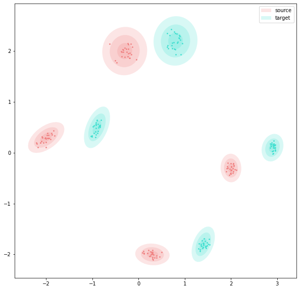
Refer to caption
Refer to caption
Refer to caption
Figure 4: The results of flowing a mixture of 4 Gaussian distributions to a mixture of 4 Gaussian distributions. We demonstrate the initialization (left), the trace of particles in first 200 steps (middle), and the results at step 1000 (right).

We test how our algorithm deals with flowing a mixture of 2 Gaussian distributions to a mixture of 4 Gaussian distributions. From the trace of first 200 steps, we demonstrate that each source Gaussian distribution splits into 2 Gaussian distributions. The source distribution and target distribution are:
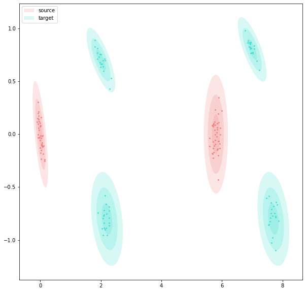
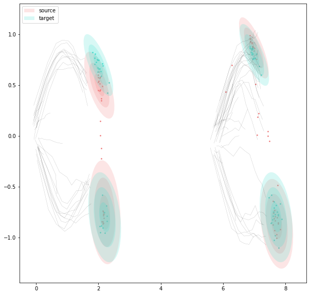
ps​(x)\displaystyle p_{s}(x) =12​𝒩​((0.00.0),(0.18−0.24−0.240.70))+12​𝒩​((5.80.0),(0.440.000.000.87))\displaystyle=\frac{1}{2}\mathcal{N}\left(\begin{pmatrix}0.0\\ 0.0\end{pmatrix},\begin{pmatrix}0.18&-0.24\\ -0.24&0.70\end{pmatrix}\right)+\frac{1}{2}\mathcal{N}\left(\begin{pmatrix}5.8\\ 0.0\end{pmatrix},\begin{pmatrix}0.44&0.00\\ 0.00&0.87\end{pmatrix}\right)
pt​(x)\displaystyle p_{t}(x) =14​𝒩​((2.00.7),(0.63−0.30−0.300.26))+14​𝒩​((2.2−0.8),(0.77−0.18−0.180.55))\displaystyle=\frac{1}{4}\mathcal{N}\left(\begin{pmatrix}2.0\\ 0.7\end{pmatrix},\begin{pmatrix}0.63&-0.30\\ -0.30&0.26\end{pmatrix}\right)+\frac{1}{4}\mathcal{N}\left(\begin{pmatrix}2.2\\ -0.8\end{pmatrix},\begin{pmatrix}0.77&-0.18\\ -0.18&0.55\end{pmatrix}\right)
+14​𝒩​((7.00.8),(0.63−0.30−0.300.26))+14​𝒩​((7.7−0.8),(0.77−0.18−0.180.55))\displaystyle+\frac{1}{4}\mathcal{N}\left(\begin{pmatrix}7.0\\ 0.8\end{pmatrix},\begin{pmatrix}0.63&-0.30\\ -0.30&0.26\end{pmatrix}\right)+\frac{1}{4}\mathcal{N}\left(\begin{pmatrix}7.7\\ -0.8\end{pmatrix},\begin{pmatrix}0.77&-0.18\\ -0.18&0.55\end{pmatrix}\right)
Refer to caption
Refer to caption
Refer to caption
Figure 5: The results of flowing a mixture of 2 Gaussian distributions to a mixture of 4 Gaussian distributions. We demonstrate the initialization (left), the trace of particles in first 200 steps (middle), and the results at step 2400 (right). We use method in Section B.3 to relabel the flowed samples and the labels correspond to their positional belongings correctly.

B.5 Implementation Details

Our algorithms and experiments are implemented in PyTorch. The *NIST images are resized to 20×2020\times 20, thus the feature space is of dimension m=400m=400. The SVHN and Tiny ImageNet images are of size 3×64×643\times 64\times 64. The classifiers for *NIST datasets are of LeNet-5 architecture. The classifiers for SVHN and Tiny ImageNet are of a ResNet-18 network. For the experiments in Figure 3, we train the classifiers with the set of data 10 epochs with Adam optimizer and learning rate 2×10⁻³²\times 10^{-3}.

When flowing images in *NIST datasets and flowing a mixture of Gaussians, we use the parameters and methods described in Table 2. As we tune the parameters, we notice the algorithm converges with a range of parameters and we report one setting in Table 2.

SVHN&TIN *NIST Gaussian (Figure 4) Gaussian (Figure 5)
α\alpha 0.002 0.001 0.3 0.3
β\beta 0.01 0.002 0.15 0.1
γ\gamma 1.0 100 1.0 0.5
initial sτs_{\tau} 1.0 0.3 0.05 0.03
noise level 0.1 0.01 0 0.1
TT 6000 150 2000 2500
Optimizer RMSprop Hinton et al. 2012 RMSprop RMSprop RMSprop
Table 2: Parameters and Optimizer

Our method assumes images of each class form one Gaussian distribution. In reality, the data can be a mixture of Gaussian. To satisfy the Gaussianity assumption, in the preprocessing step, we use a clustering method (kk-nearest neighbors) and pick only data from one mode for each class. As a consequence, the data used in the experiment satisfies the conditional Gaussian assumption. For example, the images of the digit 1 can have two modes: slanted left or slanted right. In this case, we can generate two labels (1L, 1R), and the methodology developed in this paper can be applied in a straightforward manner. When testing our transfer learning scheme, we apply the same clustering method on the test dataset, so our test set is within the same mode as our training set.

We store the preprocessed data and apply dimension reduction method on the data’s means and covariance matrices, so the Lyapunov equation is much faster to solve. We use the cluster’s mean and covariance matrix to approximate the 1-shot and 5-shor data’s mean and covariance matrix. In 1-shot learning, the covariance matrix is an identity matrix. All the code and data are available in the supplementary file. We use kk-nearest neighbors algorithm to solve the labels of the flowed data, as it performs better with the noisy scheme.

B.6 Additional Results on *NIST Datasets

We conduct additional experiments of flowing between KMNIST and FashionMNIST datasets. The results of our flows are illustrated in the same fashion as Figure 2 and are in the supplementary folder. In each subfigure, each column represents a snapshot of a certain time-step and the samples flow from the source (left) to the target (right). To check if the algorithm is converging, we compute the MMD between the source dataset and the target dataset. Figure 6 is an example of MMD decreasing in transferring the *NIST datasets:

Refer to caption
Figure 6: MMD keeps decreasing as we flow the samples from the source domain to the target domain

From FashionMNIST dataset to KMNIST dataset and from KMNIST dataset to FashionMNIST dataset, we also conduct transfer learning experiments. We use the same model architecture and training settings as in Fig. 3. We illustrate the accuracy and error bars of the 1-shot learning and 5-shot learning in Fig. 8. Our flowed samples (STS_{T}) increase the accuracy of the transferred classifiers in both 1-shot and 5-shot learning.

Refer to caption
Figure 7: Average target domain accuracy on the test split for transfer learning with one-shot (left) and five-shot (right). Results are taken over 10 independent replications, and the range of accuracy is displayed by the error bars.

B.7 Transfer Learning Results on SVHN and Tiny ImageNet

We run the same transfer learning experiments as section 5.1 on SVHN and Tiny ImageNet datasets and we report the accuracy on the test split33 3 The Tiny ImageNet dataset does not have labels for the test split, so we use the validation split.. From the results, we can see STS_{T} always improve the accuracy.

On the higher-dimensional data, it is a lot more difficult to train a strong classifier from only 1 or 5 samples each class, so the accuracy is not so high compared to the *NIST datasets. Another reason is there are only 50 samples in each class of the validation dataset of Tiny ImageNet, so the number of test samples might be too small.

Refer to caption
Figure 8: Average target domain accuracy on the test split for transfer learning with one-shot (left) and five-shot (right). Results are taken over 10 independent replications, and the range of accuracy is displayed by the error bars. The 𝟏\bm{1} and 𝟓\bm{5} in the parenthesis mean 1-shot and 5-shot transfer learning respectively.

B.8 Comparison with baseline

We compare with Alvarez-Melis and Fusi 2021’s approach as the baseline. We adopted the same values of parameters (number of steps, step size) from the paper of Alvarez-Melis and Fusi 2021 and experimented with different values of entropy regularization λ\lambda. Entropy regularization λ\lambda is a hidden parameter in their code and they reported using the value of λ=100\lambda=100 in transfer learning experiments. Also, we experimented with different methods in their code and found that “xyaugm” gives the best qualitative gradient flow results.

We test their algorithm using the same transfer learning setting as ours (using the same clustered data as our experiments), see Table 3 and Table 5 for results. The results show that their method doesn’t improve the classification accuracy after adding the transferred data STS_{T}, if we compare the accuracy D∪STD\cup S_{T} and P∪D∪STP\cup D\cup S_{T} with DD and P∪DP\cup D correspondingly.

Accuracy D∪STD\cup S_{T} P∪D∪STP\cup D\cup S_{T}
λ=0.001\lambda=0.001 0.1941 0.2478
λ=0.01\lambda=0.01 0.1175 0.2998
λ=1.0\lambda=1.0 0.1739 0.2951
λ=100\lambda=100 0.2093 0.3025
Table 3: KMNIST →\shortrightarrow MNIST
Accuracy D∪STD\cup S_{T} P∪D∪STP\cup D\cup S_{T}
λ=0.001\lambda=0.001 0.4488 0.3083
λ=0.01\lambda=0.01 0.3915 0.2897
λ=1.0\lambda=1.0 0.5268 0.4627
λ=100\lambda=100 0.2917 0.3307
Table 4: FMNIST →\shortrightarrow MNIST

For runtime comparison, the default device for Alvarez-Melis and Fusi 2021’s code is on the CPU. As we run their code on the GPU, the kernel crashed without giving any informative errors. Thus, we will compare our codes’ runtime per step on the CPU. While our approach takes about 0.5120.512 second, the approach in Alvarez-Melis and Fusi 2021 requires 74.7874.78 seconds.

B.9 Comparison with Mixup Method

We run mixup augmentation on F→\shortrightarrowM, K→\shortrightarrowM, M→\shortrightarrowF, and M→\shortrightarrowK on the same one-shot learning setting and same data as ours using the method in Zhang et al. 2017 with α=0.2\alpha=0.2 (suggested by Zhang et al. 2017). The results are in Table 5. When comparing DD with D∪STD\cup S_{T} and P∪DP\cup D with P∪D∪STP\cup D\cup S_{T}, the added mixup samples (STS_{T}) decrease the accuracy. A reason could be that there are too few examples in the target domain, thus mixup does not add much complexity to the target domain. The mixup experiments in [A] show improvements <1%<1\%, which is much smaller than ours in Fig.3.

Last, we want to emphasize that our gradient flow method aims to increase the number of samples of one distribution, so our method is a complement to augmentation methods.Both gradient flow and augmentation methods are applied in practice at the same time.

Training Data F→\shortrightarrowM K→\shortrightarrowM M→\shortrightarrowF M→\shortrightarrowK
DD 0.524 0.529 0.506 0.242
D∪STD\cup S_{T} 0.488 0.458 0.472 0.141
PP 0.097 0.033 0.037 0.089
P∪DP\cup D 0.510 0.543 0.541 0.140
P∪D∪STP\cup D\cup S_{T} 0.467 0.363 0.494 0.120
Table 5: FMNIST →\shortrightarrow MNIST

B.10 Comparison with Traditional Augmentation Methods

We conduct the traditional data augmentation methods, including random rotation and Gaussian noise, on the datasets and compare the classification accuracy with our method. The random rotation is from 0 to 90 degrees. The Gaussian noise is with kernel size (5,9) and standard deviation 0.1 and 5. All the comparison results are in Table 6–9.

Through this experiment, we show that using random rotation to augment the dataset does not improve accuracy much and sometimes even decreases the accuracy in all of the eight transfer learning settings. We note that (DD, PP, P∪DP\cup D) are settings without augmentation while (D∪STD\cup S_{T}, P∪D∪STP\cup D\cup S_{T}) are settings with augmentation. Comparing with the results of our proposed gradient flow approach in Figure 3, augmentation (by random rotation) has much lower performances than ours.

Accuracy F→MF\rightarrow M K→MK\rightarrow M M→FM\rightarrow F M→KM\rightarrow K
DD 0.535 0.512 0.483 0.240
D∪STD\cup S_{T} 0.542 0.498 0.489 0.164
PP 0.097 0.033 0.037 0.089
P∪DP\cup D 0.510 0.543 0.541 0.140
P∪D∪STP\cup D\cup S_{T} 0.551 0.581 0.454 0.124
Table 6: 1-shot learning augmented with random rotation
Accuracy F→MF\rightarrow M K→MK\rightarrow M M→FM\rightarrow F M→KM\rightarrow K
DD 0.788 0.837 0.519 0.234
D∪STD\cup S_{T} 0.569 0.545 0.490 0.174
PP 0.097 0.033 0.037 0.089
P∪DP\cup D 0.772 0.763 0.581 0.178
P∪D∪STP\cup D\cup S_{T} 0.738 0.768 0.593 0.199
Table 7: 5-shot learning augmented with random rotation
Accuracy F→MF\rightarrow M K→MK\rightarrow M M→FM\rightarrow F M→KM\rightarrow K
DD 0.524 0.529 0.506 0.242
D∪STD\cup S_{T} 0.512 0.494 0.452 0.167
PP 0.097 0.033 0.037 0.089
P∪DP\cup D 0.510 0.543 0.541 0.140
P∪D∪STP\cup D\cup S_{T} 0.557 0.590 0.454 0.127
Table 8: 1-shot learning augmented with random Gaussian noise
Accuracy F→MF\rightarrow M K→MK\rightarrow M M→FM\rightarrow F M→KM\rightarrow K
DD 0.827 0.824 0.549 0.265
D∪STD\cup S_{T} 0.792 0.803 0.734 0.320
PP 0.097 0.032 0.037 0.089
P∪DP\cup D 0.779 0.764 0.581 0.178
P∪D∪STP\cup D\cup S_{T} 0.832 0.797 0.729 0.258
Table 9: 5-shot learning augmented with random Gaussian noise

We show that adding Gaussian noise improves the accuracy in some settings, for example, M→\rightarrowF and M→\rightarrowK in 5-shot, but decreases accuracy in many settings. Our gradient flow method improves the accuracy in all the settings when we compare the accuracy without STS_{T} and with STS_{T}.

Finally, we again note that those simple augmentations, for example (adding Gaussian noise or using random rotation which are designed onto the target dataset) can be used as a complement to the gradient flow method, which transfers data from the source dataset to the target dataset.

B.11 Random Gaussian Noise to MNIST

In this section, we conduct an experiment that transfers from random noise vectors to MNIST images. The noise vectors are independently drawn from the normal distribution. Thus, the mean of the noise vectors is a zero vector and the covariance matrix is an identity matrix. From this experiment, we want to show that our method can transfer from any distribution to the target distribution.

Refer to caption
Figure 9: Our method successfully transfers from random noise vectors to MNIST images.

B.12 Evaluation Metric by SSIM and Optimal Transport

We construct a new measure that connects a human perception distance and optimal transport to measure the distance between the distribution of transferred samples and the distribution of target samples.

The target data consists of MM samples (x¯j,y¯j)j=1M(\bar{x}_{j},\bar{y}_{j})_{j=1}^{M}, and the generated data consists of NN samples (xiT,yiT)i=1N(x_{i}^{T},y_{i}^{T})_{i=1}^{N}. We use the structural similarity index measure (SSIM) wang2004image to measure image similarity between the generated images and the target images. SSIM measures the similarity between two grayscale images. SSIM is between 0 and 1, and SSIM=1\mathrm{SSIM}=1 means that the two images are identical. Thus, we define a SSIM-based cost to construct a matrix C∈ℝN×MC\in\mathbb{R}^{N\times M}: Ci​j=1−SSIM(xiT,x¯j),for i=1,…,N;j=1,…,M.C_{ij}=1-\mathrm{SSIM}(x_{i}^{T},\bar{x}_{j}),\text{for }i=1,\ldots,N;\penalty\ j=1,\ldots,M.

We use the matrix CC as a ground transportation cost and solve the Earth Mover Distance problem rubner1998metric; rubner2000earth to obtain the Wasserstein distance between target image and generated image distributions, which are 1N​∑i=1Nδ(xiT,yiT)\frac{1}{N}\sum_{i=1}^{N}\delta_{(x_{i}^{T},y_{i}^{T})}and 1M​∑j=1Mδ(x¯j,y¯j).\frac{1}{M}\sum_{j=1}^{M}\delta_{(\bar{x}_{j},\bar{y}_{j})}. We compute the distance in 1-shot FashionMNIST to MNIST experiment and Figure 10 plots the distance of each class over 10 independent runs. The plot shows our algorithm successfully decreases the Wasserstein distance between the distribution of generated images and the target distribution during each step.

Refer to caption
Figure 10: This plots the OT_SSIM distance between the distribution of transferred images and of the target images over 140 steps. The distance decreases as we flow the samples from the source domain to the target domain for every class.