跳到论文正文
W Papers独立论文阅读器 arXiv:2301.13548 论文正文 计算阅读时间 · 0%
引用这篇论文根据当前论文元数据生成,正式投稿前建议核对。


License: arXiv.org perpetual non-exclusive license
arXiv:2301.13548v1 [math.NA] 31 Jan 2023

Structure-preserving eigenvalue modification of symplectic matrices and matrix pencils

Abstract

A famous theorem by R. Brauer shows how to modify a single eigenvalue of a matrix AA by a rank-one update without changing the remaining eigenvalues. A generalization of this theorem (due to R. Rado) is used to change a pair of eigenvalues λ,1/λ\lambda,1/\lambda of a symplectic matrix SS in a structure-preserving way to desired target values μ,1/μ\mu,1/\mu. Universal bounds on the relative distance between SS and the newly constructed symplectic matrix S^\hat{S} with modified spectrum are given. The eigenvalues Segre characteristics of S^\hat{S} are related to those of SS and a statement on the eigenvalue condition numbers of S^\hat{S} is derived. The main results are extended to matrix pencils.

1. Introduction

In numerical linear algebra and matrix analysis one occasionally encounters the necessity of modifying special eigenvalues of a matrix without altering its remaining eigenvalues. Techniques for changing certain eigenvalues of a matrix have, for instance, been applied to solve nonnegative inverse eigenvalue problems [13, 16] or, in form of deflation methods, to remove dominant eigenvalues in eigenvalue computations [14, Sec. 4.2]. Furthermore, the task of modifying eigenvalues of matrices is of interest in stability and feedback of linear systems [4, § 25], [3, Sec. 2.3] or for passivity and eigenvalue assignment in control design [1]. One basic result on how a single eigenvalue of a matrix may be changed without modifying any other eigenvalues is due to R. Brauer and can be found in [3, Sec. 1], [16].

Theorem 1 (Brauer).

Let A∈Mn​(ℂ)A\in\textnormal{{M}}_{n}(\mathbb{C}) have eigenvalues λ1,…,λn∈ℂ\lambda_{1},\ldots,\lambda_{n}\in\mathbb{C} and let x1∈ℂnx_{1}\in\mathbb{C}^{n} be an eigenvector for λ1\lambda_{1}. Then, for any c∈ℂnc\in\mathbb{C}^{n}, the matrix A^=A+x1​cT∈Mn​(ℂ)\hat{A}=A+x_{1}c^{T}\in\textnormal{{M}}_{n}(\mathbb{C}) has the eigenvalues λ1+cT​x1,λ2,…,λn\lambda_{1}+c^{T}x_{1},\lambda_{2},\ldots,\lambda_{n}.

This work is concerned with the purposive change of certain eigenvalues of matrices with symplectic structure. A complex 2​n×2​n2n\times 2n matrix S∈M2​n​(ℂ)S\in\textnormal{{M}}_{2n}(\mathbb{C}) is called symplectic, if11 1 Here and in the following, T denotes the transpose of a (maybe complex) matrix or vector, not its conjugate transpose.

ST​J2​n​S=J2​n=:J,where​J2​n=[0n×nIn−In0n×n].S^{T}J_{2n}S=J_{2n}=:J,\quad\textnormal{where}\;J_{2n}=\begin{bmatrix}0_{n\times n}&I_{n}\\ -I_{n}&0_{n\times n}\end{bmatrix}. (1)

Defining S⋆:=JT​ST​JS^{\star}:=J^{T}S^{T}J, we see that (1) is equivalent to S⋆​S=I2​nS^{\star}S=I_{2n}. Therefore, a symplectic matrix SS is always nonsingular and S⋆=S−1S^{\star}=S^{-1}. In consequence, as S⋆S^{\star} is similar22 2 By definition, S⋆S^{\star} is similar to STS^{T} and by the Taussky-Zassenhaus Theorem [17], STS^{T} is similar to SS. to SS, the eigenvalues of a symplectic matrices arise in pairs λj,λj−1\lambda_{j},\lambda_{j}^{-1}, j=1,…,nj=1,\ldots,n, where λj\lambda_{j} and λj−1\lambda_{j}^{-1} have the same Segre characteristic. Recall that for an eigenvalue λ\lambda of SS, its Segre characteristic is the sequence of sizes of the Jordan blocks of SS with eigenvalue λ\lambda in non-increasing order [15]. We denote the Segre characteristic of an eigenvalue by ((,,,,,))((\cdot,\ldots,\cdot)). It is now immediate that Theorem 1 can in general not be used for a structure-preserving, symplectic change of eigenvalues. In fact, for a structure-preserving eigenvalue modification, the change of λj\lambda_{j} and λj−1\lambda_{j}^{-1} must take place simultaneously.

Without any structure-preservation in mind, changing two (or more) eigenvalues simultaneously is possible with the following generalization of Theorem 1 attributed to R. Rado. It can be found in [13], see also [3, Sec. 3].

Theorem 2 (Rado).

Let A∈Mn​(ℂ)A\in\textnormal{{M}}_{n}(\mathbb{C}) have eigenvalues λ1,…,λn∈ℂ\lambda_{1},\ldots,\lambda_{n}\in\mathbb{C} and let x1,…,xk∈ℂnx_{1},\ldots,x_{k}\in\mathbb{C}^{n} be linearly independent eigenvectors for λ1,…,λk\lambda_{1},\ldots,\lambda_{k}. Set X=[x1⋯xk]∈Mn×k(ℂ)X=[\;x_{1}\;\cdots\;x_{k}\;]\in\textnormal{{M}}_{n\times k}(\mathbb{C}). Then, for any matrix C∈Mn×k​(ℂ)C\in\textnormal{{M}}_{n\times k}(\mathbb{C}), the matrix A^=A+X​CT\hat{A}=A+XC^{T} has the eigenvalues μ1,…,μk,λk+1,…,λn\mu_{1},\ldots,\mu_{k},\lambda_{k+1},\ldots,\lambda_{n}, where μj\mu_{j}, j=1,…,kj=1,\ldots,k, are the eigenvalues of Ω=diag​(λ1,…,λn)+CT​X\Omega=\textnormal{diag}(\lambda_{1},\ldots,\lambda_{n})+C^{T}X.

In this work, we investigate how Theorem 2 can be utilized to change a pair of eigenvalues λj,λj−1\lambda_{j},\lambda_{j}^{-1} of a symplectic matrix S∈M2​n​(ℂ)S\in\textnormal{{M}}_{2n}(\mathbb{C}) (or a symplectic matrix pencil) to desired target values μ,μ−1\mu,\mu^{-1} in a structure-preserving way without modifying any other eigenvalues of SS. Considering Theorem 2, the starting point of our discussion is thus the following question:

  • Let S∈M2​n​(ℂ)S\in\textnormal{{M}}_{2n}(\mathbb{C}) be symplectic with eigenvalues λ1,λ1−1\lambda_{1},\lambda_{1}^{-1}, …\ldots , λn,λn−1\lambda_{n},\lambda_{n}^{-1}, linearly independent eigenvectors x1,x2∈ℂ2​nx_{1},x_{2}\in\mathbb{C}^{2n} for λ1\lambda_{1} and λ1−1\lambda_{1}^{-1}, respectively, and X=[x1​x2]X=[\;x_{1}\;x_{2}\;]. How has C∈M2​n×2​(ℂ)C\in\textnormal{{M}}_{2n\times 2}(\mathbb{C}) to be chosen, such that S^:=S+X​CT\hat{S}:=S+XC^{T} is symplectic with eigenvalues μ,μ−1,λ2,λ2−1,…,\mu,\mu^{-1},\lambda_{2},\lambda_{2}^{-1},\ldots, λn,λn−1\lambda_{n},\lambda_{n}^{-1} for some given value μ∈ℂ∖{0}\mu\in\mathbb{C}\setminus\{0\}?

The above-mentioned problem will be discussed in Section 2. In Section 3 we investigate whether we can find an upper bound b>0b>0 that only depends on λ1,μ,x1\lambda_{1},\mu,x_{1} and x2x_{2} that assures the existence of a symplectic matrix S^∈M2​n​(ℂ)\hat{S}\in\textnormal{{M}}_{2n}(\mathbb{C}) with eigenvalues μ,μ−1,λ2,λ2−1,…,λn,λn−1\mu,\mu^{-1},\lambda_{2},\lambda_{2}^{-1},\ldots,\lambda_{n},\lambda_{n}^{-1} and relative distance ‖S^−S‖/‖S‖≤b\|\hat{S}-S\|/\|S\|\leq b. We derive distinguished matrices S^1,S^2\hat{S}_{1},\hat{S}_{2} for which such a bound bb can be neatly expressed and related to the relative change in the eigenvalue, i.e. |λ1−μ|/|λ1||\lambda_{1}-\mu|/|\lambda_{1}|. We discuss commutativity relations between SS and S^\hat{S} in Section 4.1 and characterize the Segre characteristics of the eigenvalues of S^\hat{S} in Section 4.2. The results of Section 4.1 will come in handy here to find a condition on the simultaneous diagonalizability of SS and S^\hat{S}. In Section 6 we partially extend our results from Section 2 to symplectic matrix pencils.

1.1. Notation

The set of all m×nm\times n matrices over 𝕂\mathbb{K} (where we use either 𝕂=ℂ\mathbb{K}=\mathbb{C} or 𝕂=ℝ\mathbb{K}=\mathbb{R}) is denoted by Mm×n​(𝕂)\textnormal{{M}}_{m\times n}(\mathbb{K}). Whenever n=mn=m we write Mn​(𝕂)\textnormal{{M}}_{n}(\mathbb{K}) instead of Mn×n​(ℂ)\textnormal{{M}}_{n\times n}(\mathbb{C}). For J2​n∈M2​n​(ℝ)J_{2n}\in\textnormal{{M}}_{2n}(\mathbb{R}), see (1), we simply write JJ and add the index whenever it is necessary to specify the size of JJ. The range of a matrix A∈Mm×n​(ℂ)A\in\textnormal{{M}}_{m\times n}(\mathbb{C}) is the vector space spanned by its columns and is denoted range​(A)\textnormal{range}(A). For A∈Mm×n​(ℂ)A\in\textnormal{{M}}_{m\times n}(\mathbb{C}), we denote the Moore-Penrose pseudoinverse of AA by A+A^{+}. In case m>nm>n and rank​(A)=n\textnormal{rank}(A)=n, we have A+=(AH​A)−1​AHA^{+}=(A^{H}A)^{-1}A^{H} so that A+​A=InA^{+}A=I_{n}, while for n>mn>m and rank​(A)=m\textnormal{rank}(A)=m, A+=AH​(A​AH)−1A^{+}=A^{H}(AA^{H})^{-1} yields A​A+=ImAA^{+}=I_{m}. The superscript H always denotes the conjugate transpose of a matrix or vector while T is used for the pure transposition. Whenever λ∈ℂ\lambda\in\mathbb{C} is some complex number, we denote by ℜ⁡(λ)\mathfrak{R}(\lambda) and ℑ⁡(λ)\mathfrak{I}(\lambda) its real and imaginary part, respectively. Complex conjugation of a number x=a+ı​b∈ℂx=a+\imath b\in\mathbb{C} is denoted by a bar, i.e. x¯=a−ı​b\overline{x}=a-\imath b.

2. Symplectic Eigenvalue Modification

Let S∈M2​n​(ℂ)S\in\textnormal{{M}}_{2n}(\mathbb{C}) be a symplectic matrix (see (1)) with eigenvalues λ1,λ1−1\lambda_{1},\lambda_{1}^{-1}, …\ldots, λn,λn−1\lambda_{n},\lambda_{n}^{-1} and let μ∈ℂ∖{0}\mu\in\mathbb{C}\setminus\{0\} be given. Furthermore, assume x1,x2∈ℂ2​nx_{1},x_{2}\in\mathbb{C}^{2n} are linearly independent33 3 If λ1≠λ1−1\lambda_{1}\neq\lambda_{1}^{-1}, then x1x_{1} and x2x_{2} are necessarily linear independent. Therefore, the linear independence is only a restrictive requirement if λ1=λ1−1\lambda_{1}=\lambda_{1}^{-1}, i.e. λ1=±1\lambda_{1}=\pm 1. eigenvectors of SS for λ1\lambda_{1} and λ1−1\lambda_{1}^{-1}, respectively, and define X=[x1​x2]∈M2​n×2​(ℂ)X=[\;x_{1}\;x_{2}\;]\in\textnormal{{M}}_{2n\times 2}(\mathbb{C}). In this section, our goal is to determine all possible matrices C∈M2​n×2​(ℂ)C\in\textnormal{{M}}_{2n\times 2}(\mathbb{C}) such that S^:=S+X​CT\hat{S}:=S+XC^{T} is again symplectic and has the eigenvalues μ,μ−1,λ2,λ2−1,…,λn,λn−1\mu,\mu^{-1},\lambda_{2},\lambda_{2}^{-1},\ldots,\lambda_{n},\lambda_{n}^{-1}. To this end, we will make use of Rado’s theorem and derive a structure-preserving version of Theorem 2 (see Theorem 3).

As it will become clear later, it seems appropriate to consider the situations x1T​J​x2≠0x_{1}^{T}Jx_{2}\neq 0 and x1T​J​x2=0x_{1}^{T}Jx_{2}=0 seperately. First, we assume that for the eigenvalues λ1,λ1−1\lambda_{1},\lambda_{1}^{-1} there exist eigenvectors x1,x2∈ℂ2​nx_{1},x_{2}\in\mathbb{C}^{2n} such that x1T​J​x2≠0x_{1}^{T}Jx_{2}\neq 0 (this immediately implies x1x_{1} and x2x_{2} to be linearly independent). In this case, we can assume w. l. o. g. x1T​J​x2=1x_{1}^{T}Jx_{2}=1, which can be achieved by a scaling of x1x_{1} and/or x2x_{2}. That is, we have XT​J​X=J2X^{T}JX=J_{2}. For the matrix S^:=S+X​CT\hat{S}:=S+XC^{T} to be symplectic, it has to hold that

S^T​J​S^=(S+X​CT)T​J​(S+X​CT)=J.\hat{S}^{T}J\hat{S}=\big(S+XC^{T}\big)^{T}J\big(S+XC^{T}\big)=J. (2)

Using ST​J​S=JS^{T}JS=J, (2) is equivalent to the matrix equation

C​XT​J​S+ST​J​X​CT+C​XT​J​X​CT=0CX^{T}JS+S^{T}JXC^{T}+CX^{T}JXC^{T}=0 (3)

for the unknown matrix C∈M2​n×2​(ℂ)C\in\textnormal{{M}}_{2n\times 2}(\mathbb{C}). Notice that (3) can be rewritten as

C⁡(XT​J​S+J2​CT)=−ST​J​X​CTC(X^{T}JS+J_{2}C^{T})=-S^{T}JXC^{T} (4)

using XT​J​X=J2X^{T}JX=J_{2}. Since ST​J​X∈M2​n×2​(ℂ)S^{T}JX\in\textnormal{{M}}_{2n\times 2}(\mathbb{C}) is a matrix of full rank, (4) immediately implies range​(C)⊆range​(ST​J​X)\textnormal{range}(C)\subseteq\textnormal{range}(S^{T}JX) for any solution CC. Thus, for every CC satisfying (3), there is a matrix R=[ri​j]i​j∈M2​(ℂ)R=[r_{ij}]_{ij}\in\textnormal{{M}}_{2}(\mathbb{C}) such that C=ST​J​X​RTC=S^{T}JXR^{T}. Plugging this ansatz into (3), we obtain a 2​n×2​n2n\times 2n equation for RR, namely

ST​J​X​RT​XT​J​S+ST​J​X​R​XT​JT​S+ST​J​X​RT​J2​R​XT​JT​S=0.S^{T}JXR^{T}X^{T}JS+S^{T}JXRX^{T}J^{T}S+S^{T}JXR^{T}J_{2}RX^{T}J^{T}S=0.

Replacing XT​J​SX^{T}JS by −XT​JT​S-X^{T}J^{T}S this can be rewritten as

ST​J​X​(R−RT+RT​J2​R)​XT​JT​S=0.S^{T}JX\big(R-R^{T}+R^{T}J_{2}R\big)X^{T}J^{T}S=0. (5)

Finally, we may multiply (5) with the pseudo inverses (ST​J​X)+(S^{T}JX)^{+} from the left and with (XT​JT​S)+(X^{T}J^{T}S)^{+} from the right to obtain

R−RT+RT​J2​R=0,R-R^{T}+R^{T}J_{2}R=0, (6)

which is a matrix equation for RR of size 2×22\times 2 that is equivalent to (5). As R−RTR-R^{T} and RT​J2​RR^{T}J_{2}R are both skew-symmetric, their diagonals are identically zero. Comparing the entries of R−RTR-R^{T} and RT​J2​RR^{T}J_{2}R in the (1,2) position, we obtain the condition

r12−r21+r11​r22−r12​r21=0r_{12}-r_{21}+r_{11}r_{22}-r_{12}r_{21}=0 (7)

for (6) to hold (comparing the elements in the (2,1)(2,1) position certainly gives the same condition with a minus sign). In summary, a matrix of the form S^=S+X​CT\hat{S}=S+XC^{T} is symplectic if and only if C=ST​J​X​RTC=S^{T}JXR^{T} for some matrix R=[ri​j]i​j∈M2​(ℂ)R=[r_{ij}]_{ij}\in\textnormal{{M}}_{2}(\mathbb{C}) whose entries satisfy (7).

Next, to achieve the desired eigenvalue modification, according to Theorem 2 we need to assure that the eigenvalues of

Ω:=Λ+CT​X=[λ100λ1−1]+CT​X=[λ100λ1−1]+R​XT​JT​S​X\Omega:=\Lambda+C^{T}X=\begin{bmatrix}\lambda_{1}&0\\ 0&\lambda_{1}^{-1}\end{bmatrix}+C^{T}X=\begin{bmatrix}\lambda_{1}&0\\ 0&\lambda_{1}^{-1}\end{bmatrix}+RX^{T}J^{T}SX (8)

become equal to μ\mu and μ−1\mu^{-1}. To this end, recall that S​X=X​diag​(λ1,λ1−1)SX=X\textnormal{diag}(\lambda_{1},\lambda_{1}^{-1}) (by construction of XX). Thus diag​(λ1,λ1−1)+R​XT​JT​S​X=diag​(λ1,λ1−1)−R​XT​J​X​diag​(λ1,λ1−1)\textnormal{diag}(\lambda_{1},\lambda_{1}^{-1})+RX^{T}J^{T}SX=\textnormal{diag}(\lambda_{1},\lambda_{1}^{-1})-RX^{T}JX\textnormal{diag}(\lambda_{1},\lambda_{1}^{-1}) which, since XT​J​X=J2X^{T}JX=J_{2}, yields

Ω=[λ100λ1−1]−R​J2​[λ100λ1−1]=[λ1+λ1​r12−λ1−1​r11λ1​r22λ1−1−λ1−1​r21].\Omega=\begin{bmatrix}\lambda_{1}&0\\ 0&\lambda_{1}^{-1}\end{bmatrix}-RJ_{2}\begin{bmatrix}\lambda_{1}&0\\ 0&\lambda_{1}^{-1}\end{bmatrix}=\begin{bmatrix}\lambda_{1}+\lambda_{1}r_{12}&-\lambda_{1}^{-1}r_{11}\\ \lambda_{1}r_{22}&\lambda_{1}^{-1}-\lambda_{1}^{-1}r_{21}\end{bmatrix}. (9)

The characteristic polynomial of Ω\Omega is

p⁡(z)=z2−(λ1​(1+r12)+λ1−1​(1−r21))​z+(1+r12)​(1−r21)+r11​r22,p(z)=z^{2}-\big(\lambda_{1}(1+r_{12})+\lambda_{1}^{-1}(1-r_{21})\big)z+(1+r_{12})(1-r_{21})+r_{11}r_{22},

which should, by Theorem 2, be equal to q⁡(z)=(z−μ)​(z−μ−1)=z2−(μ+μ−1)+1q(z)=(z-\mu)(z-\mu^{-1})=z^{2}-(\mu+\mu^{-1})+1 to achieve that S^\hat{S} will have the eigenvalues μ\mu and μ−1\mu^{-1}. This gives two more conditions: one the one hand λ1​(1+r12)+λ1−1​(1−r21)=μ+μ−1\lambda_{1}(1+r_{12})+\lambda_{1}^{-1}(1-r_{21})=\mu+\mu^{-1}, i.e.

λ1​r12−λ1−1​r21=(μ+μ−1)−(λ1+λ1−1).\lambda_{1}r_{12}-\lambda_{1}^{-1}r_{21}=(\mu+\mu^{-1})-(\lambda_{1}+\lambda_{1}^{-1}). (10)

One the other hand, (1+r12)​(1−r21)+r11​r22=1(1+r_{12})(1-r_{21})+r_{11}r_{22}=1. The latter condition, however, is equal to condition (7) obtained for the symplectic structure above. Thus, additionally to (7), which is required for S+X​CTS+XC^{T} to be symplectic, the equation (10) has to hold to achieve that μ,μ−1\mu,\mu^{-1} become eigenvalues of S+X​CTS+XC^{T}. In conclusion, we obtain the following version of Theorem 2 that answers the question stated in Section 1 on the eigenvalue modification for symplectic matrices.

Theorem 3.

Let S∈M2​n​(ℂ)S\in\textnormal{{M}}_{2n}(\mathbb{C}) be symplectic with eigenvalues λ1,λ1−1,λ2,λ2−1,\lambda_{1},\lambda_{1}^{-1},\lambda_{2},\lambda_{2}^{-1}, …,λn,λn−1\ldots,\lambda_{n},\lambda_{n}^{-1} and let μ∈ℂ∖{0}\mu\in\mathbb{C}\setminus\{0\} be given. Let x1,x2∈ℂ2​nx_{1},x_{2}\in\mathbb{C}^{2n} be eigenvectors for λ1\lambda_{1} and λ1−1\lambda_{1}^{-1}, respectively, normalized such that XT​J​X=J2X^{T}JX=J_{2} for X=[x1​x2]∈M2​n×2​(ℂ)X=[\;x_{1}\;x_{2}\;]\in\textnormal{{M}}_{2n\times 2}(\mathbb{C}) and set d:=(μ+μ−1)−(λ1+λ1−1)d:=(\mu+\mu^{-1})-(\lambda_{1}+\lambda_{1}^{-1}). Then the matrix

S^:=S+X​CT∈M2​n​(ℂ)\hat{S}:=S+XC^{T}\in\textnormal{{M}}_{2n}(\mathbb{C}) (11)

is symplectic and has the eigenvalues μ,μ−1,λ2,λ2−1,…,λn,λn−1\mu,\mu^{-1},\lambda_{2},\lambda_{2}^{-1},\ldots,\lambda_{n},\lambda_{n}^{-1} if and only if CT=R​XT​JT​SC^{T}=RX^{T}J^{T}S for some matrix R=[ri​j]i​j∈M2​(ℂ)R=[r_{ij}]_{ij}\in\textnormal{{M}}_{2}(\mathbb{C}) whose entries satisfy the conditions

d\displaystyle d =λ1​r12−λ1−1​r21,and\displaystyle=\lambda_{1}r_{12}-\lambda_{1}^{-1}r_{21},\;\textnormal{and} (12)
0\displaystyle 0 =r12−r21+r11​r22−r12​r21.\displaystyle=r_{12}-r_{21}+r_{11}r_{22}-r_{12}r_{21}. (13)

Notice that the matrix S^=S+X​R​XT​JT​S\hat{S}=S+XRX^{T}J^{T}S in (11) can also be expressed as S^=(I2​n+X​R​XT​JT)​S\hat{S}=(I_{2n}+XRX^{T}J^{T})S or as

S^=S+X​R​Λ−1​XT​JT\displaystyle\hat{S}=S+XR\Lambda^{-1}X^{T}J^{T} =S+X​R​[λ1−100λ1]​XT​JT\displaystyle=S+XR\begin{bmatrix}\lambda_{1}^{-1}&0\\ 0&\lambda_{1}\end{bmatrix}X^{T}J^{T} (14)

according to the relation Λ−1​XT​JT=XT​JT​S\Lambda^{-1}X^{T}J^{T}=X^{T}J^{T}S (where Λ=diag​(λ1,λ1−1)\Lambda=\textnormal{diag}(\lambda_{1},\lambda_{1}^{-1})). Furthermore, we see from (12) and (13) that there exist infinitely many possible choices for RR that realize the desired eigenvalue modification.

Next, we discuss the case that the eigenvectors x1,x2∈ℂ2​nx_{1},x_{2}\in\mathbb{C}^{2n} of the symplectic matrix SS for λ1\lambda_{1} and λ1−1\lambda_{1}^{-1}, respectively, satisfy x1T​J​x2=0x_{1}^{T}Jx_{2}=0 and how this condition effects the result from Theorem 3. To this end, first notice that a symplectic matrix S∈M2​n​(ℂ)S\in\textnormal{{M}}_{2n}(\mathbb{C}) need in fact not have eigenvectors x1,x2x_{1},x_{2} for λ1\lambda_{1} and λ1−1\lambda_{1}^{-1} that satisfy x1T​J​x2≠0.x_{1}^{T}Jx_{2}\neq 0. A situation of this kind arises for the symplectic matrix

S=[λ11000λ10000λ1−1000−λ1−2λ1−1]S=\begin{bmatrix}\lambda_{1}&1&0&0\\ 0&\lambda_{1}&0&0\\ 0&0&\lambda_{1}^{-1}&0\\ 0&0&-\lambda_{1}^{-2}&\lambda_{1}^{-1}\end{bmatrix}

and its eigenvalue λ1\lambda_{1}. The only eigenvectors for λ1\lambda_{1} and λ1−1\lambda_{1}^{-1} are e1e_{1} and e4e_{4}, respectively, and we have e1T​J4​e4=0e_{1}^{T}J_{4}e_{4}=0. Thus, Theorem 3 cannot be applied. A simple sufficient (but not necessary) criterion to assure that eigenvectors with x1T​J​x2≠0x_{1}^{T}Jx_{2}\neq 0 must exist, is that SS is a diagonalizable matrix, cf. [10, Lem. 3, Cor. 3.1] and Corollary 1 below.

Whenever x1,x2∈ℂ2​nx_{1},x_{2}\in\mathbb{C}^{2n} are eigenvectors of SS for λ1\lambda_{1} and λ1−1\lambda_{1}^{-1} with x1T​J​x2=0x_{1}^{T}Jx_{2}=0, then XT​J​X=0X^{T}JX=0 follows for X=[x1​x2]X=[\;x_{1}\;x_{2}\;]. In this case, it follows from (3) that (4) takes the form

C​XT​J​S=−ST​J​X​CT.CX^{T}JS=-S^{T}JXC^{T}.

Again we obtain range​(C)⊆range​(ST​J​X)\textnormal{range}(C)\subseteq\textnormal{range}(S^{T}JX), so there has to exist some matrix R=[ri​j]i​j∈M2​(ℂ)R=[r_{ij}]_{ij}\in\textnormal{{M}}_{2}(\mathbb{C}) such that C=ST​J​X​RTC=S^{T}JXR^{T}. However, despite the concrete form of RR, analogously to (8) we obtain

Ω=[λ00λ−1]+CT​X=[λ00λ−1]−R​XT​J​S​X=[λ00λ−1]\Omega=\begin{bmatrix}\lambda&0\\ 0&\lambda^{-1}\end{bmatrix}+C^{T}X=\begin{bmatrix}\lambda&0\\ 0&\lambda^{-1}\end{bmatrix}-RX^{T}JSX=\begin{bmatrix}\lambda&0\\ 0&\lambda^{-1}\end{bmatrix}

since S​X=X​diag​(λ,λ−1)SX=X\textnormal{diag}(\lambda,\lambda^{-1}) and XT​J​X=0X^{T}JX=0. Thus, even if RR is chosen according to (13) such that S^=S+X​R​XT​JT​S\hat{S}=S+XRX^{T}J^{T}S is symplectic, no change in the eigenvalues can be achieved. In consequence, a change of an eigenvalue pair λ1,λ1−1\lambda_{1},\lambda_{1}^{-1} of a symplectic matrix by Rado’s theorem in a structure-preserving way is only possible if there exist eigenvectors x1x_{1} and x2x_{2} for λ1\lambda_{1} and λ1−1\lambda_{1}^{-1}, respectively, such that x1T​J​x2≠0x_{1}^{T}Jx_{2}\neq 0. In the next section, we derive a universal criterion on the existence of such eigenvectors.

2.1. Applying Theorem 3: a criterion

We will now characterize those symplectic matrices S∈M2​n​(ℂ)S\in\textnormal{{M}}_{2n}(\mathbb{C}), for which an eigenvalue adjustment according to Theorem 3 is possible. The condition derived below involves the Segre characteristic of the eigenvalue λ1∈σ⁡(S)\lambda_{1}\in\sigma(S) to be modified.

First, let λ1∈σ⁡(S)\lambda_{1}\in\sigma(S) and S​x1=λ1​x1Sx_{1}=\lambda_{1}x_{1} and S​x2=λ1−1​x2Sx_{2}=\lambda_{1}^{-1}x_{2}. Now suppose at least one of both vectors, e.g. x1x_{1}, belongs to a nontrivial44 4 By nontrivial, we mean a Jordan chain of length ≥2\geq 2 while a trivial Jordan chain refers to a chain of length one. Jordan chain, that is, there is some z∈ℂ2​nz\in\mathbb{C}^{2n} such that (S−λ1​I2​n)​z=x1(S-\lambda_{1}I_{2n})z=x_{1} (and possibly more generalized eigenvectors beside zz). Then we have

x1T​J​x2=((S−λ1​I2​n)​z)T​J​x2\displaystyle x_{1}^{T}Jx_{2}=\big((S-\lambda_{1}I_{2n})z\big)^{T}Jx_{2} =zT​ST​J​x2−λ1​zT​J​x2\displaystyle=z^{T}S^{T}Jx_{2}-\lambda_{1}z^{T}Jx_{2} (15)
=zT​J​JT​ST​J​x2−λ1​zT​J​x2\displaystyle=z^{T}JJ^{T}S^{T}Jx_{2}-\lambda_{1}z^{T}Jx_{2}
=zT​J​S−1​x2−λ1​zT​J​x2\displaystyle=z^{T}JS^{-1}x_{2}-\lambda_{1}z^{T}Jx_{2}
=λ1​zT​J​x2−λ1​zT​J​x2=0\displaystyle=\lambda_{1}z^{T}Jx_{2}-\lambda_{1}z^{T}Jx_{2}=0

as JT​ST​J=S⋆=S−1J^{T}S^{T}J=S^{\star}=S^{-1} and S−1​x2=λ1​x2S^{-1}x_{2}=\lambda_{1}x_{2}. In consequence, x1T​J​x2=0x_{1}^{T}Jx_{2}=0 whenever x1,x2x_{1},x_{2} are eigenvectors of SS for λ1\lambda_{1} and λ1−1\lambda_{1}^{-1}, respectively, and at least one of them belongs to a nontrivial Jordan chain. In other words, we may have x1T​J​x2≠0x_{1}^{T}Jx_{2}\neq 0 only in case both x1x_{1} and x2x_{2} belong to trivial Jordan chains. Next, we show that in case x1x_{1} belongs to a trivial Jordan chain there must exist x2x_{2} (also from a trivial Jordan chain) such that x1T​J​x2≠0x_{1}^{T}Jx_{2}\neq 0.

To this end, assume that λ1∈ℂ\lambda_{1}\in\mathbb{C} is an eigenvalue of the symplectic matrix S∈M2​n​(ℂ)S\in\textnormal{{M}}_{2n}(\mathbb{C}) with p≥1p\geq 1 ones in its Segre characteristic (that is, there are pp Jordan blocks of size 1×11\times 1, i.e. pp trivial Jordan chains, and possibly other Jordan blocks of size ≥2\geq 2). Then there exists a matrix F∈M2​n​(ℂ)F\in\textnormal{{M}}_{2n}(\mathbb{C}) transforming SS to the following Jordan form

F−1​S​F=:G=[λ1⋱λ100G^]F^{-1}SF=:G=\begin{bmatrix}\begin{array}[]{c|c}\begin{array}[]{ccc}\lambda_{1}&&\\ &\ddots&\\ &&\lambda_{1}\end{array}&0\\ \hline\cr 0&\hat{G}\end{array}\end{bmatrix} (16)

where the upper-left block is λ1​Ip\lambda_{1}I_{p} and G^\hat{G} contains all other Jordan blocks (note that there might also be other Jordan blocks for λ1\lambda_{1} of size ≥2\geq 2 contained in G^\hat{G}). Now define

x1:=F​e1andf~H:=e1T​F−1.x_{1}:=Fe_{1}\quad\textnormal{and}\quad\tilde{f}^{H}:=e_{1}^{T}F^{-1}. (17)

Then x1x_{1} is a right eigenvector of SS for λ1\lambda_{1} (S​x1=λ1​x1Sx_{1}=\lambda_{1}x_{1}) and f~\tilde{f} is a left eigenvector of SS for λ1\lambda_{1} (f~H​S=λ1​f~H\tilde{f}^{H}S=\lambda_{1}\tilde{f}^{H}). Certainly, f~H​x1=1\tilde{f}^{H}x_{1}=1. Now we define x2T:=f~H​Jx_{2}^{T}:=\tilde{f}^{H}J. Then we have

f~H​S=λ1​f~H\displaystyle\tilde{f}^{H}S=\lambda_{1}\tilde{f}^{H} ⇔x2T​JT​S=λ1​x2T​JT\displaystyle\Leftrightarrow\;x_{2}^{T}J^{T}S=\lambda_{1}x_{2}^{T}J^{T} (18)
⇔x2T​JT​S​J=λ1​x2T\displaystyle\Leftrightarrow\;x_{2}^{T}J^{T}SJ=\lambda_{1}x_{2}^{T}
⇔x2T​S−T=λ1​x2T⇔S​x2=λ1−1​x2.\displaystyle\Leftrightarrow\;x_{2}^{T}S^{-T}=\lambda_{1}x_{2}^{T}\;\Leftrightarrow\;Sx_{2}=\lambda_{1}^{-1}x_{2}.

It follows that x2x_{2} is an eigenvector of SS for λ1−1\lambda_{1}^{-1}. Now we obtain

x1T​J​x2=x2T​JT​x1=f~H​x1=1≠0.x_{1}^{T}Jx_{2}=x_{2}^{T}J^{T}x_{1}=\tilde{f}^{H}x_{1}=1\neq 0.

In conclusion, for any eigenvector x1x_{1} of SS for λ1\lambda_{1} belonging to a trivial Jordan chain, there always exists an eigenvector x2x_{2} of SS for λ1−1\lambda_{1}^{-1} such that x1T​J​x2≠0.x_{1}^{T}Jx_{2}\neq 0. Recall from our observation (15) above, that x2x_{2} must also be a vector from a trivial Jordan chain. We conclude our findings in the following theorem.

Theorem 4.

Let S∈M2​n​(ℂ)S\in\textnormal{{M}}_{2n}(\mathbb{C}) be symplectic with λ1∈σ⁡(S)\lambda_{1}\in\sigma(S) and let μ∈ℂ∖{0}\mu\in\mathbb{C}\setminus\{0\} be given. Then Theorem 3 is applicable to SS for λ1\lambda_{1} and μ\mu, i.e. there exist eigenvectors x1,x2∈ℂ2​nx_{1},x_{2}\in\mathbb{C}^{2n} for λ1\lambda_{1} and λ1−1\lambda_{1}^{-1}, respectively, with x1T​J​x2≠0x_{1}^{T}Jx_{2}\neq 0, if and only if the Segre characteristic of SS for λ1\lambda_{1} contains a one, that is, it has the form ((,,,,,,,,,))((\star,\star,\cdots,\star,1)). In particular, eigenvectors x1x_{1} for λ1\lambda_{1} and x2x_{2} for λ1−1\lambda_{1}^{-1} with x1T​J​x2≠0x_{1}^{T}Jx_{2}\neq 0 always belong to trivial Jordan chains of SS.

Do not overlook that Theorem 4 applies also for λ1=λ1−1\lambda_{1}=\lambda_{1}^{-1}, i.e. λ1=±1\lambda_{1}=\pm 1. In this case λ1∈σ⁡(S)\lambda_{1}\in\sigma(S) necessarily has an even multiplicity and an even number of Jordan blocks of the same size, so a Segre characteristic of the form ((,,,,,,,,,))((\star,\star,\cdots,\star,1)) implies that there appears at least another one, i.e. ((,,,,,,,,,,,))((\star,\star,\cdots,\star,1,1)). Then the reasoning in (16), (17) and (18) applies in the same way. If SS is diagonalizable, the Segre characteristic of SS for any eigenvalue λj∈σ⁡(S)\lambda_{j}\in\sigma(S) consists only of ones. So we immediately obtain the following corollary.

Corollary 1.

Let S∈M2​n​(ℂ)S\in\textnormal{{M}}_{2n}(\mathbb{C}) be symplectic with λ1∈σ⁡(S)\lambda_{1}\in\sigma(S) and let μ∈ℂ∖{0}\mu\in\mathbb{C}\setminus\{0\} be given. Then Theorem 3 is applicable to SS for λ1\lambda_{1} and μ\mu if SS is diagonalizable.

3. Bounding the relative change

Let S∈M2​n​(ℂ)S\in\textnormal{{M}}_{2n}(\mathbb{C}) be symplectic. For the matrix S^=S+X​R​XT​JT​S\hat{S}=S+XRX^{T}J^{T}S in (11) we immediately obtain a bound on its (absolute or relative) change in norm with respect to SS. That is,

‖S−S^‖≤‖R‖|X|‖XT‖​‖S‖and‖S−S^‖‖S‖≤‖R‖​‖X‖​‖XT‖\|S-\hat{S}\|\leq\|R\|\|X\|\|X^{T}\|\|S\|\quad\textnormal{and}\quad\frac{\|S-\hat{S}\|}{\|S\|}\leq\|R\|\|X\|\|X^{T}\| (19)

hold for any submultiplicative and unitarily invariant matrix norm ∥⋅∥\|\cdot\|. In this section, we intend to derive explicit bounds of the relative distance between SS and S^\hat{S} for certain choices of R=[ri​j]i​j∈M2​(ℂ)R=[r_{ij}]_{ij}\in\textnormal{{M}}_{2}(\mathbb{C}). To this end, we assume ∥⋅∥=∥⋅∥F\|\cdot\|=\|\cdot\|_{F} so that ‖X‖F=‖XT‖F\|X\|_{F}=\|X^{T}\|_{F} holds and the upper bound in (19) reduces to ‖R‖F​‖X‖F2\|R\|_{F}\|X\|_{F}^{2}.

To bound the relative change ‖S^−S‖F/‖S‖F\|\hat{S}-S\|_{F}/\|S\|_{F} with respect to SS consider again (12) and (13). The solution set to (12) is an affine subspace of ℂ2\mathbb{C}^{2} and all solutions may be parameterized as

r12=η​λ1−1,r21=−λ1​d+η​λ1,η∈ℂ.r_{12}=\eta\lambda_{1}^{-1},\qquad r_{21}=-\lambda_{1}d+\eta\lambda_{1},\qquad\eta\in\mathbb{C}. (20)

Plugging these expressions for r12r_{12} and r21r_{21} into (13) yields a polynomial in η\eta, i.e.

p⁡(η)=−η2+η⁡(λ1−1+d−λ1)+d​λ1+r11​r22.p(\eta)=-\eta^{2}+\eta\left(\lambda_{1}^{-1}+d-\lambda_{1}\right)+d\lambda_{1}+r_{11}r_{22}. (21)

Thus, depending on r11r_{11} and r22r_{22} (which can both be arbitrary), in (21) there are always two solutions η1,η2∈ℂ\eta_{1},\eta_{2}\in\mathbb{C} of p⁡(η)=0p(\eta)=0 and, in consequence, two matrices

R(ηj,r11,r22):=[r11ηj​λ1−1λ1​(ηj−d)r22],j=1,2,R(\eta_{j},r_{11},r_{22}):=\begin{bmatrix}r_{11}&\eta_{j}\lambda_{1}^{-1}\\ \lambda_{1}(\eta_{j}-d)&r_{22}\end{bmatrix},\quad j=1,2, (22)

so that their entries satisfy (12) and (13).

To find some R∈M2​(ℂ)R\in\textnormal{{M}}_{2}(\mathbb{C}) that yields a small norm ‖R‖F\|R\|_{F} and thus a small bound in (19), it seems natural to consider the case r11​r22=0r_{11}r_{22}=0, in particular r11=r22=0r_{11}=r_{22}=055 5 Certainly, choosing r11=0r_{11}=0 and r22≠0r_{22}\neq 0 gives the same roots of p⁡(η)=0p(\eta)=0 in (21), and thus the same values for r12r_{12} and r21r_{21}, but a larger Frobenius norm of RR than choosing r11=r22=0r_{11}=r_{22}=0.. The two possible roots of p⁡(η)p(\eta) for r11​r22=0r_{11}r_{22}=0 are η1=μ−λ1\eta_{1}=\mu-\lambda_{1} and η2=μ−1−λ1\eta_{2}=\mu^{-1}-\lambda_{1}. The matrices R1:=R⁡(η1,0,0)R_{1}:=R(\eta_{1},0,0) and R2:=R⁡(η2,0,0)R_{2}:=R(\eta_{2},0,0) that arise according to (22) are thus given by

R1=[0λ1−1​(μ−λ1)μ−1​(μ−λ1)0],R2=[0μ−1​(λ1−1−μ)λ1​(λ1−1−μ)0].R_{1}=\begin{bmatrix}0&\lambda_{1}^{-1}(\mu-\lambda_{1})\\ \mu^{-1}(\mu-\lambda_{1})&0\end{bmatrix},\quad R_{2}=\begin{bmatrix}0&\mu^{-1}(\lambda_{1}^{-1}-\mu)\\ \lambda_{1}(\lambda_{1}^{-1}-\mu)&0\end{bmatrix}. (23)

Using R1R_{1} and R2R_{2} in (23), explicit bounds can be found on ‖S^−S‖F/‖S‖F\|\hat{S}-S\|_{F}/\|S\|_{F}. According to (19) and (23) such a bound b≥0b\geq 0 only depends on λ1\lambda_{1}, μ\mu and the eigenvectors of SS for λ1\lambda_{1} and λ1−1\lambda_{1}^{-1} and guarantees the existence of a symplectic matrix S^∈M2​n​(ℂ)\hat{S}\in\textnormal{{M}}_{2n}(\mathbb{C}) that solves the problem from Section 1 with ‖S^−S‖F/‖S‖F≤b\|\hat{S}-S\|_{F}/\|S\|_{F}\leq b. To formulate these bounds, we impose a condition on XX to estimate ‖X‖F\|X\|_{F} without computing the norm. In particular, we assume the eigenvectors x1,x2∈ℂ2​nx_{1},x_{2}\in\mathbb{C}^{2n} of SS for λ1\lambda_{1} and λ1−1\lambda_{1}^{-1}, respectively, to be normalized, i.e. ‖x1‖2=‖x2‖2=1\|x_{1}\|_{2}=\|x_{2}\|_{2}=1 and X∈M2​n×2​(ℂ)X\in\textnormal{{M}}_{2n\times 2}(\mathbb{C}) to be of the form

X=1x1T​J​x2​[x1x2].X=\frac{1}{\sqrt{x_{1}^{T}Jx_{2}}}\begin{bmatrix}x_{1}&x_{2}\end{bmatrix}. (24)

Then XT​J​X=J2X^{T}JX=J_{2} holds and it follows that

‖X‖F2=|1x1T​J​x2|2​‖[x1x2]‖F2=1|x1T​J​x2|​‖[x1x2]‖F2=2|x1T​J​x2|\|X\|_{F}^{2}=\left|\frac{1}{\sqrt{x_{1}^{T}Jx_{2}}}\right|^{2}\left\|\begin{bmatrix}x_{1}&x_{2}\end{bmatrix}\right\|_{F}^{2}=\frac{1}{|x_{1}^{T}Jx_{2}|}\left\|\begin{bmatrix}x_{1}&x_{2}\end{bmatrix}\right\|_{F}^{2}=\frac{2}{|x_{1}^{T}Jx_{2}|} (25)

The value 1/|x1T​J​x2|1/|x_{1}^{T}Jx_{2}| has a nice interpretation whenever λ1\lambda_{1} is a simple eigenvalue of SS and ‖x1‖2=‖x2‖2=1\|x_{1}\|_{2}=\|x_{2}\|_{2}=1 holds. To see this, recall that, whenever A∈Mn​(ℂ)A\in\textnormal{{M}}_{n}(\mathbb{C}) has a simple eigenvalue λ∈ℂ\lambda\in\mathbb{C} (i.e. its algebraic multiplicity equals one), then

κ⁡(A,λ):=‖u‖2​‖v‖2|vH​u|\kappa(A,\lambda):=\frac{\|u\|_{2}\|v\|_{2}}{|v^{H}u|}

is called its condition number, where u∈ℂ2​nu\in\mathbb{C}^{2n} and v∈ℂ2​nv\in\mathbb{C}^{2n} are right and left eigenvectors of AA for λ\lambda (i.e. A​u=λ​uAu=\lambda u and vH​A=λ​vHv^{H}A=\lambda v^{H}). It is a measure on how sensitive λ\lambda reacts to small changes in the matrix AA, see [14, Sec. 3.3]. As we have seen in (18) above, (x2T​JT)​S=λ1​(x2T​JT)(x_{2}^{T}J^{T})S=\lambda_{1}(x_{2}^{T}J^{T}) whenever x2x_{2} satisfies S​x2=λ1−1​x2Sx_{2}=\lambda_{1}^{-1}x_{2}. Thus, for simple λ1\lambda_{1} (which implies that λ1−1\lambda_{1}^{-1} is simple as well) we can choose u=x1u=x_{1} and vH=x2T​JTv^{H}=x_{2}^{T}J^{T} so that

κ⁡(S,λ1)=‖u‖2​‖v‖2|vH​u|=‖x1‖2​‖J​x¯2‖2|x2T​JT​x1|=1|x1T​J​x2|\kappa(S,\lambda_{1})=\frac{\|u\|_{2}\|v\|_{2}}{|v^{H}u|}=\frac{\|x_{1}\|_{2}\|J\overline{x}_{2}\|_{2}}{|x_{2}^{T}J^{T}x_{1}|}=\frac{1}{|x_{1}^{T}Jx_{2}|}

since ‖x1‖2=1\|x_{1}\|_{2}=1 and ‖J​x¯2‖2=‖x¯2‖2=‖x2‖2=1\|J\overline{x}_{2}\|_{2}=\|\overline{x}_{2}\|_{2}=\|x_{2}\|_{2}=1. We can now formulate the following theorem which follows directly from the bound in (19), the observation in (25) and the Frobenius norms of the matrices R1,R2R_{1},R_{2} in (23).

Theorem 5.

Let S∈M2​n​(ℂ)S\in\textnormal{{M}}_{2n}(\mathbb{C}) be symplectic with λ1,λ1−1∈σ⁡(S)\lambda_{1},\lambda_{1}^{-1}\in\sigma(S) and let μ∈ℂ∖{0}\mu\in\mathbb{C}\setminus\{0\} be given. Let x1,x2∈ℂ2​nx_{1},x_{2}\in\mathbb{C}^{2n} be normalized eigenvectors for λ1\lambda_{1} and λ1−1\lambda_{1}^{-1}, respectively, and X∈M2​n×2​(ℂ)X\in\textnormal{{M}}_{2n\times 2}(\mathbb{C}) as in (24). Define

Φ:=2|x1T​J​x2|(=2​κ​(S,λ1)​if λ1 is simple).\Phi:=\frac{2}{|x_{1}^{T}Jx_{2}|}\;\big(=2\kappa(S,\lambda_{1})\;\textnormal{if $\lambda_{1}$ is simple}\big).
  1. (i)(i)

    Let S^1=S+X​R1​XT​JT​S\hat{S}_{1}=S+XR_{1}X^{T}J^{T}S be constructed according to Theorem 3 with R1R_{1} from (23). Then

    ‖S^1−S‖F‖S‖F\displaystyle\frac{\|\hat{S}_{1}-S\|_{F}}{\|S\|_{F}} ≤|λ1−μ||λ1|\displaystyle\leq\frac{|\lambda_{1}-\mu|}{|\lambda_{1}|} [Φ​1+|λ1|2|μ|2].\displaystyle\left[\Phi\sqrt{1+\frac{|\lambda_{1}|^{2}}{|\mu|^{2}}}\right]. (26)
  2. (i​i)(ii)

    Let S^2=S+X​R2​XT​JT​S\hat{S}_{2}=S+XR_{2}X^{T}J^{T}S be constructed according to Theorem 3 with R2R_{2} from (23). Then

    ‖S^2−S‖F‖S‖F\displaystyle\frac{\|\hat{S}_{2}-S\|_{F}}{\|S\|_{F}} ≤|λ1−1−μ||λ1−1|\displaystyle\leq\frac{|\lambda_{1}^{-1}-\mu|}{|\lambda_{1}^{-1}|} [Φ​1+|λ1−1|2|μ|2].\displaystyle\left[\Phi\sqrt{1+\frac{|\lambda_{1}^{-1}|^{2}}{|\mu|^{2}}}\right]. (27)

As the following example shows, similar easy bounds can be found with the use of R1R_{1} and R2R_{2} when ∥⋅∥2\|\cdot\|_{2} is considered. In fact, in the 2-norm, such a bound can be sharp.

Example 1.

For a symplectic matrix S∈M2​n​(ℂ)S\in\textnormal{{M}}_{2n}(\mathbb{C}), the bound (19) for S^1=S+X​R1​XT​JT​S\hat{S}_{1}=S+XR_{1}X^{T}J^{T}S with respect to ∥⋅∥2\|\cdot\|_{2} can easily be determined as

‖S^1−S‖2‖S‖2\displaystyle\frac{\|\hat{S}_{1}-S\|_{2}}{\|S\|_{2}} ≤|λ1−μ||λ1|⋅max⁡{1,|λ1||μ|}​‖X‖22,\displaystyle\leq\frac{|\lambda_{1}-\mu|}{|\lambda_{1}|}\cdot\max\left\{1,\frac{|\lambda_{1}|}{|\mu|}\right\}\|X\|_{2}^{2}, (28)

It can be seen for S=diag​(Λ,Λ−1)S=\textnormal{diag}(\Lambda,\Lambda^{-1}) with Λ=diag​(λ1,…,λn)\Lambda=\textnormal{diag}(\lambda_{1},\ldots,\lambda_{n}) that the bound in (28) can be sharp. In particular, with eigenvectors e1,en+1∈ℝ2​ne_{1},e_{n+1}\in\mathbb{R}^{2n} for λ1,λ1−1\lambda_{1},\lambda_{1}^{-1}, respectively, and X=[e1​en+1]X=[\;e_{1}\;e_{n+1}\;] we have

X​R1​XT​JT​S=diag​(r12​λ1,0,…,0,−r21​λ1−1,0,…,0)XR_{1}X^{T}J^{T}S=\textnormal{diag}\big(r_{12}\lambda_{1},0,\ldots,0,-r_{21}\lambda_{1}^{-1},0,\ldots,0\big)

with nonzero entries in the first and (n+1)(n+1)st position. As r12​λ1=μ−λ1r_{12}\lambda_{1}=\mu-\lambda_{1} and −r21​λ1−1=μ−1−λ1−1-r_{21}\lambda_{1}^{-1}=\mu^{-1}-\lambda_{1}^{-1} we obtain under the assumption |λ1−μ|≥|λ1−1−μ−1||\lambda_{1}-\mu|\geq|\lambda_{1}^{-1}-\mu^{-1}|

‖S^−S‖2=‖X​R1​XT​JT​S‖2=|λ1−μ|\|\hat{S}-S\|_{2}=\|XR_{1}X^{T}J^{T}S\|_{2}=|\lambda_{1}-\mu|

and so ‖S^−S‖2/‖S‖2=|λ1−μ|/|λ1|\|\hat{S}-S\|_{2}/\|S\|_{2}=|\lambda_{1}-\mu|/|\lambda_{1}| if λ1\lambda_{1} is the largest eigenvalue of SS in absolute value (i.e. ‖S‖2=|λ1|\|S\|_{2}=|\lambda_{1}|). On the other hand, for XX we certainly have ‖X‖22=1\|X\|_{2}^{2}=1 and thus, whenever |μ|≥|λ1||\mu|\geq|\lambda_{1}|, the bound on the right hand side in (28) also reduces to |λ1−μ|/|λ1||\lambda_{1}-\mu|/|\lambda_{1}|.

3.1. Improved distance bounds

Although the bound in (26) nicely relates ‖S^1−S‖F/‖S‖F\|\hat{S}_{1}-S\|_{F}/\|S\|_{F} to the relative value change |λ1−μ|/|λ1||\lambda_{1}-\mu|/|\lambda_{1}| and the condition number κ⁡(S,λ1)\kappa(S,\lambda_{1}), it can be quite bad66 6 The same is true for the bound in (27)., see e.g. Fig. 1 in Section 5. In this section we derive sharper bounds under the additional assumption that ‖S‖F\|S\|_{F} is known.

As before, let S∈M2​n​(ℂ)S\in\textnormal{{M}}_{2n}(\mathbb{C}) be symplectic with eigenvectors x1,x2∈ℂ2​nx_{1},x_{2}\in\mathbb{C}^{2n} for λ1,λ1−1∈σ⁡(S)\lambda_{1},\lambda_{1}^{-1}\in\sigma(S), respectively, such that x1T​J​x2≠0x_{1}^{T}Jx_{2}\neq 0 (and set X=[x1​x2]X=[\,x_{1}\;x_{2}\,]). As seen in (14), we have for Λ:=diag​(λ1,λ1−1)\Lambda:=\textnormal{diag}(\lambda_{1},\lambda_{1}^{-1}) and R∈M2​(ℂ)R\in\textnormal{{M}}_{2}(\mathbb{C}) that satisfies (12) and (13)

S^=S+X​R​XT​JT​S=S+X​R​Λ−1​XT​JT\hat{S}=S+XRX^{T}J^{T}S=S+XR\Lambda^{-1}X^{T}J^{T}

and therefore ‖S−S^‖F=‖X​R​Λ−1​XT​JT‖F=‖X​R​Λ−1​XT‖F\|S-\hat{S}\|_{F}=\|XR\Lambda^{-1}X^{T}J^{T}\|_{F}=\|XR\Lambda^{-1}X^{T}\|_{F}. Whenever R=RjR=R_{j} (j=1,2j=1,2) from (23), then

X​Rj​Λ−1​XT=X​[0ηjηj−d0]​XT=:X​R~j​XT,R~j=Rj​Λ−1,XR_{j}\Lambda^{-1}X^{T}=X\begin{bmatrix}0&\eta_{j}\\ \eta_{j}-d&0\end{bmatrix}X^{T}=:X\tilde{R}_{j}X^{T},\quad\tilde{R}_{j}=R_{j}\Lambda^{-1},

according to (20). Recall the solutions of p⁡(η)=0p(\eta)=0 in (21), i.e. η1=μ−λ1\eta_{1}=\mu-\lambda_{1} (corresponding to R1R_{1}) and η2=μ−1−λ1\eta_{2}=\mu^{-1}-\lambda_{1} (corresponding to R2R_{2}). Instead of estimating ‖X​R~j​XT‖F\|X\tilde{R}_{j}X^{T}\|_{F} by ‖R~j‖F​‖X‖F2\|\tilde{R}_{j}\|_{F}\|X\|_{F}^{2} we now intend to estimate ‖X​R~j​XT‖F\|X\tilde{R}_{j}X^{T}\|_{F} directly. To this end, assume that X∈M2​n×2​(ℂ)X\in\textnormal{{M}}_{2n\times 2}(\mathbb{C}) has the form (24) and S^j=S+X​Rj​XT​JT​S\hat{S}_{j}=S+XR_{j}X^{T}J^{T}S, j=1,2j=1,2. Then we have for Y=x1T​J​x2​X=[x1​x2]Y=\sqrt{x_{1}^{T}Jx_{2}}X=[\,x_{1}\;x_{2}\,]

‖S−S^j‖F2\displaystyle\|S-\hat{S}_{j}\|_{F}^{2} =‖X​R~j​XT‖F2=tr​(Y​R~j​YT​(Y​R~j​YT)H)|x1T​J​x2|2\displaystyle=\|X\tilde{R}_{j}X^{T}\|_{F}^{2}=\frac{\textnormal{tr}\big(Y\tilde{R}_{j}Y^{T}(Y\tilde{R}_{j}Y^{T})^{H}\big)}{|x_{1}^{T}Jx_{2}|^{2}}
=tr​(Y​R~j​YT​Y¯​R~jH​YH)|x1T​J​x2|2=tr​(YH​Y​R~j​(YH​Y)¯​R~jH)|x1T​J​x2|2.\displaystyle=\frac{\textnormal{tr}\big(Y\tilde{R}_{j}Y^{T}\overline{Y}\tilde{R}_{j}^{H}Y^{H}\big)}{|x_{1}^{T}Jx_{2}|^{2}}=\frac{\textnormal{tr}\big(Y^{H}Y\tilde{R}_{j}\overline{(Y^{H}Y)}\tilde{R}_{j}^{H}\big)}{|x_{1}^{T}Jx_{2}|^{2}}.

Now we further obtain

|x1T​J​x2|2\displaystyle|x_{1}^{T}Jx_{2}|^{2} ‖S^j−S‖F2=tr​(YH​Y​R~j​(YH​Y)¯​R~jH)\displaystyle\|\hat{S}_{j}-S\|_{F}^{2}=\textnormal{tr}\big(Y^{H}Y\tilde{R}_{j}\overline{(Y^{H}Y)}\tilde{R}_{j}^{H}\big)
=tr​([1x1H​x2x2H​x11]​[0ηjηj−d0]​[1x2H​x1x1H​x21]​[0η¯j−d¯η¯j0])\displaystyle=\textnormal{tr}\left(\begin{bmatrix}1&x_{1}^{H}x_{2}\\ x_{2}^{H}x_{1}&1\end{bmatrix}\begin{bmatrix}0&\eta_{j}\\ \eta_{j}-d&0\end{bmatrix}\begin{bmatrix}1&x_{2}^{H}x_{1}\\ x_{1}^{H}x_{2}&1\end{bmatrix}\begin{bmatrix}0&\overline{\eta}_{j}-\overline{d}\\ \overline{\eta}_{j}&0\end{bmatrix}\right)
=|x1H​x2|2​η¯j​(ηj−d)+|ηj|2+|ηj−d|2+|x1H​x2|2​ηj​(η¯j−d¯)\displaystyle=|x_{1}^{H}x_{2}|^{2}\overline{\eta}_{j}(\eta_{j}-d)+|\eta_{j}|^{2}+|\eta_{j}-d|^{2}+|x_{1}^{H}x_{2}|^{2}\eta_{j}(\overline{\eta}_{j}-\overline{d})
=|ηj|2+|ηj−d|2+2​|x1H​x2|2⋅ℜ⁡(ηj​(η¯j−d¯)).\displaystyle=|\eta_{j}|^{2}+|\eta_{j}-d|^{2}+2|x_{1}^{H}x_{2}|^{2}\cdot\mathfrak{R}(\eta_{j}(\overline{\eta}_{j}-\overline{d})). (29)

Note that |x1H​x2|≤‖x1‖2​‖x2‖2=1|x_{1}^{H}x_{2}|\leq\|x_{1}\|_{2}\|x_{2}\|_{2}=1 as x1x_{1} and x2x_{2} are normalized. Furthermore, ℜ⁡(ηj​(η¯j−d¯))=ℜ⁡(|ηj|2−ηj​d¯)=|ηj|2−ℜ⁡(ηj​d¯)\mathfrak{R}(\eta_{j}(\overline{\eta}_{j}-\overline{d}))=\mathfrak{R}(|\eta_{j}|^{2}-\eta_{j}\overline{d})=|\eta_{j}|^{2}-\mathfrak{R}(\eta_{j}\overline{d}), and we may now derive upper (and lower) bounds for (29) depending on whether this term is positive or negative.

  1. (i)(i)

    Suppose ℜ⁡(ηj​d¯)<|ηj|2\mathfrak{R}(\eta_{j}\overline{d})<|\eta_{j}|^{2}. Then ℜ⁡(ηj​(η¯j−d¯))>0\mathfrak{R}(\eta_{j}(\overline{\eta}_{j}-\overline{d}))>0 follows and, since |x1H​x2|2≤1|x_{1}^{H}x_{2}|^{2}\leq 1, we can estimate from (29), setting |x1H​x2|2=1|x_{1}^{H}x_{2}|^{2}=1,

    |x1T​J​x2|2​‖S−S^j‖F2\displaystyle|x_{1}^{T}Jx_{2}|^{2}\|S-\hat{S}_{j}\|_{F}^{2} ≤|ηj|2+|ηj−d|2+2⋅ℜ⁡(ηj​(η¯j−d¯))\displaystyle\leq|\eta_{j}|^{2}+|\eta_{j}-d|^{2}+2\cdot\mathfrak{R}(\eta_{j}(\overline{\eta}_{j}-\overline{d}))
    =(ηj+(ηj−d))​(η¯j+(η¯j−d¯))=|2​ηj−d|2.\displaystyle=\big(\eta_{j}+(\eta_{j}-d)\big)\big(\overline{\eta}_{j}+(\overline{\eta}_{j}-\overline{d})\big)=|2\eta_{j}-d|^{2}.

    On the other hand, changing the sign of ℜ⁡(ηj​(η¯j−d¯))\mathfrak{R}(\eta_{j}(\overline{\eta}_{j}-\overline{d})) we certainly have

    |x1T​J​x2|2​‖S−S^j‖F2\displaystyle|x_{1}^{T}Jx_{2}|^{2}\|S-\hat{S}_{j}\|_{F}^{2} ≥|ηj|2+|ηj−d|2−2⋅ℜ⁡(ηj​(η¯j−d¯))\displaystyle\geq|\eta_{j}|^{2}+|\eta_{j}-d|^{2}-2\cdot\mathfrak{R}(\eta_{j}(\overline{\eta}_{j}-\overline{d}))
    =(ηj−(ηj−d))​(η¯j−(η¯j−d¯))=|d|2.\displaystyle=(\eta_{j}-(\eta_{j}-d))(\overline{\eta}_{j}-(\overline{\eta}_{j}-\overline{d}))=|d|^{2}.
  2. (i​i)(ii)

    Suppose ℜ⁡(ηj​d¯)≥|ηj|2\mathfrak{R}(\eta_{j}\overline{d})\geq|\eta_{j}|^{2}. Then ℜ⁡(ηj​(η¯j−d¯))≤0\mathfrak{R}(\eta_{j}(\overline{\eta}_{j}-\overline{d}))\leq 0 follows and we can estimate from (29), setting again |x1H​x2|2=1|x_{1}^{H}x_{2}|^{2}=1,

    |x1T​J​x2|2​‖S−S^j‖F2≥|ηj|2+|ηj−d|2+2⋅ℜ⁡(ηj​(η¯j−d¯))=|2​ηj−d|2|x_{1}^{T}Jx_{2}|^{2}\|S-\hat{S}_{j}\|_{F}^{2}\geq|\eta_{j}|^{2}+|\eta_{j}-d|^{2}+2\cdot\mathfrak{R}(\eta_{j}(\overline{\eta}_{j}-\overline{d}))=|2\eta_{j}-d|^{2}

    while on the other hand, with a change of sign, we obtain

    |x1T​J​x2|2​‖S−S^j‖F2\displaystyle|x_{1}^{T}Jx_{2}|^{2}\|S-\hat{S}_{j}\|_{F}^{2} ≤|ηj|2+|ηj−d|2−2⋅ℜ⁡(ηj​(η¯j−d¯))=|d|2.\displaystyle\leq|\eta_{j}|^{2}+|\eta_{j}-d|^{2}-2\cdot\mathfrak{R}(\eta_{j}(\overline{\eta}_{j}-\overline{d}))=|d|^{2}.

Before we state our findings in the next theorem, notice that there are neat expressions for the terms 2​ηj−d2\eta_{j}-d, j=1,2j=1,2, arising above, i.e.

2​η1−d=μ−λ1λ1​(λ1+μ−1),2​η2−d=λ1−1−μλ1−1​(μ−1+λ1−1).2\eta_{1}-d=\frac{\mu-\lambda_{1}}{\lambda_{1}}\big(\lambda_{1}+\mu^{-1}\big),\quad 2\eta_{2}-d=\frac{\lambda_{1}^{-1}-\mu}{\lambda_{1}^{-1}}\big(\mu^{-1}+\lambda_{1}^{-1}\big).

As it turns out, also dd can be rewritten in a similar fashion as

d=μ−λ1λ1​(λ1−μ−1)=λ1−1−μλ1−1​(μ−1−λ1−1).d=\frac{\mu-\lambda_{1}}{\lambda_{1}}\big(\lambda_{1}-\mu^{-1}\big)=\frac{\lambda_{1}^{-1}-\mu}{\lambda_{1}^{-1}}\big(\mu^{-1}-\lambda_{1}^{-1}\big). (30)

Finally, the two conditions to be checked in (i)(i) and (i​i)(ii) above can be simplified. For η1=μ−λ1\eta_{1}=\mu-\lambda_{1} one finds, after some reformulations,

ℜ⁡(η1​d¯)−|η1|2\displaystyle\mathfrak{R}\big(\eta_{1}\overline{d}\big)-|\eta_{1}|^{2} =12​((μ−λ1)​d¯+(μ¯−λ¯1)​d)−|μ−λ1|2\displaystyle=\frac{1}{2}\big((\mu-\lambda_{1})\overline{d}+(\overline{\mu}-\overline{\lambda}_{1})d\big)-|\mu-\lambda_{1}|^{2}
=12​(|μ−λ1|2​d¯μ¯−λ¯1+|μ−λ1|2​dμ−λ1)−|μ−λ1|2\displaystyle=\frac{1}{2}\left(\frac{|\mu-\lambda_{1}|^{2}\overline{d}}{\overline{\mu}-\overline{\lambda}_{1}}+\frac{|\mu-\lambda_{1}|^{2}d}{\mu-\lambda_{1}}\right)-|\mu-\lambda_{1}|^{2}
=−|μ−λ1|2​(1−12​(d¯μ¯−λ¯1+dμ−λ1))\displaystyle=-|\mu-\lambda_{1}|^{2}\left(1-\frac{1}{2}\left(\frac{\overline{d}}{\overline{\mu}-\overline{\lambda}_{1}}+\frac{d}{\mu-\lambda_{1}}\right)\right)
=−|μ−λ1|2​(1−ℜ⁡(dμ−λ1))\displaystyle=-|\mu-\lambda_{1}|^{2}\left(1-\mathfrak{R}\left(\frac{d}{\mu-\lambda_{1}}\right)\right)
=−|μ−λ1|2​(1−ℜ⁡(λ1−μ−1λ1))\displaystyle=-|\mu-\lambda_{1}|^{2}\left(1-\mathfrak{R}\left(\frac{\lambda_{1}-\mu^{-1}}{\lambda_{1}}\right)\right)
=−|μ−λ1|2​ℜ​((μ​λ1)−1)\displaystyle=-|\mu-\lambda_{1}|^{2}\mathfrak{R}((\mu\lambda_{1})^{-1})

where we used the first expression for dd in (30) in the second-last equation.

Thus ℜ⁡(η1​d¯)≥|ηj|2\mathfrak{R}(\eta_{1}\overline{d})\geq|\eta_{j}|^{2} holds if and only if −|μ−λ1|2​ℜ​((μ​λ1)−1)≥0-|\mu-\lambda_{1}|^{2}\mathfrak{R}((\mu\lambda_{1})^{-1})\geq 0, which is the case if and only if ℜ⁡(λ1​μ)≤0\mathfrak{R}(\lambda_{1}\mu)\leq 0 as (λ1​μ)−1(\lambda_{1}\mu)^{-1} and λ1​μ\lambda_{1}\mu are located in the same half plane. For η2=μ−1−λ1\eta_{2}=\mu^{-1}-\lambda_{1} we obtain analogously

ℜ⁡(η2​d¯)−|η2|2=−|λ1​μ−1|2​ℜ​((λ¯​μ)−1)\mathfrak{R}\big(\eta_{2}\overline{d}\big)-|\eta_{2}|^{2}=-|\lambda_{1}\mu-1|^{2}\mathfrak{R}\big((\overline{\lambda}\mu)^{-1}\big)

and so ℜ⁡(η2​d¯)≥|ηj|2\mathfrak{R}(\eta_{2}\overline{d})\geq|\eta_{j}|^{2} holds if and only if ℜ⁡((λ¯​μ)−1)≤0\mathfrak{R}((\overline{\lambda}\mu)^{-1})\leq 0. This, in turn, holds if and only if ℜ⁡(λ¯1​μ)≤0\mathfrak{R}(\overline{\lambda}_{1}\mu)\leq 0. In conclusion, we have proven the following theorem.

Theorem 6.

Let S∈M2​n​(ℂ)S\in\textnormal{{M}}_{2n}(\mathbb{C}) be symplectic with λ1,λ1−1∈σ⁡(S)\lambda_{1},\lambda_{1}^{-1}\in\sigma(S) and let μ∈ℂ∖{0}\mu\in\mathbb{C}\setminus\{0\} be given. Let x1,x2∈ℂ2​nx_{1},x_{2}\in\mathbb{C}^{2n} be normalized eigenvectors for λ1\lambda_{1} and λ1−1\lambda_{1}^{-1}, respectively, with x1T​J​x2≠0x_{1}^{T}Jx_{2}\neq 0 and X∈M2​n×2​(ℂ)X\in\textnormal{{M}}_{2n\times 2}(\mathbb{C}) as in (24). Define

Φ:=1|x1T​J​x2|⋅‖S‖F(=κ⁡(S,λ1)‖S‖F​if λ1 is simple)\Phi:=\frac{1}{|x_{1}^{T}Jx_{2}|\cdot\|S\|_{F}}\;\left(=\frac{\kappa(S,\lambda_{1})}{\|S\|_{F}}\;\textnormal{if $\lambda_{1}$ is simple}\right)
  1. (i)(i)

    Let S^1=S+X​R1​XT​JT​S\hat{S}_{1}=S+XR_{1}X^{T}J^{T}S be constructed according to Theorem 3 with R1R_{1} from (23). Whenever ℜ⁡(λ1​μ)≤0\mathfrak{R}(\lambda_{1}\mu)\leq 0, then

    |λ1−μ||λ1|​(|λ1+μ−1|​Φ)≤‖S^1−S‖F‖S‖F≤|λ1−μ||λ1|​(|λ1−μ−1|​Φ).\frac{|\lambda_{1}-\mu|}{|\lambda_{1}|}\big(|\lambda_{1}+\mu^{-1}|\Phi\big)\leq\frac{\|\hat{S}_{1}-S\|_{F}}{\|S\|_{F}}\leq\frac{|\lambda_{1}-\mu|}{|\lambda_{1}|}\big(|\lambda_{1}-\mu^{-1}|\Phi\big).

    If ℜ⁡(λ1​μ)>0\mathfrak{R}(\lambda_{1}\mu)>0 the upper and lower bounds interchange.

  2. (i​i)(ii)

    Let S^2=S+X​R2​XT​JT​S\hat{S}_{2}=S+XR_{2}X^{T}J^{T}S be constructed according to Theorem 3 with R2R_{2} from (23). Whenever ℜ⁡(λ¯1​μ)≤0\mathfrak{R}(\overline{\lambda}_{1}\mu)\leq 0, then

    |λ1−1−μ||λ1−1|​(|λ1−1+μ−1|​Φ)≤‖S^2−S‖F‖S‖F≤|λ1−1−μ||λ1−1|​(|λ1−1−μ−1|​Φ).\frac{|\lambda_{1}^{-1}-\mu|}{|\lambda_{1}^{-1}|}\big(|\lambda_{1}^{-1}+\mu^{-1}|\Phi\big)\leq\frac{\|\hat{S}_{2}-S\|_{F}}{\|S\|_{F}}\leq\frac{|\lambda_{1}^{-1}-\mu|}{|\lambda_{1}^{-1}|}\big(|\lambda_{1}^{-1}-\mu^{-1}|\Phi\big).

    If ℜ⁡(λ1¯​μ)>0\mathfrak{R}(\overline{\lambda_{1}}\mu)>0 the upper and lower bounds interchange.

It is shown in Section 5 (see Fig. 1) that the bounds in Theorem 6 are significantly sharper compared to the bounds in (26) and (27).

Remark 1.

For any matrix R=[ri​j]∈M2​(ℂ)R=[r_{ij}]\in\textnormal{{M}}_{2}(\mathbb{C}) that satisfies the conditions (12) and (13) the bounds in (19) can easily be calculated. However, there are several reasons for not considering other choices of RR (beside R1R_{1} and R2R_{2} from (23)) in this section in detail:

  1. (a)

    If r11≠0,r22≠0r_{11}\neq 0,r_{22}\neq 0, there are two possibilities for RR whose entries r12r_{12} and r21r_{21} of RR depend on c=r11​r22c=r_{11}r_{22} through (one of) the zeros of p⁡(η)=0p(\eta)=0, see (21). Thus, r12r_{12} and r21r_{21} involve the expression of a complex square root and there is no neat and compact expression for ‖R‖F\|R\|_{F} compared to (26) and (27) or to the formulas in Theorem 6. Furthermore, minimizing ‖S−S^‖F\|S-\hat{S}\|_{F} with respect to the entries of RR under the side conditions (12) and (13) results in a difficult complex optimization problem for which the author is not aware of a closed form solution.

  2. (b)

    Among all matrices RR that satisfy the conditions (12) and (13) the matrices R1R_{1} and R2R_{2} from (23) are the only possible choice when S^=S+X​R​XT​JT​S\hat{S}=S+XRX^{T}J^{T}S should inherit desirable properties (e.g. related to diagonalizability) from SS. These distinguishing features of R1R_{1} and R2R_{2} are discussed in the upcoming sections.

  3. (c)

    All numerical experiments that have been performed indicate that rarely a matrix R′∈M2​(ℂ)R^{\prime}\in\textnormal{{M}}_{2}(\mathbb{C}) different from R1R_{1} and R2R_{2} that satiesfies (12) and (13) was detected such that ‖S^−S‖F/‖S‖F\|\hat{S}-S\|_{F}/\|S\|_{F} for S^=S+X​R′​XT​JT​S\hat{S}=S+XR^{\prime}X^{T}J^{T}S was smaller than the minimum of ‖S^1−S‖/‖S‖F\|\hat{S}_{1}-S\|/\|S\|_{F} and ‖S^2−S‖F/‖S‖F\|\hat{S}_{2}-S\|_{F}/\|S\|_{F}. This is visualized in Section 5, see Figure 3.

4. Segre characteristics and commutativity relations

In this section we discuss how the Segre characteristics of eigenvalues are effected by a change of a symplectic matrix S∈M2​n​(ℂ)S\in\textnormal{{M}}_{2n}(\mathbb{C}) to S^∈M2​n​(ℂ)\hat{S}\in\textnormal{{M}}_{2n}(\mathbb{C}) according to Theorem 3. In particular, we will show that the Segre characteristics of the eigenvalues of SS and S^\hat{S} are either the same or connected in a direct way. Furthermore, we make a statement on eigenvectors of SS and S^\hat{S} that remain unchanged. Notice that, in the context of Theorem 2, the eigenvectors of AA and A^=A+X​CT\hat{A}=A+XC^{T} are in general all different and not related in an immediate fashion [3] if no further restrictions are imposed on the form of CC. In this section we show that, in the structure-preserving context of Theorem 3, the particular form of CC allows for some explicit statements. Furthermore, we derive statements on the diagonalizability of S^\hat{S} and the simultaneous diagonalizability of SS and S^\hat{S}. To this end, we begin in Section 4.1 with a result on the commutativity of SS and S^\hat{S}.

4.1. The Commutativity of SS and S^\hat{S}

Recall that the matrix S^\hat{S} in (11) can also be expressed as

S^=(I2​n+X​R​XT​JT)​S.\hat{S}=\big(I_{2n}+XRX^{T}J^{T}\big)S. (31)

Since S^\hat{S} and SS are both symplectic, the matrix S^​S−1=S^​S⋆=I2​n+X​R​XT​JT\hat{S}S^{-1}=\hat{S}S^{\star}=I_{2n}+XRX^{T}J^{T} is symplectic, too. As for any A,B∈Mn​(ℂ)A,B\in\textnormal{{M}}_{n}(\mathbb{C}) the matrices A​BAB and B​ABA always have the same eigenvalues [9], beside S^\hat{S}, we may also define the symplectic matrix S~:=S⁡(I2​n+X​R​XT​JT)∈M2​n​(ℂ)\tilde{S}:=S\big(I_{2n}+XRX^{T}J^{T}\big)\in\textnormal{{M}}_{2n}(\mathbb{C}) that solves the eigenvalue modification problem stated in Section 1. A question naturally arising is whether there is a connection between S^\hat{S} from (31) and S~\tilde{S}. Such a connection is revealed in Theorem 7 which shows a distinguishing feature of the matrices from (23) among all matrices RR that satisfy (12) and (13), see Remark 1 (b). The result from Theorem 7 will be used when the diagonalizability of S^\hat{S} is investigated in Section 4.2.

Theorem 7.

Let S∈M2​n​(ℂ)S\in\textnormal{{M}}_{2n}(\mathbb{C}) be symplectic with λ1∈σ⁡(S)\lambda_{1}\in\sigma(S) and assume S^=S+X​R​XT​JT​S\hat{S}=S+XRX^{T}J^{T}S has been constructed according to Theorem 3. Then the following is true:

  1. 1.

    In case λ1≠±1\lambda_{1}\neq\pm 1,

    S^=(I2​n+X​R​XT​JT)​S=S⁡(I2​n+X​R​XT​JT)=S~\hat{S}=\big(I_{2n}+XRX^{T}J^{T}\big)S=S\big(I_{2n}+XRX^{T}J^{T}\big)=\tilde{S} (32)

    holds if and only if R=[ri​j]i​j∈M2​(ℂ)R=[r_{ij}]_{ij}\in\textnormal{{M}}_{2}(\mathbb{C}) is one of the matrices in (23).

  2. 2.

    In case λ1=±1\lambda_{1}=\pm 1, (32) holds for any R=[ri​j]i​j∈M2​(ℂ)R=[r_{ij}]_{ij}\in\textnormal{{M}}_{2}(\mathbb{C}) satisfying (12) and (13).

Proof.

First, notice that S^=S~\hat{S}=\tilde{S} is equivalent to

X​R​XT​JT​S=S​X​R​XT​JT.XRX^{T}J^{T}S=SXRX^{T}J^{T}. (33)

Multiplying both equations with JJ (from the right) and using the relations S​X=X​ΛSX=X\Lambda (where Λ=diag​(λ1,λ1−1)\Lambda=\textnormal{diag}(\lambda_{1},\lambda_{1}^{-1})) and JT​S​J=S−TJ^{T}SJ=S^{-T} yields X​R​XT​S−T=X​Λ​R​XT.XRX^{T}S^{-T}=X\Lambda RX^{T}. Moreover, XT​S−T=(S−1​X)T=(X​Λ−1)T=Λ−1​XTX^{T}S^{-T}=(S^{-1}X)^{T}=(X\Lambda^{-1})^{T}=\Lambda^{-1}X^{T} and, equivalently to (33), it suffices to investigate the equation

X​R​Λ−1​XT=X​Λ​R​XT.XR\Lambda^{-1}X^{T}=X\Lambda RX^{T}. (34)

Now, as X∈M2​n×2​(ℂ)X\in\textnormal{{M}}_{2n\times 2}(\mathbb{C}) has full rank, (34) is (by the multiplication with X+X^{+} from the left and (XT)+(X^{T})^{+} from the right) equivalent to R​Λ−1=Λ​RR\Lambda^{-1}=\Lambda R, that is, Λ​R​Λ=R\Lambda R\Lambda=R. For R=[ri​j]i​jR=[r_{ij}]_{ij} we obtain

Λ​R​Λ=[λ100λ1−1]​[r11r12r21r22]​[λ100λ1−1]=[λ12​r11r12r21λ1−2​r22].\Lambda R\Lambda=\begin{bmatrix}\lambda_{1}&0\\ 0&\lambda_{1}^{-1}\end{bmatrix}\begin{bmatrix}r_{11}&r_{12}\\ r_{21}&r_{22}\end{bmatrix}\begin{bmatrix}\lambda_{1}&0\\ 0&\lambda_{1}^{-1}\end{bmatrix}=\begin{bmatrix}\lambda_{1}^{2}r_{11}&r_{12}\\ r_{21}&\lambda_{1}^{-2}r_{22}\end{bmatrix}.

This shows that Λ​R​Λ=R\Lambda R\Lambda=R holds, in case λ1≠±1\lambda_{1}\neq\pm 1, if and only if r11=r22=0r_{11}=r_{22}=0. The two possibilities for RR that satisfy the conditions (12) and (13) when r11=r22=0r_{11}=r_{22}=0 are the matrices in (23). Furthermore, if λ1=±1\lambda_{1}=\pm 1, the equation always holds. This completes the proof. ∎

Theorem 7 shows that, in general (i.e. for λ1≠±1\lambda_{1}\neq\pm 1), only the two possible choices for RR in (23) produce commutativity of SS and I2​n+X​R​XT​JTI_{2n}+XRX^{T}J^{T} (i.e. to have S^=S~\hat{S}=\tilde{S}). In the special case λ1=±1\lambda_{1}=\pm 1, any matrix RR determined from (12) and (13) will cause this commutativity relation.

4.2. Segre characteristics

Let S∈M2​n​(ℂ)S\in\textnormal{{M}}_{2n}(\mathbb{C}) be symplectic with eigenvalues λ1,λ1−1,\lambda_{1},\lambda_{1}^{-1}, …,λn,λn−1\ldots,\lambda_{n},\lambda_{n}^{-1} and let μ∈ℂ∖{0}\mu\in\mathbb{C}\setminus\{0\} be given. To analyse the consequences of the change S↦S^=S+X​R​XT​JT​SS\mapsto\hat{S}=S+XRX^{T}J^{T}S on the Segre characteristics of the eigenvalues of SS and S^\hat{S}, we discuss the cases of λ1,λ1−1\lambda_{1},\lambda_{1}^{-1} (the eigenvalues that are changed), μ,μ−1\mu,\mu^{-1} (the values λ1\lambda_{1} and λ1−1\lambda_{1}^{-1} are changed to) and all other eigenvalues (which are the same for SS and S^\hat{S}) separately. As before, let x1,x2∈ℂ2​nx_{1},x_{2}\in\mathbb{C}^{2n} be eigenvectors for λ1\lambda_{1} and λ1−1\lambda_{1}^{-1}, respectively, normalized such that XT​J2​n​X=J2X^{T}J_{2n}X=J_{2} for X=[x1​x2]∈M2​n×2​(ℂ)X=[\;x_{1}\;x_{2}\;]\in\textnormal{{M}}_{2n\times 2}(\mathbb{C}) and assume S^=S+X​R​XT​JT​S\hat{S}=S+XRX^{T}J^{T}S has been constructed as in Theorem 3.

We first consider eigenvalues different from λ1,λ1−1,μ\lambda_{1},\lambda_{1}^{-1},\mu and μ−1\mu^{-1}. These eigenvalues and their algebraic multiplicities are the same for SS and S^\hat{S} and we show that their eigenspaces and Jordan chains (thus, in consequence, their Segre characteristics) remain completely unchanged. To prove this, we need the following fact about the matrix SS and its (generalized) eigenvectors (see also [10, Sec. 2]): assume that λ\lambda is some eigenvalue of SS different from λ1\lambda_{1} and λ1−1\lambda_{1}^{-1} and let y1,y2,…,yp∈ℂ2​ny_{1},y_{2},\ldots,y_{p}\in\mathbb{C}^{2n} (p≥1p\geq 1) be a Jordan chain for SS and λ\lambda, i.e. it holds that (S−λ​I2​n)​y1=0(S-\lambda I_{2n})y_{1}=0 and (S−λ​I2​n)​yk+1=yk(S-\lambda I_{2n})y_{k+1}=y_{k} for k=1,…,p−1k=1,\ldots,p-1. Then XT​J​yk=0X^{T}Jy_{k}=0 follows for any k=1,…,p.k=1,\ldots,p. To see this, first consider the eigenvector y1y_{1} of SS for λ\lambda. We have

λ1​x1T​J​y1=x1T​ST​J​y1=x1T​J​JT​ST​J​y1=x1T​J​S−1​y1=λ−1​x1T​J​y1\lambda_{1}x_{1}^{T}Jy_{1}=x_{1}^{T}S^{T}Jy_{1}=x_{1}^{T}JJ^{T}S^{T}Jy_{1}=x_{1}^{T}JS^{-1}y_{1}=\lambda^{-1}x_{1}^{T}Jy_{1}

This shows that x1T​J​y1=0x_{1}^{T}Jy_{1}=0 if λ≠λ1−1\lambda\neq\lambda_{1}^{-1}. Similarly, x2T​J​y1=0x_{2}^{T}Jy_{1}=0 follows for λ≠λ1\lambda\neq\lambda_{1}. Now assume that xiT​J​yℓ=0x_{i}^{T}Jy_{\ell}=0 holds for i=1,2i=1,2 and ℓ=1,…,k\ell=1,\ldots,k. For (S−λ​I2​n)​yk+1=yk(S-\lambda I_{2n})y_{k+1}=y_{k} we thus obtain

0=x1T​J​yk=x1T​J​(S−λ​I2​n)​yk+1\displaystyle 0=x_{1}^{T}Jy_{k}=x_{1}^{T}J(S-\lambda I_{2n})y_{k+1} =x1T​J​S​yk+1−λ​x1T​J​yk+1\displaystyle=x_{1}^{T}JSy_{k+1}-\lambda x_{1}^{T}Jy_{k+1}
=x1T​S−T​J​yk+1−λ​x1T​J​yk+1\displaystyle=x_{1}^{T}S^{-T}Jy_{k+1}-\lambda x_{1}^{T}Jy_{k+1}
=λ1−1​x1T​J​yk+1−λ​x1T​J​yk+1\displaystyle=\lambda_{1}^{-1}x_{1}^{T}Jy_{k+1}-\lambda x_{1}^{T}Jy_{k+1}
=(λ1−1−λ)​x1T​J​yk+1.\displaystyle=(\lambda_{1}^{-1}-\lambda)x_{1}^{T}Jy_{k+1}.

Therefore, again x1T​J​yk+1=0x_{1}^{T}Jy_{k+1}=0 follows whenever λ≠λ1−1\lambda\neq\lambda_{1}^{-1}. With the same reasoning we obtain x2T​J​yk+1=0x_{2}^{T}Jy_{k+1}=0 for λ≠λ1\lambda\neq\lambda_{1}. In conclusion we have XT​J​yk=0X^{T}Jy_{k}=0 for any k=1,…,pk=1,\ldots,p whenever λ1≠λ≠λ1−1.\lambda_{1}\neq\lambda\neq\lambda_{1}^{-1}.

Lemma 1.

Let S∈M2​n​(ℂ)S\in\textnormal{{M}}_{2n}(\mathbb{C}) be symplectic with λ1∈σ⁡(S)\lambda_{1}\in\sigma(S) and let μ∈ℂ∖{0}\mu\in\mathbb{C}\setminus\{0\} be given. Suppose that S^∈M2​n​(ℂ)\hat{S}\in\textnormal{{M}}_{2n}(\mathbb{C}) has been constructed according to Theorem 3. Then for any λ∈σ⁡(S^)\lambda\in\sigma(\hat{S}) which is neither equal to λ1\lambda_{1} or λ1−1\lambda_{1}^{-1} nor equal to μ\mu or μ−1\mu^{-1} the Segre characteristics of λ\lambda as an eigenvalue of SS and S^\hat{S} and their corresponding Jordan chains, respectively, are identical.

Proof.

Assume λ∈σ⁡(S^)\lambda\in\sigma(\hat{S}) is neither equal to λ1\lambda_{1} or λ1−1\lambda_{1}^{-1} nor equal to μ\mu or μ−1\mu^{-1}. By construction of S^=S+X​R​XT​JT​S\hat{S}=S+XRX^{T}J^{T}S, λ\lambda is an eigenvalue of both SS and S^\hat{S} with the same algebraic multiplicities. Whenever y1∈ℂ2​ny_{1}\in\mathbb{C}^{2n} is an eigenvector of SS for λ\lambda it is also an eigenvector of S^\hat{S} for λ\lambda since XT​J​y1=0X^{T}Jy_{1}=0, which implies

S^​y1=S​y1+X​R​XT​JT​S​y1=S​y1−λ​X​R​XT​J​y1=S​y1=λ​y1.\hat{S}y_{1}=Sy_{1}+XRX^{T}J^{T}Sy_{1}=Sy_{1}-\lambda XRX^{T}Jy_{1}=Sy_{1}=\lambda y_{1}. (35)

Next, let y1,…,yp∈ℂ2​ny_{1},\ldots,y_{p}\in\mathbb{C}^{2n} be a Jordan chain for SS and λ\lambda. Then

(S^−λ​I2​n)​yi+1\displaystyle\big(\hat{S}-\lambda I_{2n}\big)y_{i+1} =(S+X​R​XT​JT​S)​yi+1−λ​yi+1\displaystyle=\big(S+XRX^{T}J^{T}S\big)y_{i+1}-\lambda y_{i+1}
=(yi+λ​yi+1)+X​R​XT​JT​S​yi+1−λ​yi+1\displaystyle=\big(y_{i}+\lambda y_{i+1}\big)+XRX^{T}J^{T}Sy_{i+1}-\lambda y_{i+1}
=yi−X​R​XT​J​(yi+λ​yi+1)=yi\displaystyle=y_{i}-XRX^{T}J(y_{i}+\lambda y_{i+1})=y_{i}

since XT​J​yk=0X^{T}Jy_{k}=0 for any yky_{k}, k=1,…,pk=1,\ldots,p, from the Jordan chain. Inductively, this shows that y1,…,ypy_{1},\ldots,y_{p} remains to be a Jordan chain of S^\hat{S} for λ\lambda. Therefore, the Segre characteristic for λ\lambda of SS and S^\hat{S} and the corresponding Jordan chains are the same. ∎

Next we consider λ1\lambda_{1} and λ1−1\lambda_{1}^{-1}. When S∈M2​n​(ℂ)S\in\textnormal{{M}}_{2n}(\mathbb{C}) is transformed to S^=S+X​R​XT​JT​S\hat{S}=S+XRX^{T}J^{T}S and (one instance of) λ1,λ1−1\lambda_{1},\lambda_{1}^{-1} is replaced by μ\mu and μ−1\mu^{-1}, the Segre characteristic of λ1\lambda_{1} for S^\hat{S} is necessarily different from its Segre characteristic for SS due to the eigenvalue modification that has taken place (if λ1\lambda_{1} is a simple eigenvalue of SS, then it is not even an eigenvalue of S^\hat{S} anymore). However, if the algebraic multiplicity of λ1\lambda_{1} as an eigenvalue of SS is ≥2\geq 2, then the Segre characteristics of λ1\lambda_{1} as an eigenvalue of SS and S^\hat{S} are connected in an easy fashion (see Theorem 8 below). This is obviously false in the general context of Rado’s Theorem, where nontrivial Jordan blocks may arise, as the following counterexample for A=I4A=I_{4} and A^=A+X​CT\hat{A}=A+XC^{T} shows:

A^=[1111]+[10010000]​[10000010]=[21111].\hat{A}=\begin{bmatrix}1&&&\\ &1&&\\ &&1&\\ &&&1\end{bmatrix}+\begin{bmatrix}1&0\\ 0&1\\ 0&0\\ 0&0\end{bmatrix}\begin{bmatrix}1&0&0&0\\ 0&0&1&0\end{bmatrix}=\begin{bmatrix}2&&&\\ &1&1&\\ &&1&\\ &&&1\end{bmatrix}.

In this example, the Segre characteristic of 1∈σ⁡(A)1\in\sigma(A) is ((,,,,,,,))((1,1,1,1)) while it is ((,,,))((2,1)) for A^\hat{A}.

Theorem 8.

Let S∈M2​n​(ℂ)S\in\textnormal{{M}}_{2n}(\mathbb{C}) be symplectic with λ1∈σ⁡(S)\lambda_{1}\in\sigma(S) and let μ∈ℂ∖{0,λ1,λ1−1}\mu\in\mathbb{C}\setminus\{0,\lambda_{1},\lambda_{1}^{-1}\} be given. Suppose that S^=S+X​R​XT​JT​S∈M2​n​(ℂ)\hat{S}=S+XRX^{T}J^{T}S\in\textnormal{{M}}_{2n}(\mathbb{C}) has been constructed according to Theorem 3. Then the following hold:

  1. (i)(i)

    If the Segre characteristic of λ1≠±1\lambda_{1}\neq\pm 1 as an eigenvalue of SS is

    ((,,,,,,,,,))((s_{k},s_{k-1},\ldots,s_{2},s_{1})) (36)

    with77 7 Notice that for Theorem 3 to be applicable to λ1≠±1\lambda_{1}\neq\pm 1, s1=1s_{1}=1 is a necessary condition according to Theorem 4. If λ1=±1\lambda_{1}=\pm 1, then s1=1s_{1}=1 implies s2=1s_{2}=1 since then Jordan blocks of a particular size must appear an even number of times in the Jordan structure of SS. sk≥sk−1≥⋯≥s2≥s1=1s_{k}\geq s_{k-1}\geq\cdots\geq s_{2}\geq s_{1}=1, then the Segre characteristic of λ1\lambda_{1} as an eigenvalue of S^\hat{S} is ((,,,,,,,))((s_{k},s_{k-1},\ldots,s_{2})). Moreover, if λ1=±1\lambda_{1}=\pm 1 and (36) is its Segre characteristic of SS with7 s2=s1=1s_{2}=s_{1}=1, then the Segre characteristic of λ1\lambda_{1} as an eigenvalue of S^\hat{S} is ((,,,,,,,))((s_{k},s_{k-1},\ldots,s_{3})).

  2. (i​i)(ii)

    Let μ∉σ⁡(S)\mu\notin\sigma(S). Then the Segre characteristic of μ\mu as an eigenvalue of S^\hat{S} is always ((1))((1)) if μ≠μ−1\mu\neq\mu^{-1}. If μ=μ−1\mu=\mu^{-1} its Segre characteristic is ((,,,))((1,1)) if and only if R=R1R=R_{1} or R=R2R=R_{2} from (23), otherwise it is ((2))((2)).

Proof.

(i)(i) We first assume λ1≠λ1−1\lambda_{1}\neq\lambda_{1}^{-1}. According to the Segre characteristic ((,,,,,))((s_{k},\ldots,s_{1})) of λ1∈σ⁡(S)\lambda_{1}\in\sigma(S) there are k≥1k\geq 1 Jordan blocks Lk,…,L1L_{k},\ldots,L_{1} of sizes sk,…,s1s_{k},\ldots,s_{1}. As s1=1s_{1}=1 let x1x_{1} be the corresponding eigenvector. We denote the generalized eigenvectors corresponding to the ℓ\ell-th Jordan block LℓL_{\ell} by x1ℓ,…,xsℓℓx_{1}^{\ell},\ldots,x_{s_{\ell}}^{\ell} and set Xℓ=[x1ℓ⋯xsℓℓ]X_{\ell}=[\,x_{1}^{\ell}\;\cdots\;x_{s_{\ell}}^{\ell}\,] and X~:=[X2⋯Xk].\tilde{X}:=[\,X_{2}\;\cdots\;X_{k}\,]. Since λ1−1∈σ⁡(S)\lambda_{1}^{-1}\in\sigma(S) has the same Segre characteristic as λ1\lambda_{1}, there are also kk Jordan blocks Gk,…,G1G_{k},\ldots,G_{1} of SS for λ1−1\lambda_{1}^{-1} of sizes sk,…,s1s_{k},\ldots,s_{1}. Let y1y_{1}, Yℓ=[y1ℓ⋯ysℓℓ]Y_{\ell}=[\,y_{1}^{\ell}\;\cdots\;y_{s_{\ell}}^{\ell}\,] and Y~:=[Y2⋯Yk]\tilde{Y}:=[\,Y_{2}\;\cdots\;Y_{k}\,] be defined analogously from the (generalized) eigenvectors for λ1−1\lambda_{1}^{-1}. We now define the matrix U:=[x1​y1​X~​Y~]∈M2​n×2​p​(ℂ)U:=[\,x_{1}\;y_{1}\;\tilde{X}\;\tilde{Y}\,]\in\textnormal{{M}}_{2n\times 2p}(\mathbb{C}). Then the matrix S^=S+X​R​XT​JT​S\hat{S}=S+XRX^{T}J^{T}S can be written as

S^=S+[x1y1X~Y~]​[r11r12r21r220000]​XT​JT​S=:S+U​R~​XT​JT​S.\hat{S}=S+\begin{bmatrix}x_{1}&y_{1}&\tilde{X}&\tilde{Y}\end{bmatrix}\begin{bmatrix}r_{11}&r_{12}\\ r_{21}&r_{22}\\ 0&0\\ \vdots&\vdots\\ 0&0\end{bmatrix}X^{T}J^{T}S=:S+U\tilde{R}X^{T}J^{T}S.

As S​U=U​P′SU=UP^{\prime} for P′:=diag​(λ1,λ1−1,L2,…,Lk,G2,…,Gk)P^{\prime}:=\textnormal{diag}(\lambda_{1},\lambda_{1}^{-1},L_{2},\ldots,L_{k},G_{2},\ldots,G_{k}) we therefore obtain S^​U=S​U+U​R~​XT​JT​S​U\hat{S}U=SU+U\tilde{R}X^{T}J^{T}SU and thus S^​U=U⁡(P′+R~​XT​JT​U​P′)\hat{S}U=U(P^{\prime}+\tilde{R}X^{T}J^{T}UP^{\prime}). Now set P=[pi​j]i​j:=P′+R~​XT​JT​U​P′P=[p_{ij}]_{ij}:=P^{\prime}+\tilde{R}X^{T}J^{T}UP^{\prime} and notice that the third to last row of R~​XT​JT​U​P′\tilde{R}X^{T}J^{T}UP^{\prime} are identically zero (due to the form of R~\tilde{R}). Therefore, the form of PP can be explicitly determined (with ⋆\star indicating zero or nonzero entries that are not of further interest):

P=[λ1​(1+r12)−λ1−1​r11⋆⋯⋆⋆⋯⋆λ1​r22λ1−1​(1−r21)⋆⋯⋆⋆⋯⋆00L2⋮⋮⋱0⋮⋮Lk⋮⋮G2⋮⋮0⋱00Gk].P=\left[\begin{array}[]{cc|ccc|ccc}\lambda_{1}(1+r_{12})&-\lambda_{1}^{-1}r_{11}&\star&\cdots&\star&\star&\cdots&\star\\ \lambda_{1}r_{22}&\lambda_{1}^{-1}(1-r_{21})&\star&\cdots&\star&\star&\cdots&\star\\ \hline\cr 0&0&L_{2}&&&&&\\ \vdots&\vdots&&\ddots&&&0&\\ \vdots&\vdots&&&L_{k}&&&\\ \hline\cr\vdots&\vdots&&&&G_{2}&&\\ \vdots&\vdots&&0&&&\ddots&\\ 0&0&&&&&&G_{k}\\ \end{array}\right]. (37)

Now, its is easily seen that L2,…,Lk,G2,…,GkL_{2},\ldots,L_{k},G_{2},\ldots,G_{k} are part of the Jordan structure of PP, hence they also arise in the Jordan structure of S^\hat{S}. This shows that the Segre characterstic of λ1≠±1∈σ⁡(S^)\lambda_{1}\neq\pm 1\in\sigma(\hat{S}) and λ1−1∈σ⁡(S^)\lambda_{1}^{-1}\in\sigma(\hat{S}) is both ((,,,,,,,))((s_{k},s_{k-1},\ldots,s_{2})). If λ=±1\lambda=\pm 1 the proof follows the same lines without the use of Y~\tilde{Y}. To prove (i​i)(ii) we note that the upper-left 2×22\times 2 block of PP is exactly Ω\Omega from (9), hence its eigenvalues are μ,μ−1\mu,\mu^{-1}. If μ≠μ−1\mu\neq\mu^{-1}, then Ω\Omega is semisimple. Therefore, we obtain the Segre characteristic of μ\mu and μ−1\mu^{-1} as eigenvalues of S^\hat{S} both as ((1))((1)). On the other hand, if μ=μ−1\mu=\mu^{-1}, then Ω\Omega is semisimple if and only if its minimal polynomial is p⁡(z)=z−μp(z)=z-\mu. Now

p⁡(Ω′)=[λ1​(1+r12)−μ−λ1−1​r11λ1​r22λ1−1​(1−r21)−μ].p(\Omega^{\prime})=\begin{bmatrix}\lambda_{1}(1+r_{12})-\mu&-\lambda_{1}^{-1}r_{11}\\ \lambda_{1}r_{22}&\lambda_{1}^{-1}(1-r_{21})-\mu\end{bmatrix}.

Thus, for p⁡(Ω)=0p(\Omega)=0 we must have r11=r22=0r_{11}=r_{22}=0 and the only possible choices for Ω\Omega to be semisimple are R1R_{1} and R2R_{2} from (23). It is easy to check that in fact both choices result in p⁡(Ω)=0p(\Omega)=0. This proves that the Segre characteristic of μ\mu as an eigenvalue of S^\hat{S} is ((,,,))((1,1)) if R=R1,R2R=R_{1},R_{2} and that it has to be ((2))((2)) otherwise. ∎

Finally, assume that μ\mu was already an eigenvalue of SS and Theorem 3 is applied for λ1∈σ⁡(S)\lambda_{1}\in\sigma(S). Then the arguments of the proof of Lemma 1 apply to μ\mu (as an ’old’ eigenvalue of SS) as well as the result from Theorem 8 (i​i)(ii) (for μ\mu as the ’new’ eigenvalue appearing in the spectrum of S^\hat{S}). Thus, the Segre characteristic of μ∈σ⁡(S^)\mu\in\sigma(\hat{S}) is its old Segre characteristic from SS extended by one of the cases described in Theorem 8 (i​i)(ii).

As another consequence of Theorem 8 it follows that, if λ1\lambda_{1} is semisimple for SS, then λ1\lambda_{1} remains semisimple for S^\hat{S} is case its multiplicity was ≥2\geq 2. Moreover, assume the symplectic matrix S∈M2​n​(ℂ)S\in\textnormal{{M}}_{2n}(\mathbb{C}) is diagonalizable (i.e. all its eigenvalues are semisimple) and let S^\hat{S} be constructed according to Theorem 3. As a consequence of Lemma 1 and Theorem 8, the diagonalizability of S^\hat{S} can then only be circumvented in case a 2×22\times 2 Jordan block arises for μ=μ−1\mu=\mu^{-1}. As seen above, a 2×22\times 2 Jordan block for μ\mu will arise if RR is different from R1R_{1} and R2R_{2}. In other words, if R1R_{1} or R2R_{2} from (23) are chosen in Theorem 3, the matrix S^\hat{S} will be semisimple in case SS was. In fact, this is the only situation in which SS and S^\hat{S} are simultaneously diagonalizable since the simultaneous diagonalizability of SS and S^\hat{S} is only possible if SS and S^\hat{S} commute. According to Theorem 7 this is the case if and only if R=R1,R2R=R_{1},R_{2} are chosen. We summarize this result in the following corollary.

Corollary 2.

Let S∈M2​n​(ℂ)S\in\textnormal{{M}}_{2n}(\mathbb{C}) be symplectic with λ1∈σ⁡(S)\lambda_{1}\in\sigma(S) and let μ∈ℂ∖{0,λ1,λ1−1}\mu\in\mathbb{C}\setminus\{0,\lambda_{1},\lambda_{1}^{-1}\} be given. Suppose that S^=S+X​R​XT​JT​S∈M2​n​(ℂ)\hat{S}=S+XRX^{T}J^{T}S\in\textnormal{{M}}_{2n}(\mathbb{C}) has been constructed according to Theorem 3 and that SS is semisimple. Then S^\hat{S} is semisimple if and only if R=R1R=R_{1} or R=R2R=R_{2} for one of the matrices in (23). Moreover, in this case, SS and S^\hat{S} are simultaneously diagonalizable.

Example 2 below shows how the simultaneous diagonalization looks like if R1R_{1} or R2R_{2} are used to construct S^\hat{S}.

Example 2.

Whenever T−1​S​T=diag​(Λ,Λ−1)T^{-1}ST=\textnormal{diag}(\Lambda,\Lambda^{-1}) with T=[x1​Y​x2​Z]∈M2​n​(ℂ)T=[\;x_{1}\;Y\;x_{2}\;Z\,]\in\textnormal{{M}}_{2n}(\mathbb{C}) and Y,Z∈M2​n×(n−1)​(ℂ)Y,Z\in\textnormal{{M}}_{2n\times(n-1)}(\mathbb{C}) and Λ=diag​(λ1,…,λn)\Lambda=\textnormal{diag}(\lambda_{1},\ldots,\lambda_{n}), then for Sj=S+X​Rj​XT​JT​SS_{j}=S+XR_{j}X^{T}J^{T}S with R1,R2R_{1},R_{2} from (23) we have

T−1​S^1​T=[Λ1Λ1−1],andT−1​S^2​T=[Λ2Λ2−1]T^{-1}\hat{S}_{1}T=\begin{bmatrix}\Lambda_{1}&\\ &\Lambda_{1}^{-1}\end{bmatrix},\quad\textnormal{and}\quad T^{-1}\hat{S}_{2}T=\begin{bmatrix}\Lambda_{2}&\\ &\Lambda_{2}^{-1}\end{bmatrix}

where Λ1=diag​(μ,λ2,…,λn)\Lambda_{1}=\textnormal{diag}(\mu,\lambda_{2},\ldots,\lambda_{n}) and Λ2=diag​(μ−1,λ2,…,λn)\Lambda_{2}=\textnormal{diag}(\mu^{-1},\lambda_{2},\ldots,\lambda_{n}). In fact, for SS being diagonal, R1R_{1} and R2R_{2} are the only possible choice such that S^\hat{S} is diagonal, too.

4.3. A note on condition numbers

We conclude this section with a result on eigenvalue condition numbers. It is a surprising fact, that we can apply Theorem 3 to a symplectic matrix S∈M2​n​(ℂ)S\in\textnormal{{M}}_{2n}(\mathbb{C}) without changing any eigenvalue condition number (for simple eigenvalues) at all. For Rado’s theorem this is not true: an unstructured application of Theorem 2 typically changes all eigenvalue condition numbers, even those of eigenvalues that remain unchanged. The main result on the behavior of condition numbers is stated in Theorem 9. For its proof, we need the following well-known fact that we state without proof in Lemma 2.

Lemma 2.

Let A∈Mn​(ℂ)A\in\textnormal{{M}}_{n}(\mathbb{C}) and suppose xx is a right eigenvector of AA for λ\lambda (i.e. A​x=λ​xAx=\lambda x) and yy is a left eigenvector of AA for μ\mu (i.e. yH​A=μ​yHy^{H}A=\mu y^{H}). Then yH​x=0y^{H}x=0 if λ≠μ\lambda\neq\mu.

Theorem 9.

Let S∈M2​n​(ℂ)S\in\textnormal{{M}}_{2n}(\mathbb{C}) be symplectic with eigenvalues λ1,λ1−1,λ2,λ2−1,\lambda_{1},\lambda_{1}^{-1},\lambda_{2},\lambda_{2}^{-1}, …,λn,λn−1\ldots,\lambda_{n},\lambda_{n}^{-1} and let μ∈ℂ∖{0}\mu\in\mathbb{C}\setminus\{0\} with μ∉σ⁡(S)\mu\notin\sigma(S) be given. Assume that λ1\lambda_{1} is simple and let S^=S+X​R​XT​JT​S\hat{S}=S+XRX^{T}J^{T}S be constructed according to Theorem 3 so that μ,μ−1,λ2,λ2−1,…,λn,λn−1\mu,\mu^{-1},\lambda_{2},\lambda_{2}^{-1},\ldots,\lambda_{n},\lambda_{n}^{-1} are the eigenvalues of S^\hat{S}. Then the following holds:

  1. (i)(i)

    If ν\nu is a simple eigenvalue of S^\hat{S}, μ≠ν≠μ−1\mu\neq\nu\neq\mu^{-1}, then κ⁡(S^,ν)=κ⁡(S,ν).\kappa(\hat{S},\nu)=\kappa(S,\nu).

  2. (i​i)(ii)

    For R=R1R=R_{1}, where R1R_{1} is the matrix given in (23), it holds that

    κ⁡(S^,μ)=κ⁡(S,λ1)andκ⁡(S^,μ−1)=κ⁡(S,λ1−1).\kappa(\hat{S},\mu)=\kappa(S,\lambda_{1})\quad\textnormal{and}\quad\kappa(\hat{S},\mu^{-1})=\kappa(S,\lambda_{1}^{-1}).
Proof.

(i)(i) Under the assumption μ−1≠ν≠μ\mu^{-1}\neq\nu\neq\mu and the simplicity of λ1\lambda_{1}, it follows that ν=λj\nu=\lambda_{j} or ν=λj−1\nu=\lambda_{j}^{-1} for some j=2,…,nj=2,\ldots,n. Assume w. l. o. g. that ν=λ2\nu=\lambda_{2} and let y1∈ℂ2​ny_{1}\in\mathbb{C}^{2n} be some corresponding eigenvector of SS. According to Lemma 1, S^​y1=λ2​y1\hat{S}y_{1}=\lambda_{2}y_{1} holds. Next suppose z1∈ℂ2​nz_{1}\in\mathbb{C}^{2n} is some left eigenvector of SS for λ2\lambda_{2}, i.e. z1H​S=λ2​z1Hz_{1}^{H}S=\lambda_{2}z_{1}^{H}. Then

z1H​S^=z1H​(S+X​R​XT​JT​S)=z1H​S=λ2​z1Hz_{1}^{H}\hat{S}=z_{1}^{H}\big(S+XRX^{T}J^{T}S\big)=z_{1}^{H}S=\lambda_{2}z_{1}^{H}

as z1H​X=0z_{1}^{H}X=0 according to Lemma 2. Thus the left and right eigenvectors for λ2\lambda_{2} of SS and S^\hat{S} coincide, which directly implies κ⁡(S^,λ2)=κ⁡(S,λ2)\kappa(\hat{S},\lambda_{2})=\kappa(S,\lambda_{2}).

(i​i)(ii) Now assume R=R1R=R_{1} for R1R_{1} in (23) and suppose ν=μ\nu=\mu. The condition μ∉σ⁡(S)\mu\notin\sigma(S) implies μ\mu to be simple for S^\hat{S}. If x1,x2∈ℂ2​nx_{1},x_{2}\in\mathbb{C}^{2n} are eigenvectors of SS for λ1\lambda_{1} and λ1−1\lambda_{1}^{-1}, respectively, then one directly obtains

S^​x1\displaystyle\hat{S}x_{1} =S​x1+X​R​XT​JT​S​x1=λ1​x1−λ1​X​R​XT​J​x1=λ1​x1−λ1​X​R​[0−1]\displaystyle=Sx_{1}+XRX^{T}J^{T}Sx_{1}=\lambda_{1}x_{1}-\lambda_{1}XRX^{T}Jx_{1}=\lambda_{1}x_{1}-\lambda_{1}XR\begin{bmatrix}0\\ -1\end{bmatrix}
=λ1​(1+r12)​x1=λ1⋅(1+λ1−1​(μ−λ1))​x1=(λ1+μ−λ1)​x1=μ​x1\displaystyle=\lambda_{1}(1+r_{12})x_{1}=\lambda_{1}\cdot(1+\lambda_{1}^{-1}(\mu-\lambda_{1}))x_{1}=(\lambda_{1}+\mu-\lambda_{1})x_{1}=\mu x_{1}

(similarly, S^​x2=μ−1​x2\hat{S}x_{2}=\mu^{-1}x_{2} follows). Analogously we have x2T​JT​S^=μ​x2T​JTx_{2}^{T}J^{T}\hat{S}=\mu x_{2}^{T}J^{T}, which follows from x2T​JT​S=λ1​x2T​JTx_{2}^{T}J^{T}S=\lambda_{1}x_{2}^{T}J^{T} (see (18)). Thus, the left and right eigenvectors of SS for λ1\lambda_{1} and those of S^\hat{S} for μ\mu coincide and the statement follows. The proof is analogous for ν=μ−1\nu=\mu^{-1}. ∎

Remark 2.

One can proceed as in the above proof to see that, if R=R2R=R_{2} is used,

κ⁡(S^,μ)=κ⁡(S,λ1−1)andκ⁡(S^,μ−1)=κ⁡(S,λ1).\kappa(\hat{S},\mu)=\kappa(S,\lambda_{1}^{-1})\quad\textnormal{and}\quad\kappa(\hat{S},\mu^{-1})=\kappa(S,\lambda_{1}).

In fact, it is easy to show that now S^​x1=μ−1​x1\hat{S}x_{1}=\mu^{-1}x_{1} and S^​x2=μ​x2\hat{S}x_{2}=\mu x_{2} hold.

5. Experiments

To perform numerical experiments in Matlab R2021b, we used the code available in [8]. To obtain symplectic matrices S∈M200​(ℂ)S\in\textnormal{{M}}_{200}(\mathbb{C}), a symplectic matrix S′∈M200​(ℂ)S^{\prime}\in\textnormal{{M}}_{200}(\mathbb{C}) constructed from [8], was modified as

S=[D1−1D1]​S′​[D2D2−1],whereD1=diag​(α1,…,α100),D2=diag​(β1,…,β100)S=\begin{bmatrix}D_{1}^{-1}&\\ &D_{1}\end{bmatrix}S^{\prime}\begin{bmatrix}D_{2}&\\ &D_{2}^{-1}\end{bmatrix},\quad\textnormal{where}\quad\begin{aligned} D_{1}&=\textnormal{diag}(\alpha_{1},\ldots,\alpha_{100}),\\ D_{2}&=\textnormal{diag}(\beta_{1},\ldots,\beta_{100})\end{aligned} (38)

and αi,βj\alpha_{i},\beta_{j} are random numbers: rand(1) + 1i*rand(1). Compared to S′S^{\prime}, SS has a more widespread spectrum ranging in magnitude from about 10−310^{-3} to 10210^{2}.

Refer to caption
Refer to caption
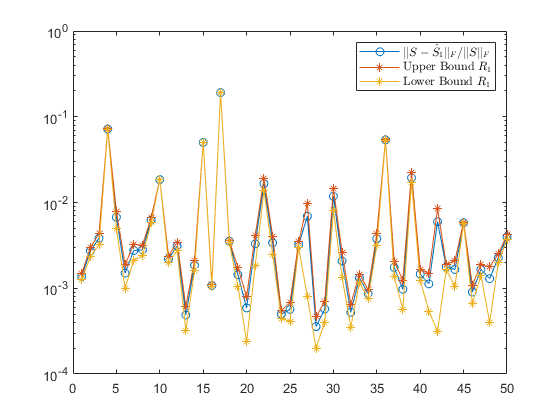
Figure 1: The plots show the effect of an eigenvalues modification when λ1∈σ⁡(S)\lambda_{1}\in\sigma(S) undergoes a relative change of |λ1||\lambda_{1}|. Fifty experiments have been performed with S∈M200​(ℂ)S\in\textnormal{{M}}_{200}(\mathbb{C}). The plots show the use of S^1=(I2​n+X​R1​XT​JT)​S\hat{S}_{1}=(I_{2n}+XR_{1}X^{T}J^{T})S for R1R_{1} in (23), the coarse bound in (26) (left plot), the upper and lower bounds from Theorem 5 (right plot) and the relative change in the eigenvalue |λ1−μ|/|λ1||\lambda_{1}-\mu|/|\lambda_{1}|.

In Figure 1, 50 examples are shown where a randomly selected eigenvalue λ1\lambda_{1} of SS has been changed to μ=λ1​(1+γ​z)\mu=\lambda_{1}(1+\gamma z), where z∈ℂz\in\mathbb{C} is a random complex number with |z|=1|z|=1 and γ=|λ1|\gamma=|\lambda_{1}|. Therefore, |μ−λ1|/|λ1|=|λ1||\mu-\lambda_{1}|/|\lambda_{1}|=|\lambda_{1}|. The plot shows the relative change ‖S−S^1‖F/‖S‖F\|S-\hat{S}_{1}\|_{F}/\|S\|_{F}, the coarse bound in (26), the upper and lower bounds from Theorem 5 and the relative change in the eigenvalue |λ1−μ|/|λ1||\lambda_{1}-\mu|/|\lambda_{1}|. The plots show clearly that the bounds from Theorem 5 are significantly sharper than the bound from (26). If R2R_{2} is used instead of R1R_{1} the plots do not alter essentially.

The most significant difference between using S^1\hat{S}_{1} and S^2\hat{S}_{2} can be seen when an eigenvalue is subject to a small or large relative change compared to its absolute value. This is shown in Figure 2 where the experimental set-up is the same as before but now γ=10−3​|λ1|\gamma=10^{-3}|\lambda_{1}| (left plot) and γ=103​|λ1|\gamma=10^{3}|\lambda_{1}| (right plot) are chosen. Both plots show the relative change ‖S−S^j‖F/‖S‖F\|S-\hat{S}_{j}\|_{F}/\|S\|_{F} for j=1,2j=1,2 and the relative change in the eigenvalue |λ1−μ|/|λ1||\lambda_{1}-\mu|/|\lambda_{1}|. It is seen that for a small change in the eigenvalue λ1\lambda_{1}, the relative change ‖S−S^1‖F/‖S‖F\|S-\hat{S}_{1}\|_{F}/\|S\|_{F} is significantly smaller than ‖S−S^2‖F/‖S‖F\|S-\hat{S}_{2}\|_{F}/\|S\|_{F}. However, when λ1\lambda_{1} undergoes a large change, then there is no big difference in using R1R_{1} or R2R_{2}.

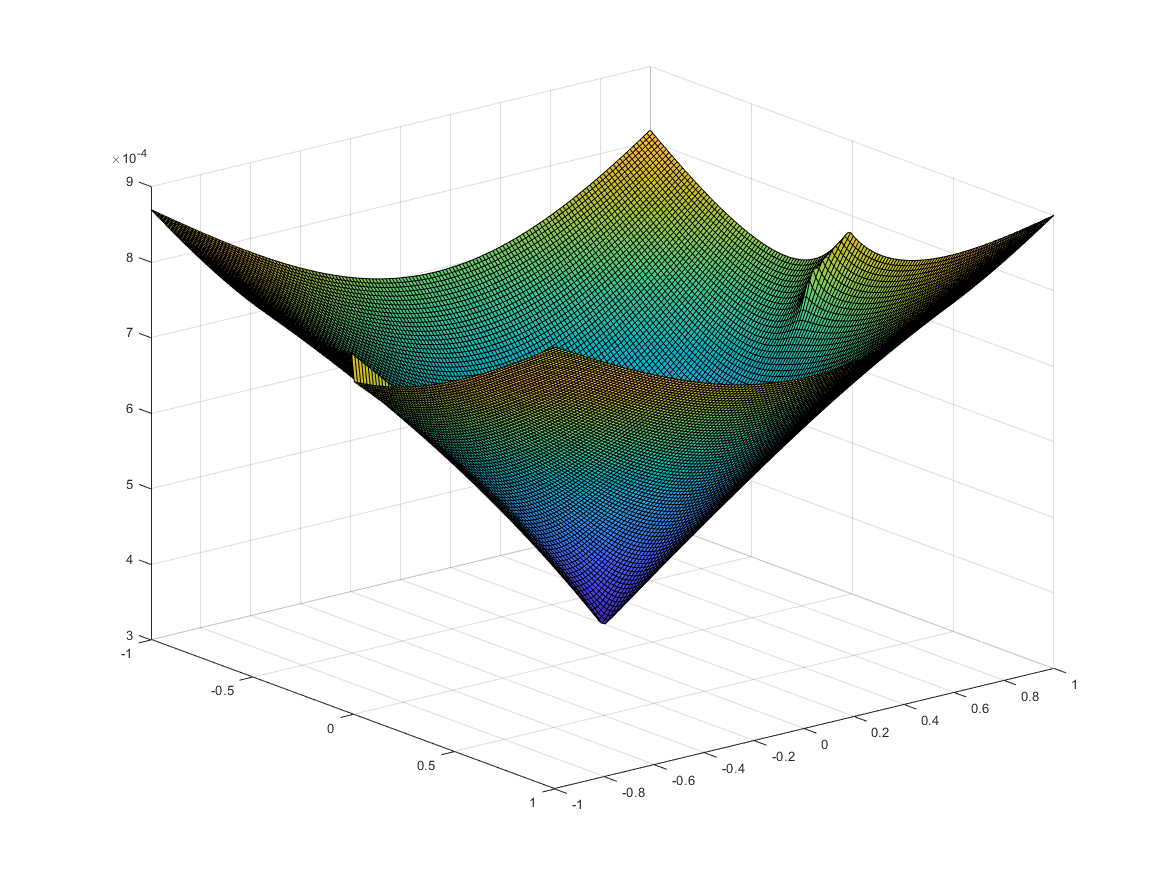
In Figure 3 we show the use of matrices RR different from R1R_{1} and R2R_{2} in (23). To this end, we fix a symplectic matrix S∈M200​(ℂ)S\in\textnormal{{M}}_{200}(\mathbb{C}) and an eigenvalue λ1\lambda_{1} of SS that is to be modified by a relativ change of |λ1||\lambda_{1}|. We consider a mesh grid on [−1,1]×[−1,1][-1,1]\times[-1,1] with 150 discretization points in each direction. Each point (xj,yk)(x_{j},y_{k}) is associated with the complex number cj​k:=xj+ı​ykc_{jk}:=x_{j}+\imath y_{k} from which we made up r11=r22=cj​kr_{11}=r_{22}=\sqrt{c_{jk}}. The values for r12r_{12} and r21r_{21} are found according to (20) and (21) so that we obtain two different matrices R~1=R⁡(η1,r11,r22)\tilde{R}_{1}=R(\eta_{1},r_{11},r_{22}) and R~2=R⁡(η2,r11,r22)\tilde{R}_{2}=R(\eta_{2},r_{11},r_{22}). The matrices S~j=(I2​n+X​R~j​XT​JT)​S\tilde{S}_{j}=(I_{2n}+X\tilde{R}_{j}X^{T}J^{T})S, j=1,2j=1,2, where constructed and in Figure 3 the minimum of ‖S−S~j‖F/‖S‖F\|S-\tilde{S}_{j}\|_{F}/\|S\|_{F} is shown for each point cj​k∈[−1,1]×[−1,1]c_{jk}\in[-1,1]\times[-1,1]. The plot indicates that the minimum numerically found among all values ‖S−S~j‖F/‖S‖F\|S-\tilde{S}_{j}\|_{F}/\|S\|_{F} is attained for cj​k=0c_{jk}=0, i.e. r11=r22=0r_{11}=r_{22}=0. Thus, the minimum is obtained for one of the matrices RR in (23). In most examples that have been considered a plot similar to the one in Figure 3 arose. However, seldom the numerical minimum was detected somewhere near cj​k=0c_{jk}=0.

Refer to caption
Refer to caption
Figure 2: The plots show the effect of an eigenvalues modification when λ1∈σ⁡(S)\lambda_{1}\in\sigma(S) undergoes a relative change of 0.001⋅|λ1|0.001\cdot|\lambda_{1}| (left plot) and 1000⋅|λ1|1000\cdot|\lambda_{1}| (right plot). Fifty experiments have been performed with S∈M200​(ℂ)S\in\textnormal{{M}}_{200}(\mathbb{C}). The plots show the use of S^1\hat{S}_{1} and S^2\hat{S}_{2} and the relative change in the eigenvalue |λ1−μ|/|λ1||\lambda_{1}-\mu|/|\lambda_{1}|.
Refer to caption
Figure 3: The plot shows the minimum of ‖S−S~j‖F/‖S‖F\|S-\tilde{S}_{j}\|_{F}/\|S\|_{F} for j=1,2j=1,2 on the square [−1,1]×[−1,1][-1,1]\times[-1,1] with 150 discretization points in each direction. The minimum on the grid is attained for cj​k=0c_{jk}=0, i.e. r11=r22=0r_{11}=r_{22}=0. For random experiments the plots always look similar to the plot shown above. Notice that the surface has a sharp edge which arises due to the complex square root that has to be computed.

6. Symplectic Matrix Pencils

In this section we analyse the eigenvalue modification problem of Section 1 for symplectic matrix pencils. We call a matrix pencil P⁡(λ)=A−λ​BP(\lambda)=A-\lambda B, A,B∈M2​n​(ℂ)A,B\in\textnormal{{M}}_{2n}(\mathbb{C}) symplectic (see [6, Sec. 2.1.1]) if it holds that

A​J​AT=B​J​BT.AJA^{T}=BJB^{T}. (39)

From (39) it follows that for a symplectic pencil P⁡(λ)=A−λ​BP(\lambda)=A-\lambda B either AA and BB are both regular or singular, cf. [6, Sec. 2]. A scalar ν∈ℂ\nu\in\mathbb{C} is called an eigenvalue of P⁡(λ)P(\lambda) if there exists some nonzero x∈ℂ2​nx\in\mathbb{C}^{2n} with P⁡(ν)​x=0P(\nu)x=0, i.e. A​x=ν​B​xAx=\nu Bx [2, Sec. 2]. Eigenvalues of symplectic pencils also arise in pairs (ν,ν−1)(\nu,\nu^{-1}) [6]. In particular, if AA and BB are singular, it is also possible to have ν=0\nu=0 as an eigenvalue of P⁡(λ)P(\lambda) which implies that λ−1=∞\lambda^{-1}=\infty is also an eigenvalue of P⁡(λ)P(\lambda) (see, e.g., [5] for more information on the finite and infinite eigenstructure of matrix pencils). In the following, we focus on symplectic pencils P⁡(λ)=A−λ​BP(\lambda)=A-\lambda B where both AA and BB are regular. Thus, P⁡(λ)P(\lambda) has neither the eigenvalue zero nor the eigenvalue infinity.

In general, for an arbitrary matrix pencil P⁡(λ)=A−λ​BP(\lambda)=A-\lambda B, A,B∈Mn​(ℂ)A,B\in\textnormal{{M}}_{n}(\mathbb{C}), where BB is nonsingular, we can easily derive an adapted version of Rado’s theorem.

Theorem 10.

Let P⁡(λ)=A−λ​BP(\lambda)=A-\lambda B, A,B∈Mn​(ℂ)A,B\in\textnormal{{M}}_{n}(\mathbb{C}) and BB nonsingular, be a matrix pencil with eigenvalues λ1,…,λn∈ℂ\lambda_{1},\ldots,\lambda_{n}\in\mathbb{C}. Let x1,…,xk∈ℂnx_{1},\ldots,x_{k}\in\mathbb{C}^{n} be eigenvectors for λ1,…,λk\lambda_{1},\ldots,\lambda_{k} such that rank​(X)=k\textnormal{rank}(X)=k for X=[x1x2⋯xk]∈Mn×k(ℂ)X=[\,x_{1}\;x_{2}\;\cdots\;x_{k}\,]\in\textnormal{{M}}_{n\times k}(\mathbb{C}). Furthermore, let C∈Mn×k​(ℂ)C\in\textnormal{{M}}_{n\times k}(\mathbb{C}) be arbitrary. Then the matrix pencil

P~​(λ)=(A+B​X​CT)−λ​B\tilde{P}(\lambda)=(A+BXC^{T})-\lambda B

has the eigenvalues μ1,…,μk,λk+1,…,λn\mu_{1},\ldots,\mu_{k},\lambda_{k+1},\ldots,\lambda_{n}, where μ1,…,μk\mu_{1},\ldots,\mu_{k} are the eigenvalues of the matrix Λ+CT​X\Lambda+C^{T}X with Λ=diag​(λ1,…,λk)\Lambda=\textnormal{diag}(\lambda_{1},\ldots,\lambda_{k}).

Proof.

As B−1​P​(λ)=B−1​A−λ​InB^{-1}P(\lambda)=B^{-1}A-\lambda I_{n}, the eigenvalues of P⁡(λ)P(\lambda) coincide with those of the matrix M:=B−1​A∈M2​n​(ℂ)M:=B^{-1}A\in\textnormal{{M}}_{2n}(\mathbb{C}). In particular, P⁡(λ)P(\lambda) does not have λ=∞\lambda=\infty as an eigenvalue. Assume that A​X=B​X​ΛAX=BX\Lambda with Λ=diag​(λ1,…,λk)\Lambda=\textnormal{diag}(\lambda_{1},\ldots,\lambda_{k}) we obtain B−1​A​X=X​ΛB^{-1}AX=X\Lambda and Theorem 2 implies that M^:=B−1​A+X​CT\hat{M}:=B^{-1}A+XC^{T} has the eigenvalues μ1,…,μk,λk+1,…,λn\mu_{1},\ldots,\mu_{k},\lambda_{k+1},\ldots,\lambda_{n}, where μ1,…,μk\mu_{1},\ldots,\mu_{k} are the eigenvalues of the matrix Λ+CT​X\Lambda+C^{T}X. As M^\hat{M} and the matrix pencil P^​(λ)=(A+B​X​CT)−λ​B\hat{P}(\lambda)=(A+BXC^{T})-\lambda B have the same eigenvalues, the statement follows. ∎

Now let P⁡(λ)=A−λ​BP(\lambda)=A-\lambda B be a symplectic matrix pencil according to (39) with nonsingular A,BA,B and eigenvalues λ1,λ1−1,…,λn,λn−1\lambda_{1},\lambda_{1}^{-1},\ldots,\lambda_{n},\lambda_{n}^{-1}. We set

P^​(λ):=(A+B​X​CT)−λ​B\hat{P}(\lambda):=(A+BXC^{T})-\lambda B

and intend to determine C∈M2​n×2​(ℂ)C\in\textnormal{{M}}_{2n\times 2}(\mathbb{C}) such that P^​(λ)\hat{P}(\lambda) is again symplectic and has the eigenvalues μ,μ−1,λ2,λ2−1,…,λn,λn−1\mu,\mu^{-1},\lambda_{2},\lambda_{2}^{-1},\ldots,\lambda_{n},\lambda_{n}^{-1} for a given value μ∈ℂ∖{0}\mu\in\mathbb{C}\setminus\{0\}. A direct calculation reveals that (39) is equivalent to B−1​AB^{-1}A being a symplectic matrix, i.e. JT​(B−1​A)T​J=(B−1​A)−1J^{T}(B^{-1}A)^{T}J=(B^{-1}A)^{-1}. Thus, Theorem 3 can be applied to the matrix S:=B−1​AS:=B^{-1}A that has the same eigenvalues as P⁡(λ)P(\lambda). Now suppose

A​X=B​X​[λ1λ1−1],X=[x1x2]∈M2​n×2​(ℂ),AX=BX\begin{bmatrix}\lambda_{1}&\\ &\lambda_{1}^{-1}\end{bmatrix},\qquad X=\begin{bmatrix}x_{1}&x_{2}\end{bmatrix}\in\textnormal{{M}}_{2n\times 2}(\mathbb{C}),

i.e. x1,x2∈ℂ2​nx_{1},x_{2}\in\mathbb{C}^{2n} are generalized eigenvectors for λ1\lambda_{1} and λ1−1\lambda_{1}^{-1}, respectively. Furthermore, assume x1T​J​x2≠0x_{1}^{T}Jx_{2}\neq 0. Then

S^:=B−1​A+X​R​XT​JT​B−1​A\hat{S}:=B^{-1}A+XRX^{T}J^{T}B^{-1}A

is symplectic with eigenvalues μ,μ−1,λ2,λ2−1,…,λn,λn−1\mu,\mu^{-1},\lambda_{2},\lambda_{2}^{-1},\ldots,\lambda_{n},\lambda_{n}^{-1} provided that RR is chosen according to the conditions in Theorem 3 for μ\mu. Then, the matrix pencil P^​(λ):=B⁡(S^−λ​I2​n)\hat{P}(\lambda):=B(\hat{S}-\lambda I_{2n}), i.e.

P^​(λ)=(A+B​X​R​XT​JT​B−1​A)−λ​B,\hat{P}(\lambda)=\big(A+BXRX^{T}J^{T}B^{-1}A\big)-\lambda B, (40)

has the same eigenvalues as S^\hat{S} [5, Sec. 3.1]. In fact, P^​(λ)\hat{P}(\lambda) is again a symplectic pencil. To show this, we have to check that

(A+B​X​R​XT​JT​B−1​A)​J​(A+B​X​R​XT​JT​B−1​A)T=B​J​BT\big(A+BXRX^{T}J^{T}B^{-1}A\big)J\big(A+BXRX^{T}J^{T}B^{-1}A\big)^{T}=BJB^{T}

holds. To this end, it only remains to prove that

A​J​(B​X​R​XT​JT​B−1​A)T+(B​X​R​XT​JT​B−1​A)​J​AT\displaystyle AJ\big(BXRX^{T}J^{T}B^{-1}A\big)^{T}+\big(BXRX^{T}J^{T}B^{-1}A\big)JA^{T} (41)
+(B​X​R​XT​JT​B−1​A)​J​(B​X​R​XT​JT​B−1​A)T=0\displaystyle+\big(BXRX^{T}J^{T}B^{-1}A\big)J\big(BXRX^{T}J^{T}B^{-1}A\big)^{T}=0

since A​J​AT=B​J​BTAJA^{T}=BJB^{T} holds by assumption. Using this relation, (41) simplifies to

−B​X​RT​XT​BT+B​X​R​XT​BT+B​X​R​J2​RT​XT​BT=0-BXR^{T}X^{T}B^{T}+BXRX^{T}B^{T}+BXRJ_{2}R^{T}X^{T}B^{T}=0

which can be rewritten as B​X​(R−RT+R​J2​RT)​XT​BT=0BX\big(R-R^{T}+RJ_{2}R^{T}\big)X^{T}B^{T}=0. As in Section 2 this relation holds if and only if R−RT+R​J2​RT=0R-R^{T}+RJ_{2}R^{T}=0. As for any R∈M2​(ℂ)R\in\textnormal{{M}}_{2}(\mathbb{C}) we have R​J2​RT=RT​J2​RRJ_{2}R^{T}=R^{T}J_{2}R, it follows that the condition R−RT+R​J2​RT=0R-R^{T}+RJ_{2}R^{T}=0 is equivalent to (6). Therefore, since RR was constructed according to (13) so that R−RT+RT​J2​R=0R-R^{T}+R^{T}J_{2}R=0 holds, this finally shows that (41) is true, so P^​(λ)\hat{P}(\lambda) is symplectic. As already mentioned above, P^​(λ)\hat{P}(\lambda) and S^\hat{S} have the same eigenvalues, so the eigenvalues of P^​(λ)\hat{P}(\lambda) are μ,μ−1,λ2,λ2−1,…,λn,λn−1\mu,\mu^{-1},\lambda_{2},\lambda_{2}^{-1},\ldots,\lambda_{n},\lambda_{n}^{-1}.

Notice that P^​(λ)\hat{P}(\lambda) in (40) can be rewritten in various ways, e.g.

P^​(λ)\displaystyle\hat{P}(\lambda) =(A+B​X​R​XT​BT​A−T​JT)−λ​B\displaystyle=\big(A+BXRX^{T}B^{T}A^{-T}J^{T}\big)-\lambda B (42)
=(A+B​X​R​XT​BT​JT​A)−λ​B\displaystyle=\big(A+BXRX^{T}B^{T}J^{T}A\big)-\lambda B (43)

using the relation JT​B−1​A=BT​A−T​JTJ^{T}B^{-1}A=B^{T}A^{-T}J^{T} that follows from B−1​AB^{-1}A being symplectic in (42) and A−T=JT​A​JA^{-T}=J^{T}AJ in (43). Using XT​BT=Λ−1​XT​ATX^{T}B^{T}=\Lambda^{-1}X^{T}A^{T} and exchanging XT​BTX^{T}B^{T} with Λ−1​XT​AT\Lambda^{-1}X^{T}A^{T} in (42) yields

P^​(λ)\displaystyle\hat{P}(\lambda) =(A+B​X​R​Λ−1​XT​AT​A−T​JT)−λ​B\displaystyle=(A+BXR\Lambda^{-1}X^{T}A^{T}A^{-T}J^{T})-\lambda B
=(A+B​X​R​[λ1−1λ1]​XT​JT)−λ​B.\displaystyle=\left(A+BXR\begin{bmatrix}\lambda_{1}^{-1}&\\ &\lambda_{1}\end{bmatrix}X^{T}J^{T}\right)-\lambda B. (44)

which is an expression for P^​(λ)\hat{P}(\lambda) similar to (14). We conclude our finding in the following theorem.

Theorem 11.

Let P⁡(λ)=A−λ​BP(\lambda)=A-\lambda B, A,B∈M2​n​(ℂ)A,B\in\textnormal{{M}}_{2n}(\mathbb{C}) nonsingular, be a symplectic pencil with eigenvalues λ1,λ1−1,λ2,λ2−1,\lambda_{1},\lambda_{1}^{-1},\lambda_{2},\lambda_{2}^{-1}, …,λn,λn−1∈ℂ\ldots,\lambda_{n},\lambda_{n}^{-1}\in\mathbb{C} and let μ∈ℂ∖{0}\mu\in\mathbb{C}\setminus\{0\} be given. Let x1,x2∈ℂ2​nx_{1},x_{2}\in\mathbb{C}^{2n} be eigenvectors for λ1\lambda_{1} and λ1−1\lambda_{1}^{-1}, respectively, normalized such that XT​J2​n​X=J2X^{T}J_{2n}X=J_{2} for X=[x1​x2]∈M2​n​(ℂ)X=[\;x_{1}\;x_{2}\;]\in\textnormal{{M}}_{2n}(\mathbb{C}) and set d:=(μ+μ−1)−(λ1+λ1−1)d:=(\mu+\mu^{-1})-(\lambda_{1}+\lambda_{1}^{-1}). Then the matrix pencil

P^​(λ):=(A+B​X​R​[λ1−1λ1]​XT​J)−λ​B\hat{P}(\lambda):=\left(A+BXR\begin{bmatrix}\lambda_{1}^{-1}&\\ &\lambda_{1}\end{bmatrix}X^{T}J\right)-\lambda B (45)

is again symplectic and has the eigenvalues μ,μ−1,λ2,λ2−1,…,λn,λn−1\mu,\mu^{-1},\lambda_{2},\lambda_{2}^{-1},\ldots,\lambda_{n},\lambda_{n}^{-1} provided that R=[ri​j]i​j∈M2​(ℂ)R=[r_{ij}]_{ij}\in\textnormal{{M}}_{2}(\mathbb{C}) is chosen such that (12) and (13) hold.

Regarding P^​(λ)\hat{P}(\lambda) in (40), let P^​(λ)=A^−λ​B^\hat{P}(\lambda)=\hat{A}-\lambda\hat{B} with A^=A+B​X​R​XT​JT​B−1​A\hat{A}=A+BXRX^{T}J^{T}B^{-1}A and B^=B\hat{B}=B. Then certainly ‖B^−B‖/‖B‖=0\|\hat{B}-B\|/\|B\|=0 while

‖A^−A‖‖A‖≤κ⁡(B)​‖R‖​‖X‖2,\frac{\|\hat{A}-A\|}{\|A\|}\leq\kappa(B)\|R\|\|X\|^{2},

where κ⁡(B)=‖B‖​‖B−1‖\kappa(B)=\|B\|\|B^{-1}\| is the condition number of the matrix BB. Thus, using Theorem 5 we may immediately bound ‖A^−A‖/‖A‖\|\hat{A}-A\|/\|A\|. Furthermore, from the form of P^​(λ)\hat{P}(\lambda) in (45), statements similar to those in Section 4.2 can directly be derived.

7. Summary

In this work we showed how to modify a pair of eigenvalues λ,1/λ\lambda,1/\lambda of a symplectic matrix SS to desired target values μ,1/μ\mu,1/\mu for a symplecitc matrix S^\hat{S} in a structure-preserving way. Universal bounds on the relative distance between SS and S^\hat{S} with modified spectrum were given. The eigenvalues Segre characteristics of SS were related to those of SS and some statements on eigenvalue condition numbers have been derived. The main results have been extended to matrix pencils.

8. Acknowledgement

The author is grateful to Thomas Richter as this work was in parts developed during the authors employment in Thomas Richter’s group at the Otto-von-Guericke-Universität Magdeburg.

References

  • [1] A. T. Alexandridis, H. E. Psillakis. The inverse optimal LQR problem and its relation to passivity and eigenvalue assignment. International Journal of Tomography & Statistics, Vol. 5, 2007.
  • [2] T. Betcke, N. J. Higham, V. Mehrmann, C. Schröder, F. Tisseur. NLEVP: A Collection of Nonlinear Eigenvalue Problems. ACM Transactions on Mathematical Software, Vol. 39(2), 2013.
  • [3] R. Bru, R. Canto, R. L. Soto and A. M. Urbano A Brauer’s theorem and related Results. Cent. Eur. J. Math. 10(1), 2012.
  • [4] D. F. Delchamps. State Space and Input-Output Linear Systems. Springer Verlag, New York, USA, 1988.
  • [5] F. De Terán, F. M. Dopico, D. S. Mackey. Spectral equivalence of matrix polynomials and the Index Sum Theorem. Linear Algebra Appl., Vol. 459, 2014.
  • [6] H. Fassbender. Symplectic Methods for the Symplectic Eigenproblem. Kluwer Academic Publishers, New York, USA, 2002.
  • [7] R. A. Horn, C. R. Johnson. Matrix Analysis (Second Edition). Cambridge University Press, New York, USA, 2013.
  • [8] D. P. Jagger. MATLAB Toolbox for Classical Matrix Groups. Masters thesis, University of Manchester, 2003. MIMS EPrint 2007.99.
  • [9] C. R. Johnson, E. A. Schreiner. The Relationship between A​BAB and B​ABA. The American Mathematical Monthly, Vol. 103(7), 1996.
  • [10] A. J.Laub, K. Meyer. Canonical Forms for Symplectic and Hamiltonian Matrices. Celestial Mechanics, Vol. 9, 1974.
  • [11] D. G. Luenberger. Optimization by Vector Space Methods. John Wiley & Sons, Inc., New York, USA, 1969.
  • [12] T. Lyche. Numerical Linear Algebra and Matrix Factorizations. Springer Nature, Cham, Switzerland, 2020.
  • [13] H. Perfect. Methods of constructing certain stochastic matrices. II Duke Math. J. 22(2), 1955.
  • [14] Y. Saad. Numerical Methods for Large Eigenvalue Problems (Revised Edition). Society for Industrial and Applied Mathematics, Philadelphia, USA, 2011.
  • [15] H. Shapiro. Linear Algebra and Matrices. Topics for a Second Course. American Mathematical Society, Providence, USA, 2015.
  • [16] R. L. Soto and O. Rojo. Applications of a Brauer theorem in the nonnegative inverse eigenvalue problem. Linear Algebra Appl. 416(2-3), 2006.
  • [17] O. Taussky, H. Zassenhaus. On the similarity transformation between a matirx and its transpose. Pacific J. Math. 9(3), 1959.