Passivity-based power sharing and voltage regulation in DC microgrids with unactuated buses

Albertus Johannes Malan Pol Jané-Soniera Felix Strehle Sören Hohmann Thanks: This work was supported in part by Germany’s Federal Ministry for Economic Affairs and Climate Action (BMWK) through the RegEnZell project (reference number 0350062C). (Corresponding author: A. J. Malan.) Thanks: A. J. Malan, P. Jané-Soniera, F. Strehle, and S. Hohmann are with the Institute of Control Systems (IRS), Karlsruhe Institute of Technology (KIT), 76131, Karlsruhe, Germany. Emails: albertus.malan@kit.edu, pol.soneira@kit.edu, felix.strehle@kit.edu, soeren.hohmann@kit.edu.

Abstract

In this paper, we propose a novel four-stage distributed controller for a DC microgrid that achieves power sharing and average voltage regulation for the voltages at actuated and unactuated buses. The controller is presented for a DC microgrid comprising multiple distributed generating units (DGUs) with time-varying actuation states; dynamic RLC lines; nonlinear constant impedance, current and power (ZIP) loads and a time-varying network topology. The controller comprising a nonlinear gain, PI controllers, and two dynamic distributed averaging stages is designed for asymptotic stability. This constitutes first deriving passivity properties for the DC microgrid, along with each of the controller subsystems. Thereafter, design parameters are found through a passivity-based optimisation using the worst-case subsystem properties. The resulting closed-loop is robust against DGU actuation changes, network topology changes, and microgrid parameter changes. The stability and robustness of the proposed control is verified via simulations.

Index Terms:

DC microgrids, distributed control, passivity, power sharing, voltage regulation.

I Introduction

The advent of localised power generation and storage increasingly challenges the prevailing centralised power-generation structures. Originally proposed in [1], the microgrids paradigm envisions networks that can operate autonomously through advanced control while meeting consumer requirements. Although current electrical grids predominantly use AC, high and low voltage DC networks have been made technically feasible due to the continual improvements of power electronics. Indeed, DC microgrids exhibit significant advantages over their AC counterparts, demonstrating a higher efficiency and power quality while simultaneously being simpler to regulate [2, 3].

In microgrids, power generation and storage units are typically grouped into DGU which connect to the microgrid through a single DC-DC converter for higher efficiency [2]. This changes the traditionally centralised regulation problem in power grids into a problem of coordinating the DGU connected throughout the microgrid. This coordination is generally realised as average or global voltage regulation in combination with load sharing between the DGU (see e.g. [4, 5, 6]).

Literature Review

A vast number of approaches have been proposed for the voltage regulation and load sharing of DC microgrids, as detailed in the overview papers [7, 3, 8] along with the sources therein. These approaches are broadly categorised as either centralised, decentralised or distributed in nature [7, 3, 8]. While centralised controllers can optimally coordinate the DGU, they offer reduced scalability and flexibility and have a single point of failure [8]. On the other hand, decentralised controllers either only attempt to achieve voltage stability [9, 10, 11] or achieve load sharing at the cost of voltage regulation quality (e.g. the droop-based approaches in [3]).

In response to these limitations, numerous controllers for voltage regulation and load sharing which operate in a distributed manner have been proposed [4, 5, 12, 13, 14, 15, 16, 17, 6, 18, 19, 20]. In [4], distributed averaging is employed to find a global voltage estimate with which voltage regulation is achieved, but the microgrid dynamics are neglected in the stability analysis. Distributed averaging with dynamic microgrid models is used in [5, 12], although [5] requires LMIs to be solved before buses are allowed to connect whereas [12] only considers constant current loads. Similarly, a sliding-mode controller is proposed in [13] for a dynamic microgrid with constant current loads. On the other hand, [14] proposes a cyberattack-resilient controller for a microgrid with constant conductance loads and resistive lines. A consensus-based distributed controller with event-triggered communication is presented in [15]. Consensus-based controllers are also utilised in [16, 17, 6], where [6] uses a consensus-based integral layer on top of a droop-based controller. Finally, while many contributions strive to achieve proportional current sharing [4, 5, 12, 13, 14, 15, 16, 17, 6, 20], nonlinear controllers that achieve proportional power sharing have also been proposed in [18, 19].

While the literature listed above differ greatly in their approaches, we note a commonality in their omission of buses without actuation. This omission is typically motivated either by considering a microgrid comprising only actuated DGU buses [4, 5, 16, 17], or by eliminating the unactuated buses with the Kron-reduction [12, 13, 14, 15, 6, 18, 19, 20]. However, considering a network comprising only actuated buses severely limits the flexibility of a microgrid, since each bus must be able to supply or consume enough power at all times. On the other hand, the Kron-reduction requires loads to be described as positive conductances (see e.g. [21]). While research into Kron-reduced networks with negative loads is ongoing (see e.g. [22]), the general inclusion of negative loads, e.g. non-controllable power sources, in Kron-reducible networks remains out of reach at present. Furthermore, consider the case where a DGU can no longer supply or consume the required amount of power, e.g. a fully charged or discharged battery storage. Such a DGU then loses the ability to regulate itself and fully support the grid. In the approaches considered above [4, 5, 12, 13, 14, 15, 16, 17, 6, 18, 19, 20], such a DGU is forced to disconnect from the microgrid and its local measurements are discarded. For DGU with intermittent power sources, this could result in significant swings in the number of controlled and observed buses in the microgrid.

Main Contribution

In this paper, we consider a DC microgrid as a physically interconnected multi-agent system. Extending our work in [23]¹¹ 1 The controller proposed in [23] is extended by weighing the error with a nonlinear function. Moreover, in addition to applying the controller to a DC microgrid context, we here propose a new dissipativity-based analysis that investigates the closed loop stability analytically as opposed to the numerical results in [23]., we propose a four-stage controller that achieves voltage regulation and power sharing in a DC microgrid with actuated and unactuated buses in a distributed manner. The four-stage controller comprises a nonlinear weighting function, two DDA (DDA) stages and a PI (PI) controller. The asymptotic stability of the closed loop comprising the DC microgrid and the four-stage controller interconnected in feedback is proven by means of passivity theory. In detail, the contributions comprise:

1.

A four-stage distributed controller for DC microgrids which achieves consensus on the weighted average voltage error of actuated and unactuated buses and assures coordination through power sharing at the actuated buses.
2.

A nonlinear weighting function that penalises voltage errors outside a given tolerance band more strongly than those within.
3.

Passivity classifications for each of the constitutive microgrid subsystems (DGU, loads, and lines) and for each of the controller stages (weighting function, DDA, and PI).
4.

A method for calculating the IFOFP (IFOFP) indices of the nonlinear power-controlled DGU through optimisation.
5.

An IFOFP formulation for the DC microgrid with a supply rate that is independent of the network topology, the number of buses and their states of actuation.
6.

A passivity-based stability analysis for the equilibrium of the DC microgrid connected in feedback with the four-stage controller.

In addition to the contributions listed above, we also contribute a theoretical result comprising a formalisation of the obstacle presented by cascaded IFP (IFP) and OFP (OFP) systems in the analysis of dissipative systems. This theoretical contribution informs and motivates parameter choices for the four-stage controller in Contribution 1.

We highlight that the proposed controller can achieve exact voltage regulation and power sharing with the stability verified with the eigenvalues of the linearised system. Moreover, by employing leaky PI controllers, we demonstrate a passivity-based stability analysis that is independent of and robust against changes in the communication topology, changes in the electrical topology, load changes, changes in the actuation status of DGU, uncertainties in component parameters, and buses connecting or disconnecting.

Paper Organisation

The introduction concludes with some notation and preliminaries on graph theory. In Section II, we recall and introduce results relating to dissipativity theory. Next, in Section III, the problem is modelled and objectives for the steady state are formalised. In Section IV, a four-stage control structure is introduced that fulfils objectives from Section III. Thereafter, the passivity properties of the constituent subsystems are investigated in Section V and the controller is designed for asymptotic stability of the closed loop in Section VI. Finally, in Section VII, a simulation is used to verify the asymptotic stability and robustness of the closed loop. Concluding remarks are provided in Section VIII.

Notation and Preliminaries

Define as a vector $\bm{a}=(a_{k})$ and a matrix $\bm{A}=(a_{kl})$ . $\bm{\mathds{1}}_{k}$ is a $k$ -dimensional vector of ones and $\bm{I}_{k}$ is the identity matrix of dimension $k$ . $\Diag[\cdot]$ creates a (block-)diagonal matrix from the supplied vectors (or matrices). The upper and lower limits of a value $a$ are given by $\overline{a}$ and $\underline{a}$ . For a variable $x$ , we denote its unknown steady state as $\hat{x}$ , its error state as $\tilde{x}\coloneqq x-\hat{x}$ , and a desired setpoint as ${x}^{*}$ . Whenever clear from context, we omit the time dependence of variables.

We denote by $\mathcal{G}=(\mathcal{N},\mathcal{E})$ a finite, weighted, undirected graph with vertices $\mathcal{N}$ and edges $\mathcal{E}\subseteq\mathcal{N}\times\mathcal{N}$ . Let $|\mathcal{N}|$ be the cardinality of the set $\mathcal{N}$ . Let $\bm{\mathcal{L}}$ be the Laplacian matrix of $\mathcal{G}$ . By arbitrarily assigning directions to each edge in $\mathcal{E}$ , the incidence matrix $\bm{E}\in\mathbb{R}^{|\mathcal{N}|\times|\mathcal{E}|}$ of $\mathcal{G}$ is defined by

e_{kl}=\left\{\begin{array}[]{@{}rl}+1&\text{if vertex $k$ is the sink of edge $l$},\\ -1&\text{if vertex $k$ is the source of edge $l$},\\ 0&\text{otherwise}.\end{array}\right.

(1)

II Dissipativity Preliminaries

We here recall and introduce preliminaries of dissipativity theory for nonlinear systems. In Section II-A we provide definitions relating to dissipativity and passivity theory. Thereafter in Section II-B, we investigate the passivity properties of static functions. Finally, in Section II-C, we recall a result on the interconnection of dissipative systems with quadratic supply rates and formalise a new result on the limitations of such an interconnection.

II-A Dissipative Systems

Consider a nonlinear system

\left\{\begin{aligned} \dot{\bm{x}}&=\bm{f}(\bm{x},\bm{u}),\\ \bm{y}&=\bm{h}(\bm{x}),\end{aligned}\right.

(2)

where $\bm{x}\in\mathbb{R}^{n}$ , $\bm{u}\in\mathbb{R}^{m}$ , $\bm{y}\in\mathbb{R}^{m}$ and where $\bm{f}\colon\mathbb{R}^{n}\times\mathbb{R}^{m}\rightarrow\mathbb{R}^{n}$ and $\bm{h}\colon\mathbb{R}^{n}\times\mathbb{R}^{m}\rightarrow\mathbb{R}^{m}$ are class $C^{1}$ functions.

Definition 1 (Dissipative system, c.f. [24, 25, 26]).

A system (2) with a class $C^{1}$ storage function $\cramped{S\colon\mathbb{R}^{n}\times\mathbb{R}^{m}\rightarrow\mathbb{R}_{+}}$ is dissipative w.r.t. a supply rate $w(\bm{u},\bm{y})$ if $\dot{S}\leq w(\bm{u},\bm{y})$ .

Definition 2 (Quadratic supply rates, c.f. [24, 25, 26]).

A system (2) that is dissipative w.r.t. $w(\bm{u},\bm{y})$ is

•

passive if $w=\bm{u}^{T}\bm{y}$ ,
•

IFP (IFP) if $w=\bm{u}^{T}\bm{y}-\nu\bm{u}^{T}\bm{u}$ ,
•

OFP (OFP) if $w=\bm{u}^{T}\bm{y}-\rho\bm{y}^{T}\bm{y}$ ,
•

IFOFP (IFOFP) if $w=\cramped{(1+\nu\rho)}\bm{u}^{T}\bm{y}-\nu\bm{u}^{T}\bm{u}-\rho\bm{y}^{T}\bm{y}$ ,
•

has an $L_{2}$ -gain of $\gamma_{L_{2}}$ if $w=\gamma_{L_{2}}^{2}\bm{u}^{T}\bm{u}-\bm{y}^{T}\bm{y}$ ,

where $\gamma_{L_{2}}>0$ and $\nu,\rho\in\mathbb{R}$ .

Definition 3 ( ZSO (ZSO) [24, p. 46]).

A system (2) is ZSO if $\bm{u}\equiv\bm{0}$ and $\bm{y}\equiv\bm{0}$ implies $\bm{x}\equiv\bm{0}$ .

For cases where the desired equilibrium of a system is not at the origin but at some constant value, the shifted passivity [24, p. 96] or EIP (EIP) [27] of a system must be investigated. Naturally, this requires that an equilibrium exists, i.e. there is a unique input $\hat{\bm{u}}\in\mathbb{R}^{m}$ for every equilibrium $\hat{\bm{x}}\in\hat{\mathcal{X}}\subset\mathbb{R}^{n}$ such that (2) produces $\bm{f}(\hat{\bm{x}},\hat{\bm{u}})=0$ and $\hat{\bm{y}}=\bm{h}(\hat{\bm{x}},\hat{\bm{u}})$ [28, p. 24].

Definition 4 (EIP [28, p. 24]).

A system (2) is EIP if there exists a class $C^{1}$ storage function $S(\bm{x},\hat{\bm{x}},\bm{u})$ , $\cramped{S\colon\mathbb{R}^{n}\times\hat{\mathcal{X}}\times\mathbb{R}^{m}\rightarrow\mathbb{R}_{+}}$ , with $S(\hat{\bm{x}},\hat{\bm{x}},\hat{\bm{u}})=0$ , that is dissipative w.r.t. $w(\bm{u}-\hat{\bm{u}},\bm{y}-\hat{\bm{y}})$ for any equilibrium $(\hat{\bm{u}},\hat{\bm{y}})$ .

II-B Passive Static Functions

Recall that a sector-bounded static nonlinear function is dissipative to a supply rate defined by the sector bound [26, Def. 6.2]. We now consider the arbitrarily shifted single-input single-output function

\left\{\begin{aligned} y&=h(u),\quad u,\hat{u}\in\mathcal{U},\quad y,\hat{y}\in\mathcal{Y},\quad h:\mathcal{U}\rightarrow\mathcal{Y},\\ \tilde{y}&=\tilde{h}(\tilde{u})\coloneqq h(u)-h(\hat{u})=y-\hat{y},\quad\tilde{u}\coloneqq u-\hat{u}\end{aligned}\right.

(3)

and show how its dissipativity properties may be derived.

Proposition 5 (EIP static functions).

A static function (3) of class $C^{0}$ is IFOFP $(\underline{c},1/\overline{c})$ w.r.t. the arbitrarily shifted input-output pair $(\tilde{u},\tilde{y})$ if

\underline{c}\leq\dfrac{\text{d}h(u)}{\text{d}u}\leq\overline{c},\quad\forall u\in\mathcal{U}.

(4)

and $0<\overline{c}<\infty$ .

Proof.

Consider for (3) the slope between an arbitrary shift $(\hat{u},\hat{y})\in\mathcal{U}\times\mathcal{Y}$ and a point $(u,y)$ , for which the upper and lower bounds are given by

\underline{c}\leq\frac{y-\hat{y}}{u-\hat{u}}\leq\overline{c},\quad\forall(u,y),(\hat{u},\hat{y})\in\mathcal{U}\times\mathcal{Y}.

(5)

Changing to the shifted variables $\tilde{u}$ and $\tilde{y}$ as in (5) and multiplying through by $\tilde{u}^{2}$ yields

	$\displaystyle\underline{c}\tilde{u}^{2}\leq\tilde{u}\tilde{y}\leq\overline{c}\tilde{u}^{2}$	$\displaystyle\iff(\tilde{y}-\underline{c}\tilde{u})(\tilde{y}-\overline{c}\tilde{u})\leq 0$		(6)
		$\displaystyle\iff(\tilde{y}-\underline{c}\tilde{u})(\frac{1}{\overline{c}}\tilde{y}-\tilde{u})\leq 0,$		(6)

for $\overline{c}>0$ , which describes an IFOFP function (see [26, p. 231]). Finally, through the mean value theorem, the bounds in (5) may be found from (4). ∎

We note that the restrictions on $\overline{c}$ in Prop. 5 are needed from a computational point of view $(\overline{c}<\infty)$ and to ensure that the passivity indices correspond to the correct sector²² 2 Consider e.g. the sector Prop. 5 would yield if $\underline{c}\leq\overline{c}<0$ . $(\overline{c}>0)$ . However, this limits the passivity properties attainable through Prop. 5 to $\rho=1/\overline{c}>0$ .

Remark 1 (Symmetrical sectors).

Placing the additional restriction $\underline{c}=-\overline{c}$ in (4) results in the Lipschitz continuity of $h(u)$ . Moreover, this implies that the arbitrarily shifted function $\tilde{h}(\tilde{u})$ has a finite $L_{2}$ -gain of $\overline{c}$ [29].

II-C Interconnected Quadratic Dissipative Systems

Building upon the results on the interconnection of dissipative systems in [28, 30], we now provide a method for finding dissipativity properties for a subset of the interconnected subsystems such that interconnected stability is guaranteed. Specifically, we look for the dissipative supply rates that restrict the subset of subsystems as little as possible. For a set $\mathcal{S}$ of subsystems, define $\bm{u}=[\bm{u}_{1}^{T},\dots,\bm{u}_{|\mathcal{S}|}^{T}]^{T}$ and $\bm{y}=[\bm{y}_{1}^{T},\dots,\bm{y}_{|\mathcal{S}|}^{T}]^{T}$ .

Theorem 6 (Minimally restrictive stabilising indices).

Consider $|\mathcal{S}|$ subsystems of the form (2) which are dissipative w.r.t. the supply rates $w_{i}=2\sigma_{i}\bm{u}_{i}^{T}\bm{y}_{i}-\nu_{i}\bm{u}_{i}^{T}\bm{u}_{i}-\rho_{i}\bm{y}_{i}^{T}\bm{y}_{i}$ and are linearly interconnected according to $\bm{u}=\bm{H}\bm{y}$ . The stability of the interconnected system is guaranteed if there exists a $\bm{D}$ and $\nu_{j},\rho_{j}\in\mathbb{R}$ with $j\in\mathcal{J}$ such that

\begin{array}[]{cl}\!\displaystyle\underset{\begin{array}[]{c}\\[-15.49997pt] \scriptstyle\bm{D},\,\nu_{j},\,\rho_{j},\\[-3.5pt] \scriptstyle j\in\mathcal{J}\end{array}}{\min}&\!\displaystyle\sum_{j\in\mathcal{J}}\left(\nu_{j}+\rho_{j}\right)\\ \text{s.t.}&\sigma_{j}=\nicefrac{{1}}{{2}}(1+\nu_{j}\rho_{j}),\quad j\in\mathcal{J},\\ &\bm{Q}\preccurlyeq 0,\quad\bm{D}^{2}\succ 0\end{array}

(7)

where the subsystems with configurable supply rates are represented by the set $\mathcal{J}\subset\mathcal{S}$ , and

$\displaystyle\bm{Q}$	$\displaystyle\coloneqq\begin{bmatrix}\bm{H}\\ \bm{I}\end{bmatrix}^{T}\bm{D}\bm{W}\bm{D}\begin{bmatrix}\bm{H}\\ \bm{I}\end{bmatrix}$		(8)
$\displaystyle\bm{D}$	$\displaystyle\coloneqq\Diag[\bm{d}^{T},\bm{d}^{T}],\qquad$	$\displaystyle\bm{d}=(\sqrt{d_{i}}),$	(9)
$\displaystyle\bm{W}$	$\displaystyle\coloneqq\begin{bmatrix}-\Diag[\nu_{i}]&\Diag[\sigma_{i}]\\ \Diag[\sigma_{i}]&-\Diag[\rho_{i}]\end{bmatrix},\quad$	$\displaystyle i\in\mathcal{S}.$	(10)

The proof for Theorem 6 follows analogously to the proof of [29, Theorem 13] with application of [29, Remark 5] and is thus omitted for brevity. Note that if $\mathcal{J}=\emptyset$ in (7), Theorem 6 can be used to verify the stability of interconnected dissipative systems.

Despite the design flexibility provided by Theorem 6, certain cascade configurations present obstacles to the application of dissipativity theory. The following proposition formalises the problem presented by one such configuration which arises in the sequel and is used to inform the control design.

Proposition 7 (Non-dissipativity of cascaded IFP-OFP systems).

Consider $|\mathcal{S}|\geq 2$ subsystems (2) which are dissipative w.r.t. $w_{i}=2\sigma_{i}\bm{u}_{i}^{T}\bm{y}_{i}-\nu_{i}\bm{u}_{i}^{T}\bm{u}_{i}-\rho_{i}\bm{y}_{i}^{T}\bm{y}_{i}$ and linearly interconnected according to $\bm{u}=\bm{H}\bm{y}$ . Let $i=1$ and $i=2$ arbitrarily denote subsystems that are IFP and OFP, respectively. If these systems are connected in exclusive casade and do not form a feedback connection, i.e.

\bm{H}=\begin{bmatrix}0&0&\ast\\ 1&0&\bm{0}\\ \bm{0}&\ast&\ast\end{bmatrix},

(11)

then investigating stability via separable storage functions as in Theorem 6 fails.

Proof.

Evaluating the stability criteria in (7) under the imposed IFP and OFP conditions yields the $\bm{Q}$ (8) entries

q_{11}=d_{1}\rho_{1}+d_{2}\nu_{2}=0,\qquad q_{12}=q_{21}=\frac{d_{2}\sigma_{2}}{2}=\frac{d_{2}}{2}.

(12)

Since $d_{i}>0$ , $\bm{Q}$ constitutes an indefinite saddle-point matrix [31, Section 3.4], violating the requirement in (7). ∎

Remark 2 (Non-separable storage functions).

The obstacle in Prop. 7 arises due to the storage functions being compartmentalised by the subsystem boundaries. While the separability of storage functions is a central motivation for the use of dissipativity theory, forgoing this allows for a stability analysis through less conservative methods (e.g. the KYP lemma).

III Problem Description

In this section, the components comprising the DC mircrogrid are introduced in Section III-A. This is followed by Section III-B, where controllers are added which regulate the output power of actuated buses in order to facilitate power sharing in the sequel. Finally, we formulate the coordination and cooperation goals as a control problem in Section III-C.

III-A DC Network

Fig. 1: Circuit diagram of a bus comprising a DC-DC buck converter, a filter, and a current source representing a load, connected to a

\pi

-model line (blue); the line capacitances considered to be part of the respective buses.

We consider a DC microgrid comprising $N=|\mathcal{N}|$ buses connected by via $\pi$ -model electrical lines, as depicted in Fig. 1. Let the graph $\mathcal{G}_{\mathrm{P}}=(\mathcal{N},\mathcal{E}_{\mathrm{P}})$ describe the interconnection with $\mathcal{N}$ as the set of buses and $\mathcal{E}_{\mathrm{P}}$ as the set of lines. Without loss of generalisation, we allow each node to inject power through a DC-DC buck converter connected via a lossy LC-filter. Note that a time-averaged model (see e.g. [12]) is used for the buck converter and the energy source is assumed to be ideal but finite.

Let the buses be split into an actuated set $\mathcal{N}_{\alpha}$ and an unactuated set $\mathcal{N}_{\beta}$ , according to whether the buck converter can freely regulate the amount of power injected at a given time. Buses may freely switch between the sets $\mathcal{N}_{\alpha}$ and $\mathcal{N}_{\beta}$ , but $\mathcal{N}_{\alpha}\cap\mathcal{N}_{\beta}=\emptyset$ and $\mathcal{N}_{\alpha}\cup\mathcal{N}_{\beta}=\mathcal{N}$ always hold. To characterise this actuation state of a bus, define the piecewise-constant, time-varying actuation parameter $\alpha_{k}(t)$ as

\alpha_{k}(t)\coloneqq\left\{\begin{array}[]{lll}1,&&k\in\mathcal{N}_{\alpha},\\ 0,&&k\in\mathcal{N}_{\beta}.\end{array}\right.

(13)

Note that we omit the time dependence of $\alpha_{k}$ in the sequel.

The dynamics for actuated buses with DGU, where $\alpha_{k}=1$ with $k\in\mathcal{N}_{\alpha}$ are described by

\begin{bmatrix}L_{k}\dot{i}_{k}\\ C_{\text{eq},k}\dot{v}_{k}\end{bmatrix}=\begin{bmatrix}-R_{k}&-1\\ 1&0\end{bmatrix}\!\!\begin{bmatrix}i_{k}\\ v_{k}\end{bmatrix}\!\>+\!\>\begin{bmatrix}v_{\mathrm{s},k}\\ -\bm{e}_{\mathrm{P},k}^{T}\bm{i}_{\mathrm{t}}-I_{\mathrm{L},k}(v_{k})\end{bmatrix}

(14)

where $C_{\text{eq},k}=C_{k}+\nicefrac{{1}}{{2}}\bm{e}_{\mathrm{P},k}^{T}\Diag[C_{kl}]\bm{e}_{\mathrm{P},k}$ ; $C_{k},C_{kl},L_{k}>0$ ; $i_{k}\in\mathbb{R}$ ; and $v_{k}\in\mathbb{R}_{+}$ . The line currents $\bm{i}_{\mathrm{t}}$ connect to the capacitor voltages according to incidence matrix $\bm{E}_{\mathrm{P}}=(\bm{e}_{\mathrm{P},k}^{T})$ of $\mathcal{G}_{\mathrm{P}}$ . The dynamics of the unactuated load buses with $\alpha_{k}=0$ correspond to the simplified system

C_{\text{eq},k}\dot{v}_{k}=-\bm{e}_{\mathrm{P},k}^{T}\bm{i}_{\mathrm{t}}-I_{\mathrm{L},k}(v_{k}),\quad k\in\mathcal{N}_{\beta}

(15)

In both the actuated (14) and unactuated (15) cases, the loads are considered static, nonlinear voltage-dependent current sources which are described by class $C^{0}$ functions. In this work, we utilise the standard ZIP-model comprising constant impedance, constant current and constant power parts. Note that other continuous functions may also be used without restriction³³ 3 This includes exponential loads (see e.g. [32]).. As described in [33, pp. 110–112], we define a critical voltage $v_{\mathrm{crit}}$ , typically set to $0.7{v}_{\mathrm{Ref}}$ , below which the loads are purely resistive. Thus,

	$\displaystyle I_{\mathrm{L},k}(v_{k})=$	$\displaystyle\left\{\begin{array}[]{lll}Z_{k}^{-1}\cdot v_{k}+I_{k}+\dfrac{P_{k}}{v_{k}},&&v_{k}\geq v_{\mathrm{crit}},\\[1.0pt] Z_{\mathrm{crit},k}^{-1}\cdot v_{k},&&v_{k}<v_{\mathrm{crit}},\end{array}\right.$
	$\displaystyle Z_{\mathrm{crit},k}^{-1}\coloneqq$	$\displaystyle\;\frac{I_{\mathrm{L},k}(v_{\mathrm{crit}})}{v_{\mathrm{crit}}}=Z_{k}^{-1}+\frac{I_{k}}{v_{\mathrm{crit}}}+\frac{P_{k}}{v_{\mathrm{crit}}^{2}}\,,$		(18)

describes a static, nonlinear load which conforms to (3).

Lastly, the $\pi$ -model transmission lines physically connecting the nodes are governed by the dynamics

L_{kl}\dot{i}_{\mathrm{t},kl}=-R_{kl}i_{\mathrm{t},kl}+\bm{e}_{\mathrm{P},kl}^{T}\bm{v},\quad kl\in\mathcal{E}_{\mathrm{P}},

(19)

where $i_{\mathrm{t},kl}\in\mathbb{R}$ , $L_{kl},R_{kl}>0$ and $(\bm{e}_{\mathrm{P},kl}^{T})^{T}=\bm{E}_{\mathrm{P}}$ . Note that the line capacitances are included in the equivalent capacitances $C_{\text{eq},k}$ at the buses.

III-B DGU Power Regulator

To allow for power sharing between the actuated buses (14) in the sequel, we equip each DGU with a controller that can regulate the injected power to a desired setpoint ${p}^{*}_{k}$ . This regulator has the form

	$\displaystyle\dot{e}_{\mathrm{d},k}$	$\displaystyle=\alpha_{k}({p}^{*}_{k}-p_{k})$		(20)
	$\displaystyle v_{\mathrm{s},k}$	$\displaystyle=k_{\mathrm{d}}^{P}({p}^{*}_{k}-p_{k})+k_{\mathrm{d}}^{I}e_{\mathrm{d},k}+\tilde{R}_{k}i_{k}+{v}_{\mathrm{Ref}}$		(20)

where $e_{\mathrm{d}}\in\mathbb{R}$ , $p_{k}=v_{k}i_{k}$ is the actual power injected, $\tilde{R}\in\mathbb{R}$ is the damping added to the system, and $k_{\mathrm{d}}^{P},k_{\mathrm{d}}^{I}>0$ are the control parameters. Combining (20) with (14) yields the nonlinear system describing the actuated agents $k\in\mathcal{N}_{\alpha}$

	$\displaystyle\begin{bmatrix}\dot{e}_{\mathrm{d},k}\\ L_{k}\dot{i}_{k}\\ C_{k}\dot{v}_{k}\end{bmatrix}\!=$	$\displaystyle\begin{bmatrix}0&-v_{k}&0\\ k_{\mathrm{d}}^{I}&\tilde{R}_{k}-R_{k}-k_{\mathrm{d}}^{P}v_{k}&-1\\ 0&1&0\end{bmatrix}\!\!\!\begin{bmatrix}e_{\mathrm{d},k}\\ i_{k}\\ v_{k}\end{bmatrix}$		(21)
		$\displaystyle+\begin{bmatrix}{p}^{}_{k}\\ k_{\mathrm{d}}^{P}{p}^{}_{k}+{v}_{\mathrm{Ref}}\\ -\bm{e}_{k}^{T}\bm{i}_{\mathrm{t}}-I_{\mathrm{L},k}(v_{k})\end{bmatrix}$		(21)

Remark 3 (Regulating current or voltage).

Without invalidating the stability analysis in the sequel, the regulator in (20) can be exchanged for simpler, purely linear current or voltage regulators (see e.g. [9, 10, 11]).

Remark 4 (Constrained DGU operation).

If an actuated DGU cannot provide the desired power ${p}^{*}_{k}$ , e.g. due to current, storage or temperature limitations, the DGU may simply set its actuation state $\alpha_{k}=0$ to disable its control. If some power can still be supplied, it may simply be regarded as a negative load. This allows DGU to contribute to the power supply of the network, even in the face of control limitations.

III-C Control Problem

A central requirement for DC microgrids is voltage stability, which requires the bus voltages to remain within a given tolerance band around the reference ${v}_{\mathrm{Ref}}$ . Specifically, this requirement should be met throughout the network, and not only at the actuated buses. Due to the presence of lossy lines, power flows are associated with voltage differences between buses, meaning that $\cramped{v_{k}\to{v}_{\mathrm{Ref}}},\,\forall k\in\mathcal{N}$ is not practical. Ideally, the voltages at all buses should be arrayed in the tolerance band around ${v}_{\mathrm{Ref}}$ and be as close to ${v}_{\mathrm{Ref}}$ as possible⁴⁴ 4 The magnitude of the errors ${v}_{\mathrm{Ref}}-v_{k}$ strongly depend on the loads and line resistance. Small errors therefore presuppose adequate network design.. The manipulated variables used to achieve this are the power setpoints ${p}^{*}_{k}$ supplied to the actuated DGU (20). This leads to the first objective for the control of the DC microgrid, which involves finding the setpoints ${p}^{*}_{k}$ that ensure the weighted average voltage equals ${v}_{\mathrm{Ref}}$ at steady state.

Objective 1 (Weighted voltage consensus).

\text{Find\ }\,{p}^{*}_{k}\text{\ s.t.\ }\lim_{t\to\infty}\frac{1}{N}\sum_{k\in\mathcal{N}}h(v_{k}(t))={v}_{\mathrm{Ref}}

(22)

for a strictly increasing weighting function $h:\mathbb{R}\to\mathbb{R}$ .

By choosing a nonlinear $h$ , large voltage errors may be weighed more strongly. This allows for better utilisation of the tolerance band since bus voltages can be further from ${v}_{\mathrm{Ref}}$ before registering as a significant error.

In addition to 1, it is desired that all actuated DGU contribute towards supplying and stabilising this network. Ensuring that all DGU receive the same setpoint spreads the load across actuated buses, leading to a reduction in localised stress on the DGU. We thus formulate the second objective as requiring uniform setpoints for the DGU in steady state.

Objective 2 (Cooperative power sharing).

\lim_{t\to\infty}({p}^{*}_{k}(t)-{p}^{*}_{l}(t))=0,\quad\forall\,k,l\in\mathcal{N}

(23)

Achieving s 1 and 2 thus yields a controlled microgrid where the average weighted voltage error of all buses tends to zero through the coordinated action of the actuated buses in a distributed fashion. These objectives also allow DGU to transition seamlessly between actuated and unactated states and ensure no measurement information is discarded simply because a bus cannot regulate itself. Notice that disregarding the unactuated buses in s 1 and 2 yields the objectives typically used in the literature [4, 12, 13, 14, 16, 17, 6, 20].

To achieve these objectives, we make the following assumptions related to appropriate network design.

Assumption 1 (Feasible network).

The available power sources can feasibly supply the loads with power over the given electrical network, i.e. a suitable equilibrium for the microgrid exists.

Assumption 2 (Number of actuated DGU).

At least one DGU is actuated at any given time, i.e. $\mathcal{N}_{\alpha}\neq\emptyset$ .

Assumption 3 (Connected topologies).

s 1 and 2 only apply to a subset of buses electrically connected as per $\mathcal{G}_{\mathrm{P}}$ . Moreover, for a distributed control, a connected communication graph exclusively interconnects the same subset of buses.

Note that 1 is a typically made implicitly or explicitly in the literature (see e.g. the discussion in [16]). s 2 and 3 further specify requirements that allow a distributed control to achieve the feasible state in 1, i.e. by ensuring that at least one source of stabilisation is present in the network (3), and by ensuring that the coordination corresponds to the network to be controlled 5.

Remark 5 (Proportional power sharing).

By normalising the power setpoint ${p}^{*}_{k}$ and weighing the input in (20) according to the rated power of a given DGU, 2 automatically describes a proportional power sharing. With reference to 4, this also allows the constrained DGU to lower their maximum injectable power instead of setting the DGU to the unactuated state $\alpha_{k}=0$ . We omit the extension to proportional power sharing in this work for simplicity.

IV Control Structure

Fig. 2: Distributed four-stage control connected in feedback to the microgrid and with indicated communication links between the local control structures.

To meet s 1 and 2, we propose the four-stage control structure depicted in Fig. 2. This control structure comprises two DDA implementations separated by agent PI controllers local to the buses as in [23]. This is prepended by a nonlinear weighting function $h_{\mathrm{w}}$ . In the s IV-A, IV-B and IV-C, we successively introduce these respective subsystems. Finally in Section IV-D, we show that the control structure meets the objectives.

IV-A DDA Controller

Consider the communiation graph $\mathcal{G}_{\mathrm{C}}=(\mathcal{N},\mathcal{E}_{\mathrm{C}})$ linking the buses of the DC microgrid. The communication graph comprises the same vertices as the physical interconnection graph $\mathcal{G}_{\mathrm{P}}$ but possibly with a different topology. Let $\bm{\mathcal{L}}_{\mathrm{C}}$ denote the Laplacian of $\mathcal{G}_{\mathrm{C}}$ . For Stages 2 and 4 of the control structure, each agent implements an instance of the DDA⁵⁵ 5 We implement the PI-DDA variant proposed in [34] and use the same communication graph for the proportional and integral terms. described in [34]. The instances of the respective stages may be combined into vector form as

\text{DDA}_{s}\!\left\{\!\!\!\;\begin{aligned} \begin{bmatrix}\dot{\bm{x}}_{\mathrm{a},s}\\ \dot{\bm{z}}_{\mathrm{a},s}\end{bmatrix}\!\!&=\!\!\begin{bmatrix}\!-\gamma_{\mathrm{a}}\bm{I}_{N}\!-\!\bm{\mathcal{L}}_{\mathrm{C},P}\!\!&\!\bm{\mathcal{L}}_{\mathrm{C},I}^{T}\\ -\bm{\mathcal{L}}_{\mathrm{C},I}&\bm{0}\end{bmatrix}\!\!\!\begin{bmatrix}\bm{x}_{\mathrm{a},s}\\ \bm{z}_{\mathrm{a},s}\end{bmatrix}\!\!+\!\!\begin{bmatrix}\!\gamma_{\mathrm{a}}\bm{I}_{N}\!\\ \bm{0}\end{bmatrix}\!\!\bm{u}_{\mathrm{a},s},\\ \bm{y}_{\mathrm{a},s}&=\bm{x}_{\mathrm{a},s},\end{aligned}\right.

(24)

where $s\in\{2,4\}$ denotes the stage in Fig. 2, and $\bm{x}_{\mathrm{a},s},\bm{z}_{\mathrm{a},s}\in\mathbb{R}^{N}$ are the consensus and integral states respectively. Furthermore, $\gamma_{\mathrm{a}}>0$ is a global estimator parameter (see [34]), and $\bm{\mathcal{L}}_{\mathrm{C},I}=k_{\mathrm{a}}^{I}\bm{\mathcal{L}}_{\mathrm{C}}$ and $\bm{\mathcal{L}}_{\mathrm{C},P}=k_{\mathrm{a}}^{P}\bm{\mathcal{L}}_{\mathrm{C}}$ are Laplacian matrices weighted for the integral and proportional responses, respectively. Recall from [34] that a constant input $\bm{u}_{\mathrm{a},s}$ yields

\lim_{t\to\infty}y_{\mathrm{a},s,k}=\frac{\bm{u}_{\mathrm{a},s}^{T}\bm{\mathds{1}}_{N}}{N},\quad\forall\,k.

(25)

IV-B Agent PI Controller

In Stage 3, we equip each bus $k\in\mathcal{N}$ with a leaky agent PI controller similar to the approach in [35]

\text{PI}_{k}\left\{\,\,\begin{aligned} \dot{x}_{\mathrm{c},k}&=-\zeta_{\mathrm{c}}x_{\mathrm{c},k}+u_{\mathrm{c},k},\\ y_{\mathrm{c},k}&=k_{\mathrm{c}}^{I}x_{\mathrm{c},k}+k_{\mathrm{c}}^{P}u_{\mathrm{c},k},\end{aligned}\right.

(26)

where $x_{\mathrm{c},k}\in\mathbb{R}$ , $\zeta_{\mathrm{c}}\geq 0$ and $k_{\mathrm{c}}^{P},k_{\mathrm{c}}^{I}>0$ . Note that $\zeta_{\mathrm{c}}=0$ reduces (26) to an ideal PI controller. The combined form of the $N$ agent controllers is

	$\displaystyle\dot{\bm{x}}_{\mathrm{c}}$	$\displaystyle=-\zeta_{\mathrm{c}}\bm{x}_{\mathrm{c}}+\bm{u}_{\mathrm{c}},$		(27)
	$\displaystyle\bm{y}_{\mathrm{c}}$	$\displaystyle=k_{\mathrm{c}}^{I}\bm{x}_{\mathrm{c}}+k_{\mathrm{c}}^{P}\bm{u}_{\mathrm{c}}$		(27)

Remark 6 (Non-ideal integrators).

As shown in the sequel, ideal PI controllers only exhibit an IFP property, whereas the DDA controller is OFP. The interconnection in Fig. 2 thus yields a cascaded IFP-OFP structure which obstructs the dissipativity analysis (see Prop. 7). The use of leaky integrators $(\zeta_{\mathrm{c}}>0)$ overcomes this obstacle at the cost of negatively affecting the steady-state properties, since (26) forces the equilibrium

\bm{u}_{\mathrm{c}}=\zeta_{\mathrm{c}}\bm{x}_{\mathrm{c}}

(28)

instead of $\bm{u}_{\mathrm{c}}=\bm{0}$ . In the context of Fig. 2, this corresponds to a unwanted steady-state offset for the average weighted voltage error.

Remark 7 (Agent PI controller anti-windup).

To prevent controller windup, the input to the PI control in (26) should be zeroed for any unactuated agents that are disconnected from the communication network.

Remark 8 (Non-participating agents).

Implementing (26) at each bus $k\in\mathcal{N}$ allows for a faster reaction to disturbances at the cost of controller redundancy. By setting $u_{\mathrm{a},4,m}\coloneqq y_{\mathrm{a},4,m}$ at Stage 4 DDA of the control structure for some agents $m\in\mathcal{M}\subset\mathcal{N}$ , the PI control (26) can be omitted at the agents in $\mathcal{M}$ without affecting the steady state. Nevertheless, the measurements of the buses in $k\in\mathcal{M}$ are still included in the Stage 2 DDA. Note that at least one participating agent PI controller is required (see [23, Remark 8]).

IV-C Weighting Function

Fig. 3: Example of the weighting function

h_{\mathrm{w}}

(29) and its derivative (60) on a unit grid, with

a_{\mathrm{w}}=0.5

b_{\mathrm{w}}=1.5

and

c_{\mathrm{w}}=2

To allow for a better utilisation of the tolerance band around ${v}_{\mathrm{Ref}}$ , we desire a weighting function that assigns a low gain for errors within the tolerance band and a high gain for larger errors. We therefore define the class $C^{1}$ function $y_{\mathrm{w},k}=h_{\mathrm{w}}(u_{\mathrm{w},k})$ conforming to (3), where

			(29)

andwhere(IV-C)describesadead-zoneparametrisedbyc_w $.Anexampleof\eqref{eq:Control:NL_Func}isdepictedin\autoref{fig:Control:NL_Func}alongwithitsderivative.Forastrictlyincreasingfunctionasper\autoref{obj:Problem:weighted_errors},set$ a_w> 0 $and$ b_w> -a_w.

IV-D Equilibrium Analysis

In a first step towards analysing the closed loop, we analyse the assumed equilibrium of the interconnected microgrid and four-stage controller (see 1). Specifically, we verify that the proposed control yields an equilibrium which satisfies s 1 and 2.

Proposition 8 (Controller equilibrium analysis).

Consider the DC microgrid comprising (15), (19), and (21) which is connected in feedback with the four-stage controller comprising (24), (27), and (29) as in Fig. 2. Let s 1, 2 and 3 hold. Then, 2 is met for the equilibrium imposed by the control structure. Moreover, 1 is achieved exactly for ideal integrators $\zeta_{\mathrm{c}}=0$ in (27). For lossy integrators with $\zeta_{\mathrm{c}}>0$ , the remaining error for 1 is be described by the steady-state value of $\bm{y}_{\mathrm{a},2}$ , where

\bm{y}_{\mathrm{a},2}=\frac{\zeta_{\mathrm{c}}}{k_{\mathrm{c}}^{I}(1+\zeta_{\mathrm{c}}k_{\mathrm{c}}^{P})}\bm{y}_{\mathrm{a},4}.

(30)

The proof of Prop. 8 can be found in Appendix A. Through Prop. 8 we thus confirm that the proposed controller yields an equilibrium which meets the requirements, even though the requirements are not perfectly met when leaky agent PI controllers are used. We also note that Prop. 8 only considers the controlled microgrid already in equilibrium and does not consider the convergence to the equilibrium.

Remark 9 (Compensating leaky-integral errors).

As indicated by (30) in Prop. 8, the leaky agent PI controllers result in a constant steady-state error for the average voltage regulation (1). Since a positive $\bm{y}_{\mathrm{a},2}$ corresponds to voltages below the desired ${v}_{\mathrm{Ref}}$ , it follows that setting ${v}_{\mathrm{Ref}}$ above the actual desired voltage reference will result in higher bus voltages. Changing ${v}_{\mathrm{Ref}}$ thus allows the steady-state effects of the leaky integrators to be compensated. Moreover, notice that $\bm{y}_{\mathrm{a},4}$ is the controller output, i.e. the power setpoint ${\bm{p}}^{*}$ used for the DGU (see Fig. 2). Thus, the error measure in (30), which is only dependent on the controller output, can be used to determine the offset to ${v}_{\mathrm{Ref}}$ for exact voltage regulation. Note, however, that modifying ${v}_{\mathrm{Ref}}$ based on ${\bm{p}}^{*}$ results in a new loop which requires an additional stability analysis.

V Subsystem Passivity Analysis

Having verified whether the desirable steady state is achieved by the controller, we now set about analysing the convergence to this steady state. With the aim of applying Theorem 6 for the closed-loop stability, we first analyse the passivity properties of the individual subsystems. Since the steady-state bus voltages $\hat{v}_{k}$ are unknown and non-zero, we investigate the passivity properties shifted to any plausible point of operation using EIP. To this end, we construct an EIP formulation for the DC microgrid from its constitutive elements in Section V-A. This is followed by the respective analyses of the various controller stages in Section V-B. Note that we omit the bus indices $k$ and $l$ in this section where clear from context.

V-A DC Microgrid Passivity

For the stability of the microgrid at the equilibrium $\hat{\bm{v}}$ , we desire an EIP property relating the shifted input power setpoints ${\tilde{\bm{p}}}^{*}={\bm{p}}^{*}-{\hat{\bm{p}}}^{*}$ to the output voltage errors $\tilde{\bm{v}}=\bm{v}-\hat{\bm{v}}$ of all nodes, since this port $({\tilde{\bm{p}}}^{*},\tilde{\bm{v}})$ is used by the controller in Fig. 2. To this end, we derive EIP properties for the load, DGU and line subsystems of the microgrid, making sure to shift the subsystem dynamics to the assumed equilibrium in each case (see 1). Thereafter, we combine the results of these subsystems, to construct an EIP property for the microgrid as a whole. Where applicable, an analysis of the zero-state dynamics is performed to ensure the eventual stability of the controlled microgrid.

V-A1 Load Passivity

Let the unactuated bus dynamics in (15) for the buses in $\mathcal{N}_{\beta}$ be shifted to the equilibrium $(\hat{\bm{i}}_{\mathrm{t}},\hat{v})$ , yielding

C_{\text{eq}}\dot{\tilde{v}}=-\bm{e}_{\mathrm{P},k}^{T}\tilde{\bm{i}}_{\mathrm{t}}-\tilde{I}_{\mathrm{L}}(\tilde{v})+(\bm{e}_{\mathrm{P},k}^{T}\hat{\bm{i}}_{\mathrm{t}}+I_{\mathrm{L}}(\hat{v})),

(31)

for the static load function shifted according to (3). In (31), $\bm{e}_{\mathrm{P},k}^{T}\hat{\bm{i}}_{\mathrm{t}}=-I_{\mathrm{L}}(\hat{v})$ since the load is fully supplied by the cumulative line currents in steady state.

Proposition 9 (Load EIP).

The shifted load dynamics in (31) are OFP $(\rho_{\mathrm{L}})$ w.r.t. the input-output pair $(-\bm{e}_{\mathrm{P},k}^{T}\tilde{\bm{i}}_{\mathrm{t}},\tilde{v})$ with $\rho_{\mathrm{L}}=\underline{c}_{\mathrm{L}}$ the smallest gradient of the static load function $I_{\mathrm{L}}(v)$ .

Proof.

Consider the storage function $S_{\mathrm{L}}$ along with its time derivative

	$\displaystyle S_{\mathrm{L}}$	$\displaystyle=\frac{C_{\text{eq}}}{2}\tilde{v}^{2},$		(32)
	$\displaystyle\dot{S}_{\mathrm{L}}$	$\displaystyle=-\tilde{v}\bm{e}_{\mathrm{P},k}^{T}\tilde{\bm{i}}_{\mathrm{t}}-\tilde{v}\tilde{I}_{\mathrm{L}}(\tilde{v}).$		(33)

Since the static load function $I_{\mathrm{L}}(v)$ is IFOFP according to Prop. 5, it is bounded from below by $\underline{c}_{\mathrm{L}}\tilde{v}^{2}\leq\tilde{v}\tilde{I}_{\mathrm{L}}(\tilde{v})$ (see (6)). Incorporate this lower bound into (33) to obtain

\dot{S}_{\mathrm{L}}\leq w_{\mathrm{L}}\coloneqq-\tilde{v}\bm{e}_{\mathrm{P},k}^{T}\tilde{\bm{i}}_{\mathrm{t}}-\underline{c}_{\mathrm{L}}\tilde{v}^{2}

(34)

which yields the OFP property from 2. ∎

Remark 10 (ZIP load passivity).

Prop. 9and (4) demonstrate that the passivity properties of the unactuated buses are directly linked to the smallest gradient of the load function. For the ZIP load in (III-A), this yields

\underline{c}_{\mathrm{L}}=\min\left(Z^{-1},\,Z^{-1}-\frac{P}{v_{\mathrm{crit}}^{2}},\,Z_{\mathrm{crit}}^{-1}\right).

(35)

Considering the strictly passive case $(\underline{c}_{\mathrm{L}}=0)$ along with $I,P\geq 0$ yields the passivity condition $Z^{-1}v_{\mathrm{crit}}^{2}\geq P$ frequently used in the literature [18, 19, 10, 16, 20].

V-A2 DGU Passivity

Shift the states $(e,i,v)$ and inputs $({p}^{*},\bm{i}_{\mathrm{t}})$ of the DGU dynamics in (21) for the buses in $\mathcal{N}_{\alpha}$ to the respective error variables $(\tilde{e},\tilde{i},\tilde{v})$ and $({\tilde{p}}^{*},\tilde{\bm{i}}_{\mathrm{t}})$ to obtain (36) on the next page,

\!\begin{bmatrix}\dot{\tilde{e}}_{\mathrm{d}}\\ L\dot{\tilde{i}}\\ C_{\text{eq}}\dot{\tilde{v}}\end{bmatrix}\!\!=\underbrace{\!\!\begin{bmatrix}0&-v&-\hat{i}\\ k_{\mathrm{d}}^{I}&\tilde{R}\!-\!R\!-\!k_{\mathrm{d}}^{P}v&-1\!-\!k_{\mathrm{c}}^{P}\!\>\hat{i}\\ 0&1&-\frac{\tilde{I}_{\mathrm{L}}(\tilde{v})}{\tilde{v}}\end{bmatrix}\!\!}_{\textstyle\bm{A}_{\mathrm{d}}(v,\hat{i},\frac{\tilde{I}_{\mathrm{L}}(\tilde{v})}{\tilde{v}})}\,\underbrace{\!\!\begin{bmatrix}\tilde{e}_{\mathrm{d}}\\ \tilde{i}\\ \tilde{v}\end{bmatrix}\!\!}_{\textstyle\tilde{\bm{x}}_{\mathrm{d}}}+\,\underbrace{\!\!\begin{bmatrix}1\\ k_{\mathrm{d}}^{P}\\ 0\end{bmatrix}\!\!}_{\textstyle\bm{b}_{\mathrm{d},1}}\,{\tilde{p}}^{*}{\,-}\underbrace{\!\!\begin{bmatrix}0\\ 0\\ 1\end{bmatrix}\!\!}_{\textstyle\bm{b}_{\mathrm{d},2}}\!\bm{e}_{\mathrm{P},k}^{T}\tilde{\bm{i}}_{\mathrm{t}}+\underbrace{\!\!\begin{bmatrix}{\hat{p}}^{*}-\hat{v}\hat{i}\\ k_{\mathrm{c}}^{I}\hat{e}_{\mathrm{d}}+(\tilde{R}\!-\!R)\,\hat{i}-\hat{v}+{v}_{\mathrm{Ref}}-k_{\mathrm{c}}^{P}({\hat{p}}^{*}\>\!-\!\>\hat{v}\hat{i})\\ \hat{i}-\bm{e}_{\mathrm{P},k}^{T}\hat{\bm{i}}_{\mathrm{t}}-I_{\mathrm{L}}(\hat{v})\end{bmatrix}\!\!}_{\textstyle\bm{\tau}_{\mathrm{d}}}

(36)

where the static load function is incorporated into the matrix $\bm{A}_{\mathrm{d}}$ . Furthermore, the measured power $p=vi=v(\tilde{i}+\hat{i})$ in (20) is left partially in unshifted variables such that $\bm{A}_{\mathrm{d}}$ is also dependent on the unshifted voltage $v$ and the steady-state current $\hat{i}$ .

Note that the constant $\bm{\tau}_{\mathrm{d}}$ in (36) is found by setting the error variables $({\tilde{p}}^{*},\tilde{\bm{i}}_{\mathrm{t}},\tilde{e}_{\mathrm{d}},\tilde{i},\tilde{v})$ and their time derivatives to zero. As such, the constant $\bm{\tau}_{\mathrm{d}}\equiv 0$ can be disregarded in the passivity analysis. We now analyse the shifted nonlinear system in (36) for EIP.

Theorem 10 (EIP DGU).

The shifted DGU dynamics in (36) are simultaneously IFOFP $(\nu_{\mathrm{d},1},\rho_{\mathrm{d}})$ w.r.t. the input-output pair $({\tilde{p}}^{*},\tilde{v})$ and IFP $(\nu_{\mathrm{d},2})$ w.r.t. the input-output pair $(-\bm{e}_{k}^{T}\tilde{\bm{i}}_{\mathrm{t}},\tilde{v})$ , if a feasible solution can be found for

\begin{array}[]{@{}c@{\,}l@{}}\!\displaystyle\max_{\bm{P}_{\mathrm{d}},\,\nu_{\mathrm{d},1},\,\nu_{\mathrm{d},2},\,\rho_{\mathrm{d}}}&\nu_{\mathrm{d},1}+\nu_{\mathrm{d},2}+\rho_{\mathrm{d}}\\ \text{s.t.}&\eqref{eq:Passivity:Opt_DGU_Passivity_condition}\,\,\text{holds}\,\,\forall\,v\in\mathcal{V}\subseteq\mathbb{R}_{+},\forall\,\hat{i}\in\hat{\mathcal{I}}\subseteq\mathbb{R}\end{array}

\displaystyle\begin{bmatrix}\bm{Q}_{\mathrm{d}}(v,\hat{i},\underline{c}_{\mathrm{L}})+\rho_{\mathrm{d}}\bm{c}_{\mathrm{d}}\bm{c}_{\mathrm{d}}^{T}&\bm{P}_{\mathrm{d}}\bm{b}_{\mathrm{d},1}-\frac{1+\nu_{\mathrm{d},1}\rho_{\mathrm{d}}}{2}\bm{c}_{\mathrm{d}}&\bm{P}_{\mathrm{d}}\bm{b}_{\mathrm{d},2}-\frac{1}{2}\bm{c}_{\mathrm{d}}\\ \bm{b}_{\mathrm{d},1}^{T}\bm{P}_{\mathrm{d}}-\frac{1+\nu_{\mathrm{d},1}\rho_{\mathrm{d}}}{2}\bm{c}_{\mathrm{d}}^{T}&\nu_{\mathrm{d},1}&0\\ \bm{b}_{\mathrm{d},2}^{T}\bm{P}_{\mathrm{d}}-\frac{1}{2}\bm{c}_{\mathrm{d}}^{T}&0&\nu_{\mathrm{d},2}\end{bmatrix}\prec 0,\qquad\bm{P}_{\mathrm{d}}\succ 0

(40)

where $\bm{Q}_{\mathrm{d}}(v,\hat{i},\underline{c}_{\mathrm{L}})\coloneqq\bm{P}_{\mathrm{d}}\bm{A}_{\mathrm{d}}(v,\hat{i},\underline{c}_{\mathrm{L}})+\bm{A}_{\mathrm{d}}^{T}(v,\hat{i},\underline{c}_{\mathrm{L}})\bm{P}_{\mathrm{d}}$ ,

\bm{A}_{\mathrm{d}}(v,\hat{i},\underline{c}_{\mathrm{L}})=\begin{bmatrix}0&-v&-\hat{i}\\ k_{\mathrm{d}}^{I}&\tilde{R}-R-k_{\mathrm{d}}^{P}v&-1-k_{\mathrm{c}}^{P}\hat{i}\\ 0&1&-\underline{c}_{\mathrm{L}}\end{bmatrix},

(41)

and with $\nu_{\mathrm{d},1},\nu_{\mathrm{d},2},\rho_{\mathrm{d}}\in\mathbb{R}$ , $\underline{c}_{\mathrm{L}}$ as in (4) and $\bm{c}_{\mathrm{d}}=[0,0,1]^{T}$ .

Proof.

Consider for (36) the storage function

S_{\mathrm{d}}=\begin{bmatrix}\tilde{e}_{\mathrm{d}}\\ \tilde{i}\\ \tilde{v}\end{bmatrix}^{T}\!\!\!\bm{P}_{\mathrm{d}}\!\begin{bmatrix}\tilde{e}_{\mathrm{d}}\\ L\tilde{i}\\ C_{\text{eq}}\tilde{v}\end{bmatrix},

(42)

with $\bm{P}_{\mathrm{d}}\succ 0$ . The time derivative of (42) is

\dot{S}_{\mathrm{d}}\!=\!\!\begin{bmatrix}\tilde{\bm{x}}_{\mathrm{d}}\\ {\tilde{p}}^{*}\\ \bm{e}_{\mathrm{P},k}^{T}\tilde{\bm{i}}_{\mathrm{t}}\end{bmatrix}^{\!\!T}\!\!\begin{bmatrix}\bm{Q}_{\mathrm{d}}(v,\hat{i},\frac{\tilde{I}_{\mathrm{L}}(\tilde{v})}{\tilde{v}})&\bm{P}_{\mathrm{d}}\bm{b}_{\mathrm{d},1}&\bm{P}_{\mathrm{d}}\bm{b}_{\mathrm{d},2}\\ \bm{b}_{\mathrm{d},1}^{T}\bm{P}_{\mathrm{d}}&0&0\\ \bm{b}_{\mathrm{d},2}^{T}\bm{P}_{\mathrm{d}}&0&0\end{bmatrix}\!\!\!\begin{bmatrix}\tilde{\bm{x}}_{\mathrm{d}}\\ {\tilde{p}}^{*}\\ \bm{e}_{\mathrm{P},k}^{T}\tilde{\bm{i}}_{\mathrm{t}}\end{bmatrix}\!,

(43)

with $\tilde{\bm{x}}_{\mathrm{d}}$ as in (36). Since it follows from (6) that $-\tilde{v}\tilde{I}_{\mathrm{L}}(\tilde{v})\leq-\underline{c}_{\mathrm{L}}\tilde{v}^{2}$ , this bound can be incorporated into the inequality

\dot{S}_{\mathrm{d}}\!\leq\!\!\begin{bmatrix}\tilde{\bm{x}}_{\mathrm{d}}\\ {\tilde{p}}^{*}\\ \bm{e}_{\mathrm{P},k}^{T}\tilde{\bm{i}}_{\mathrm{t}}\end{bmatrix}^{\!\!T}\!\!\begin{bmatrix}\bm{Q}_{\mathrm{d}}(v,\hat{i},\underline{c}_{\mathrm{L}})&\bm{P}_{\mathrm{d}}\bm{b}_{\mathrm{d},1}&\bm{P}_{\mathrm{d}}\bm{b}_{\mathrm{d},2}\\ \bm{b}_{\mathrm{d},1}^{T}\bm{P}_{\mathrm{d}}&0&0\\ \bm{b}_{\mathrm{d},2}^{T}\bm{P}_{\mathrm{d}}&0&0\end{bmatrix}\!\!\!\begin{bmatrix}\tilde{\bm{x}}_{\mathrm{d}}\\ {\tilde{p}}^{*}\\ \bm{e}_{\mathrm{P},k}^{T}\tilde{\bm{i}}_{\mathrm{t}}\end{bmatrix}\!.

(44)

The desired IFOFP and IFP properties for the DGU are described by the supply rate

	$\displaystyle w_{\mathrm{d}}=$	$\displaystyle(1+\nu_{\mathrm{d},1}\rho_{\mathrm{d}}){\tilde{p}}^{}\tilde{v}-\nu_{\mathrm{d},1}({\tilde{p}}^{})^{2}-\rho_{\mathrm{d}}\tilde{v}^{2}$		(45)
		$\displaystyle-\tilde{v}\bm{e}_{\mathrm{P},k}^{T}\tilde{\bm{i}}_{\mathrm{t}}-\nu_{\mathrm{d},2}\left(\bm{e}_{\mathrm{P},k}^{T}\tilde{\bm{i}}_{\mathrm{t}}\right)^{2}$		(45)

These properties are guaranteed, if $\dot{S}_{\mathrm{d}}-w_{\mathrm{d}}<0$ for all valid inputs and outputs and for $v\in\mathcal{V}$ and $\hat{i}\in\hat{\mathcal{I}}$ . Combining (44) and (45) in this manner directly leads to constraint (40) in (10). Finally, the objective function in (10) seeks to find the largest indices for which the constraints are satisfied in a similar manner to Theorem 6. ∎

Although Theorem 10 demonstrates the EIP of the actuated buses, notice that the $\tilde{e}_{\mathrm{d}}$ and $\hat{i}$ of (36) are not included in the supply rate $w_{\mathrm{d}}$ in (45). As such, an investigation of the zero state dynamics of the DGU is required.

Proposition 11 (ZSO DGU).

The shifted DGU dynamics in (36) are ZSO.

Proof.

In (36), set the inputs ${\tilde{p}}^{*}\equiv 0$ , $\tilde{\bm{i}}_{\mathrm{t}}\equiv 0$ and the output $\tilde{v}\equiv 0$ . Since $\bm{\tau}_{\mathrm{d}}=0$ and $\tilde{I}_{\mathrm{L}}(0)=0$ , verify from the equation for $\dot{\tilde{v}}$ that $\tilde{i}\equiv 0$ . From the equation for $\dot{\tilde{i}}$ , it then follows that $\tilde{e}_{\mathrm{d}}\equiv 0$ which concludes this proof. ∎

Remark 11 (Compensating non-passive loads).

As demonstrated in [11], adding a term dependent on $\dot{v}_{k}$ to the regulator output $v_{\mathrm{s},k}$ in (20) allows for damping to be added to the unactuated state $v_{k}$ . This in turn allows for regulation in the presence of non-passive loads and can yield more favourable passivity indices when applying Theorem 10.

V-A3 Line Passivity

The dynamics of the line subsystem (19) shifted to the equilibrium $(\hat{i}_{\mathrm{t}},\hat{\bm{v}})$ yield

L_{kl}\dot{\tilde{i}}_{\mathrm{t}}=-R_{kl}\tilde{i}_{\mathrm{t}}+\bm{e}_{\mathrm{P},kl}^{T}\tilde{\bm{v}},

(46)

which can now be analysed for passivity.

Proposition 12 (OFP lines).

The shifted line dynamics in (46) are OFP $(\rho_{\mathrm{t}})$ with $\rho_{\mathrm{t}}=R_{kl}$ w.r.t. the input-output pair $(\bm{e}_{\mathrm{P},kl}^{T}\tilde{\bm{v}},\tilde{i}_{\mathrm{t}})$ with the storage function

S_{\mathrm{t}}=\frac{L_{kl}}{2}\tilde{i}_{\mathrm{t}}^{2}.

(47)

Proof.

The proof follows trivially by verifying that

\dot{S}_{\mathrm{t}}=\tilde{i}_{\mathrm{t}}\bm{e}_{\mathrm{P},kl}^{T}\tilde{\bm{v}}-R_{kl}\tilde{i}_{\mathrm{t}}^{2}\eqqcolon w_{\mathrm{t}},

(48)

where $w_{\mathrm{t}}$ in an OFP supply rate as per 2. ∎

V-A4 Interconnected Microgrid Dissipativity

Having separately analysed the subsystems comprising the microgrid, we now combine the results to formulate the dissipativity of the full microgrid w.r.t. the input-output pair $({\tilde{\bm{p}}}^{*},\tilde{\bm{v}})$ . For simplicity, we group the buses according to their actuation states (13). Thus, ${\tilde{\bm{p}}}^{*}=[{{\tilde{\bm{p}}}^{*}_{\alpha}{}}^{T},{{\tilde{\bm{p}}}^{*}_{\beta}{}}^{T}]^{T}$ and $\tilde{\bm{v}}=[\tilde{\bm{v}}_{\alpha}^{T},\tilde{\bm{v}}_{\beta}^{T}]^{T}$ have the same dimensions. Note that we include the inputs ${\tilde{\bm{p}}}^{*}_{\beta}$ for the unactuated buses in $\mathcal{N}_{\beta}$ as provided by the four-stage controller (see Fig. 2), even though these inputs are not used.

Proposition 13 (Microgrid dissipativity).

A DC microgrid comprising DGUs (21), lines (19) and loads (15) with an interconnection topology described by a connected graph $\mathcal{G}_{\mathrm{P}}$ is dissipative w.r.t. the supply rate

	$\displaystyle w_{\mathrm{M},\alpha\beta}=$	$\displaystyle(1+\nu_{\mathrm{d},1}\rho_{\mathrm{d}}){{\tilde{\bm{p}}}^{}_{\alpha}{}}^{T}\tilde{\bm{v}}_{\alpha}-\nu_{\mathrm{d},1}{{\tilde{\bm{p}}}^{}_{\alpha}{}}^{T}{\tilde{\bm{p}}}^{*}_{\alpha}$		(49)
		$\displaystyle-\rho_{\mathrm{d}}\tilde{\bm{v}}_{\alpha}^{T}\tilde{\bm{v}}_{\alpha}-\rho_{\mathrm{L}}\tilde{\bm{v}}_{\beta}^{T}\tilde{\bm{v}}_{\beta},$		(49)

if $\cramped{\nu_{\mathrm{d},2}+\rho_{\mathrm{t}}\geq 0}$ for the worst-case indices of the buses and lines calculated in Prop. 9 $(\rho_{\mathrm{L}})$ , Prop. 12 $(\rho_{\mathrm{t}})$ , and Theorem 10 $(\nu_{\mathrm{d},1},\nu_{\mathrm{d},2},\rho_{\mathrm{d}})$ , i.e.

	$\displaystyle\nu_{\mathrm{d},1}$	$\displaystyle=\!\min_{k\in\mathcal{N}_{\alpha}}\nu_{\mathrm{d},1,k},\!\!$	$\displaystyle\nu_{\mathrm{d},2}$	$\displaystyle=\!\min_{k\in\mathcal{N}_{\alpha}}\nu_{\mathrm{d},2,k},\!\!$	$\displaystyle\rho_{\mathrm{d}}$	$\displaystyle=\!\min_{k\in\mathcal{N}_{\alpha}}\rho_{\mathrm{d},k},\!\!$		(50)
	$\displaystyle\rho_{\mathrm{L}}$	$\displaystyle=\!\min_{k\in\mathcal{N}_{\beta}}\rho_{\mathrm{L},k},\!\!$	$\displaystyle\rho_{\mathrm{t}}$	$\displaystyle=\!\min_{kl\in\mathcal{E}_{\mathrm{P}}}\rho_{\mathrm{t},k}.$				(50)

Proof.

Define for the interconnected microgrid the storage function

S_{\mathrm{M}}=\sum_{k\in\mathcal{N}_{\alpha}}S_{\mathrm{d},k}+\sum_{k\in\mathcal{N}_{\beta}}S_{\mathrm{L},k}+\sum_{kl\in\mathcal{E}_{\mathrm{P}}}S_{\mathrm{t},kl}.

(51)

An upper bound for time derivative of (51) may then be found by combining the supply rates in (34), (45) and (48)

$\displaystyle\dot{S}_{\mathrm{M}}\leq$	$\displaystyle(1+\nu_{\mathrm{d},1}\rho_{\mathrm{d}}){{\tilde{\bm{p}}}^{}_{\alpha}{}}^{T}\tilde{\bm{v}}_{\alpha}-\nu_{\mathrm{d},1}{{\tilde{\bm{p}}}^{}_{\alpha}{}}^{T}{\tilde{\bm{p}}}^{*}_{\alpha}-\rho_{\mathrm{d}}\tilde{\bm{v}}_{\alpha}^{T}\tilde{\bm{v}}_{\alpha}$	(52)
	$\displaystyle+\tilde{\bm{i}}_{\mathrm{t}}^{T}\bm{E}^{T}\tilde{\bm{v}}-\tilde{\bm{v}}_{\alpha}^{T}\bm{E}_{\alpha}\tilde{\bm{i}}_{\mathrm{t}}-\tilde{\bm{v}}_{\beta}^{T}\bm{E}_{\beta}\tilde{\bm{i}}_{\mathrm{t}}$
	$\displaystyle-\rho_{\mathrm{L}}\tilde{\bm{v}}_{\beta}^{T}\tilde{\bm{v}}_{\beta}-(\nu_{\mathrm{d},2}+\rho_{\mathrm{t}})\tilde{\bm{i}}_{\mathrm{t}}^{T}\tilde{\bm{i}}_{\mathrm{t}}.$

The skew-symmetric interconnection of the nodes and lines results in $\tilde{\bm{i}}_{\mathrm{t}}^{T}\bm{E}^{T}\tilde{\bm{v}}=\tilde{\bm{v}}_{\alpha}^{T}\bm{E}_{\alpha}\tilde{\bm{i}}_{\mathrm{t}}+\tilde{\bm{v}}_{\beta}^{T}\bm{E}_{\beta}\tilde{\bm{i}}_{\mathrm{t}}$ . Furthermore with $\nu_{\mathrm{d},2}+\rho_{\mathrm{t}}\geq 0$ , we can drop the unnecessary strictly negative $\tilde{\bm{i}}_{\mathrm{t}}^{T}\tilde{\bm{i}}_{\mathrm{t}}$ term and verify that $\cramped{\dot{S}_{\mathrm{M}}\leq w_{\mathrm{M},\alpha\beta}}$ . ∎

Through Prop. 13, the dissipativity of the entire microgrid is formulated using the desired input and output vectors. However, the supply rate in (49) is dependent on the actuation states of the buses. We now remove this dependence by finding a supply rate for a specific bus that encompasses both its actuated and unactuated state. By considering a quadratic supply rate as a sector condition (see [26, 29]), a combined supply rate is found through the union of the sectors for the actuated and unactuated cases.

Theorem 14 (Actuation independent passivity).

A DC microgrid for which Prop. 13 holds is IFOFP $(\nu_{\mathrm{d},1},\rho_{\mathrm{d}})$ w.r.t. the supply rate

w_{\mathrm{M}}=(1+\nu_{\mathrm{d},1}\rho_{\mathrm{d}}){{\tilde{\bm{p}}}^{*}{}}^{T}\tilde{\bm{v}}-\nu_{\mathrm{d},1}{{\tilde{\bm{p}}}^{*}{}}^{T}{\tilde{\bm{p}}}^{*}-\rho_{\mathrm{d}}\tilde{\bm{v}}^{T}\tilde{\bm{v}}

(53)

if, for an arbitrarily small $\nu_{\mathrm{L}}>0$ ,

$\displaystyle 0$	$\displaystyle\leq\nu_{\mathrm{d},2}+\rho_{\mathrm{t}},$	(54)
$\displaystyle 0$	$\displaystyle<\rho_{\mathrm{L}}<1,$	(55)
$\displaystyle 0$	$\displaystyle>\nu_{\mathrm{d},1}.$	(56)

The proof of Theorem 14 can be found in Appendix A. Through (53), we thus show that a single IFOFP supply rate describes the input-output passivity of the entire microgrid, irrespective of the states of actuation of the buses. This supply rate is derived from the properties of the DGU in Theorem 10 and accounts for the worst-case loads.

Remark 12 (Non-passive loads at DGU).

While (55) in Theorem 14 requires strictly passive loads at unactuated buses, this is not required for the loads at actuated buses. Indeed, the loads at DGU may exhibit a lack of passivity with $\underline{c}_{\mathrm{L}}<0$ . However, this would be reflected by the indices obtained in Theorem 10 and the supply rate in (53).

Remark 13 (Non-static loads).

Due to the use of passivity in this section, the analysis presented here effortlessly extends to the case of dynamic loads. Such dynamic loads simply need to exhibit equivalent IFP properties (see e.g. Prop. 9) and must be ZSO.

Remark 14 (Passivity-based controllers).

In addition to the four-stage controller proposed in this work, the passivity formulation of the DC microgrid in Theorem 14 can be used alongside any other controller which provides suitable passivity indices. This includes methods such as interconnection and damping assignment passivity-based control [24, p. 190] or passivity-based model predictive control (see e.g. [36]).

V-B Controller Passivity

Having analysed the passivity of the microgrid subsystems and their interconnection, we now investigate the passivity properties of the control structure in Section IV. This is done successively for each part of the controller: the DDA stages, the PI stage and the weighting function.

V-B1 DDA Passivity

Consider the DDA stages in Fig. 2.

Proposition 15 (DDA Passivity).

The DDA controller in (24) with the storage function

S_{\mathrm{a},s}=\frac{1}{2\gamma_{\mathrm{a}}}\left(\bm{x}_{\mathrm{a},s}^{T}\bm{x}_{\mathrm{a},s}+\bm{z}_{\mathrm{a},s}^{T}\bm{z}_{\mathrm{a},s}\right)

(57)

is OFP $(\rho_{\mathrm{a}})$ , $\rho_{\mathrm{a}}=1$ , w.r.t. $(\bm{u}_{\mathrm{a},s},\bm{y}_{\mathrm{a},s})$ and is ZSO.

Proof.

The time derivative of (57) is

	$\displaystyle\dot{S}_{\mathrm{a},s}$	$\displaystyle=-\bm{x}_{\mathrm{a},s}^{T}\bm{x}_{\mathrm{a},s}-\frac{1}{\gamma_{\mathrm{a}}}\bm{x}_{\mathrm{a},s}^{T}\bm{\mathcal{L}}_{\mathrm{C},P}\bm{x}_{\mathrm{a},s}+\bm{x}_{\mathrm{a},s}^{T}\bm{u}_{\mathrm{a},s}$		(58)
		$\displaystyle\leq w_{\mathrm{a},s}\coloneqq\bm{x}_{\mathrm{a},s}^{T}\bm{u}_{\mathrm{a},s}-\bm{x}_{\mathrm{a},s}^{T}\bm{x}_{\mathrm{a},s}$		(58)

since $\bm{\mathcal{L}}_{\mathrm{C},P}>0$ and $\gamma_{\mathrm{a}}>0$ , thus verifying the OFP property for $\bm{y}_{\mathrm{a},s}=\bm{x}_{\mathrm{a},s}$ . Furthermore, the DDA controller is ZSO since the system dynamics in (24) is Hurwitz [34, Theorem 5]. ∎

The OFP result in Prop. 15 also means that (24) has an $L_{2}$ -gain of 1 [28, p. 3]. Note that since the DDA in (24) is linear, the properties in Prop. 15 also hold for the shifted input-output combination $(\tilde{\bm{u}}_{\mathrm{a},s},\tilde{\bm{y}}_{\mathrm{a},s})$ [28, p. 26].

V-B2 PI Passivity

The ideal PI controller in (27) with $\zeta_{\mathrm{c}}=0$ can trivially be shown to be IFP $(k_{\mathrm{c}}^{P})$ for the storage function $\cramped{S_{\mathrm{c}}=k_{\mathrm{c}}^{I}\bm{x}_{\mathrm{c}}^{T}\bm{x}_{\mathrm{c}}/2}$ . The leaky PI control with $\zeta_{\mathrm{c}}>0$ exhibits the following properties.

Proposition 16 (Leaky PI Passivity).

The leaky PI control in (27) with the storage function $\cramped{S_{\mathrm{c}}=k_{\mathrm{c}}^{I}\bm{x}_{\mathrm{c}}^{T}\bm{x}_{\mathrm{c}}/2}$ is dissipative w.r.t. the supply rate

\displaystyle w_{\mathrm{c}}\,{=}\,\underbrace{\!\!\left(\!1{+}\frac{2\zeta_{\mathrm{c}}k_{\mathrm{c}}^{P}}{k_{\mathrm{c}}^{I}}\!\right)\!\!}_{\textstyle 2\sigma_{\mathrm{c}}}\,\bm{u}_{\mathrm{c}}^{T}\bm{y}_{\mathrm{c}}-\,\underbrace{\!\!\left(\!k_{\mathrm{c}}^{P}{+}\frac{{\zeta_{\mathrm{c}}}{k_{\mathrm{c}}^{P}}^{2}}{k_{\mathrm{c}}^{I}}\!\right)\!\!}_{\textstyle\nu_{\mathrm{c}}}\,\bm{u}_{\mathrm{c}}^{T}\bm{u}_{\mathrm{c}}-\!\!\underbrace{\!\!\!\frac{\zeta_{\mathrm{c}}}{k_{\mathrm{c}}^{I}}\!\!\!}_{\textstyle\rho_{\mathrm{c}}}\!\bm{y}_{\mathrm{c}}^{T}\bm{y}_{\mathrm{c}}

(59)

Proof.

Calculate the time derivative of $S_{\mathrm{c}}$ as $\dot{S}_{\mathrm{c}}=k_{\mathrm{c}}^{I}\bm{x}_{\mathrm{c}}^{T}\bm{u}_{\mathrm{c}}-\zeta_{\mathrm{c}}k_{\mathrm{c}}^{I}\bm{x}_{\mathrm{c}}^{T}\bm{x}_{\mathrm{c}}$ . Substitute in $k_{\mathrm{c}}^{I}\bm{x}_{\mathrm{c}}=\bm{y}_{\mathrm{c}}-k_{\mathrm{c}}^{P}\bm{u}_{\mathrm{c}}$ from the output in (27) and simplify to verify that $\dot{S}_{\mathrm{c}}=w_{\mathrm{c}}$ . ∎

Note that while $w_{\mathrm{c}}$ in (59) has a quadratic form, it does not directly match the IFOFP form in 2. However, by appropriately weighing the storage function $S_{\mathrm{c}}$ , the form in 2 is easily obtained. For simplicity and without invalidating the results in the sequel, we omit this step here. Furthermore, we note that the linearity of (27) ensures that the properties in Prop. 16 also hold for the shifted input-output combination $(\tilde{\bm{u}}_{\mathrm{c}},\tilde{\bm{y}}_{\mathrm{c}})$ [28, p. 26].

V-B3 Weighting Function Passivity

The derivative of the weighting function in (29) is described by (see e.g. Fig. 3)

\displaystyle\dfrac{\text{d}y_{\mathrm{w}}}{\text{d}u_{\mathrm{w}}}=a_{\mathrm{w}}+b_{\mathrm{w}}\tanh^{2}(g_{\mathrm{w}}(u_{\mathrm{w}})).

(60)

By setting $b_{\mathrm{w}}>-a_{\mathrm{w}}$ and applying Prop. 5, (29) is found to be IFOFP $(\nu_{\mathrm{w}},\rho_{\mathrm{w}})$ with

\nu_{\mathrm{w}}=a_{\mathrm{w}},\qquad\rho_{\mathrm{w}}=\frac{1}{a_{\mathrm{w}}+b_{\mathrm{w}}},

(61)

VI Interconnected Stability

Using the passivity properties of the microgrid and controller subsystems obtained in Section V, we now investigate the stability of the microgrid and controller interconnected as in Fig. 2. However, we note that the agent PI controller and the Stage 4 DDA controller exhibit a cascaded IFP-OFP obstacle (see Prop. 7) if the PI controller is ideal ( $\zeta_{\mathrm{c}}=0$ ) which prevents a closed-loop analysis with dissipativity. Thus, in Section VI-A, we derive stability conditions using leaky agent PI controllers with $\zeta_{\mathrm{c}}>0$ .

VI-A Leaky PI-Controlled Stability

Consider the case where the passivity properties of all subsystems in Fig. 2 except for the weighting function (29) are fixed. Combining the results in Section V with Theorem 6, we now determine the weighting function parameters which guarantee closed-loop stability.

Theorem 17 (Designed closed-loop stability).

The closed-loop in Fig. 2 is guaranteed to be asymptotically stable for the weighting function parameters $a_{\mathrm{w}}=\nu_{\mathrm{w}}$ , $\cramped{b_{\mathrm{w}}=1/\rho_{\mathrm{w}}-a_{\mathrm{w}}}$ if a feasible solution is found for

\begin{array}[]{cl}\underset{\begin{array}[]{c}\\[-16.14578pt] \scriptstyle\nu_{\mathrm{w}},\,\rho_{\mathrm{w}},\,d_{i},\end{array}}{\min}&\nu_{\mathrm{w}}+\rho_{\mathrm{w}}\\ \text{s.t.}&\bm{Q}\prec 0,\quad d_{i}>0,\quad i=1,\dots,5,\end{array}

where $\sigma_{\mathrm{w}}=\nicefrac{{1}}{{2}}(1+\nu_{\mathrm{w}}\rho_{\mathrm{w}})$ , $\sigma_{\mathrm{d}}=\nicefrac{{1}}{{2}}(1+\nu_{\mathrm{d},1}\rho_{\mathrm{d}})$ , and

\bm{Q}{=}\!\!\left[\Array{@{\!}c@{}c@{}c@{\,}c@{}c@{\!}}-\rho_{\mathrm{w}}d&\frac{d_{2}}{2}00-\sigma_{\mathrm{w}}d_{1}{\\ }\frac{d_{2}}{2}-\rho_{\mathrm{a}}d_{2}{-}\nu_{\mathrm{c}}d_{3}\sigma_{\mathrm{c}}d_{3}00{\\ }0\sigma_{\mathrm{c}}d_{3}-\rho_{\mathrm{c}}d_{3}\frac{k_{\mathrm{c}}^{P}d_{4}}{2}0{\\ }00\frac{k_{\mathrm{c}}^{P}d_{4}}{2}-\rho_{\mathrm{a}}d_{4}{-}\nu_{\mathrm{d},1}d_{5}\sigma_{\mathrm{d}}d_{5}{\\ }-\sigma_{\mathrm{w}}d_{1}00\sigma_{\mathrm{d}}d_{5}-\rho_{\mathrm{d}}d_{5}{-}\nu_{\mathrm{w}}d_{1}\right]

(67)

Proof.

Use the supply rates for the DC microgrid in (53), the two DDA controllers in (58), the agent PI controller in (59), and the IFOFP supply rate for the weighting function (61) to construct $\bm{W}$ in (10). Let the output of the PI controller be normalised according to

\bm{y}_{\mathrm{c}}=k_{\mathrm{c}}^{I}\bm{x}_{\mathrm{c}}+k_{\mathrm{c}}^{P}\bm{u}_{\mathrm{c}}=k_{\mathrm{c}}^{P}(\kappa_{\mathrm{c}}^{I}\bm{x}_{\mathrm{c}}+\bm{u}_{\mathrm{c}})=k_{\mathrm{c}}^{P}\bm{y}_{\mathrm{c}}^{\kappa}.

(68)

Furthermore, the five subsystems in Fig. 2 are interconnected by $\bm{u}=\bm{H}\bm{y}$ , where

\bm{H}=\begin{bmatrix}0&0&0&0&-1\\ 1&0&0&0&0\\ 0&1&0&0&0\\ 0&0&k_{\mathrm{c}}^{P}&0&0\\ 0&0&0&1&0\\ \end{bmatrix}.

(69)

Apply Theorem 6, with $\bm{D}$ as in (9) and simplify $\bm{Q}$ in (8) to obtain (67). This yields the optimisation problem (17), where the indices of the weighting function $(\nu_{\mathrm{w}},\rho_{\mathrm{w}})$ are configurable. Asymptotic stability is ensured by changing the matrix inequality in (7) to a strict inequality and by ensuring that any states not present in $\bm{y}$ are asymptotically stable. The latter condition is ensured through the zero-state analyses in Prop. 11 and Prop. 15 and through the condition in Prop. 13. Finally, the parameters $a_{\mathrm{w}}$ and $b_{\mathrm{w}}$ are calculated from (61). ∎

Through the application of Theorem 17, the parameters for the weighting function can thus be designed to ensure stability. We highlight that the results in Section V and Theorem 17 hold irrespective of the physical or communication topologies and are independent of the actuation states of the nodes, as long as s 2 and 3 hold. Therefore, verifying Theorem 17 ensures robustness against any changes which do not alter the worst-case passivity indices of the respective subsystems (see (50)). Note that the presented stability analysis requires strictly passive loads and leaky agent PI controllers (see 6). As demonstrated via simulation, these requirements are sufficient for stability, but not necessary.

VII Simulation

Refer to caption — Fig. 2: Two different states for a 10-bus DC microgrid along with electrical and communication connections. The loads at the buses are omitted for clarity.

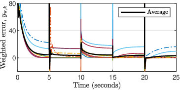
In this section, we demonstrate the coordination and robustness of the proposed control structure by means of a Matlab/Simulink simulation using Simscape components. We consider the network comprising 10 buses depicted in Fig. 2. In Section VII-A, we describe the setup of the simulation along with the various changes that the network is subjected to. Next, in Section VII-B, simulation results are presented for the case where Theorem 17 holds, i.e. with strictly passive loads and leaky agent PI controllers. Finally, in Section VII-C, we show the robust stability of the proposed control structure for passive loads and ideal agent PI controllers.

VII-A Simulation Setup

The DC microgrid in Fig. 2 is simulated with the parameters in Table I. The ZIP load parameters are chosen randomly in the specified ranges such that the required passivity measures are fulfilled (see 10). Furthermore, typical values are used for the DGUs and the lines [4, 9, 13]. The lines exhibit the same per kilometer parameter values and the line length are chosen randomly in the given interval. The line lengths are given in Appendix B.

TABLE I: Simulation Parameter Values


Voltages	${v}_{\mathrm{Ref}}=$	$380\text{\,}\mathrm{V}$	$v_{\mathrm{crit}}=$	$266\text{\,}\mathrm{V}$
DGU Filters (14)	$R_{k}=$	$0.2\text{\,}\mathrm{\SIUnitSymbolOhm}$	$L_{k}=$	$1.8\text{\,}\mathrm{mH}$
	$C_{k}=$	$2.2\text{\,}\mathrm{mF}$
ZIP Loads (III-A)	$\|Z^{-1}\|\leq$	$0.1\text{\,}\text{/}\mathrm{\SIUnitSymbolOhm}$	$\|I\>\!\|\leq$	$21\text{\,}\mathrm{A}$
	$\|P\,\|\leq$	$3\text{\,}\mathrm{kW}$
Elec. Lines (19)	$R_{kl}=$	$0.1\text{\,}\mathrm{\SIUnitSymbolOhm}\text{/}\mathrm{km}$	$L_{kl}=$	$2\text{\,}\mathrm{\SIUnitSymbolMicro H}\text{/}\mathrm{km}$
	$C_{kl}=$	$22\text{\,}\mathrm{nF}\text{/}\mathrm{km}$	length $\in$	$[0.2;10]\,$\mathrm{km}$$

TABLE II: Controller Parameter Values


Power PI Control (20)	$k_{\mathrm{d}}^{P}=$	$90$	$k_{\mathrm{d}}^{I}=$	$90$	$\tilde{R}=$	$-8$
DDA Control (24)	$k_{\mathrm{a}}^{P}=$	$50$	$k_{\mathrm{a}}^{I}=$	$100$	$\gamma_{\mathrm{a}}=$	$16$
Agent PI Control (27)	$k_{\mathrm{c}}^{P}=$	$160$	$k_{\mathrm{c}}^{I}=$		$\zeta_{\mathrm{c}}=$	$0.08$
Weighting Function (29)	$a_{\mathrm{w}}=$	$0.1$	$b_{\mathrm{w}}=$	$1.1$	$c_{\mathrm{w}}=$	$7.5\text{\,}\mathrm{V}$

The simulation starts off in State A (see Fig. 2) with Bus 9 connected and with all states at zero. The following changes are made at the indicated times.

•

$t=$5\text{\,}\mathrm{s}$$ : The actuation states $\alpha_{i}$ of the buses switches from State A to State B and Bus 9 is disconnected.
•

$t=$10\text{\,}\mathrm{s}$$ : The communication topology switches from State A to State B and Bus 10 is connected.
•

$t=$15\text{\,}\mathrm{s}$$ : The electrical topology switches from State A to State B.
•

$t=$20\text{\,}\mathrm{s}$$ : The bus actuation status along with the communication and electrical topologies revert to State A. Bus 9 is connected and Bus 10 is disconnected.

Furthermore, at each change, half of the buses are randomly selected and assigned new ZIP load parameters. The ZIP load parameters can be found in Appendix B.

The parameters for the closed-loop controller, as specified in Table II, are designed constructively, starting from the microgrid subsystems. First, the passivity indices for the lines ( $\rho_{\mathrm{t}}=0.01$ ) and loads ( $\rho_{\mathrm{L}}=\underline{c}_{\mathrm{L}}=0.05$ ) are calculated from Prop. 12 and Prop. 9, respectively. Next, the parameters for the power regulator (20) are chosen and the DGU passivity indices are calculated from Theorem 10, with the optimisation verified for the practically relevant intervals $\cramped{v\in[$200\text{\,}\mathrm{V}$,$550\text{\,}\mathrm{V}$]}$ and $\cramped{\hat{i}\in[$10\text{\,}\mathrm{A}$,$350\text{\,}\mathrm{A}$]}$ . Note that adding the restriction $\cramped{\nu_{\mathrm{d},2}\geq-\rho_{\mathrm{t}}}$ to the optimisation in Theorem 10 ensures that (54) will be met. This yields a solution $\nu_{\mathrm{d},1}=-4.686$ , $\nu_{\mathrm{d},2}=-0.01$ and $\rho_{\mathrm{d}}=0.01$ , from which the microgrid supply rate is constructed as per Theorem 14. Finally, parameters for the agent PI controllers are chosen and the weighting function parameters are designed using Theorem 17. Note that Theorem 14 requires strictly passive loads ( $\underline{c}_{\mathrm{L}}>0$ ) and Theorem 17 necessitates leaky integrators $(\cramped{\zeta_{\mathrm{c}}>0})$ .

VII-B Results

The bus voltages $v_{k}$ shown in Fig. 3 confirm the stability of the closed loop results, although the voltages tend to be lower than desired, due to the use of leaky integrators. The remaining steady-state offset can also be seen in the weighted errors plotted in Fig. 4, where the average tends towards a non-zero value in each instance (see 6). Despite this, the four stage controller reaches a consensus on the average of the nonlinear weighted voltage errors. Moreover, the advantage of the weighting function can be seen at Bus 6 in $t\in[$20\text{\,}\mathrm{s}$,$25\text{\,}\mathrm{s}$)$ , where a significant weighted error only appears in Fig. 4 when the voltage in Fig. 3 is not close to ${v}_{\mathrm{Ref}}$ . Note that the voltages of Buses 9 and 10 are at $0\text{\,}\mathrm{V}$ during the respective periods where they are disconnected and not actuated.

In Fig. 5, the outputs of the agent controllers show that no synchronisation of the agent controllers are required. The agent controller outputs at Buses 1 to 8, which are continuously connected to the communication network, are near identical. However, the disconnecting buses, e.g. Bus 9 after $t=$5\text{\,}\mathrm{s}$$ , rapidly diverge from other controllers and do not synchronise on reconnect. Despite this, the final stage of the controller ensures cooperation of the buses, as demonstrated in the power setpoints ${p}^{*}_{k}$ in Fig. 6. When Bus 10 connects at $t=$10\text{\,}\mathrm{s}$$ , its setpoint ${p}^{*}_{k}$ rapidly converges to the coordinated common setpoint used by all connected agents.

Although the leaky integrators yield imperfect results (see 6 and Fig. 4), this can be mitigated by choosing a higher ${v}_{\mathrm{Ref}}$ . Indeed, by combining the steady state of the agent PI controller (28) with the DDA steady state (25), we see that injecting power into the system ${\bm{p}}^{*}>0$ results in positive voltage errors. Since we consider (strictly) passive loads, increasing ${v}_{\mathrm{Ref}}$ is thus a viable method for correcting the imperfect results whilst retaining the advantageous properties of the stability analysis in Theorem 17.

VII-C Robustness Test

We now repeat the simulation described in Section VII-A with the following changes. 1) Passive loads with $\underline{c}_{\mathrm{L}}=0$ are allowed at all buses, and 2) ideal agent PI controllers with $\zeta_{\mathrm{c}}=0$ are used. Under these conditions, Theorem 17 can no longer be used to verify the stability. However, the stability may still be verified using classical approaches such as evaluating the eigenvalues for the closed loop linearised about the equilibrium. Note that the same random seed is used as for the results in Section VII-A, allowing for a comparison between the scenarios to be made.

Fig. 7demonstrates the improved consensus achieved by the ideal PI agents, in that the bus voltages are closer to ${v}_{\mathrm{Ref}}$ at steady state than in Fig. 3. Moreover, Fig. 8 shows that perfect consensus is achieved, where the average error tends to zero in each case. This figure also demonstrates the robustness against communication interruptions, as is the case for Bus 10 which, for the period $t\in[$5\text{\,}\mathrm{s}$,$10\text{\,}\mathrm{s}$)$ , is actuated but does not communicate with the other buses. Despite this, it is able to accurately regulate its own bus voltage (compared to the imperfect regulation achieved with leaky integrators as in Fig. 3). The lack of leaky integrators is also evident in Fig. 9, where the output of the agent controllers stay constant when a bus is disconnected and not actuated. Lastly, the power setpoints in Fig. 10 converging to a common value for the communicating agents confirm the coordination of the agents.

Note that while tests with non-passive loads can also yield a stable closed loop, instability can occur when the non-passive loads dominate. To address this, a targeted compensation of non-passive loads is required (see 11).

VIII Conclusion

In this paper, we proposed a four-stage distributed control structure that achieves power sharing in a DC microgrid while ensuring voltage regulation for the voltages of both actuated and unactuated buses. We demonstrated how the passivity properties of various subsystems can be determined and combined these in a stability analysis that is independent of topological changes, actuation changes, bus connections or disconnections and load changes.

Future work includes the consideration of non-passive loads at arbitrary locations in the microgrid and the construction of an interface to allow for the presented work to be combined with tertiary optimal controllers.

Appendix A Proofs

Proof of Prop. 8.

For the control structure in steady state, $\dot{\bm{x}}_{\mathrm{c}}=0$ and thus $\bm{y}_{\mathrm{c}}$ is constant. The steady-state output (25) of the Stage 4 DDA therefore ensures 2 is achieved. Furthermore, consider the steady state of the Stage 2 DDA

	$\displaystyle u_{\mathrm{a},s,k}$	$\displaystyle=\lim_{t\to\infty}h_{\mathrm{w}}({v}_{\mathrm{Ref}}-v_{k}),$		(81)
	$\displaystyle\lim_{t\to\infty}y_{\mathrm{a},2,k}$	$\displaystyle=\frac{\bm{u}_{\mathrm{a},s}^{T}\bm{\mathds{1}}_{N}}{N}=\lim_{t\to\infty}\frac{1}{N}\sum_{k\in\mathcal{N}}\left({v}_{\mathrm{Ref}}-h(v_{k})\right),$		(82)

if $v_{k}$ is in equilibrium and where $h$ is obtained by shifting $h_{\mathrm{w}}$ by ${v}_{\mathrm{Ref}}$ . Note that (82) corresponds to the condition of (22) in 1. Therefore, $\bm{y}_{\mathrm{a},2}$ specifies the regulation error of the average weighted voltage error in steady state. From the steady state of the agent PI controller in (27), we have $\zeta_{\mathrm{c}}\bm{x}_{\mathrm{c}}=\bm{y}_{\mathrm{a},2}$ . Thus, ideal integrators with $\zeta_{\mathrm{c}}=0$ ensure that 1 is met exactly. For $\zeta_{\mathrm{c}}>0$ , substitute the PI equilibrium into the output of the agent PI controller in (27) to obtain the steady state equation

\bm{x}_{\mathrm{c}}=\frac{1}{k_{\mathrm{c}}^{I}}\left(\bm{y}_{\mathrm{c}}+k_{\mathrm{c}}^{P}\bm{y}_{\mathrm{a},2}\right).

(83)

Substitute $\zeta_{\mathrm{c}}\bm{x}_{\mathrm{c}}=\bm{y}_{\mathrm{a},2}$ into (25) and simplify to find

\bm{y}_{\mathrm{a},2}=\frac{\zeta_{\mathrm{c}}}{k_{\mathrm{c}}^{I}(1+\zeta_{\mathrm{c}}k_{\mathrm{c}}^{P})}\bm{y}_{\mathrm{c}},

(84)

for the steady state. Since the entries of the vector $\bm{y}_{\mathrm{a},2}$ and thus of $\bm{x}_{\mathrm{c}}$ and $\bm{y}_{\mathrm{c}}$ are the same at steady state. Therefore the steady state output for the Stage 4 DDA in (25) gives $\bm{y}_{\mathrm{c}}=\bm{y}_{\mathrm{a},4}$ , which we combine with (84) to obtain the error for 1 in (30). ∎

Proof of Theorem 14.

Consider the supply rates which describe the actuated and unactuated states, respectively, for a given bus $k\in\mathcal{N}$

	$\displaystyle w_{\mathrm{M},\alpha,k}$	$\displaystyle=(1{+}\nu_{\mathrm{d},1}\rho_{\mathrm{d}}){\tilde{p}}^{}_{\alpha,k}\tilde{v}_{\alpha,k}-\nu_{\mathrm{d},1}{({\tilde{p}}^{}_{\alpha,k}{})}^{2}-\rho_{\mathrm{d}}\tilde{v}_{\alpha,k}^{2},\!\!$		(85)
	$\displaystyle w_{\mathrm{M},\beta,k}$	$\displaystyle=-\rho_{\mathrm{L}}\tilde{v}_{\beta,k}^{2}.$		(86)

These allow the microgrid supply rate in (49) to be decomposed according to the actuation states $\alpha_{k}$

	$\displaystyle w_{\mathrm{M},\alpha\beta}=$	$\displaystyle\sum_{k\in\mathcal{N}_{\alpha}}w_{\mathrm{M},\alpha,k}+\sum_{k\in\mathcal{N}_{\beta}}w_{\mathrm{M},\beta,k}$		(87)
	$\displaystyle=$	$\displaystyle\sum_{k\in\mathcal{N}}\left(\alpha_{k}w_{\mathrm{M},\alpha,k}+(1-\alpha_{k})w_{\mathrm{M},\beta,k}\right)$		(87)

Enlarge the supply rate of the unactuated buses in (86) by adding the positive term $\nu_{\mathrm{L}}{({\tilde{p}}^{*}_{\beta,k}{})}^{2}$ for an arbitrarily small $\nu_{\mathrm{L}}>0$ such that

	$\displaystyle w_{\mathrm{M},\beta,k}$	$\displaystyle\leq\overline{w}_{\mathrm{M},\beta,k}\,=\,\nu_{\mathrm{L}}{({\tilde{p}}^{*}_{\beta,k}{})}^{2}-\rho_{\mathrm{L}}\tilde{v}_{\beta,k}^{2}$		(88)
		$\displaystyle\leq\frac{\overline{w}_{\mathrm{M},\beta,k}}{\rho_{\mathrm{L}}}=\frac{\nu_{\mathrm{L}}}{\rho_{\mathrm{L}}}{({\tilde{p}}^{*}_{\beta,k}{})}^{2}-\tilde{v}_{\beta,k}^{2}$		(88)

for $\rho_{\mathrm{L}}$ as in (55). The supply rate $\overline{w}_{\mathrm{M},\beta,k}/\rho_{\mathrm{L}}$ is equivalent to the $L_{2}$ supply rate in 2 and is thus bounded by the sector $[-\sqrt{\frac{\nu_{\mathrm{L}}}{\rho_{\mathrm{L}}}},\sqrt{\frac{\nu_{\mathrm{L}}}{\rho_{\mathrm{L}}}}]$ [29, Lemma 4]. Consider now the supply rate of the actuated agents (85) narrowed down to an IFP sector for the case that $\rho_{\mathrm{d}}<0$ , i.e.

w_{\mathrm{M},\alpha,k}\geq\underline{w}_{\mathrm{M},\alpha,k}=\left\{\begin{aligned} &w_{\mathrm{M},\alpha,k},\!\quad&&\text{if}\;\;\rho_{\mathrm{d}}\geq 0,\\ &{\tilde{p}}^{*}_{\alpha,k}\tilde{v}_{\alpha,k}-\nu_{\mathrm{d},1}{({\tilde{p}}^{*}_{\alpha,k}{})}^{2},\!\quad&&\text{if}\;\;\rho_{\mathrm{d}}<0,\end{aligned}\right.

(89)

such that $\underline{w}_{\mathrm{M},\alpha,k}$ is sector bounded by $[\nu_{\mathrm{d},1},\frac{1}{\rho_{\mathrm{d}}}]$ if $\rho_{\mathrm{d}}>0$ and $[\nu_{\mathrm{d},1},\infty)$ if $\rho_{\mathrm{d}}<0$ or if $\rho_{\mathrm{d}}=0$ (see [26, p. 231]). A relation bewteen $\underline{w}_{\mathrm{M},\alpha}$ and $\overline{w}_{\mathrm{M},\beta}/\rho_{\mathrm{L}}$ can now be established by comparing their respective sector bounds:

\frac{\overline{w}_{\mathrm{M},\beta,k}}{\rho_{\mathrm{L}}}\leq\underline{w}_{\mathrm{M},\alpha,k}\;\text{if}\left\{\begin{aligned} &[-\sqrt{\tfrac{\nu_{\mathrm{L}}}{\rho_{\mathrm{L}}}},\sqrt{\tfrac{\nu_{\mathrm{L}}}{\rho_{\mathrm{L}}}}]\subseteq[\nu_{\mathrm{d},1},\tfrac{1}{\rho_{\mathrm{d}}}],\!\!\!&\text{if}\;\rho_{\mathrm{d}}>0,\\ &[-\sqrt{\tfrac{\nu_{\mathrm{L}}}{\rho_{\mathrm{L}}}},\sqrt{\tfrac{\nu_{\mathrm{L}}}{\rho_{\mathrm{L}}}}]\subseteq[\nu_{\mathrm{d},1},\infty),\!\!\!&\text{if}\;\rho_{\mathrm{d}}\leq 0,\end{aligned}\right.

(90)

Fig. 11: Comparison of the microgrid supply rate sectors in the proof of Theorem 14 if

\rho_{\mathrm{d}}<0

Since $\nu_{\mathrm{L}}$ can be arbitrarily small, we derive (56) by comparing the lower bounds in (90) and note that the upper bound relation can be met for any $\rho_{\mathrm{d}}$ . A visual comparison of the sector conditions is made in Fig. 11. The combination of (88)–(90) results in

w_{\mathrm{M},\beta,k}\leq\overline{w}_{\mathrm{M},\beta,k}\leq\frac{\overline{w}_{\mathrm{M},\beta,k}}{\rho_{\mathrm{L}}}\leq\underline{w}_{\mathrm{M},\alpha,k}\leq w_{\mathrm{M},\alpha,k}.

(91)

Therefore, for the microgrid with the storage function $S_{\mathrm{M}}$ that is dissipative w.r.t. (49), it holds that

\displaystyle\dot{S}_{\mathrm{M}}\leq w_{\mathrm{M},\alpha\beta}\leq\sum_{k\in\mathcal{N}}w_{\mathrm{M},\alpha,k}=w_{\mathrm{M}},

(92)

which is found by combining (87) with (91). ∎

Appendix B Simulation Data

The simulation parameters used for the lines in Section VII are given in Table III. Furthermore, the strictly passive load parameters for the simulation results in Section VII-B and the passive load parameters for the results in Section VII-C are given in Table IV and Table V, respectively. Note that the $P$ parameter for the loads in Table V are the same as listed in Table IV.

TABLE III: Rounded Line Lengths

Line	Length	Line	Length	Line	Length

1 – 2	$1.19\text{\,}\mathrm{km}$	1 – 4	$7.74\text{\,}\mathrm{km}$	2 – 3	$2.23\text{\,}\mathrm{km}$
2 – 4	$7.20\text{\,}\mathrm{km}$	3 – 5	$3.14\text{\,}\mathrm{km}$	3 – 8	$2.82\text{\,}\mathrm{km}$
4 – 5	$3.72\text{\,}\mathrm{km}$	4 – 6	$6.75\text{\,}\mathrm{km}$	4 – 7	$1.16\text{\,}\mathrm{km}$
6 – 7	$4.44\text{\,}\mathrm{km}$	6 – 9	$3.11\text{\,}\mathrm{km}$	7 – 8	$3.69\text{\,}\mathrm{km}$
8 – 10	$1.21\text{\,}\mathrm{km}$

TABLE IV: Strictly Passive Load Values


Bus	Parameter	$t=$0\text{\,}\mathrm{s}$$	$t=$5\text{\,}\mathrm{s}$$	$t=$10\text{\,}\mathrm{s}$$	$t=$15\text{\,}\mathrm{s}$$	$t=$20\text{\,}\mathrm{s}$$

	$Z^{-1}$ $($\text{/}\mathrm{\SIUnitSymbolOhm}$)$	0.103	0.103	0.106	0.106	0.083
1	$I$ $($\mathrm{A}$)$	4.66	2.15	-6.08	-6.08	14.45
	$P$ $($\mathrm{W}$)$	3599	-4055	4133	4133	-4927
	$Z^{-1}$ $($\text{/}\mathrm{\SIUnitSymbolOhm}$)$	0.099	0.099	0.096	0.096	0.080
2	$I$ $($\mathrm{A}$)$	-16.09	-16.09	19.68	19.68	2.49
	$P$ $($\mathrm{W}$)$	3204	3204	2659	2659	1346
	$Z^{-1}$ $($\text{/}\mathrm{\SIUnitSymbolOhm}$)$	0.128	0.105	0.105	0.105	0.096
3	$I$ $($\mathrm{A}$)$	10.27	-0.09	-0.09	-0.09	-11.09
	$P$ $($\mathrm{W}$)$	-1479	-3659	-3659	-3659	3031
	$Z^{-1}$ $($\text{/}\mathrm{\SIUnitSymbolOhm}$)$	0.079	0.079	0.079	0.079	0.079
4	$I$ $($\mathrm{A}$)$	10.15	10.15	10.15	10.15	10.15
	$P$ $($\mathrm{W}$)$	-2711	-2711	-2711	-2711	-2711
	$Z^{-1}$ $($\text{/}\mathrm{\SIUnitSymbolOhm}$)$	0.095	0.095	0.095	0.064	0.107
5	$I$ $($\mathrm{A}$)$	-6.64	-6.64	-6.64	16.68	2.10
	$P$ $($\mathrm{W}$)$	2768	2768	2768	-3798	4242
	$Z^{-1}$ $($\text{/}\mathrm{\SIUnitSymbolOhm}$)$	0.089	0.089	0.106	0.103	0.103
6	$I$ $($\mathrm{A}$)$	6.87	6.87	7.85	-5.17	-5.17
	$P$ $($\mathrm{W}$)$	948	948	4321	370	370
	$Z^{-1}$ $($\text{/}\mathrm{\SIUnitSymbolOhm}$)$	0.065	0.092	0.092	0.118	0.118
7	$I$ $($\mathrm{A}$)$	11.96	6.51	6.51	2.77	2.77
	$P$ $($\mathrm{W}$)$	-3624	-3442	-3442	-3890	-3890
	$Z^{-1}$ $($\text{/}\mathrm{\SIUnitSymbolOhm}$)$	0.102	0.102	0.086	0.086	0.124
8	$I$ $($\mathrm{A}$)$	-16.85	-16.85	20.71	20.71	-4.68
	$P$ $($\mathrm{W}$)$	3529	3529	-4773	-4773	-3832
	$Z^{-1}$ $($\text{/}\mathrm{\SIUnitSymbolOhm}$)$	0.111	0.103	0.109	0.077	0.077
9	$I$ $($\mathrm{A}$)$	13.79	-19.74	9.53	1.26	1.26
	$P$ $($\mathrm{W}$)$	-2645	1830	4215	1549	1549
	$Z^{-1}$ $($\text{/}\mathrm{\SIUnitSymbolOhm}$)$	0.072	0.100	0.100	0.111	0.111
10	$I$ $($\mathrm{A}$)$	7.77	9.02	9.02	10.98	10.98
	$P$ $($\mathrm{W}$)$	-3538	-4143	-4143	-2795	-2795

TABLE V: Passive Load Values,

P

as in Table IV


Bus	Parameter	$t=$0\text{\,}\mathrm{s}$$	$t=$5\text{\,}\mathrm{s}$$	$t=$10\text{\,}\mathrm{s}$$	$t=$15\text{\,}\mathrm{s}$$	$t=$20\text{\,}\mathrm{s}$$

1	$Z^{-1}$ $($\text{/}\mathrm{\SIUnitSymbolOhm}$)$	0.091	0.093	0.087	0.087	0.063
	$I$ $($\mathrm{A}$)$	4.66	-8.15	-6.08	-6.08	9.71
2	$Z^{-1}$ $($\text{/}\mathrm{\SIUnitSymbolOhm}$)$	0.069	0.069	0.071	0.071	0.046
	$I$ $($\mathrm{A}$)$	-16.09	-16.09	19.68	19.68	0.20
3	$Z^{-1}$ $($\text{/}\mathrm{\SIUnitSymbolOhm}$)$	0.095	0.082	0.082	0.082	0.059
	$I$ $($\mathrm{A}$)$	8.91	-7.12	-7.12	-7.12	-11.09
4	$Z^{-1}$ $($\text{/}\mathrm{\SIUnitSymbolOhm}$)$	0.038	0.038	0.038	0.038	0.038
	$I$ $($\mathrm{A}$)$	8.82	8.82	8.82	8.82	8.82
5	$Z^{-1}$ $($\text{/}\mathrm{\SIUnitSymbolOhm}$)$	0.065	0.065	0.065	0.027	0.078
	$I$ $($\mathrm{A}$)$	-6.64	-6.64	-6.64	15.25	2.10
6	$Z^{-1}$ $($\text{/}\mathrm{\SIUnitSymbolOhm}$)$	0.071	0.071	0.089	0.102	0.102
	$I$ $($\mathrm{A}$)$	4.04	4.04	7.85	-9.19	-9.19
7	$Z^{-1}$ $($\text{/}\mathrm{\SIUnitSymbolOhm}$)$	0.029	0.070	0.070	0.079	0.079
	$I$ $($\mathrm{A}$)$	9.04	0.89	0.89	0.58	0.58
8	$Z^{-1}$ $($\text{/}\mathrm{\SIUnitSymbolOhm}$)$	0.075	0.075	0.057	0.057	0.111
	$I$ $($\mathrm{A}$)$	-16.85	-16.85	20.55	20.55	-14.31
9	$Z^{-1}$ $($\text{/}\mathrm{\SIUnitSymbolOhm}$)$	0.105	0.102	0.061	0.036	0.036
	$I$ $($\mathrm{A}$)$	10.71	-19.75	9.53	-0.05	-0.05
10	$Z^{-1}$ $($\text{/}\mathrm{\SIUnitSymbolOhm}$)$	0.042	0.091	0.091	0.088	0.088
	$I$ $($\mathrm{A}$)$	2.53	2.03	2.03	8.34	8.34

References

[1] B. Lasseter, “Microgrids [distributed power generation],” in Proc. 2001 IEEE Power Engineering Society Winter Meeting, vol. 1, 2001, pp. 146–149.
[2] J. J. Justo, F. Mwasilu, J. Lee, and J.-W. Jung, “AC-microgrids versus DC-microgrids with distributed energy resources: A review,” Renewable and Sustainable Energy Reviews, vol. 24, pp. 387–405, 2013.
[3] L. Meng, Q. Shafiee, G. F. Trecate, H. Karimi, D. Fulwani, X. Lu, and J. M. Guerrero, “Review on control of DC microgrids and multiple microgrid clusters,” IEEE J. of Emerging and Selected Topics in Power Electron., vol. 5, no. 3, pp. 928–948, 2017.
[4] V. Nasirian, S. Moayedi, A. Davoudi, and F. L. Lewis, “Distributed cooperative control of DC microgrids,” IEEE Trans. Power Electron., vol. 30, no. 4, pp. 2288–2303, 2015.
[5] M. Tucci, L. Meng, J. M. Guerrero, and G. Ferrari-Trecate, “Stable current sharing and voltage balancing in DC microgrids: A consensus-based secondary control layer,” Automatica, vol. 95, pp. 1–13, 2018.
[6] J. Zhao and F. Dörfler, “Distributed control and optimization in dc microgrids,” Automatica, vol. 61, pp. 18–26, 2015.
[7] T. Dragičević, X. Lu, J. C. Vasquez, and J. M. Guerrero, “DC microgrids—part i: A review of control strategies and stabilization techniques,” IEEE Trans. Power Electron., vol. 31, no. 7, pp. 4876–4891, 2016.
[8] J. Kumar, A. Agarwal, and V. Agarwal, “A review on overall control of dc microgrids,” J. of Energy Storage, vol. 21, pp. 113–138, 2019.
[9] M. Tucci, S. Riverso, J. C. Vasquez, J. M. Guerrero, and G. Ferrari-Trecate, “A decentralized scalable approach to voltage control of DC islanded microgrids,” IEEE Trans. Control Syst. Technol., vol. 24, no. 6, pp. 1965–1979, 2016.
[10] F. Strehle, M. Pfeifer, A. J. Malan, S. Krebs, and S. Hohmann, “A scalable port-Hamiltonian approach to plug-and-play voltage stabilization in DC microgrids,” in 2020 IEEE Conf. Control Technol. and Applications, 2020, pp. 787–794.
[11] M. Cucuzzella, K. C. Kosaraju, and J. M. A. Scherpen, “Voltage control of DC microgrids: Robustness for unknown ZIP-loads,” IEEE Control Syst. Lett., vol. 7, pp. 139–144, 2023.
[12] S. Trip, M. Cucuzzella, X. Cheng, and J. Scherpen, “Distributed averaging control for voltage regulation and current sharing in DC microgrids,” IEEE Control Syst. Lett., vol. 3, no. 1, pp. 174–179, 2019.
[13] M. Cucuzzella, S. Trip, C. De Persis, X. Cheng, A. Ferrara, and A. van der Schaft, “A robust consensus algorithm for current sharing and voltage regulation in DC microgrids,” IEEE Trans. Control Syst. Technol., vol. 27, no. 4, pp. 1583–1595, 2019.
[14] M. S. Sadabadi, S. Sahoo, and F. Blaabjerg, “Stability-oriented design of cyberattack-resilient controllers for cooperative DC microgrids,” IEEE Trans. Power Electron., vol. 37, no. 2, pp. 1310–1321, 2022.
[15] R. Han, L. Meng, J. M. Guerrero, and J. C. Vasquez, “Distributed nonlinear control with event-triggered communication to achieve current-sharing and voltage regulation in DC microgrids,” IEEE Trans. Power Electron., vol. 33, no. 7, pp. 6416–6433, 2018.
[16] P. Nahata and G. Ferrari-Trecate, “On existence of equilibria, voltage balancing, and current sharing in consensus-based DC microgrids,” in Proc. Eur. Control Conf. (ECC), 2020, pp. 1216–1223.
[17] P. Nahata, M. S. Turan, and G. Ferrari-Trecate, “Consensus-based current sharing and voltage balancing in dc microgrids with exponential loads,” IEEE Trans. Control Syst. Technol., vol. 30, no. 4, pp. 1668–1680, 2022.
[18] C. De Persis, E. Weitenberg, and F. Dörfler, “A power consensus algorithm for DC microgrids,” IFAC-PapersOnLine, vol. 50, no. 1, pp. 10 009–10 014, 2017, 20th IFAC World Congress.
[19] B. Fan, S. Guo, J. Peng, Q. Yang, W. Liu, and L. Liu, “A consensus-based algorithm for power sharing and voltage regulation in dc microgrids,” IEEE Trans. Ind. Inform., vol. 16, no. 6, pp. 3987–3996, 2020.
[20] M. Cucuzzella, K. C. Kosaraju, and J. M. A. Scherpen, “Distributed passivity-based control of DC microgrids,” in American Control Conf. (ACC), 2019, pp. 652–657.
[21] F. Dörfler and F. Bullo, “Kron reduction of graphs with applications to electrical networks,” IEEE Trans. Circuits Syst., vol. 60, no. 1, pp. 150–163, 2013.
[22] W. Chen, D. Wang, J. Liu, Y. Chen, S. Z. Khong, T. Başar, K. H. Johansson, and L. Qiu, “On spectral properties of signed laplacians with connections to eventual positivity,” IEEE Trans. Autom. Control, vol. 66, no. 5, pp. 2177–2190, 2021.
[23] A. J. Malan, M. Pfeifer, and S. Hohmann, “Distributed coordination of physically-interconnected multi-agent systems with actuated and unactuated agents,” Eur. J. Control, p. 100673, 2022.
[24] A. J. van der Schaft, L2-Gain and Passivity Techniques in Nonlinear Control, 3rd ed. Cham, Switzerland: Springer, 2017.
[25] M. Arcak and E. D. Sontag, “Diagonal stability of a class of cyclic systems and its connection with the secant criterion,” Automatica, vol. 42, no. 9, pp. 1531–1537, 2006.
[26] H. K. Khalil, Nonlinear Systems, 3rd ed. Upper Saddle River, NJ: Prentice Hall, 2002.
[27] G. H. H. Hines, M. Arcak, and A. K. Packard, “Equilibrium-independent passivity: A new definition and numerical certification,” Automatica, vol. 47, no. 9, pp. 1949–1956, 2011.
[28] M. Arcak, C. Meissen, and A. Packard, Networks of Dissipative Systems: Compositional Certification of Stability, Performance, and Safety, ser. (SpringerBriefs in Control, Automation and Robotics). New York, NY, USA: Springer, 2016.
[29] A. J. Malan, P. Jané-Soneira, and S. Hohmann, “Constructive analysis and design of interconnected krasovskii passive and quadratic dissipative systems,” in Proc. 61th IEEE Conf. Decis. Control (CDC), 2022.
[30] P. Moylan and D. Hill, “Stability criteria for large-scale systems,” IEEE Trans. Autom. Control, vol. 23, no. 2, pp. 143–149, 1978.
[31] M. Benzi, G. H. Golub, and J. Liesen, “Numerical solution of saddle point problems,” Acta Numerica, vol. 14, p. 1–137, 2005.
[32] F. Strehle, A. J. Malan, S. Krebs, and S. Hohmann, “Passivity conditions for plug-and-play operation of nonlinear static AC loads,” IFAC-PapersOnLine, vol. 53, no. 2, pp. 12 237–12 243, 2020, 21st IFAC World Congress.
[33] J. Machowski, J. W. Bialek, and J. R. Bumby, Power System Dynamics: Stability and Control, 2nd ed. Chichester, United Kingdom: John Wiley & Sons, Ltd., 2008.
[34] R. A. Freeman, P. Yang, and K. M. Lynch, “Stability and convergence properties of dynamic average consensus estimators,” in Proc. 45th IEEE Conf. Decis. Control (CDC), 2006, pp. 338–343.
[35] E. Weitenberg, Y. Jiang, C. Zhao, E. Mallada, F. Dörfler, and C. De Persis, “Robust decentralized frequency control: A leaky integrator approach,” in Proc. Eur. Control Conf. (ECC), 2018, pp. 764–769.
[36] T. Raff, C. Ebenbauer, and P. Allgöwer, Nonlinear Model Predictive Control: A Passivity-Based Approach. Berlin, Heidelberg: Springer, 2007, pp. 151–162.