Effects of calibration uncertainties on the detection and parameter estimation of isotropic gravitational-wave backgrounds
Abstract
Gravitational-wave backgrounds are expected to arise from the superposition of gravitational wave signals from a large number of unresolved sources and also from the stochastic processes that occurred in the Early universe. So far, we have not detected any gravitational wave background, but with the improvements in the detectors’ sensitivities, such detection is expected in the near future. The detection and inferences we draw from the search for a gravitational-wave background will depend on the source model, the type of search pipeline used, and the data generation in the gravitational-wave detectors. In this work, we focus on the effect of the data generation process, specifically the calibration of the detectors’ digital output into strain data used by the search pipelines. Using the calibration model of the current LIGO detectors as an example, we show that for power-law source models and calibration uncertainties , the detection of isotropic gravitational wave background is not significantly affected. We also show that the source parameter estimation and upper limits calculations get biased. For calibration uncertainties of , the biases are not significant (), but for larger calibration uncertainties, they might become significant, especially when trying to differentiate between different models of isotropic gravitational-wave backgrounds.
I Introduction
Since the first detection in September 2015 Abbott et al. 2016a, the LIGO Aasi et al. 2015a, and the Virgo Acernese et al. 2015 gravitational wave (GW) detectors have detected nearly one-hundred compact binary merger signals Abbott et al. 2019a; Abbott et al. 2021a; Abbott et al. 2021b. They correspond to individual merger signals with a high signal-to-noise ratio (SNR). In addition to those high SNR signals, assuming the merger events are outliers in a much larger population of compact mergers, we also expect many low SNR signals that are hard to detect individually. The superposition of such a large number of low SNR signals would give rise to a gravitational-wave background (GWB) that could be detected with the current or next generation of GW detectors Abbott et al. 2016b; Abbott et al. 2018; Abbott et al. 2021c; Regimbau 2022.
Apart from the compact binary mergers signals, superposition of other astrophysical GW signals such as from core-collapse supernovae Buonanno et al. 2005; Howell et al. 2004, magnetars Rosado 2012; Zhu et al. 2011 could also give rise to GWB. In addition to these astrophysical sources, various events that took place in the early universe such as inflation and phase transitions could also give rise to GWB Caprini and Figueroa 2018. The detection of GWB from astrophysical sources can help us better understand the population and the evolution of stars in the universe Regimbau 2011; de Freitas Pacheco 2020; Romano and Cornish 2017 while the detection of GWB from cosmological sources can provide information about the processes in the very early universe which are otherwise difficult to obtain Maggiore 2000.
The LIGO-Virgo-KAGRA (LVK) collaboration, in their recent analyses using data from the observing run O3, did not find any evidence of GWBs and hence placed upper limits on the amplitudes of possible isotropic Abbott et al. 2021d and anisotropic GWBs Abbott et al. 2021e. With the proposed improvements to the current GW detectors Abbott et al. 2020, it might be possible to detect the GWB from compact binary mergers Regimbau 2022. Also, the proposed next-generation GW detectors Reitze et al. 2019; Punturo et al. 2010 are expected to observe the GWB from compact binary mergers with high SNRs Périgois et al. 2021; Regimbau et al. 2017. The data generation and various aspects of the search are expected to affect the GWB search results, and hence it is important to understand them. In this paper, we focus on the effects of the data generation, specifically that of the calibration, on the analysis results. Calibration is the process of converting the raw digital outputs of the detectors into strain data that are further used in the GW analyses. Any uncertainties in that process could translate into biases and larger uncertainties in the final results, affecting our interpretations.
Typically, cross-correlation-based searches correlating data from multiple detectors are used to detect GWBs Allen and Romano 1999. In previous such searches using LIGO-Virgo data Abbott et al. 2017; Abbott et al. 2019b; Abbott et al. 2021d, upper limits were calculated after marginalizing over calibration uncertainties as outlined in Whelan et al. 2014. However, that method does not capture any biases introduced by uncertainties and systematic errors in the calibration model. In this work, we try to address that issue. In the past, this has been studied primarily in the context of the search for GW signals from individual compact binaries Allen 1996; Vitale et al. 2012; Farr et al. 2014; Hall et al. 2019. Recently, such questions have also been addressed for the detection and parameter estimation of individual compact binary merger signals Payne et al. 2020; Vitale et al. 2021; Essick 2022. We use a similar simulation-based method Payne et al. 2020; Vitale et al. 2021 to address the effects of calibration uncertainties on the searches for GWB. In addition, we also show that one could try to estimate the GWB and calibration model parameters simultaneously and get a reasonable signal recovery.
The remainder of this paper is organized as follows. In Sec. II, we briefly introduce the model and search for GWB using data from GW detectors. In Sec. III, we discuss the calibration model used to convert the raw digital output into strain data used in GW searches. In Sec. IV, we describe the method used to quantify the effects of calibration uncertainties on the isotropic GWB searches. In Sec. V, we show the results of our analyses, and in Sec. VI conclude with the main results and future outlook.
II Modeling and search for isotropic gravitational-wave backgrounds
An isotropic GWB is usually characterized in terms of fractional energy density in gravitational waves Allen and Romano 1999, given by,
| (1) |
where is the frequency, is the energy in gravitational waves in the frequency interval from to , is the critical energy density needed to close the universe. The value of is given by
| (2) |
where is the speed of light, is the gravitational constant and is the Hubble constant. In this work, we use the value of Hubble constant measured by the Plank satellite, (Ade et al. 2016). However, the conclusions drawn are independent of the actual value of .
Typically is expressed in the form of a power law,
| (3) |
where is a reference frequency. For results reported in this paper, we use a reference frequency of as used in the LVK analyses (Abbott et al. 2017; Abbott et al. 2019b; Abbott et al. 2021d). The value of the power-law index depends on the source of GWB we are interested in. For cosmological GWB from inflationary scenarios, we typically expect Caprini and Figueroa 2018 while for astrophysical GWB from the superposition of many compact binary mergers signals Regimbau 2011. Similar to LVK analyses (Abbott et al. 2017; Abbott et al. 2019b; Abbott et al. 2021d), in addition to and , we also look at representing astrophysical GWB models such as from supernovae Sandick et al. 2006.
Instead of searching for , traditionally, isotropic GWB searches try to estimate for different values of power-law index . The optimal estimator of , for an isotropic GWB, at a time and at a frequency bin is given by Aasi et al. 2015b; Romano and Cornish 2017,
| (4) |
where and are short-time Fourier transforms of the strain data from the two detectors evaluated at time , is the duration of the data segments used for Fourier transforms and is the normalized overlap reduction function for the given two detectors . The function is proportional to the assumed spectral shape and is given by (Aasi et al. 2015b; Romano and Cornish 2017),
| (5) |
In the weak-signal limit, the variance of is given by Aasi et al. 2015b; Romano and Cornish 2017,
| (6) |
where , are the one-sided power spectral densities of the strain data from the two detectors , and is the frequency resolution. For data spanning many segments and a large frequency band, the final optimal estimators are obtained by a weighted sum,
| (7) |
where runs over available time segments and runs over discrete frequency bins in the desired frequency band.
III Calibration Model
The raw outputs of gravitational wave detectors are digitized electrical signals from the photodetectors at the output port. The process of converting these electrical signals into strain data is called . The LIGO, Virgo, and KAGRA detectors have similar fundamentals in optical layout and control system topology Aasi et al. 2015a; Acernese et al. 2015; Akutsu et al. 2021a. While their methods to describe and characterize that system are different (sometimes only in subtle ways that reflect their detailed differences), any of those methods could be used to describe current GW detectors. Thus, here, we follow and choose the methods of the LIGO detectors Abbott et al. 2017; Sun et al. 2020. For details of different calibration techniques used in the current generation of gravitational wave detectors, see Abbott et al. 2017; Viets et al. 2018; Acernese et al. 2022; Akutsu et al. 2021b. As shown in Sun et al. 2020, after detailed modeling of the detectors, a response function is derived, which is then used to convert the digitized electrical output into strain using the expression,
| (8) |
where e(f) is the digitized signals from the output photo-detectors, R(f) is the response function that converts e(f) into the differential displacement of the two arms of the detector and L is the average (macroscopic) length of the two arms.
The response function of a gravitational wave detector, in the frequency domain, can be written as Sun et al. 2020,
| (9) |
where is the sensing function corresponding to the response of the detector to differential changes in its two arms without any feedback control, is the actuation function used to control the positions of the mirrors and is any digital filter(s) used in the control loop.
III.1 Sensing function
The sensing function can be modeled in the frequency domain as Cahillane et al. 2017; Sun et al. 2020,
| (10) | |||||
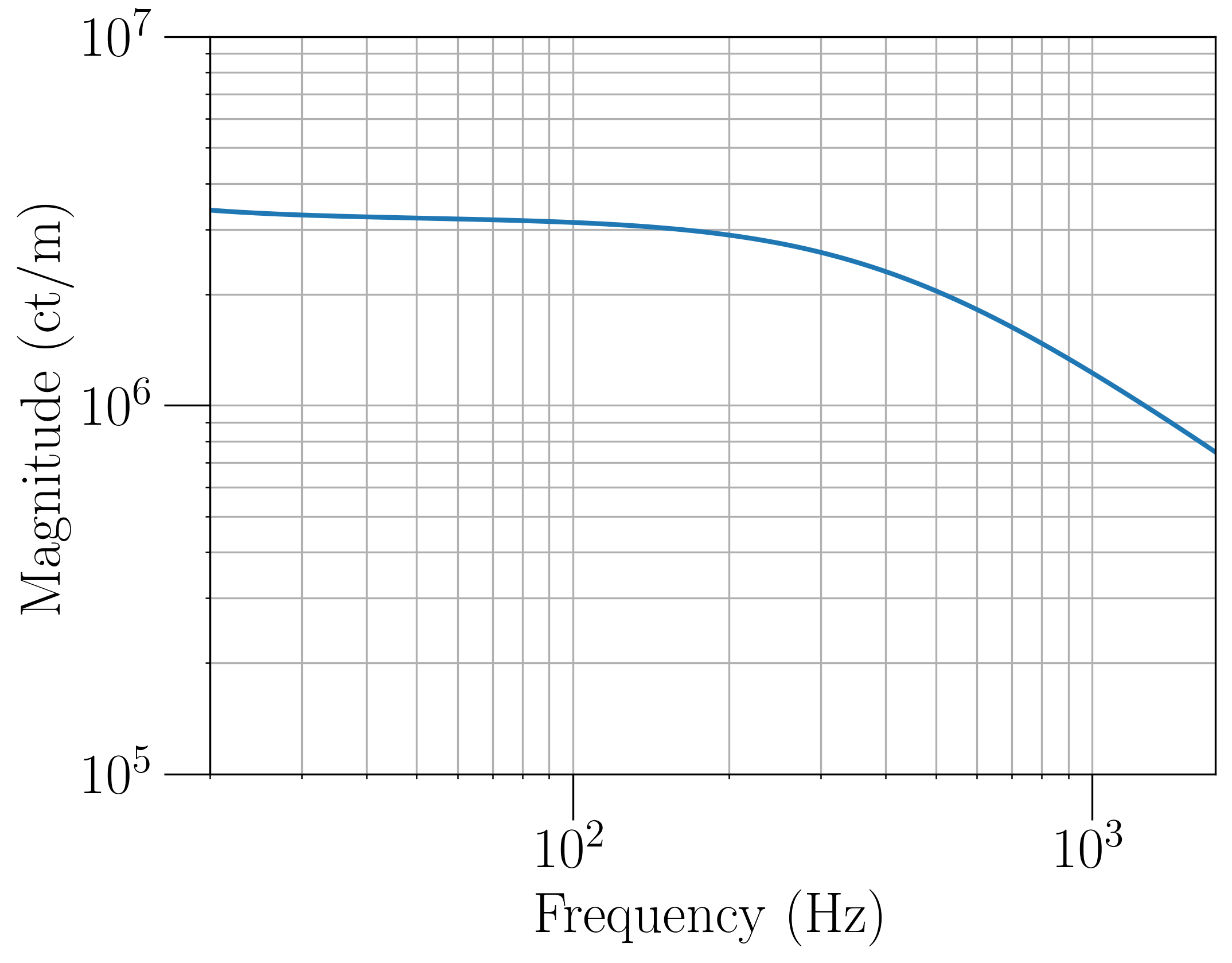
where optical gain represents the overall gain, coupled-cavity pole frequency defines the detector bandwidth, and correspond to optical anti-spring pole frequency and its quality factor, respectively. The term represents the frequency dependencies not captured by the other terms (for example, the response of the electronics chain used for the digitization, etc.), and is a scale factor representing the changes in the sensing function with respect to a reference time. The sensing function we use in our analysis is shown in Fig. 1. We use the pyDARM package pyd to generate the calibration model used in this work.
For LIGO detectors, during the past observing runs and for frequencies Hz, the optical spring term (second term in Eq. 10) was usually close to one (for example, see lho; llo). Since in our work, we use Hz band as done in LVK analyses Abbott et al. 2017; Abbott et al. 2019b; Abbott et al. 2021d, we treat the optical spring term in Eq. 10 as constant and do not study its effects in this work.
III.2 Actuation function
The actuation function is modeled in the frequency domain as Cahillane et al. 2017; Sun et al. 2020,
| (11) |
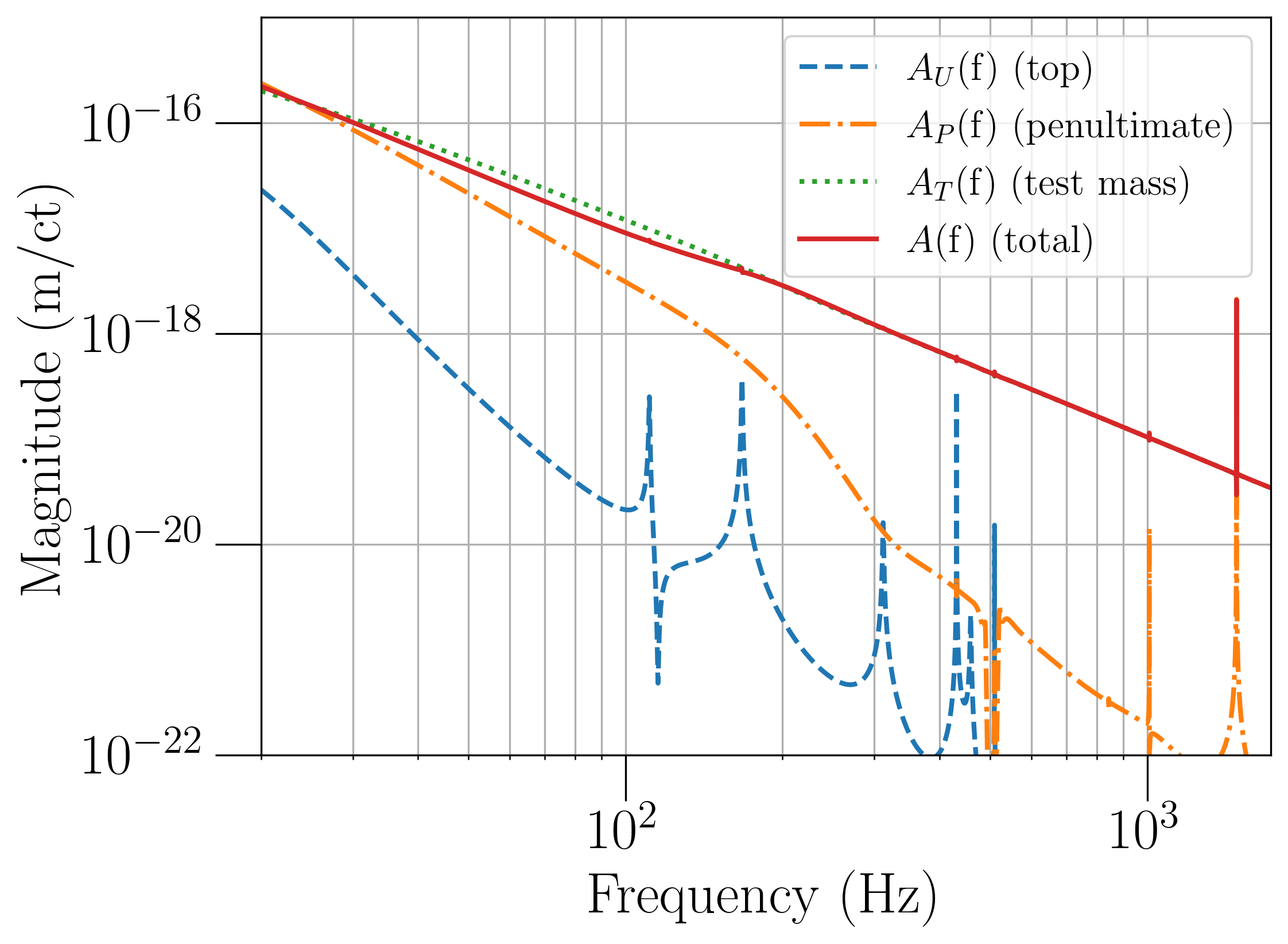
where , , and represent the lowest three stages of suspensions (upper intermediate mass, penultimate, and test mass stages) used to suspend the main optics Aasi et al. 2015a; Sun et al. 2020. (where ) are frequency-dependent actuation models of the three stages of the suspensions, including digital filters in the control path and analog responses of the three stages of suspensions Sun et al. 2020. The scale factors capture any changes in the reference actuation model of each stage, and in general, they could be time- and frequency-dependent Tuyenbayev et al. 2016. The plots of actuation models for the three stages and the combined actuation model used in this work are shown in Fig. 2.
III.3 Interferometer response function
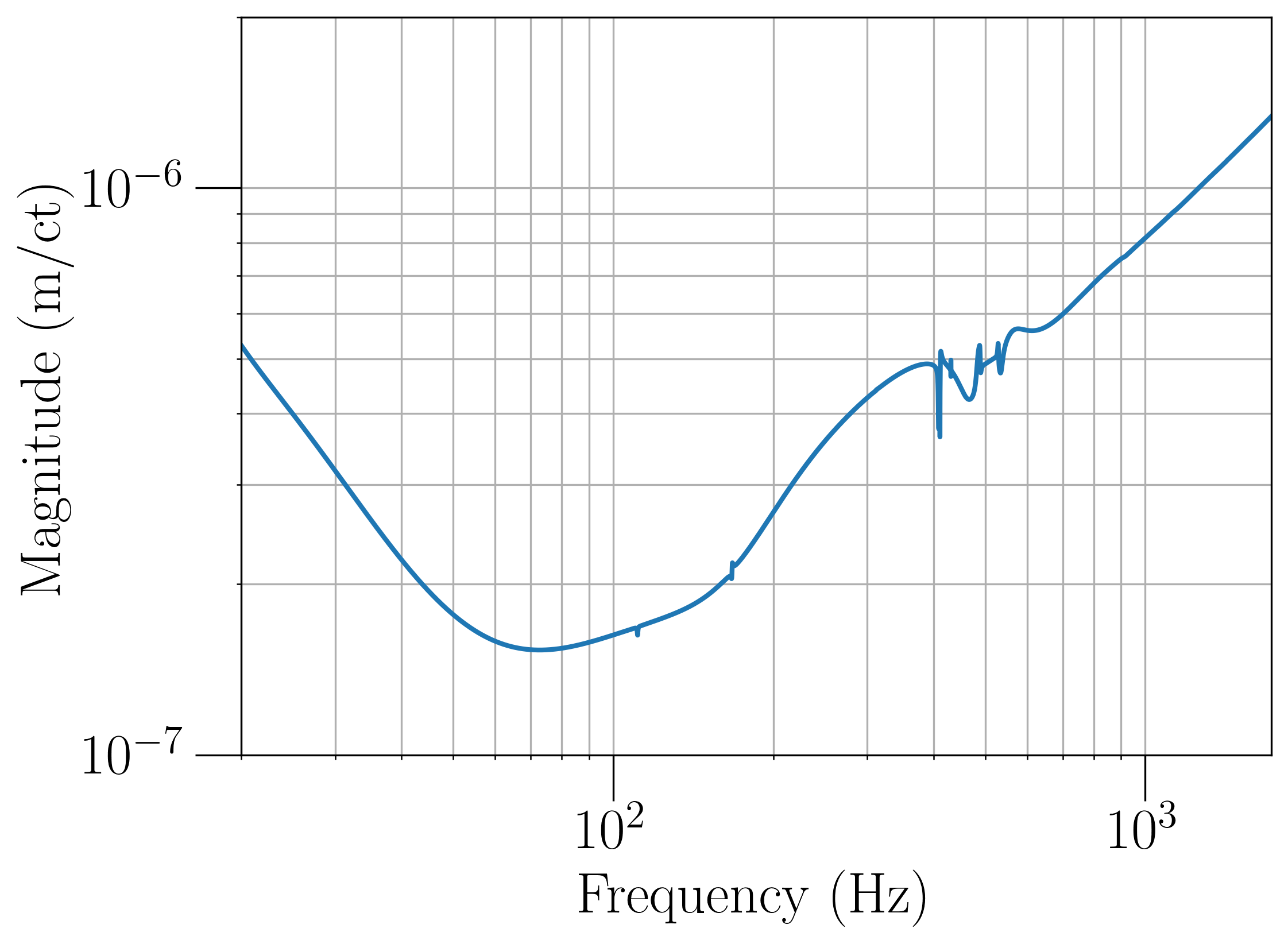
Apart from the notch filters used to prevent the excitation of resonances of the test mass suspensions, is a smooth function of frequency that is decided by the feedback control morphology used. The total response function, as shown in Eq. 9, is a function of , , and . Fig. 3 shows the response function we use in our analysis.
IV Analysis Method
In this work, we look at the effects of calibration uncertainties on the recovery of GWB and on the parameter estimation of the recovered GWB. Specifically, we look at the isotropic GWBs described by power-law models with power-law indices of (see Sec. II).
If the response function used to calibrate the digitized signal in Eq. 8 is not the true response function, then we get,
| (12) | |||||
| (13) |
where true and calc correspond to the true and calculated quantities respectively. In the above Eq. 12, we have defined as,
| (14) |
for convenience. The uncertainties in the calibration process enter the GW analyses as shown above. We note here that , with measurement uncertainty, can be calculated using a length (or frequency) reference such as a photon calibrator Clubley et al. 2001; Mossavi et al. 2006; Accadia et al. 2014; Goetz et al. 2009; Karki et al. 2016, but due to difficulty in the implementation is traditionally used in the calibration process leading to the difference we see in the Eq.12. The is usually in a non-parametric form while is parameterized with a relatively small number of parameters (Eq. 9). Hence from an implementation point of view, is more convenient. Because of the simple parameterization, changes in can also be easily tracked, which is also important for calibration. Moreover, the ratios are usually very close to one, and hence use of is well justified.
Due to the measurement uncertainties in , the estimation of the ratios has both systematic and statistical uncertainties associated with it. Using Eq. 12 in Eqs.4 and 6 we get,
| (15) |
and
| (16) |
The Eqs. 15 and 16 provide a way to estimate the effects of calibration uncertainties on the signal estimate and its variance . If we further assume that the ratios are real, i.e., the difference is only in the magnitude, then we get,
| (17) | |||||
| (18) |
where nocal subscript corresponds to the quantities calculated in the absence of calibration uncertainties that we want. With this assumption, the simulation becomes a little bit easier. We can start with and calculated from the simulated data and using Eqs. 17, 18 and 7 we can estimate the effects of calibration uncertainties on the calculation of and . However, in Sec.V we also show the results without using this assumption. Since the response functions, themselves are functions of (Eq. 11), (Eq. 10) and the number of free parameters in the above equations becomes large. Due to the large number of parameters, it is difficult to calculate the effects analytically, so we use numerical simulation to calculate the effects. This method becomes more valuable when including a more complicated signal model and additional calibration parameters.
For the results reported in this paper, we use one week of simulated data for Hanford and Livingston detectors using advanced LIGO design sensitivity Abbott et al. 2020. Here, one week of data is chosen to represent the traditional long-duration analyses of GWB and to avoid complexities arising from large SNRs in individual segments Allen and Romano 1999. We use publicly available LVK code packages sto to calculate and . We use standard search parameters of 192-sec segment duration and frequencies from 20 Hz to 1726 Hz with a frequency resolution of 1/32 Hz as used in the LVK isotropic GWB searches Abbott et al. 2017; Abbott et al. 2019b; Abbott et al. 2021d. In this work, we use the same calibration model for Hanford and Livingston detectors described in Sec. III.
We do the following to calculate the effects of calibration uncertainties on the recovery of GWB signal. As indicated in the Eqs. 17 and 18, we multiply the and estimators of each segment calculated using LVK code packages by distributions representing the ratios . We assume Gaussian distributions for , centered at one with standard deviations defined by the desired calibration uncertainty. We also truncate the Gaussian distribution at 2-sigma points on both sides to avoid the realization of unrealistic values for (for example, values close to zero or even negative). Then, using Eqs. 7, we combine the segment-wise and frequency-dependent results of to get the final estimate and its uncertainty. Then we use SNR, defined in a frequentist approach Matas and Romano 2021, given by,
as the detection statistics in the search for an isotropic GWB. We then compare these results against the results obtained without any calibration uncertainties. Since the difference between these results is just the application of calibration uncertainties, the differences would typically show the effects of calibration uncertainties on and .
V results
In this section, we present the results of our studies. To generate these results, we initially assume that the ratios of response function are real and hence use Eqs. 17 and 18. We note that this assumption is used to marginalize calibration uncertainties in the LVK isotropic GWB analyses Abbott et al. 2017; Abbott et al. 2019b; Abbott et al. 2021d. However, for comparison, we also produce results by additionally using 1-sigma phase uncertainties of , the maximum of what was seen in LIGO detectors during the observing run O3 Sun et al. 2020. This is to show how much phase uncertainties that are currently not included in the GWB analyses affect the final results. At each frequency, we model the magnitude of by a Gaussian distribution with a mean one and standard deviation that is small compared to one and phase of by a Gaussian distribution with a mean zero and standard deviation of . As indicated earlier, we also truncate the Gaussian distribution at 2-sigma values to avoid unrealistic realizations of .
V.1 Effect of calibration uncertainties on the isotropic GWB detection
The recovered values of the , and SNR at various levels of calibration uncertainties for the three power law models are shown in Fig. 4. In this analysis, we increase the uncertainty from to in steps of . We also repeat the analysis times, regenerating the values times at each uncertainty level to calculate the spread on the recovered values. We also compare the results, including 1-sigma phase uncertainties of .
 |
 |
 |
 |
 |
 |
 |
 |
 |
From the plots, we see that as we increase the values of uncertainties, there are changes in the recovered values of , , and SNR. The recovered values are underestimated, and the trends are similar for the three values. However, the changes in the recovered SNRs are small, almost negligible, below the calibration uncertainties of . Since SNR is generally used as a detection statistic, this suggests that the detection of an isotropic GWB is not significantly affected by the uncertainties in the calibration. We also see a slight reduction in the SNR for larger calibration uncertainties. The SNR dependence on the calibration uncertainty goes as where is the standard deviation of the Gaussian distribution used for the different realizations of . This quadratic dependence agrees with the results previously reported in the literature Allen 1996.
The , change by when we change the uncertainty of response function by . The reduction in the estimated can be attributed to how we combine different time segments and frequency bins. Since we use weighted average method (see Eq. 7), any downward fluctuations in individual due to calibration uncertainties will bring down the final . A similar effect could be attributed to the reduction in the final . This suggests that the recovered values of and are biased in the presence of calibration uncertainties. Since the upper limits on , for example, 95 % upper limit in the frequentist approach, can be written as
calibration uncertainties are also expected to bias the upper limit calculations. From our results, we see that if the calibration (magnitude) uncertainty is , the upper limit would be underestimated by . Since this dependence on the calibration uncertainty is quadratic, this effect could become significant at larger calibration uncertainties. Such biases are not completely taken into account when estimating or while calculating upper limits on in the analyses reported in the literature Abbott et al. 2017; Abbott et al. 2019b; Abbott et al. 2021d and need to be accounted for in future analyses. The plots also suggest that including phase uncertainties at the level of does not change the results significantly. Hence, as done in LVK analyses Abbott et al. 2017; Abbott et al. 2019b; Abbott et al. 2021d, phase uncertainties can be neglected if they are when searching for isotropic GWB using LVK data.
V.2 Effects of the calibration uncertainties on the parameter estimation of isotropic GWBs
The second part of the study looks at the effects of calibration uncertainties on estimating the parameters of the isotropic GWB signals. Here we mainly focus on the estimation of and (see Eq. 3). In Sec. V.1, Fig. 4 already shows the effect of the uncertainties of the response function as a whole on the recovery of . Instead of the uncertainties of the total response function, in this section, we look at the effects of individual calibration parameters on the recoveries of and . Since we are using the parameters that make up the calibration model, in the literature, this is considered a physically motivated approach to include calibration uncertainties in the signal analyses Payne et al. 2020; Vitale et al. 2021. In this study we mainly focus on the parameters , (see Sec. III.1), , and (see Sec. III.2). Other parameters in the response function tend to be more or less constant during an observing run, or their effects are small, and hence we do not include them here.
The maximum likelihood values of the recovered parameters and , for , as functions of errors on the various calibration parameters are shown in Fig. 5.
 |
 |
 |
 |
 |
 |
The plots in Fig. 5 show the recovered values of and as we increase the errors on the calibration parameters , , , and in the response function used to calibrate the detector output. For testing the recovery, we inject isotropic GWBs with amplitudes of for respectively and try to recover them with and without errors on the above calibration parameters. On the right side of the plots in Fig. 5, we also show the difference between the injected and recovered values normalized by the 1-sigma uncertainties in the recovery. To have a common y-axis on the right side, for each , we use the largest 1-sigma uncertainty we observe among different calibration parameters for the normalization.
We use the maximum likelihood method described in Mandic et al. 2012 and use dynesty Speagle 2020 sampler in bilby Ashton et al. 2019 package for sampling the likelihoods and estimating the maximum likelihood values of and (shown in Fig. 5) from and . From the plots in Fig. 5, we see that when the errors on the calibration model parameters are zero, we recover the injected values very well. However, the recovered values of and become biased as we increase the error on the calibration model parameters. The errors on , and significantly bias the recoveries of and while and have very little effect. For example, for , with error on the the recovered is away from its true value, while with error on the the recovered is away from its true value. We also notice that, even though significantly affects the estimate, it has minimal impact on the recovery of . These effects are likely due to how these different terms contribute to the interferometer response function. Rewriting Eq. 9 into contributions from different components, we get,
| (19) | |||||
Fig. 6 shows the relative contribution of the different terms in Eq. 19 to the response function and also 90 % search sensitivity region for the isotropic GWB. The 90 % isotropic GWB search sensitivity region increases as we increase the values of . For , the 90 % search sensitivity region extends up to Hz, while for and , the 90 % search sensitivity regions extend up to Hz and Hz respectively.
We see that in the 90 % sensitivity region, penultimate and test mass actuation and sensing functions make the most significant contributions. The top test mass actuation function contributes to the response function in the Hz band and hence does not affect the signal recovery. In the sensing function (see Eq.10), the dominant contribution comes from . Since the typical value of of advanced LIGO detectors during the O3 run was and the 90 % search sensitivity region extents only up to a maximum of Hz (for ), the effect of on the estimation of the parameters is minimal.
Since the values of 0 and 2/3 are relatively closer, the results of and in Fig. 5 are very similar. We also observe that the result for is slightly different. Since probes a much larger frequency band of Hz where contributions from and to the response function tend to be larger on average compared to the other parameters (see Fig. 6), and start to affect the recoveries of and significantly. We see this for in Fig. 5.
The design of the detector, for example, the finesse of arm and recycling cavities, determines the cavity pole frequency, while the control architecture of the detector determines the relative contributions of different actuation stages. Thus, the effects of different calibration factors on the isotropic GWB search heavily depend on the detector’s design and operation.

We also try to simultaneously estimate the calibration and GWB signal parameters to see how well we can do. Here we use (simulated) uncalibrated raw digital signals to extract all the parameters. Fig. 7 shows an example of the simultaneous estimation of all the parameters for the signal model. The plot shows that, along with the GWB model parameters, we can also infer the values , , and to some level, but recoveries of and are poor which are consistent with the results in Fig. 5. For comparison, we also show the recovery of GWB model parameters using calibrated data without any uncertainties. The plots also have the Bayes factors, comparing the signal vs. noise hypothesis for those two cases. We see that the Bayes factors do not change significantly in the two cases (as expected, it is slightly lower when we estimate calibration parameters also). However, the posteriors of GWB parameters are very broad and probably biased when we simultaneously estimate the GWB and calibration model parameters. So it is crucial to have well-calibrated data to get better posteriors on the signal parameters and a better Bayes factor.

VI Conclusions
In this work, we have studied the effect of calibration uncertainties on the detection and parameter estimation of isotropic GWB signals. We focused on the amplitude () and power law index () of power-law isotropic GWBs. We find that, for the second generation of gravitational wave detectors, when the calibration uncertainties are less than , they do not significantly affect the detection of a GWB signal. The calibration uncertainties of the LIGO detectors reported during the last observing run O3 are well within this limit Sun et al. 2020.
We also find that the recovery of isotropic GWB model parameters could be affected depending on which calibration parameter is poorly constrained and its uncertainty level. The recovered values of signal parameters are biased due to errors in calibration model parameters. Even though the current errors on the individual model parameters of LIGO detectors are much smaller (), the cumulative effect of the different parameters could bias the recovered GWB parameters. Currently, this bias is not considered during the GWB parameter estimation or upper limit calculation. For a calibration uncertainty of % of the interferometer response function (90 % maximum reported for the LIGO detectors during O3), the biases in estimating GWB amplitudes or its upper limits are not significant %. However, this might become significant for larger calibration uncertainties, especially when we try to differentiate between different models of GWB. In this work, we also try to estimate the isotropic GWB and calibration model parameters simultaneously and find that we could detect the GWB signal, albeit with some loss of Bayes factor (SNR). However, the posteriors of the GWB signal parameters become very broad and probably biased due to their correlation with some of the calibration parameters. This suggests the importance of well-calibrated data for detecting and recovering GWB signals, which is expected to be in the near future.
We also note that the analysis presented in this paper highly depends on the GW detectors’ calibration model (parameters). Hence, one might need to repeat this study when the calibration model changes significantly, for example, for future detectors. However, if the calibration uncertainties are kept small (), as we see in our analysis in this paper, the effects on the isotropic GWB analyses are expected to be small. Since the calibration model depends on the detector design and its control system architecture, one could also choose to design future detectors that would reduce the effect of calibration uncertainties. This is something that could be studied further. One could also extend the study reported in this paper to estimate the effect of calibration uncertainties on the GWB with more complicated model parameters or anisotropic GWB.
Acknowledgements
The authors thank Jeffrey S Kissel for providing useful comments on the draft. The authors acknowledge the use of the IUCAA LDG cluster Sarathi for the computational/numerical work. J. Yousuf also acknowledges IUCAA for providing accommodation while carrying out this work. J. Yousuf is thankful to the Department of Science and Technology (DST), Government of India, for providing financial assistance through INSPIRE Fellowship. For this work, we used the software packages pyDARM pyd, bilby Ashton et al. 2019, stochastic sto and Matplotlib Hunter 2007.
References
- Abbott et al. (2016a) B. P. Abbott et al. (LIGO Scientific Collaboration and Virgo Collaboration), Phys. Rev. Lett. 116, 061102 (2016a).
- Aasi et al. (2015a) J. Aasi et al. (LIGO Scientific Collaboration), Class. Quant. Grav. 32, 074001 (2015a).
- Acernese et al. (2015) F. Acernese et al. (VIRGO), Class. Quant. Grav. 32, 024001 (2015), arXiv:1408.3978 [gr-qc] .
- Abbott et al. (2019a) B. P. Abbott et al. (LIGO Scientific Collaboration and Virgo Collaboration), Phys. Rev. X 9, 031040 (2019a).
- Abbott et al. (2021a) R. Abbott et al. (LIGO Scientific Collaboration and Virgo Collaboration), Phys. Rev. X 11, 021053 (2021a).
- Abbott et al. (2021b) R. Abbott et al. (LIGO Scientific Collaboration and Virgo Collaboration and KAGRA Collaboration), (2021b), https://doi.org/10.48550/arXiv.2111.03606, arXiv:2111.03606 [gr-qc] .
- Abbott et al. (2016b) B. P. Abbott et al. (LIGO Scientific Collaboration and Virgo Collaboration), Phys. Rev. Lett. 116, 131102 (2016b).
- Abbott et al. (2018) B. P. Abbott et al. (LIGO Scientific Collaboration and Virgo Collaboration), Phys. Rev. Lett. 120, 091101 (2018), arXiv:1710.05837 [gr-qc] .
- Abbott et al. (2021c) R. Abbott et al. (LIGO Scientific Collaboration and Virgo Collaboration and KAGRA Collaboration), (2021c), 10.48550/ARXIV.2111.03634.
- Regimbau (2022) T. Regimbau, Symmetry 14 (2022), 10.3390/sym14020270.
- Buonanno et al. (2005) A. Buonanno, G. Sigl, G. G. Raffelt, H.-T. Janka, and E. Müller, Phys. Rev. D 72, 084001 (2005).
- Howell et al. (2004) E. Howell, D. Coward, R. Burman, D. Blair, and J. Gilmore, Mon. Not. Roy. Astron. Soc. 351, 1237 (2004).
- Rosado (2012) P. A. Rosado, Phys. Rev. D 86, 104007 (2012).
- Zhu et al. (2011) X.-J. Zhu, X.-L. Fan, and Z.-H. Zhu, Astrophys. J. 729, 59 (2011).
- Caprini and Figueroa (2018) C. Caprini and D. G. Figueroa, Classical and Quantum Gravity 35, 163001 (2018).
- Regimbau (2011) T. Regimbau, Research in Astronomy and Astrophysics 11, 369 (2011).
- de Freitas Pacheco (2020) J. A. de Freitas Pacheco, arXiv e-prints , arXiv:2001.09663 (2020), arXiv:2001.09663 [astro-ph.HE] .
- Romano and Cornish (2017) J. D. Romano and N. J. Cornish, Living Reviews in Relativity 20, 2 (2017), arXiv:1608.06889 [gr-qc] .
- Maggiore (2000) M. Maggiore, Phys. Rep. 331, 283 (2000), arXiv:gr-qc/9909001 [gr-qc] .
- Abbott et al. (2021d) B. Abbott et al. (LIGO Scientific Collaboration, Virgo Collaboration, and KAGRA Collaboration), Phys. Rev. D 104, 022004 (2021d).
- Abbott et al. (2021e) B. Abbott et al. (LIGO Scientific Collaboration, Virgo Collaboration, and KAGRA Collaboration), Phys. Rev. D 104, 022005 (2021e).
- Abbott et al. (2020) B. Abbott et al. (KAGRA Collabration, LIGO Scientific Collaboration, and VIRGO Collaboration), Living Rev. Rel. 23, 3 (2020), arXiv:1304.0670 [gr-qc] .
- Reitze et al. (2019) D. Reitze et al., Bulletin of the AAS 51 (2019), https://baas.aas.org/pub/2020n7i035.
- Punturo et al. (2010) M. Punturo et al., Classical and Quantum Gravity 27, 194002 (2010).
- Périgois et al. (2021) C. Périgois, C. Belczynski, T. Bulik, and T. Regimbau, Phys. Rev. D 103, 043002 (2021).
- Regimbau et al. (2017) T. Regimbau, M. Evans, N. Christensen, E. Katsavounidis, B. Sathyaprakash, and S. Vitale, Phys. Rev. Lett. 118, 151105 (2017).
- Allen and Romano (1999) B. Allen and J. D. Romano, Phys. Rev. D 59, 102001 (1999).
- Abbott et al. (2017) B. P. Abbott et al. (LIGO Scientific Collaboration and Virgo Collaboration), Phys. Rev. Lett. 118, 121101 (2017).
- Abbott et al. (2019b) B. Abbott et al. (LIGO Scientific Collaboration, Virgo Collaboration), Phys. Rev. D 100, 061101 (2019b), arXiv:1903.02886 [gr-qc] .
- Whelan et al. (2014) J. T. Whelan, E. L. Robinson, J. D. Romano, and E. H. Thrane, Journal of Physics: Conference Series 484, 012027 (2014).
- Allen (1996) B. Allen, LIGO Techn. Report: LIGO-T960189 (1996).
- Vitale et al. (2012) S. Vitale, W. Del Pozzo, T. G. F. Li, C. Van Den Broeck, I. Mandel, B. Aylott, and J. Veitch, Phys. Rev. D 85, 064034 (2012).
- Farr et al. (2014) W. Farr, B. Farr, and T. Littenberg, LIGO Techn. Report: LIGO-T1400682 (2014).
- Hall et al. (2019) E. D. Hall, C. Cahillane, K. Izumi, R. J. E. Smith, and R. X. Adhikari, Classical and Quantum Gravity 36, 205006 (2019).
- Payne et al. (2020) E. Payne, C. Talbot, P. D. Lasky, E. Thrane, and J. S. Kissel, Phys. Rev. D 102, 122004 (2020).
- Vitale et al. (2021) S. Vitale, C.-J. Haster, L. Sun, B. Farr, E. Goetz, J. Kissel, and C. Cahillane, Phys. Rev. D 103, 063016 (2021).
- Essick (2022) R. Essick, Phys. Rev. D 105, 082002 (2022).
- Ade et al. (2016) P. A. R. Ade et al., Astron. Astrophys. 594, A13 (2016).
- Sandick et al. (2006) P. Sandick, K. A. Olive, F. Daigne, and E. Vangioni, Phys. Rev. D 73, 104024 (2006).
- Aasi et al. (2015b) J. Aasi et al. (LIGO Scientific Collaboration and Virgo Collaboration), Phys. Rev. D 91, 022003 (2015b).
- Akutsu et al. (2021a) T. Akutsu et al., Progress of Theoretical and Experimental Physics 2021 (2021a), 10.1093/ptep/ptab018, 05A102, https://academic.oup.com/ptep/article-pdf/2021/5/05A102/38109702/ptab018.pdf .
- Abbott et al. (2017) B. P. Abbott et al. (LIGO Scientific Collaboration), Phys. Rev. D 95, 062003 (2017).
- Sun et al. (2020) L. Sun, E. Goetz, J. S. Kissel, J. Betzwieser, S. Karki, A. Viets, M. Wade, D. Bhattacharjee, V. Bossilkov, P. B. Covas, L. E. H. Datrier, R. Gray, S. Kandhasamy, Y. K. Lecoeuche, G. Mendell, T. Mistry, E. Payne, R. L. Savage, A. J. Weinstein, S. Aston, A. Buikema, C. Cahillane, J. C. Driggers, S. E. Dwyer, R. Kumar, and A. Urban, Classical and Quantum Gravity 37, 225008 (2020).
- Viets et al. (2018) A. D. Viets, M. Wade, A. L. Urban, S. Kandhasamy, J. Betzwieser, D. A. Brown, J. Burguet-Castell, C. Cahillane, E. Goetz, K. Izumi, S. Karki, J. S. Kissel, G. Mendell, R. L. Savage, X. Siemens, D. Tuyenbayev, and A. J. Weinstein, Classical and Quantum Gravity 35, 095015 (2018).
- Acernese et al. (2022) F. Acernese et al., Classical and Quantum Gravity 39, 045006 (2022).
- Akutsu et al. (2021b) T. Akutsu et al., Progress of Theoretical and Experimental Physics 2021 (2021b), 10.1093/ptep/ptab018, 05A102.
- Cahillane et al. (2017) C. Cahillane, J. Betzwieser, D. A. Brown, E. Goetz, E. D. Hall, K. Izumi, S. Kandhasamy, S. Karki, J. S. Kissel, G. Mendell, R. L. Savage, D. Tuyenbayev, A. Urban, A. Viets, M. Wade, and A. J. Weinstein, Phys. Rev. D 96, 102001 (2017).
- (48) https://pypi.org/project/pydarm/.
- (49) https://alog.ligo-wa.caltech.edu/aLOG/index.php?callRep=48578.
- (50) https://alog.ligo-la.caltech.edu/aLOG/index.php?callRep=45314.
- Tuyenbayev et al. (2016) D. Tuyenbayev, S. Karki, J. Betzwieser, C. Cahillane, E. Goetz, K. Izumi, S. Kandhasamy, J. S. Kissel, G. Mendell, M. Wade, A. J. Weinstein, and R. L. Savage, Classical and Quantum Gravity 34, 015002 (2016).
- Clubley et al. (2001) D. Clubley, G. Newton, K. Skeldon, and J. Hough, Physics Letters A 283, 85 (2001).
- Mossavi et al. (2006) K. Mossavi, M. Hewitson, S. Hild, F. Seifert, U. Weiland, J. Smith, H. Lück, H. Grote, B. Willke, and K. Danzmann, Physics Letters A 353, 1 (2006).
- Accadia et al. (2014) T. Accadia et al., Classical and Quantum Gravity 31, 165013 (2014).
- Goetz et al. (2009) E. Goetz, P. Kalmus, S. Erickson, R. L. Savage, G. Gonzalez, K. Kawabe, M. Landry, S. Marka, B. O’Reilly, K. Riles, D. Sigg, and P. Willems, Classical and Quantum Gravity 26, 245011 (2009).
- Karki et al. (2016) S. Karki, D. Tuyenbayev, S. Kandhasamy, B. P. Abbott, T. D. Abbott, E. H. Anders, J. Berliner, J. Betzwieser, C. Cahillane, L. Canete, C. Conley, H. P. Daveloza, N. De Lillo, J. R. Gleason, E. Goetz, K. Izumi, J. S. Kissel, G. Mendell, V. Quetschke, M. Rodruck, S. Sachdev, T. Sadecki, P. B. Schwinberg, A. Sottile, M. Wade, A. J. Weinstein, M. West, and R. L. Savage, Review of Scientific Instruments 87, 114503 (2016), https://doi.org/10.1063/1.4967303 .
- (57) https://git.ligo.org/stochastic-public/stochastic/.
- Matas and Romano (2021) A. Matas and J. D. Romano, Phys. Rev. D 103, 062003 (2021).
- Mandic et al. (2012) V. Mandic, E. Thrane, S. Giampanis, and T. Regimbau, Phys. Rev. Lett. 109, 171102 (2012).
- Speagle (2020) J. S. Speagle, Mon. Not. Roy. Astron. Soc. 493, 3132 (2020), arXiv:1904.02180 [astro-ph.IM] .
- Ashton et al. (2019) G. Ashton et al., Astrophys. J. Suppl. 241, 27 (2019), arXiv:1811.02042 [astro-ph.IM] .
- Hunter (2007) J. D. Hunter, Computing in Science & Engineering 9, 90 (2007).