Denoising Convolution Algorithms and Applications
to SAR Signal Processing

Convolution operations are used in different practical applications. They often involve large arrays of data and require optimization with respect to memory and computational cost. While input data are usually available only in a discrete form, the standard realization based on a vector-matrix representation is not often efficient since it leads to using sparse matrices. On the other hand, a tensor decomposition looks very attractive because it might reduce the volume of data very drastically, minimizing the number of zero elements. In addition, arithmetic operations between tensors can be implemented efficiently.

There are different forms of tensor decomposition. The most popular approach is based on the canonical decomposition [12] where a multidimensional array is represented (might be approximate) via a sum of outer products of vectors. For matrices, such decomposition is reduced to skeleton decomposition. However, it is known to be unstable in the cases of multiple tensor dimensions, also referred to as tensor modes. The Tucker decomposition [27] represents a natural stable generalization of the canonical decomposition and can provide a high compression rate. The main drawback of the Tucker decomposition is related to the so-called curse of dimensionality; that is, the algorithm’s complexity grows exponentially with the number of tensor modes. A way to overcome these difficulties is to use the Tensor Train (TT) decomposition, which was originally introduced in [23, 24]. Effectively, the TT decomposition represents a generalization of the classical SVD decomposition to the case of multiple modes. It can also be interpreted as a hierarchical Tucker decomposition [10].

Computing the TT decomposition fully can be very expensive if we use the standard TT-SVD algorithm given, e.g., by Algorithm 1 below. Therefore, many modifications to this algorithm were proposed in the literature to help speed it up. One such improvement was presented in [18], where results comparable to those obtained by the TT-SVD algorithm were produced in a fraction of the time for sparse tensor data. Another algorithm that uses the column space of the unfolding tensors was designed to compute the TT cores in parallel; see [26]. The most popular approach to efficiently compute the TT decomposition is based on using a randomized algorithm; see, e.g., [13, 1, 5].

Maximal compression with the TT decomposition can be reached with matrices whose dimensions are powers of two, as proposed in the so-called Quantized TT (QTT) algorithm [20]. As shown in [15], the convolution realized for multilevel Toeplitz matrices via QTT has a logarithmic complexity with respect to the number of elements in each mode, $N$, and is proportional to the number of modes. It is proven that the result cannot be asymptotically improved. However, this algorithm is improved for finite and practically important $N\sim 10^{4}$ in [25] thanks to the cross-convolution in the Fourier (image) space. The improvement is demonstrated for convolutions with three modes with Newton’s potential. It is to be noted that QTT can also be applied to the Fast Fourier Transform (FTT) to decrease its complexity, as shown in [3]. This super-fast FFT (QTT-FFT) beats the standard FFT for extremely large $N$ such as $N\sim 2^{60}$ for one mode tensors and $N\sim 2^{20}$ for tensors with three modes.

For practical applications, a critical issue is denoising. Real-life data, such as radar signals, are typically contaminated with noise. Denoising is not addressed in the papers we have cited previously. However, TT decomposition itself potentially has the property of denoising, owing to the SVD incorporated in the algorithm [4, 8]. In the current work, we propose and implement the low-rank modifications for the previously developed TT-SVD algorithm of [21]. These modifications speed up the computations. We also demonstrate the denoising capacity of numerical convolutions computed using the QTT decomposition. Specifically, we employ a common model for synthetic aperture radar (SAR) signal processing based on the convolution with a sinc imaging kernel (called the generalized ambiguity function) [6, Chapter 2] and show that when a convolution with this kernel is evaluated in the QTT format, the noise level in the resulting image is substantially reduced compared to that in the original data.

It should be observed that most papers on tensor convolution only consider the run time cost of the convolution after the tensor decomposition has been applied to the objective function and the kernel function and either ignores the cost of the actual tensor decompositions or puts it as a side note. In this paper, we consider every step of computing the convolution using the QTT-FFT algorithm, including the decomposition of the arrays into the QTT format using the TT-SVD algorithm (see Algorithm 1), computation of the QTT-FFT algorithm once in that format, and then extracting the data back after the computation is conducted (Section 5). As the QTT decomposition is computationally expensive, we consider several approaches to speed up the decomposition run time. Without these modifications to the TT-SVD decomposition algorithm, the convolution can take a long to compute and is not a practical approach. We provide more detail in section 7.1.

The methods we use to speed up our TT decompositions are based on truncating SVD ranks in the decomposition algorithm (Algorithm 1) and lead to a significant noise reduction in the data (Section 6). Thus, in Chapter 6, we present algorithms to compute convolutions in a reasonable time while significantly reducing the noise in the data at the same time. Our contribution includes developing and analyzing new approaches to speeding up the tensor train decomposition, see Section 5. In Section 6, we consider the effects of convolutions on removing noise in data. Finally, in Section 7, we show numerical examples and compare our results with other approaches to computing convolutions.

The convolution operation is widely used in different applications in signal processing, data imaging, physics, and probability, to name a few. This operation is a way to combine two signals, usually represented as functions, and produce a third signal with meaningful information. The $D$-dimensional convolution between two functions $f$ and $g$ is defined as

Often to compute the convolution numerically, we assume the support of $f$ and $g$, denoted $\text{\rm supp}(f)$ and $\text{\rm supp}(g)$ respectively, are compact. For simplicity, in this paper, we assume $\text{\rm supp}(f)=\text{\rm supp}(g)=[-L,L]^{D}$ for some $L\in\mathbb{R}$. Next, we discretize the domain $[-L,L]^{D}$ uniformly into $N^{D}$ points such that

where $\Delta x=\frac{2L}{N}$ and $\bm{j}=(j_{1},\ldots,j_{D})$. We then let $\bm{f}$ and $\bm{g}$ be $D$-dimensional arrays such that

for all $\bm{j}$. This leads to the discrete convolution $\bm{I}$ such that

where $\bm{1}=(1,\ldots,1)$ and the sums are over all indices $\bm{i}=(i_{1},\ldots,i_{D})$ that lead to legal subscripts. This Riemann sum approximation (2.2) to the integral (2.1) uses the midpoint rule, thus having $\mathcal{O}(\Delta x^{2})$ accuracy.

To compute this convolution directly takes $\mathcal{O}(N^{2D})$ operations, but it can be reduced to $\mathcal{O}(N^{D}\log(N^{D}))$ by using the fast Fourier transform (FFT) and the discrete convolution theorem. The FFT algorithm is an efficient algorithm used to compute the $D$-dimensional discrete Fourier transforms (DFT) of $\bm{\mathcal{V}}\in\mathbb{R}^{N\times\ldots\times N}$,

where the sum is over the multi-indexed array $\bm{j}$,

and $\omega_{N}=e^{-\frac{2\pi\hat{\imath}}{N}}$, where $\hat{\imath}=\sqrt{-1}$ is the imaginary unit. Similarly, the $D$-dimensional inverse discrete Fourier transform (IDFT), such that

of the array $\hat{\bm{\mathcal{V}}}\in\mathbb{R}^{N\times\ldots\times N}$ is given by

Using the discrete Fourier transform, we can compute the circular convolution $\bm{I}^{c}=(\bm{\mathcal{V}}\circledast\bm{\mathcal{W}})$ defined as

by taking the DFT of $\bm{\mathcal{W}}$ and $\bm{\mathcal{V}}$, multiplying the results together, and then taking the IDFT of the given result. Thus, we have

where $\odot$ is Hadamard product (element-wise product) of $D$-dimensional arrays. The circular convolution is the same as the convolution of two periodic functions (up to a constant scaling), thus to obtain the convolution given in (2.2) (also known as a linear convolution), we need to pad the vectors $\bm{f}$ and $\bm{g}$ with at least $N-1$ zeros in each dimension. For example, given the vectors $\bm{f}^{0},\bm{g}^{0}\in\mathbb{R}^{2N-1}$ with

and $\bm{I}^{c}=(\bm{f}^{0}\circledast\bm{g}^{0})$ as the circular convolution between them, the linear convolution $\bm{I}$ in (2.2) is given by

In this paper, we let $g$ be a predefined kernel, such as the SAR generalized ambiguity function (GAF) (see Section 3 and [6, Chapter 2] for detail) and $f$ be a smooth gradually varying function contaminated with white noise. To compute the convolution, we use the QTT decomposition [16] and the QTT-FFT algorithm [3]. The QTT decomposition is a particular case of the more general TT decomposition (see Section 4 and [21] for detail).

SAR is a coherent remote sensing technology capable of producing two-dimensional images of the Earth’s surface from overhead platforms (airborne or spaceborne). SAR illuminates the chosen area on the surface of the Earth with microwaves (specially modulated pulses) and generates the image by digitally processing the returns (i.e., reflected signals). SAR processing involves the application of the matched filter and summation along the synthetic array, which is a collection of successive locations of the SAR antenna along the flight path. Matched filtering yields the image in the direction normal to the platform flight trajectory or orbit (called cross-track or range), while summation along the array yields the image in the direction parallel to the trajectory or orbit (along-the-track or azimuth).

Mathematically, each of the two signal processing stages can be interpreted as the convolution of the signal received by the SAR antenna with a known function. Equivalently, it can be represented as a convolution of the ground reflectivity function, which is the unknown quantity that SAR aims to reconstruct the imaging kernel or generalized ambiguity function. The advantage of this equivalent representation is that it leads to a very convenient partition: the GAF depends on the imaging system’s characteristics, whereas the target’s properties determine the ground reflectivity function. Moreover, image representation via GAF allows one to see clearly how signal compression (a property that pertains to SAR interrogating waveforms) enables SAR resolution, i.e., the capacity of the sensor to distinguish between closely located targets.

In the simplest possible imaging scenario, when the propagation of radar signals between the antenna and the target is assumed unobstructed, and several additional assumptions also hold; the GAF in either range or azimuthal direction is given by the sinc (or spherical Bessel) function:

where the constant $A$ is determined by normalization, $x$ denotes a given direction, and the quantity $\Delta_{x}$ is the resolution in this direction. From the formula (3.1), we see that the resolution is defined as half-width of the sinc main lobe, i.e., the distance from is central maximum to the first zero. When $x$ is the range direction (cross-track), the resolution $\Delta_{x}$ is inversely proportional to the SAR signal bandwidth, see [6, Section 2.4.4]. When $x$ is the azimuthal direction (along-the-track), the resolution is inversely proportional to the length of the synthetic array, i.e., synthetic aperture, see [6, Section 2.4.3]. Note that lower values of $\Delta_{x}$ correspond to better resolution because SAR can tell between the targets located closer to one another. It can also be shown that as $\Delta_{x}\to 0$ the GAF given by (3.1) converges to the $\delta$-function in the sense of distributions [7, Section 3.3]. In this case, the image, which is a convolution of the ground reflectivity with the GAF, coincides with ground reflectivity. This would be ideal because the image would reconstruct the unknown ground reflectivity exactly. This situation, however, is never realized in practice because having $\Delta_{x}\to 0$ requires either the SAR bandwidth (range direction) or synthetic aperture (azimuthal direction) to become infinitely large, which is not possible.

The literature on SAR imaging is vast. Among the more mathematical sources, we mention the monographs [2], and [6].

Consider the $K$-mode, tensor $\bm{\mathcal{A}}\in\mathbb{C}^{M_{1}\times\ldots\times M_{K}}$ such that

where $M_{k}$ is the size of each mode, and $a(i_{1},\ldots,i_{K})\in\mathbb{C}$ are the elements of the tensor $\bm{\mathcal{A}}$ for all $i_{k}=0,\ldots,M_{k}-1$ and $k=1,\ldots,K$. The tensor train format of $\bm{\mathcal{A}}$ decomposes the tensor into $K$ cores $\bm{\mathcal{A}}^{(k)}\in\mathbb{C}^{r_{k-1}\times M_{k}\times r_{k}}$ such that

where the matrices $\bm{\mathcal{A}}^{(k)}(:,i_{k},:)=\bm{A}^{(k)}_{i_{k}}\in\mathbb{C}^{r_{k-1}\times r_{k}},$ for all $i_{k}=0,\ldots,M_{k}-1$, $k=1,\ldots,K$ (In Matlab notation, $\bm{A}^{(k)}_{i_{k}}=\text{squeeze}(\bm{\mathcal{A}}^{(k)}(:,i_{k},:))$, where squeez() is used to convert the $\mathbb{C}^{r_{k-1}\times 1\times r_{k}}$ tensor into a $\mathbb{C}^{r_{k-1}\times r_{k}}$ matrix). The matrix dimensions $r_{k}$, $k=1,\ldots,K$, are referred to as the TT-ranks of the tensor decomposition, and the $3-$mode tensors $\bm{\mathcal{A}}^{(k)}$ are the TT-cores. Since we are interested in the case when $a(i_{1},\ldots,i_{K})\in\mathbb{C}$, we impose the condition $r_{0}=r_{K}=1$. Let $M=\max_{1\leq k\leq K}M_{k}$ and $r=\max_{1\leq k\leq K-1}r_{k}$, then the the tensor $\bm{\mathcal{A}}$, which has $\mathcal{O}(M^{K})$ elements, can be represented with $\mathcal{O}(MKr^{2})$ elements in the TT format.

We can also represent the TT decomposition as the product of tensor contraction operators. Define the tensor contraction between the tensors $\bm{\mathcal{A}}\in\mathbb{C}^{M_{1}\times\ldots\times M_{K}}$ and $\bm{\mathcal{B}}\in\mathbb{C}^{M_{K}\times\ldots\times M_{\tilde{K}}}$ (note that the first dimension size of $\bm{\mathcal{B}}$ equals the last dimension size of $\bm{\mathcal{A}}$) as $\bm{\mathcal{C}}=\bm{\mathcal{A}}\circ\bm{\mathcal{B}}\in\mathbb{C}^{M_{1}\times\ldots\times M_{K-1}\times M_{K+1}\times\ldots\times M_{\tilde{K}}}$ where

Then the TT format of $\bm{\mathcal{A}}$ can be represented as

Before we show how to find the TT-cores, we first need to define a few properties of tensors. First, let the matrix $\bm{A}^{\{k\}}$ be the $k$-th unfolding of the tensor $\bm{\mathcal{A}}$ such that

Thus, we have that $\bm{A}^{\{k\}}\in\mathbb{C}^{M_{1}M_{2}\ldots M_{k}\times M_{k+1}M_{k+2}\ldots M_{K}}$ which we write as

We denote the process of unfolding a tensor $\bm{\mathcal{A}}$ into a matrix $\bm{A}^{\{k\}}\in\mathbb{C}^{M_{1}M_{2}\ldots M_{k}\times M_{k+1}M_{k+2}\ldots M_{K}}$ as

and folding a matrix into a tensor $\bm{\mathcal{A}}\in\mathbb{C}^{M_{1}\times\ldots\times M_{K}}$ as

(Note this is to be consistent with the Matlab function reshape()).

From [21] it can be shown that there exist a TT-decomposition of $\bm{\mathcal{A}}$ such that

Denote the Frobenius norm of a tensor $\bm{\mathcal{A}}\in\mathbb{C}^{M_{1}\times\ldots\times M_{K}}$ as

and the $\varepsilon_{k}$-rank of the matrix $\bm{A}^{\{k\}}$ as

Given a set $\{\varepsilon_{k}\}_{k=1}^{K}$, we can approximate the tensor $\bm{\mathcal{A}}$ with a tensor $\tilde{\bm{\mathcal{A}}}$ in the TT format such that it has TT- ranks $\tilde{r}_{k}\leq\text{ rank}_{\varepsilon_{k}}(\bm{A}^{\{k\}})$ and

In Algorithm 1, we present the TT-SVD algorithm [21], which computes a TT-decomposition of a tensor $\bm{\mathcal{A}}$ with a prescribed accuracy $\varepsilon$. In Section 5, we present some modifications to this algorithm that relax the prescribed tolerance and allow us to compute an approximate decomposition faster. For a tensor $\bm{\mathcal{A}}\in\mathbb{C}^{M_{1}\times\ldots\times M_{K}}$, define

The TT-decomposition can also be applied to tensors with a small number of modes by using the quantized tensor train decomposition (QTT). For instance, let $\bm{v}\in\mathbb{C}^{2^{K}}$ be a vector ($1$-mode tensor). To apply the QTT-decomposition of $\bm{v}$, we reshape it into the $K$-mode tensor $\bm{\mathcal{V}}\in\mathbb{C}^{2\times\ldots\times 2}$ such that

where

then compute the TT-decomposition of the tensor $\bm{\mathcal{V}}$ (you can think of $i_{K}\ldots i_{1}$ as the binary representation of $i$). Extending the QTT-decomposition to matrices ($2$-mode tensors) $\bm{V}\in\mathbb{C}^{2^{K}\times 2^{K}}$ can be done similarly by reshaping them into $2K$-mode tensors $\bm{\mathcal{V}}\in\mathbb{C}^{2\times\ldots\times 2}$, then computing the TT-decomposition of $\bm{\mathcal{V}}$.

We can approximate the discrete Fourier transform of a vector $\bm{v}\in\mathbb{R}^{2^{K}}$ (or 2D discrete Fourier transform of a matrix $\bm{V}\in\mathbb{R}^{2^{K}\times 2^{K}}$) in the QTT format using what is known as the QTT-FFT approximation algorithm [3]. Let $\hat{\bm{v}}=DFT(\bm{v})$ be the discrete Fourier transform of $\bm{v}$ and let $\bm{\mathcal{V}}$ and $\hat{\bm{\mathcal{V}}}$ be the tensors in the QTT-format that represent the vectors $\bm{v}$ and $\hat{\bm{v}}$ respectively. Given $\bm{\mathcal{V}}$, the QTT- FFT approximation algorithm can approximate $\hat{\bm{\mathcal{V}}}$ with a tensor $\tilde{\bm{\mathcal{V}}}$ such that

for some given tolerance $\varepsilon$. Similarly, we could prescribe some maximum TT-rank, $\hat{R}_{\max}$, for the QTT-FFT algorithm such that $\tilde{r}_{k}\leq\hat{R}_{\max}$ for all TT-ranks of $\tilde{\bm{\mathcal{V}}}$, $\{\tilde{r}_{k}\}_{k=0}^{K}$. The QTT-FFT algorithm can easily be modified to the inverse Fourier transform of a vector (or matrix) in the QTT format, which we denote as the QTT-iFFT algorithm.

In practice, we often need to compute the convolution (2.1), where $f$ is the function of interest and $g$ is a given kernel, but $f$ is not given explicitly. Instead, we are given noisy data

at discrete points $\bm{x}_{\bm{j}}$, ${\bm{j}}=(j_{1},\ldots,j_{D})$. In particular, representing the ground reflectivity function for SAR reconstruction in the form (5.1) helps one model the noise in the received data. We assume that $\xi_{\bm{j}}$ is white noise from a normal distribution with the standard deviation $\sigma$, i.e., $\xi_{\bm{j}}\sim\mathcal{N}(0,\sigma^{2})$.

Since the kernel function $g$ is known, we can discretize it as

for the same $\bm{x}_{\bm{j}}$ values as in (5.1). We assume the $D$-dimensional spatial domain is uniformly discretized into $N^{D}$ points where $N=2^{K-1}-1$, see (2). To compute the discrete convolution (2.2), we propose using the quantized tensor train (QTT) decomposition. To represent the arrays in the QTT format, we pad them with zeros such that the new arrays are $D$-mode tensors in $\mathbb{R}^{2^{K}\times\ldots\times 2^{K}}$. We can relax the condition on the size $N$, but to compute the convolution with an FFT algorithm, we need to zero-pad each dimension with at least $N-1$ extra zeros (see Section 2). Also, for the QTT decomposition, we need each dimension to be of size $2^{K}$ for some $K\in\mathbb{N}$. Let $\bm{\mathcal{F}}_{\xi},\bm{\mathcal{G}}$ be the zero-padded tensors representing $\bm{f}_{\xi}$ and $\bm{g}$ respectively in the QTT format. Here, we assume that the discretization of $f$, $\bm{f}$, has a low, but not exactly known, TT-rank in the QTT-format. This is motivated by the fact that many standard piecewise smooth functions naturally have a low TT-rank, see [22, 9, 16].

To find approximations of these tensors in the TT-format, we modify the original TT-SVD algorithm. This is because with the full TT-SVD algorithm, if the tolerance $\varepsilon$ is small, see equation (4.1), the TT-decomposition has close to full rank. Not only does it take a very long time to compute these decompositions, but most of the noise is still present. However, if $\varepsilon$ is too large, the TT-SVD algorithm loses too much information about the true function $f$. For these reasons, we present slight modifications to the TT-SVD algorithm. They are needed to significantly reduce the computing time, as illustrated by the example in Section 7.1.

We consider three different modifications to the TT-SVD algorithm. These modifications are as follows:

1. (1)

   Set some max rank $R_{\max}$ and truncate the SVD in Algorithm 1 with ranks less than or equal to this threshold. Denote this method as the max rank TT-SVD algorithm.

2. (2)

   Set some max rank $R_{\max}$ and replace the SVD in Algorithm 1 with a randomized SVD (RSVD) given in [11] with max ranks set to $R_{\max}$ (see Appendix A). Denote this method as the max rank TT-RSVD algorithm. Note that for this algorithm, we also need to prescribe an oversampling parameter $p$. We could choose from several randomized SVD algorithms, but due to simplicity and effectiveness, we use the approach described in Appendix A. This algorithm implements the direct SVD.

3. (3)

   Truncate the SVD in Algorithm 1 based on when there is a relative drop in singular values, i.e., if $\frac{\sigma_{k+1}}{\sigma_{k}}<\delta~~(0<\delta<1)$ for a given threshold $\delta$, then truncate the singular values less than $\sigma_{k}$. Denote this method as the SV drop off TT-SVD algorithm.

For the max rank TT-RSVD, if the unfolding matrices $\bm{A}^{\{k\}}\in\mathbb{R}^{m_{k}\times n_{k}}$, where $\min(m_{k},n_{k})\leq R_{\max}+p$, then we revert to the max rank TT-SVD algorithm (without the randomized SVD).

We can modify the QTT-FFT and QTT-iFFT algorithms similarly to our modifications of the TT-SVD algorithms to get a low-rank approximation to the discrete Fourier transform representations of $\bm{\mathcal{F}}_{\xi}$ and $\bm{\mathcal{G}}$. For this, we replace the SVD in the QTT-FFT algorithm (QTT-iFFT) with the truncated SVD algorithms (1)-(3) given above, but with possibly a different max rank which we denote $\hat{R}_{max}$ for (1) and (2), or different threshold $\hat{\delta}$ for (3). For the examples in Section 7, we distinguish between $R_{max}$ and $\hat{R}_{max}$. However, we use the same threshold for $\delta$ in the TT-SVD algorithm and the QTT-FFT algorithm. Thus, we do not distinguish between the two. Note that using the threshold (1) in the QTT-FFT algorithm is not new and is mentioned in [3].

With these above modifications to the TT-SVD algorithm and QTT-FFT (QTT-iFFT) algorithms, we propose the following algorithm (Algorithm 2) to approximate the convolution between the $D$-dimensional arrays $\bm{f}$ and $\bm{g}$. For this algorithm, we denote

• •

  $QFFT_{\hat{R}_{\max}(\hat{\delta})}$: QTT-FFT algorithm with a max rank of ${\hat{R}_{\max}}$ (or threshold $\hat{\delta}$),

• •

  $QiFFT_{\hat{R}_{\max}(\hat{\delta})}$: QTT-iFFT algorithm with a max rank of ${\hat{R}_{\max}}$ (or threshold $\hat{\delta}$).

In Theorem 5.2, we show the asymptotic run time behavior of computing a convolution in one spatial dimension ($D=1$) with the max rank TT-SVD algorithm. First, we prove an auxiliary result about the size of the unfolding matrices for this algorithm; see Lemma 5.1. For Theorem 5.2, we consider the whole process of converting the vector into the QTT-format, computing the convolution, then converting the convolution in the QTT format back into a vector, as is demonstrated in Algorithm 2. For the last step, to convert a tensor in the TT-format back into the standard format, we use the ’full’ algorithm from the Matlab toolbox oseledets/TT-Toolbox. This is given in Algorithm 3. We then reshape this tensor into a vector with a bit of run time.

It is well known that the SVD can remove noise from matrix data, as seen in [4, 14], but little research has been done in denoising with tensor decompositions. In [17] and [19], the Tucker decomposition was used to help remove noise from point cloud data and electron holograms, respectively. In [8], it was shown that the TT-decomposition might have some advantages to denoising as opposed to the Tucker decomposition. This is because a low-rank Tucker matrix guarantees a low TT-rank for the data. However, the converse statement is not always true.

Let $\bm{\mathcal{F}}$ be the low TT-rank tensor representing $\bm{f}$ in the QTT format. Then for some core tensors $\bm{\mathcal{F}}^{(k)}\in\mathbb{R}^{r_{k-1}\times 2\times r_{k}}$ with tensor slices $\bm{\mathcal{F}}^{(k)}(:,i_{k},:)=\bm{f}^{(k)}_{i_{k}}\in\mathbb{R}^{r_{k-1}\times r_{k}}$, $i_{k}=0,1$. Each element of $\bm{\mathcal{F}}$ can be represented in the TT format as

where each $\bm{f}^{(k)}_{i_{k}}$ is a low rank matrix. In practice, it is unlikely the data collected has a low-rank TT decomposition since almost all real radar data has noise due to hardware limitations or other signals interfering with the data. Instead, we have the noisy data $\bm{f}_{\xi}$ whose tensor representation is

where $\bm{\xi}$ is the realization of the random noise in the TT format. The tensor $\bm{\mathcal{F}}_{\xi}$ almost surely has full TT-rank when represented exactly in the QTT format. Ideally, we would like to be able to find an approximate TT decomposition $\tilde{\bm{\mathcal{F}}}$ with TT-cores $\tilde{\bm{\mathcal{F}}}^{(k)}$, $k=1,\ldots,K$, using the noisy data such that $\tilde{\bm{\mathcal{F}}}^{(k)}\approx\bm{\mathcal{F}}^{(k)}$. However, it is hard to guarantee any bound on this. We argue, though, that by using our proposed methods when given the noisy data $\bm{\mathcal{F}}_{\xi}$, we can find a TT decomposition $\tilde{\bm{\mathcal{F}}}$ with low rank such that $\tilde{\bm{\mathcal{F}}}\approx\bm{\mathcal{F}}$.

Consider the first iteration of the for loop of algorithm 1, with $\bm{\mathcal{A}}=\bm{\mathcal{A}}_{0}+\bm{\mathcal{A}}_{\xi}$ as the sum of a smooth tensor ($\bm{\mathcal{A}}_{0}$) and a noisy tensor ($\bm{\mathcal{A}}_{\xi}$). Then, after it is reshaped, we obtain the matrix

where $\bm{A}^{\{1\}}_{0}$ is a low rank matrix and $\bm{A}^{\{1\}}_{\xi}$ is added noise. Let $\bm{A}^{\{1\}}=\bm{U}\bm{\Sigma}\bm{V}^{*}+\bm{E}$ be the truncated SVD of $\bm{A}^{\{1\}}$ and $\bm{A}^{\{1\}}_{0}=\bm{U}_{0}\bm{\Sigma}_{0}\bm{V}_{0}^{*}$ be the SVD of $\bm{A}^{\{1\}}_{0}$. Note that $\bm{U}\bm{\Sigma}\bm{V}^{*}\approx\bm{A}_{0}^{\{1\}}$ does not imply that $\bm{U}\approx\bm{U}_{0}$, and thus the TT-core $\bm{\mathcal{A}}^{(1)}$ is not guaranteed to be approximately equal to $\bm{\mathcal{A}}^{(1)}_{0}$, where $\bm{\mathcal{A}}^{(1)}_{0}$ is the first TT-core of $\bm{\mathcal{A}}_{0}$. However, if we let $\bm{\mathcal{A}}^{2}=\bm{\mathcal{A}}$ on the second iteration of the loop in Algorithm 1 (and similarly for $\bm{\mathcal{A}}_{0}$), we do get that the elements of the tensor contraction $\bm{\mathcal{A}}^{(1)}\circ\bm{\mathcal{A}}^{2}\approx\bm{\mathcal{A}}^{(1)}_{0}\circ\bm{\mathcal{A}}^{2}_{0}$. Similarly, if we can approximate the noise-free component on every iteration of the for loop, we obtain an approximation for the tensor $\bm{\mathcal{A}}_{0}$. While we do not have a theoretical bound on this error, our experiments in Section 7 show that this method works well at removing the noise. Since our method computes multiple SVDs, it can reduce a lot more noise than if we just did a single SVD and can do so without excessive smearing.

This section presents some examples in one and two spatial dimensions. The original code for the TT-decompositions and the QTT-FFT algorithms comes from the Matlab toolbox oseledets/TT-Toolbox. We have modified it accordingly for the max rank TT-SVD, max rank TT-RSVD, and SV drop off TT-SVD algorithm, as discussed in Section 5. For all our examples, we compare the run time and errors of computing the convolution (2.1) using several methods. The error for every example is the $l_{2}$ relative error

where in $D$ spatial dimensions

The reference solution, $\bm{I}_{\text{ref}}$, is the discrete convolution (2.2) computed without any noise. In all of the examples, we compare our methods against computing the convolution with the randomized TT-SVD algorithm from [13], as well as computing the true noisy convolution with FFT. In two space dimensions, we also approximate the convolution using a low matrix rank approximation to the noisy data $\bm{f}_{\xi}$, where the truncated rank is determined by the actual matrix rank of $\bm{f}$.

For all of these examples, we use the normalized sinc imaging kernel that corresponds to the GAF (3.1) truncated to a sufficiently large interval $[-L,L]$:

for $D=1$, and

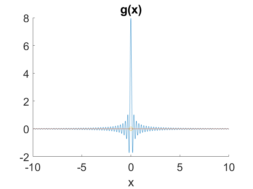
for $D=2$, where the resolution $\Delta_{x}$ in (7.2) and $\Delta_{x}=\Delta_{y}$ in (7.3) is a given parameter. The one- dimensional kernel (7.2) for $\Delta_{x}=0.04\pi$ is shown in Figure 7.1.

In Table 7.1, we present the relative error for each example for $K=20$ when $D=1$, and $K=10$ when $D=2$. In this table, the convolution $\bm{f}_{\xi}*\bm{g}$ is denoted by $\bm{I}_{\xi}$ and computed using the FFT algorithm, the QTT-convolution computed with the max rank TT-SVD algorithm is denoted by $\bm{I}_{QTT_{0}}$, the QTT-convolution computed with the max rank TT-RSVD is denoted by $\bm{I}_{QTT_{r}}$, and the convolution computed using the SV drop off TT-SVD algorithm is denoted by $I_{\delta}$. In turn, the convolutions computed using the randomized TT-decomposition are denoted by $\bm{I}_{RTT}$, and in two dimensions, the convolution computed using low-rank approximations of $\bm{f}$ is denoted by $\bm{I}_{lr}$. For $I_{\delta}$ and $\bm{I}_{lr}$, we also denote what parameter $\delta$ and truncation matrix rank $R$ are used, respectively, for each example using a subscript of the error.

For each example, we show the TT-ranks of the original function without noise, $\bm{f}$, in the QTT format given by the tensor $\bm{\mathcal{F}}$. This QTT approximation is computed with Algorithm 1 with the tolerance $\varepsilon=10^{-10}$. We compute these TT-ranks for $K=20$ when $D=1$ and $K=10$ when $D=2$. However, it is worth noting that these TT-ranks do not change much for any data size. Notice that the max TT-ranks we choose for our algorithms are less than the TT-ranks of $\bm{f}$ from Algorithm 1, yet still provide a reasonable estimate.

References

- [1] Maolin Che and Yimin Wei. Randomized algorithms for the approximations of Tucker and the tensor train decompositions. Adv Comput Math, 45:395–428, 2019.
- [2] Margaret Cheney and Brett Borden. Fundamentals of Radar Imaging, volume 79 of CBMS-NSF Regional Conference Series in Applied Mathematics. SIAM, Philadelphia, 2009.
- [3] Sergey Dolgov, Boris Khoromskij, and Dmitry Savostyanov. Superfast Fourier transform using QTT approximation. J. Fourier Anal. Appl., 18(5):915–953, 2012.
- [4] Brenden P. Epps and Eric M. Krivitzky. Singular value decomposition of noisy data: noise filtering. Experiments in fluids, 60(8):1–23, 2019.
- [5] Krzysztof Fonał and Rafał Zdunek. Distributed and randomized tensor train decomposition for feature extraction. In 2019 International Joint Conference on Neural Networks (IJCNN), pages 1–8, 2019.
- [6] Mikhail Gilman, Erick Smith, and Semyon Tsynkov. Transionospheric synthetic aperture imaging. Applied and Numerical Harmonic Analysis. Birkhäuser/Springer, Cham, Switzerland, 2017.
- [7] Mikhail Gilman and Semyon Tsynkov. A mathematical perspective on radar interferometry. Inverse Problems & Imaging, 16(1):119–152, 2022. doi: 10.3934/ipi.2021043.
- [8] Xiao Gong, Wei Chen, Jie Chen, and Bo Ai. Tensor denoising using low-rank tensor train decomposition. IEEE Signal Processing Letters, 27:1685–1689, 2020.
- [9] Lars Grasedyck. Polynomial approximation in hierarchical tucker format by vector–tensorization. Technical Report 308, Institut für Geometrie und Praktische Mathematik RWTH Aachen, April 2010.
- [10] W. Hackbusch and S. Kühn. A new scheme for the tensor representation. J. Fourier Anal. Appl., 15(5):706–722, 2009.
- [11] N. Halko, P. G. Martinsson, and J. A. Tropp. Finding structure with randomness: probabilistic algorithms for constructing approximate matrix decompositions. SIAM Rev., 53(2):217–288, 2011.
- [12] R.A. Harshman. Foundations of the PARAFAC procedure: Models and conditions for an explanatory multimodal factor analysis. UCLA Working Papers in Phonetics, 16:1–84, December 1970.
- [13] Benjamin Huber, Reinhold Schneider, and Sebastian Wolf. A randomized tensor train singular value decomposition. In Compressed sensing and its applications, Appl. Numer. Harmon. Anal., pages 261–290. Birkhäuser/Springer, Cham, 2017.
- [14] Sunil K. Jha and R. D. S. Yadava. Denoising by singular value decomposition and its application to electronic nose data processing. IEEE Sensors Journal, 11(1):35–44, 2011.
- [15] Vladimir A. Kazeev, Boris N. Khoromskij, and Eugene E. Tyrtyshnikov. Multilevel Toeplitz matrices generated by tensor-structured vectors and convolution with logarithmic complexity. SIAM J. Sci. Comput., 35(3):A1511–A1536, 2013.
- [16] Boris N. Khoromskij. -quantics approximation of - tensors in high-dimensional numerical modeling. Constr. Approx., 34(2):257–280, 2011.
- [17] Jianze Li, Xiao-Ping Zhang, and Tuan Tran. Point cloud denoising based on tensor tucker decomposition. In 2019 IEEE International Conference on Image Processing (ICIP), pages 4375–4379, 2019.
- [18] Lingjie Li, Wenjian Yu, and Kim Batselier. Faster tensor train decomposition for sparse data. Journal of Computational and Applied Mathematics, 405:113972, 2022.
- [19] Yuki Nomura, Kazuo Yamamoto, Satoshi Anada, Tsukasa Hirayama, Emiko Igaki, and Koh Saitoh. Denoising of series electron holograms using tensor decomposition. Microscopy, 70(3):255–264, 09 2020.
- [20] I. V. Oseledets. Approximation of matrices using tensor decomposition. SIAM J. Matrix Anal. Appl., 31(4):2130–2145, 2009/10.
- [21] I. V. Oseledets. Tensor-train decomposition. SIAM Journal on Scientific Computing, 33(5):2295–2317, 2011.
- [22] I. V. Oseledets. Constructive representation of functions in low-rank tensor formats. Constr. Approx., 37(1):1–18, 2013.
- [23] I. V. Oseledets and E. E. Tyrtyshnikov. Breaking the curse of dimensionality, or how to use SVD in many dimensions. SIAM J. Sci. Comput., 31(5):3744–3759, 2009.
- [24] Ivan Oseledets and Eugene Tyrtyshnikov. TT-cross approximation for multidimensional arrays. Linear Algebra Appl., 432(1):70–88, 2010.
- [25] M. V. Rakhuba and I. V. Oseledets. Fast multidimensional convolution in low-rank tensor formats via cross approximation. SIAM J. Sci. Comput., 37(2):A565–A582, 2015.
- [26] Tianyi Shi, Maximilian Ruth, and Alex Townsend. Parallel algorithms for computing the tensor-train decomposition, 2021.
- [27] L.R. Tucker. Some mathematical notes on three-mode factor analysis. Psychometrika, 31:279–311, 1966.