Fairness and Accuracy under Domain Generalization

Machine learning (ML) algorithms trained with real-world data may have inherent bias and exhibit discrimination against certain social groups. To address the unfairness in ML, existing studies have proposed many fairness notions and developed approaches to learning models that satisfy these fairness notions. However, these works are based on an implicit assumption that the data distributions in training and deployment are the same, so that the fair models learned from training data can be deployed to make fair decisions on testing data. Unfortunately, this assumption is commonly violated in real-world applications such as healthcare e.g., it was shown that most US patient data for training ML models are from CA, MA, and NY, with almost no representation from the other 47 states (Kaushal et al. 2020). Because of the distribution shifts between training and deployment, a model that is accurate and fair during training may behave in an unexpected way and induce poor performance during deployment. Therefore, it is critical to account for distribution shifts and learn fair models that are robust to potential changes in deployment environments.

The problem of learning models under distribution shifts has been extensively studied in the literature and is typically referred to as domain adaptation/generalization, where the goal is to learn models on source domain(s) that can be generalized to a different (but related) target domain. Specifically, domain adaptation requires access to (unlabeled) data from the target domain at training time, and the learned model can only be used at a specific target domain. In contrast, domain generalization considers a more general setting when the target domain data are inaccessible during training; instead it assumes there exists a set of source domains based on which the learned model can be generalized to an unseen, novel target domain. For both problems, most studies focus only on the generalization of accuracy across domains without considering fairness, e.g., by theoretically examining the relations between accuracy at target and source domains (Mansour et al. 2008; Mansour et al. 2009; Hoffman et al. 2018; Zhao et al. 2018; Phung et al. 2021; Deshmukh et al. 2019; Muandet et al. 2013; Blanchard et al. 2021; Albuquerque et al. 2019; Ye et al. 2021; Sicilia et al. 2021; Shui et al. 2022) or/and developing practical methods (Albuquerque et al. 2019; Zhao et al. 2020; Li et al. 2018a; Sun & Saenko 2016; Ganin et al. 2016; Ilse et al. 2020; Nguyen et al. 2021). To the best of our knowledge, only Chen et al. 2022; Singh et al. 2021; Coston et al. 2019; Rezaei et al. 2021; Oneto et al. 2019; Madras et al. 2018; Schumann et al. 2019; Yoon et al. 2020 considered the transfer of fairness across domains. However, all of them focused on domain adaptation, and many also imposed rather strong assumptions on distributional shifts (e.g., covariate shifts (Singh et al. 2021; Coston et al. 2019; Rezaei et al. 2021), demographic shift (Giguere et al. 2022), prior probability shift (Biswas & Mukherjee 2021)) that may be violated in practice. Among them, most focused on empirically examining how fairness properties are affected under distributional shifts, whereas theoretical understandings are less studied (Schumann et al. 2019; Yoon et al. 2020). Details and more related works are in Appendix A.

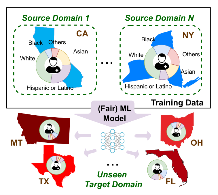
In this paper, we study the transfer of both fairness and accuracy in domain generalization via invariant representation learning, where the data in target domain is unknown and inaccessible during training. A motivating example is shown in Figure 1. Specifically, we first establish a new theoretical framework that develops interpretable bounds on accuracy/fairness at a target domain under domain generalization, and then identify sufficient conditions under which fairness/accuracy can be perfectly transferred to an unseen target domain. Importantly, our theoretical bounds are fundamentally different from the existing bounds, compared to which ours are better connected with practical algorithmic design, i.e., our bounds are aligned with the objective of adversarial learning-based algorithms, a method that is widely used in domain generalization.

Inspired by the theoretical findings, we propose Fairness and Accuracy Transfer by Density Matching (FATDM), a two-stage learning framework such that the representations and fair model learned with source domain data can be well-generalized to an unseen target domain. Last, we conduct the experiments on real-world data; the empirical results show that fair ML models trained with our method still attain a high accuracy and fairness when deployment environments differ from the training. Our main contributions and findings are summarized as follows:

• •

  We consider the transfer of both accuracy and fairness in domain generalization. To the best of our knowledge, this is the first work studying domain generalization with fairness consideration.

• •

  We develop upper bounds for expected loss (Thm. 1) and unfairness (Thm. 3) in target domains. Notably, our bounds are significantly different from the existing bounds as discussed in Appendix A. We also develop a lower bound for expected loss (Thm. 2); it indicates an inherent tradeoff of the existing methods which learn marginal invariant representations for domain generalization.

• •

  We identify sufficient conditions under which fairness and accuracy can be perfectly transferred from source domains to target domains using invariant representation learning (Thm. 4).

• •

  We propose a two-stage training framework (i.e., based on Thm. 5) that learns models in source domains (Sec. 4), which can generalize both accuracy and fairness to target domain.

• •

  We conduct experiments on real-world data to validate the effectiveness of the proposed method.

Notations. Let $\mathcal{X},\mathcal{A}$, and $\mathcal{Y}$ denote the space of features, sensitive attribute (distinguishing different groups, e.g., race/gender), and label, respectively. Let $\mathcal{Z}$ be the representation space induced from $\mathcal{X}$ by representation mapping $g:\mathcal{X}\to\mathcal{Z}$. We use $X$, $A$, $Y$, $Z$ to denote random variables that take values in $\mathcal{X},\mathcal{A},\mathcal{Y},\mathcal{Z}$ and $x,a,y,z$ the realizations. A domain $D$ is specified by distribution $P_{D}:\mathcal{X}\times\mathcal{A}\times\mathcal{Y}\to[0,1]$ and labeling function $f_{D}:\mathcal{X}\to\mathcal{Y}^{\Delta}$, where $\Delta$ is a probability simplex over $\mathcal{Y}$. Similarly, let $h_{D}:\mathcal{Z}\to\mathcal{Y}^{\Delta}$ be a labeling function from representation space for domain $D$. Note that $f_{D},h_{D},g$ are stochastic functions and $f_{D}=h_{D}\circ g$.¹¹ 1 The deterministic labeling function is a special case when it follows Dirac delta distribution in $\Delta$. For simplicity, we use $P_{D}^{V}$ (or $P_{D}^{V|U}$) to denote the induced marginal (or conditional) distributions of variable $V$ (given $U$) in domain $D$.

Error metric. Consider hypothesis $\widehat{f}=\widehat{h}\circ g:\mathcal{X}\to\mathcal{Y}^{\Delta}$, where $\widehat{h}:\mathcal{Z}\to\mathcal{Y}^{\Delta}$ is the hypothesis directly used in representation space. Denote $\widehat{f}(x)_{y}$ as the element on $y$-th dimension which predicts the probability that label $Y=y$ given $X=x$. Then the expected error of $\widehat{f}$ in domain $D$ is defined as $\epsilon^{Acc}_{D}(\widehat{f})=\mathbb{E}_{D}[\mathcal{L}(\widehat{f}(X),Y)]$ for some loss function $\mathcal{L}:\mathcal{Y}^{\Delta}\times\mathcal{Y}\rightarrow\mathbb{R}_{+}$ (e.g., 0-1 loss, cross-entropy loss). Similarly, define the expected error of $\widehat{h}$ in representation space as $\epsilon^{Acc}_{D}(\widehat{h})=\mathbb{E}_{D}[\mathcal{L}(\widehat{h}(Z),Y)]$. Note that most existing works (Albuquerque et al. 2019; Zhao et al. 2018) focus on optimizing $\epsilon^{Acc}_{D}(\widehat{h})$, while our goal is to attain high accuracy in input space, i.e., low $\epsilon^{Acc}_{D}(\widehat{f})$.

Unfairness metric. We focus on group fairness notions (Makhlouf et al. 2021) that require certain statistical measures to be equalized across different groups; many of them can be formulated as (conditional) independence statements between random variables $\widehat{f}(X),A,Y$, e.g., demographic parity ($\widehat{f}(X)\perp A$: the likelihood of a positive outcome is the same across different groups) (Dwork et al. 2012) , equalized odds ($\widehat{f}(X)\perp A|Y$: true positive rate (TPR) and false positive rate (FPR) are the same across different groups), equal opportunity ($\widehat{f}(X)\perp A|Y=1$ when $\mathcal{Y}=\{0,1\}$: TPR is the same across different groups) (Hardt et al. 2016). In the paper, we will present the results under equalized odds (EO) fairness with binary $\mathcal{Y}=\{0,1\}$ and $\mathcal{A}=\{0,1\}$, while all the results (e.g., methods, analysis) can be generalized to multi-class, multi-protected attributes, and other fairness notions. Given hypothesis $\widehat{f}=\widehat{h}\circ g:\mathcal{X}\to\mathcal{Y}^{\Delta}$, the violation of EO in domain $D$ can be measured as $\epsilon^{\texttt{EO}}_{D}(\widehat{f})=\sum_{y\in\mathcal{Y}}\mathcal{D}\Big(P^{\widehat{f}(X)_{1}|Y=y,A=0}_{D}||P^{\widehat{f}(X)_{1}|Y=y,A=1}_{D}\Big)$ for some distance metric $\mathcal{D}(\cdot||\cdot)$.

Problem setup. Consider a problem of domain generalization where a learning algorithm has access to data $\{(x_{k},a_{k},y_{k},d_{k})\}_{k=1}^{m}$ sampled from a set of $N$ source domains $\{D^{S}_{i}\}_{i\in[N]}$, where $d_{k}$ is the domain label and $[N]=\{1,\cdots,N\}$. Our goal is to learn a representation mapping $g:\mathcal{X}\to\mathcal{Z}$ and a fair model $\widehat{h}:\mathcal{Z}\to\mathcal{Y}^{\Delta}$ trained on source domains such that the model $\widehat{f}=\widehat{h}\circ g$ can be generalized to an unseen target domain $D^{T}$ in terms of both accuracy and fairness. Specifically, we investigate under what conditions and by what algorithms we can guarantee that attaining high accuracy and fairness at source domains $\{D^{S}_{i}\}_{i=1}^{N}$ implies small $\epsilon^{\texttt{Acc}}_{D^{T}}(\widehat{f})$ and $\epsilon^{\texttt{EO}}_{D^{T}}(\widehat{f})$ at unknown target domain.

In this section, we present the results on the transfer of accuracy/fairness under domain generalization via domain-invariant learning (proofs are shown in Appendix E). We first examine that for any model $\widehat{h}:\mathcal{Z}\to\mathcal{Y}^{\Delta}$ and any representation mapping $g:\mathcal{X}\to\mathcal{Z}$, how the accuracy/fairness attained at source domains $\{D_{i}^{S}\}_{i=1}^{N}$ can be affected when $\widehat{f}=\widehat{h}\circ g$ is deployed at any target domain $D^{T}$. Specifically, we can bound the error and unfairness at any target domain based on source domains. Before presenting the results, we first introduce the discrepancy measure used for measuring the dissimilarity between domains.

Discrepancy measure. We adopt Jensen-Shannon (JS) distance (Endres & Schindelin 2003) to measure the dissimilarity between two distributions. Formally, JS distance between distributions $P$ and $P^{\prime}$ is defined as

where $\mathcal{D}_{JS}(P||P^{\prime}):=\frac{1}{2}\mathcal{D}_{KL}(P||\frac{P+P^{\prime}}{2})+\frac{1}{2}\mathcal{D}_{KL}(P^{\prime}||\frac{P+P^{\prime}}{2})$ is JS divergence defined based on Kullback–Leibler (KL) divergence $\mathcal{D}_{KL}(\cdot||\cdot)$. Note that unlike KL divergence, JS divergence is symmetric and bounded: $0\leq\mathcal{D}_{JS}(P||P^{\prime})\leq 1$.

While different discrepancy measures such as $\mathcal{H}$ and $\mathcal{H}\Delta\mathcal{H}$ divergences (Ben-David et al. 2010) (i.e., definitions are given in Appendix A) were used in prior works, we particularly consider JS distance because (1) it is aligned with training objective for discriminator in generative adversarial networks (GAN) (Goodfellow et al. 2014), and many existing methods (Ganin et al. 2016; Albuquerque et al. 2019) for invariant representation learning are built based on GAN framework; (2) $\mathcal{H}$ and $\mathcal{H}\Delta\mathcal{H}$ divergences are limited to settings where the labeling functions $f_{D}$ are deterministic (Ben-David et al. 2010; Albuquerque et al. 2019; Zhao et al. 2018). In contrast, our bounds admit the stochastic labeling functions. The limitations of other discrepancy measures and existing bounds are discussed in detail in Appendix A.

The upper bound in Eq. (1) are interpretable and have three terms: term (i) is the averaged error of source domains in input space; term (ii) is the discrepancy between the target domain and the source domains in input space; term (iii) is the discrepancy between the source domains in representation space.³³ 3 In fact, a tighter upper bound for the loss at target domain can be established using strong data processing inequality (Polyanskiy & Wu 2017), as detailed in Appendix D It provides guidance on learning the proper representation mapping $g:\mathcal{X}\to\mathcal{Z}$: to ensure small error at target domain $\epsilon^{\texttt{Acc}}_{D^{T}}(\widehat{f})$, we shall learn representations such that the upper bound of $\epsilon^{\texttt{Acc}}_{D^{T}}(\widehat{f})$ is minimized. Because term (ii) depends on the unknown target domain $D^{T}$ and it’s evaluated in input space $\mathcal{X}\times\mathcal{Y}$, it is fixed and is out of control during training, we can only focus on term (i) and term (iii), i.e., learn representations $Z$ such that errors at source domains $\epsilon^{\texttt{Acc}}_{D^{S}_{i}}(\widehat{f})$ and the discrepancy between source domains in the representation space $d_{JS}(P_{D^{S}_{i}}^{Z,Y},P_{D^{S}_{j}}^{Z,Y})$ are minimized.

Our algorithm in Sec. 4 is designed based on above decomposition: because $P_{D^{S}_{i}}^{Y}$ solely depends on source domain $D^{S}_{i}$, we learn representations by minimizing ${d}_{JS}(P_{D^{S}_{i}}^{Z|Y},P_{D^{S}_{j}}^{Z|Y}),\forall i,j$. Combining Thm. 1 and Corollary 1.1, to ensure high accuracy at unseen target domain $D^{T}$, we learn the representation mapping $g$ and model $\widehat{h}$ such that $P_{D_{i}^{S}}^{Z|Y}$ is invariant across source domains, and meanwhile $\widehat{f}=\widehat{h}\circ g$ attains high accuracy at source domains.

Note that unlike our method, many existing works (Phung et al. 2021; Albuquerque et al. 2019; Ganin et al. 2016) suggest that to ensure high accuracy in domain generalization, representation mapping $g$ should be learned such that $P_{D_{i}^{S}}^{Z}$ is same across domains, i.e., small $d_{JS}(P_{D^{S}_{i}}^{Z},P_{D^{T}}^{Z})$. However, we show that the domain-invariant $P_{D_{i}^{S}}^{Z}$ may adversely increase the error at target domain, as indicated in the Thm. 2 below.

The above lower bound shows an inherent trade-off of approaches that minimize $d_{JS}(P_{D^{S}_{i}}^{Z},P_{D^{T}}^{Z})$ when learning the representations. Specifically, with the domain-invariant $P_{D^{S}_{i}}^{Z}$, the right hand side of Eq. (2) may increase, resulting in an increased error at target domain $\epsilon^{\texttt{Acc}}_{D^{T}}(\widehat{f})$.

Similar to the loss, the unfairness at target domain can also be upper bounded, as presented in Thm. 3.

Similar to Thm. 1, the upper bound in Thm. 3 also has three terms and the second term is out of control during training because it depends on the unseen target domain and is defined in input space. Therefore, to maintain fairness at target domain $D^{T}$, we learn the representation mapping $g$ and model $\widehat{h}$ such that $P_{D_{i}^{S}}^{Z|Y,A}$ is invariant across source domains, and meanwhile $\widehat{f}=\widehat{h}\circ g$ attains high fairness at source domains.

The results above characterize the relations between accuracy/fairness at any target and source domains under any representation mapping $g$ and model $\widehat{h}$. Next, we identify conditions under which the accuracy/fairness attained at sources can be perfectly transferred to a target domain.

Thm. 4 indicates the possibility of attaining the perfect transfer of accuracy/fairness and examples of such representation mappings are provided. Note that these results are consistent with Thm. 1 and Thm. 3, which also suggest learning domain-invariant representations $P_{D_{i}^{S}}^{Z|Y}$ and $P_{D_{i}^{S}}^{Z|Y,A}$.

The accuracy and fairness upper bounds in Sec. 3 shed light on designing robust ML model that can preserve high accuracy and fairness on unseen target domains. Specifically, the model consists of representation mapping $g:\mathcal{X}\rightarrow\mathcal{Z}$ and classifier $\widehat{h}:\mathcal{Z}\rightarrow\mathcal{Y}$ such that (1) the prediction errors and unfairness of $\widehat{f}=\widehat{h}\circ g$ on source domains are minimized; and (2) the discrepancy of learned conditional representations (i.e, $P_{D_{i}^{S}}^{Z|Y}$ and $P_{D_{i}^{S}}^{Z|Y,A}$) among source domains is minimized. That is,

where $\mathcal{L}_{cls}$, $\mathcal{L}_{fair}$, and $\mathcal{L}_{inv}$ are expected losses that penalize incorrect classification, unfairness, and discrepancy among source domains. Hyper-parameters $\omega>0$ and $\gamma>0$ control the accuracy-fairness trade-off and accuracy-invariant representation trade-off, respectively. The usages of these three losses are summarized in Table 1.

Adversarial learning framework (Goodfellow et al. 2014). $\mathcal{L}_{inv}$ in Eq. (3) can be optimized directly with adversarial learning. This is because the training objective of the discriminator in GAN is aligned with our goal of minimizing JS distance between $P_{D_{i}^{S}}^{Z|Y}$ (or $P_{D_{i}^{S}}^{Z|Y,A}$) among source domains, as mentioned in Sec. 3. Specifically, define a set of discriminators $\mathcal{K}=\{k_{y}:y\in\mathcal{Y}\}\cup\{k_{y,a}:y\in\mathcal{Y},a\in\mathcal{A}\}$; each discriminator $k_{y}$ (resp. $k_{y,a}$) aims to distinguish whether a sample with label $y$ (resp. label $y$ and sensitive attribute $a$) comes from a particular domain (i.e., maximize $\mathcal{L}_{inv}$). The representation mapping $g$ should be learned to increase the error of discriminators (i.e., minimize $\mathcal{L}_{inv}$). Therefore, the model and discriminators can be trained simultaneously by playing a two-player minimax game (i.e., $\min_{g}\max_{\mathcal{K}}\mathcal{L}_{inv}(g)$). Combine with the objective of minimizing prediction error and unfairness (i.e., $\min_{g,\widehat{h}}\mathcal{L}_{cls}(g,\widehat{h})+\omega\mathcal{L}_{fair}(g,\widehat{h})$), the overall learning objective is:

However, the above adversarial learning framework for learning domain-invariant representation may not work well when $|\mathcal{Y}\times\mathcal{A}|$ is large: as the label space and sensitive attribute space get larger, the number of discriminators to be learned increases and the training can be highly unstable. A naive solution to tackling this issue is to use one discriminator $\forall y\in\mathcal{Y},a\in\mathcal{A}$. However, this would result in the reduced mutual information between representations and label/sensitive attribute, which may hurt the accuracy. We thus propose another approach to learn the domain-invariant representations.

Proposed solution to learning invariant representations. For any domain $D$, we have:

where $P^{Z|x}$ is domain-independent so we drop $D$ in subscript. Given any two source domains $D^{S}_{i}$ and $D^{S}_{j}$, in general $P_{D^{S}_{i}}^{X|y}\neq P_{D^{S}_{j}}^{X|y}$ and $P_{D^{S}_{i}}^{X|y,a}\neq P_{D^{S}_{j}}^{X|y,a}$ so that it is non-trivial to achieve domain-invariant representations $P_{D^{S}_{i}}^{Z|y}=P_{D^{S}_{j}}^{Z|y}$ and $P_{D^{S}_{i}}^{Z|y,a}=P_{D^{S}_{j}}^{Z|y,a}$. However, if there exist invertible functions $m^{y}_{i,j}:\mathcal{X}\rightarrow\mathcal{X}$ and $m^{y,a}_{i,j}:\mathcal{X}\rightarrow\mathcal{X}$ that can match the density functions of $X$ from $D^{S}_{i}$ to $D^{S}_{j}$ such that $P_{D^{S}_{i}}^{X|y}=P_{D^{S}_{j}}^{m^{y}_{i,j}(X)|y}$ and $P_{D^{S}_{i}}^{X|y,a}=P_{D^{S}_{j}}^{m^{y,a}_{i,j}(X)|y,a}$, and if we can find the representation $Z$ such that $P_{D^{S}_{i}}^{Z|x}=P_{D^{S}_{i}}^{Z|m^{y}_{i,j}(x)}$ and $P_{D^{S}_{i}}^{Z|x}=P_{D^{S}_{i}}^{Z|m^{y,a}_{i,j}(x)}$, then $\forall y\in\mathcal{Y},a\in\mathcal{A}$, we have:

where ${x}^{\prime}=m^{y}_{i,j}(x)$ and ${x}^{\prime\prime}=m^{y,a}_{i,j}(x)$. This observation suggests that to minimize the discrepancy of representation distributions among source domains, we can first find the density mapping functions $m^{y}_{i,j}$ and $m^{y,a}_{i,j}$, $\forall y,a,i,j$, and then minimize the discrepancies between $P^{Z|x},P^{Z|{x}^{\prime}}$, and $P^{Z|{x}^{\prime\prime}}$, $\forall x$. This is formally shown in Thm. 5 below.

Based on Thm. 5, we propose a two-stage learning approach FATDM, as stated below.

Stage 1: learning mapping functions $m^{y}_{i,j}$ and $m^{y,a}_{i,j}$ across source domains. Many approaches can be leveraged to estimate $m^{y}_{i,j}$ and $m^{y,a}_{i,j}$ from data. In our study, we adopt StarGAN (Choi et al. 2018) and CycleGAN (Zhu et al. 2017) as examples; both frameworks are widely used in multi-domain image-to-image translation and can be leveraged. In our algorithm, we independently train two translation models $\textsf{DensityMatch}^{Y}$ and $\textsf{DensityMatch}^{Y,A}$ using StarGAN or CycleGAN, with each used for learning $\{m_{i,j}^{y}\}_{y\in\mathcal{Y},i,j\in[N]}$ and $\{m_{i,j}^{y,a}\}_{y\in\mathcal{Y},a\in\mathcal{A},i,j\in[N]}$, respectively.

Specifically, $\textsf{DensityMatch}^{Y}$ (or $\textsf{DensityMatch}^{Y,A}$) consists of a generator $\mathsf{G}:\mathcal{X}\times[N]\times[N]\to\mathcal{X}$ and a discriminator $\mathsf{D}:\mathcal{X}\to[N]\times\{0,1\}$. The generator takes in real image $x$ and a pair of domain labels $i,j$ as input and generates a fake image; the discriminator aims to predict the domain label of the image generated by the generator and distinguish whether it is fake or real. $\mathsf{G}$ and $\mathsf{D}$ are learned simultaneously by solving the minimax game, and their loss functions are specified in Appendix B. When the training is completed, we obtain two optimal generators from $\textsf{DensityMatch}^{Y}$ and $\textsf{DensityMatch}^{Y,A}$, denoted as $\mathsf{G}^{Y}$ and $\mathsf{G}^{Y,A}$. We shall use $\mathsf{G}^{Y}(\cdot,i,j)$ (resp. $\mathsf{G}^{Y,A}(\cdot,i,j)$) directly as the density mapping function $\{m^{y}_{i,j}(\cdot)\}_{y\in\mathcal{Y}}$ (resp. $\{m^{y,a}_{i,j}(\cdot)\}_{y\in\mathcal{Y},a\in\mathcal{A}}$).

Stage 2: learning domain-invariant representation. Given $\mathsf{G}^{Y}$ and $\mathsf{G}^{Y,A}$ learned in stage 1, we are ready to learn the invariant representation $Z$ by finding $g:\mathcal{X}\to\mathcal{Z}$ such that $g:=\mathcal{N}(\mu(x),\;\sigma^{2}I_{d})$ and minimizes the following:

where $d,{d}^{\prime},{d}^{\prime\prime}$ are domain labels sampled from source domains, $X$ is features sampled from domain $d$, ${X}^{\prime}=\mathsf{G}^{Y}(X,d,{d}^{\prime})$, ${X}^{\prime\prime}=\mathsf{G}^{Y,A}(X,d,{d}^{\prime\prime})$, $\mathcal{L}_{mse}$ is mean squared error. The pseudo-code of our proposed model (FATDM) is in Algorithm 1. The detailed architecture of FATDM is in Appendix B.

We conduct experiments on MIMIC-CXR database (Johnson et al. 2019), which includes 377,110 chest X-ray images associated with 227,827 imaging studies about 14 diseases performed at the Beth Israel Deaconess Medical Center. Importantly, these images are linked with MIMIC-IV database (Johnson et al. 2021) which includes patients’ information such as age, and race; these can serve as sensitive attributes for measuring the unfairness. Based on MIMIC-CXR and MIMIC-IV data, we construct two datasets on two diseases:

• •

  Cardiomegaly disease: we first extract all images related to Cardiomegaly disease, and the corresponding labels (i.e., positive/negative) and sensitive attributes (i.e., male/female); then we partition the data into four domain-specific datasets based on age (i.e., $[18,40),[40,60),[60,80),[80,100)$). We consider age as domain label because it captures the real scenario that there are distribution shifts across patients with different ages.

• •

  Edema disease: we extract all images related to Edema disease, and corresponding labels (i.e., positive/negative) and sensitive attributes (i.e., age with ranges $[18,40),[40,60),[60,80),[80,100)$). Unlike Cardiomegaly data, we construct the dataset for each domain by first sampling images from Edema data followed by $\theta$ degree counter-clockwise rotation, where $\theta\in\{0^{\circ},15^{\circ},30^{\circ},45^{\circ},60^{\circ}\}$. We consider rotation degree as domain label to model the scenario where there is rotational misalignment among images collected from different devices.

Next, we focus on Cardiomegaly disease and the results for Edema disease are shown in Appendix C.

Baselines. We compare our method (i.e., FATDM-StarGAN and FATDM-CycleGAN) with existing methods for domain generalization, including empirical risk minimization, domain invariant representation learning, and distributionally robust optimization, as detailed below.

• •

  Empirical risk minimization (ERM): The baseline that considers all source domains as one domain.

• •

  Domain invariant representation learning: Method that aims to achieve the invariant across source domains. We experiment with G2DM (Albuquerque et al. 2019), DANN (Ganin et al. 2016), CDANN (Li et al. 2018c), CORAL (Sun & Saenko 2016), IRM (Arjovsky et al. 2019). These models focus on accuracy transfer by enforcing the invariance of distributions $P_{D^{S}_{i}}^{Z}$ or $P_{D^{S}_{i}}^{Z|Y}$.

• •

  Distributionally robust optimization: Method that learns a model at worst-case distribution to hope it can generalize well on test data. We experiment with GroupDRO (Sagawa et al. 2019) that minimizes the worst-case training loss over a set of pre-defined groups through regularization.

• •

  ATDM: A variant of FATDM-StarGAN that solely focuses on accuracy transfer. That is, we only enforce the invariance of $P_{D^{S}_{i}}^{Z|Y}$ during learning which is similar to Nguyen et al. 2021.

The implementations of these models except G2DM are adapted from DomainBed framework (Gulrajani & Lopez-Paz 2020). For G2DM, we use the author-provided implementation. For all models, we use ResNet18 (He et al. 2016) as the backbone module of representation mapping $g:\mathcal{X}\to\mathcal{Z}$; and fairness constraint $\mathcal{L}_{fair}$ is enforced as a regularization term added to the original objective functions.

Experiment setup. We follow leave-one-out domain setting in which 3 domains are used for training and the remaining domain serves as the unseen target domain and is used for evaluation. Several metrics are considered to measure the unfairness and error of each model in target domain, including:

• •

  Error: cross-entropy loss (CE), misclassification rate (MR), $\overline{\mbox{AUROC}}$ $:=1-$AUROC, $\overline{\mbox{AUPR}}$ $:=1-$AUPR, $\overline{{F_{1}}}:=1-F_{1}$, where AUROC, AUPR, $F_{1}$ are area under receiver operating characteristic curve, area under precision-recall curve, $F_{1}$ score, respectively.

• •

  Unfairness: we consider both equalized odds and equal opportunity fairness notion, and adopt mean distance (MD) and earth mover’s distance (EMD) as distance metric $\mathcal{D}(\cdot||\cdot)$.

Fairness and accuracy on target domains. We first compare our method with baselines in terms of the optimal trade-off (Pareto frontier) between accuracy and fairness on target domains under different metric pairs. Figure 4 shows the error-unfairness curves (as $\omega$ varies from 0 (no fairness constraint) to 10 (strong fairness constraint)), with $\overline{\mbox{AUROC}}$ and MR as error metric, and equalized odds (measured under distance metrics MD and EMD) as fairness notion; the results for other error metrics are similar and shown in Appendix C. Our observations are as follows: (1) As expected, there is a trade-off between fairness and accuracy: for all methods, increasing $\omega$ improves fairness but reduces accuracy. (2) Among all methods, the Pareto frontiers of FATDM-StarGAN and FATDM-CycleGAN are the bottom leftmost, implying that our method attains a better fairness-accuracy trade-off than baselines. (3) Although fairness constraint is imposed during training for all methods, the fairness attained at source domains cannot be well-generalized to the target domain under other methods. These results validate our theorems and show that enforcing the domain-invariant $P_{D^{S}_{i}}^{Z|Y}$ and $P_{D^{S}_{i}}^{Z|Y,A}$ when learning representations ensures the transfer of both accuracy and fairness. It is worth-noting that under this dataset, the domain-invariant $P_{D^{S}_{i}}^{Z|Y}$ (accuracy transfer) does not imply the domain-invariant $P_{D^{S}_{i}}^{Z|Y,A}$ (fairness transfer). This is because domain $D^{S}_{i}$ (i.e., age) is correlated with label $Y$ (i.e., has a disease) and sensitive attribute $A$ (i.e., gender), making the distribution $P_{D^{S}_{i}}^{Y,A}$ different across domains.

Impact of density mapping model. To investigate whether the performance gain of our method is due to the use of any specific density mapping model, we adopt StarGAN and CycleGAN architectures to learn density mapping functions in our method and compare their performances. Figure 4 shows that FATDM-StarGAN and CycleGAN achieve similar fairness-accuracy trade-off at the target domains and both of them outperform the baselines. This result shows that our method is not limited to any specific density mapping model and is broadly applicable to other architectures.

Impact of invariant representation constraints. We also examine the impact of $\mathcal{L}_{inv}$ on the performance of FATDM-StarGAN at target domains, where we vary the hyper-parameter $\gamma\in[0,5e^{2}]$ at different levels of fairness (i.e., fix $\omega=1,5,10$) and examine how the prediction performances (i.e., AUROC, AUPR, accuracy and $F_{1}$) could change. Figure 5 shows that enforcing domain-invariant constraint $\mathcal{L}_{inv}$ helps transfer the performance from source to target domain, and $\gamma$ that attains the highest accuracy at target domain can be different for different levels of fairness. The results also indicate the fairness-accuracy trade-off, i.e., for any $\gamma$, enforcing stronger fairness constraints (large $\omega$) could hurt prediction performances.

In this paper, we theoretically and empirically demonstrate how to achieve fair and accurate predictions in unknown testing environments. To the best of our knowledge, our work provides the first theoretical analysis to understand the efficiency of invariant representation learning in transferring both fairness and accuracy under domain generalization. In particular, we first propose the upper bounds of prediction error and unfairness in terms of JS-distance, then design the two-stage learning method that minimizes these upper bounds by learning domain-invariant representations. Experiments on the real-world clinical data demonstrate the effectiveness of our study.

The original chest X-ray images and the corresponding metadata can be downloaded from PhysioNet (https://physionet.org/content/mimic-cxr-jpg/2.0.0/; https://physionet.org/content/mimiciv/2.0/). Codes for data processing and proposed algorithms are in supplementary materials. Technical details of the proposed algorithms and experimental settings are in Appendix B. Additional experimental results are in Appendix C. Lemmas used in proofs of the theorems in the main paper are in Appendix D. Complete proofs of the theorems in the main paper and the corresponding lemmas are in Appendix E.

This work was funded in part by the National Science Foundation under award number IIS-2145625, by the National Institutes of Health under award number UL1TR002733, and by The Ohio State University President’s Research Excellence Accelerator Grant.

References

- Agarwal et al. (2018) Alekh Agarwal, Alina Beygelzimer, Miroslav Dudík, John Langford, and Hanna Wallach. A reductions approach to fair classification. In International Conference on Machine Learning, pp. 60–69. PMLR, 2018.
- Albuquerque et al. (2019) Isabela Albuquerque, João Monteiro, Mohammad Darvishi, Tiago H Falk, and Ioannis Mitliagkas. Generalizing to unseen domains via distribution matching. arXiv preprint arXiv:1911.00804, 2019.
- Arjovsky et al. (2019) Martin Arjovsky, Léon Bottou, Ishaan Gulrajani, and David Lopez-Paz. Invariant risk minimization. arXiv preprint arXiv:1907.02893, 2019.
- Bechavod et al. (2020) Yahav Bechavod, Christopher Jung, and Steven Z Wu. Metric-free individual fairness in online learning. Advances in neural information processing systems, 33:11214–11225, 2020.
- Ben-David et al. (2010) Shai Ben-David, John Blitzer, Koby Crammer, Alex Kulesza, Fernando Pereira, and Jennifer Wortman Vaughan. A theory of learning from different domains. Machine learning, 79(1):151–175, 2010.
- Biega et al. (2018) Asia J Biega, Krishna P Gummadi, and Gerhard Weikum. Equity of attention: Amortizing individual fairness in rankings. In The 41st international acm sigir conference on research & development in information retrieval, pp. 405–414, 2018.
- Biswas & Mukherjee (2021) Arpita Biswas and Suvam Mukherjee. Ensuring fairness under prior probability shifts. In Proceedings of the 2021 AAAI/ACM Conference on AI, Ethics, and Society, pp. 414–424, 2021.
- Blanchard et al. (2021) Gilles Blanchard, Aniket Anand Deshmukh, Urun Dogan, Gyemin Lee, and Clayton Scott. Domain generalization by marginal transfer learning. Journal of Machine Learning Research, 22:1–55, 2021.
- Carlucci et al. (2019) Fabio M Carlucci, Antonio D’Innocente, Silvia Bucci, Barbara Caputo, and Tatiana Tommasi. Domain generalization by solving jigsaw puzzles. In Proceedings of the IEEE/CVF Conference on Computer Vision and Pattern Recognition, pp. 2229–2238, 2019.
- Chen et al. (2022) Yatong Chen, Reilly Raab, Jialu Wang, and Yang Liu. Fairness transferability subject to bounded distribution shift. arXiv preprint arXiv:2206.00129, 2022.
- Choi et al. (2018) Yunjey Choi, Minje Choi, Munyoung Kim, Jung-Woo Ha, Sunghun Kim, and Jaegul Choo. Stargan: Unified generative adversarial networks for multi-domain image-to-image translation. In Proceedings of the IEEE conference on computer vision and pattern recognition, pp. 8789–8797, 2018.
- Coston et al. (2019) Amanda Coston, Karthikeyan Natesan Ramamurthy, Dennis Wei, Kush R Varshney, Skyler Speakman, Zairah Mustahsan, and Supriyo Chakraborty. Fair transfer learning with missing protected attributes. In Proceedings of the 2019 AAAI/ACM Conference on AI, Ethics, and Society, pp. 91–98, 2019.
- Deshmukh et al. (2019) Aniket Anand Deshmukh, Yunwen Lei, Srinagesh Sharma, Urun Dogan, James W Cutler, and Clayton Scott. A generalization error bound for multi-class domain generalization. arXiv preprint arXiv:1905.10392, 2019.
- Devroye et al. (2018) Luc Devroye, Abbas Mehrabian, and Tommy Reddad. The total variation distance between high-dimensional gaussians. arXiv preprint arXiv:1810.08693, 2018.
- Dwork et al. (2012) Cynthia Dwork, Moritz Hardt, Toniann Pitassi, Omer Reingold, and Richard Zemel. Fairness through awareness. In Proceedings of the 3rd innovations in theoretical computer science conference, pp. 214–226, 2012.
- Endres & Schindelin (2003) D.M. Endres and J.E. Schindelin. A new metric for probability distributions. IEEE Transactions on Information Theory, 49(7):1858–1860, 2003. doi: 10.1109/TIT.2003.813506.
- Ganin & Lempitsky (2015) Yaroslav Ganin and Victor Lempitsky. Unsupervised domain adaptation by backpropagation. In International conference on machine learning, pp. 1180–1189. PMLR, 2015.
- Ganin et al. (2016) Yaroslav Ganin, Evgeniya Ustinova, Hana Ajakan, Pascal Germain, Hugo Larochelle, François Laviolette, Mario Marchand, and Victor Lempitsky. Domain-adversarial training of neural networks. The journal of machine learning research, 17(1):2096–2030, 2016.
- Giguere et al. (2022) Stephen Giguere, Blossom Metevier, Bruno Castro da Silva, Yuriy Brun, Philip S Thomas, and Scott Niekum. Fairness guarantees under demographic shift. In International Conference on Learning Representations, 2022.
- Goodfellow et al. (2014) Ian Goodfellow, Jean Pouget-Abadie, Mehdi Mirza, Bing Xu, David Warde-Farley, Sherjil Ozair, Aaron Courville, and Yoshua Bengio. Generative adversarial nets. Advances in neural information processing systems, 27, 2014.
- Gulrajani & Lopez-Paz (2020) Ishaan Gulrajani and David Lopez-Paz. In search of lost domain generalization. arXiv preprint arXiv:2007.01434, 2020.
- Gupta & Kamble (2021) Swati Gupta and Vijay Kamble. Individual fairness in hindsight. Journal of Machine Learning Research, 22(144):1–35, 2021.
- Hardt et al. (2016) Moritz Hardt, Eric Price, and Nati Srebro. Equality of opportunity in supervised learning. Advances in neural information processing systems, 29, 2016.
- He et al. (2016) Kaiming He, Xiangyu Zhang, Shaoqing Ren, and Jian Sun. Deep residual learning for image recognition. In Proceedings of the IEEE conference on computer vision and pattern recognition, pp. 770–778, 2016.
- Hoffman et al. (2018) Judy Hoffman, Mehryar Mohri, and Ningshan Zhang. Algorithms and theory for multiple-source adaptation. Advances in Neural Information Processing Systems, 31, 2018.
- Hu et al. (2018) Weihua Hu, Gang Niu, Issei Sato, and Masashi Sugiyama. Does distributionally robust supervised learning give robust classifiers? In International Conference on Machine Learning, pp. 2029–2037. PMLR, 2018.
- Huang et al. (2020) Zeyi Huang, Haohan Wang, Eric P Xing, and Dong Huang. Self-challenging improves cross-domain generalization. In European Conference on Computer Vision, pp. 124–140. Springer, 2020.
- Ilse et al. (2020) Maximilian Ilse, Jakub M Tomczak, Christos Louizos, and Max Welling. Diva: Domain invariant variational autoencoders. In Medical Imaging with Deep Learning, pp. 322–348. PMLR, 2020.
- Jeon et al. (2021) Seogkyu Jeon, Kibeom Hong, Pilhyeon Lee, Jewook Lee, and Hyeran Byun. Feature stylization and domain-aware contrastive learning for domain generalization. In Proceedings of the 29th ACM International Conference on Multimedia, pp. 22–31, 2021.
- Johnson et al. (2021) Alistair Johnson, Lucas Bulgarelli, Tom Pollard, Steven Horng, Leo Anthony Celi, and Mark Roger. Mimic-iv. https://doi.org/10.13026/s6n6-xd98, 2021.
- Johnson et al. (2019) Alistair EW Johnson, Tom J Pollard, Nathaniel R Greenbaum, Matthew P Lungren, Chih-ying Deng, Yifan Peng, Zhiyong Lu, Roger G Mark, Seth J Berkowitz, and Steven Horng. Mimic-cxr-jpg, a large publicly available database of labeled chest radiographs. arXiv preprint arXiv:1901.07042, 2019.
- Kamiran & Calders (2012) Faisal Kamiran and Toon Calders. Data preprocessing techniques for classification without discrimination. Knowledge and information systems, 33(1):1–33, 2012.
- Kaushal et al. (2020) Amit Kaushal, Russ Altman, and Curt Langlotz. Geographic distribution of us cohorts used to train deep learning algorithms. Jama, 324(12):1212–1213, 2020.
- Kim et al. (2021) Daehee Kim, Youngjun Yoo, Seunghyun Park, Jinkyu Kim, and Jaekoo Lee. Selfreg: Self-supervised contrastive regularization for domain generalization. In Proceedings of the IEEE/CVF International Conference on Computer Vision, pp. 9619–9628, 2021.
- Koh et al. (2021) Pang Wei Koh, Shiori Sagawa, Henrik Marklund, Sang Michael Xie, Marvin Zhang, Akshay Balsubramani, Weihua Hu, Michihiro Yasunaga, Richard Lanas Phillips, Irena Gao, et al. Wilds: A benchmark of in-the-wild distribution shifts. In International Conference on Machine Learning, pp. 5637–5664. PMLR, 2021.
- Krueger et al. (2021) David Krueger, Ethan Caballero, Joern-Henrik Jacobsen, Amy Zhang, Jonathan Binas, Dinghuai Zhang, Remi Le Priol, and Aaron Courville. Out-of-distribution generalization via risk extrapolation (rex). In International Conference on Machine Learning, pp. 5815–5826. PMLR, 2021.
- Li et al. (2018a) Haoliang Li, Sinno Jialin Pan, Shiqi Wang, and Alex C Kot. Domain generalization with adversarial feature learning. In Proceedings of the IEEE conference on computer vision and pattern recognition, pp. 5400–5409, 2018a.
- Li et al. (2018b) Ya Li, Mingming Gong, Xinmei Tian, Tongliang Liu, and Dacheng Tao. Domain generalization via conditional invariant representations. In Proceedings of the AAAI conference on artificial intelligence, volume 32, 2018b.
- Li et al. (2018c) Ya Li, Xinmei Tian, Mingming Gong, Yajing Liu, Tongliang Liu, Kun Zhang, and Dacheng Tao. Deep domain generalization via conditional invariant adversarial networks. In Proceedings of the European Conference on Computer Vision (ECCV), pp. 624–639, 2018c.
- Li et al. (2021) Zheren Li, Zhiming Cui, Sheng Wang, Yuji Qi, Xi Ouyang, Qitian Chen, Yuezhi Yang, Zhong Xue, Dinggang Shen, and Jie-Zhi Cheng. Domain generalization for mammography detection via multi-style and multi-view contrastive learning. In International Conference on Medical Image Computing and Computer-Assisted Intervention, pp. 98–108. Springer, 2021.
- Liu et al. (2021) Evan Z Liu, Behzad Haghgoo, Annie S Chen, Aditi Raghunathan, Pang Wei Koh, Shiori Sagawa, Percy Liang, and Chelsea Finn. Just train twice: Improving group robustness without training group information. In International Conference on Machine Learning, pp. 6781–6792. PMLR, 2021.
- Madras et al. (2018) David Madras, Elliot Creager, Toniann Pitassi, and Richard Zemel. Learning adversarially fair and transferable representations. In International Conference on Machine Learning, pp. 3384–3393. PMLR, 2018.
- Makhlouf et al. (2021) Karima Makhlouf, Sami Zhioua, and Catuscia Palamidessi. Machine learning fairness notions: Bridging the gap with real-world applications. Information Processing & Management, 58(5):102642, 2021.
- Mansour et al. (2008) Yishay Mansour, Mehryar Mohri, and Afshin Rostamizadeh. Domain adaptation with multiple sources. Advances in neural information processing systems, 21, 2008.
- Mansour et al. (2009) Yishay Mansour, Mehryar Mohri, and Afshin Rostamizadeh. Multiple source adaptation and the rényi divergence. In Proceedings of the Twenty-Fifth Conference on Uncertainty in Artificial Intelligence, pp. 367–374, 2009.
- Miyato et al. (2018) Takeru Miyato, Toshiki Kataoka, Masanori Koyama, and Yuichi Yoshida. Spectral normalization for generative adversarial networks. arXiv preprint arXiv:1802.05957, 2018.
- Muandet et al. (2013) Krikamol Muandet, David Balduzzi, and Bernhard Schölkopf. Domain generalization via invariant feature representation. In International Conference on Machine Learning, pp. 10–18. PMLR, 2013.
- Nguyen et al. (2021) A Tuan Nguyen, Toan Tran, Yarin Gal, and Atilim Gunes Baydin. Domain invariant representation learning with domain density transformations. Advances in Neural Information Processing Systems, 34, 2021.
- Oneto et al. (2019) Luca Oneto, Michele Donini, Andreas Maurer, and Massimiliano Pontil. Learning fair and transferable representations. arXiv preprint arXiv:1906.10673, 2019.
- Phung et al. (2021) Trung Phung, Trung Le, Tung-Long Vuong, Toan Tran, Anh Tran, Hung Bui, and Dinh Phung. On learning domain-invariant representations for transfer learning with multiple sources. Advances in Neural Information Processing Systems, 34, 2021.
- Polyanskiy & Wu (2014) Yury Polyanskiy and Yihong Wu. Lecture notes on information theory. Lecture Notes for ECE563 (UIUC) and, 6(2012-2016):7, 2014.
- Polyanskiy & Wu (2017) Yury Polyanskiy and Yihong Wu. Strong data-processing inequalities for channels and bayesian networks. In Convexity and Concentration, pp. 211–249. Springer, 2017.
- Qiao et al. (2020) Fengchun Qiao, Long Zhao, and Xi Peng. Learning to learn single domain generalization. In Proceedings of the IEEE/CVF Conference on Computer Vision and Pattern Recognition, pp. 12556–12565, 2020.
- Rame et al. (2021) Alexandre Rame, Corentin Dancette, and Matthieu Cord. Fishr: Invariant gradient variances for out-of-distribution generalization. arXiv preprint arXiv:2109.02934, 2021.
- Rezaei et al. (2021) Ashkan Rezaei, Anqi Liu, Omid Memarrast, and Brian D Ziebart. Robust fairness under covariate shift. In Proceedings of the AAAI Conference on Artificial Intelligence, volume 35, pp. 9419–9427, 2021.
- Sagawa et al. (2019) Shiori Sagawa, Pang Wei Koh, Tatsunori B Hashimoto, and Percy Liang. Distributionally robust neural networks. In International Conference on Learning Representations, 2019.
- Schumann et al. (2019) Candice Schumann, Xuezhi Wang, Alex Beutel, Jilin Chen, Hai Qian, and Ed H Chi. Transfer of machine learning fairness across domains. arXiv preprint arXiv:1906.09688, 2019.
- Shankar et al. (2018) Shiv Shankar, Vihari Piratla, Soumen Chakrabarti, Siddhartha Chaudhuri, Preethi Jyothi, and Sunita Sarawagi. Generalizing across domains via cross-gradient training. In International Conference on Learning Representations, 2018.
- Shi et al. (2021) Yuge Shi, Jeffrey Seely, Philip HS Torr, N Siddharth, Awni Hannun, Nicolas Usunier, and Gabriel Synnaeve. Gradient matching for domain generalization. arXiv preprint arXiv:2104.09937, 2021.
- Shui et al. (2022) Changjian Shui, Boyu Wang, and Christian Gagné. On the benefits of representation regularization in invariance based domain generalization. Machine Learning, pp. 1–21, 2022.
- Sicilia et al. (2021) Anthony Sicilia, Xingchen Zhao, and Seong Jae Hwang. Domain adversarial neural networks for domain generalization: When it works and how to improve. arXiv preprint arXiv:2102.03924, 2021.
- Singh et al. (2021) Harvineet Singh, Rina Singh, Vishwali Mhasawade, and Rumi Chunara. Fairness violations and mitigation under covariate shift. In Proceedings of the 2021 ACM Conference on Fairness, Accountability, and Transparency, pp. 3–13, 2021.
- Sun & Saenko (2016) Baochen Sun and Kate Saenko. Deep coral: Correlation alignment for deep domain adaptation. In European conference on computer vision, pp. 443–450. Springer, 2016.
- Tian et al. (2022) Chris Xing Tian, Haoliang Li, Xiaofei Xie, Yang Liu, and Shiqi Wang. Neuron coverage-guided domain generalization. IEEE Transactions on Pattern Analysis and Machine Intelligence, 2022.
- Volpi et al. (2018) Riccardo Volpi, Hongseok Namkoong, Ozan Sener, John C Duchi, Vittorio Murino, and Silvio Savarese. Generalizing to unseen domains via adversarial data augmentation. Advances in neural information processing systems, 31, 2018.
- Wang et al. (2021) Jingge Wang, Yang Li, Liyan Xie, and Yao Xie. Class-conditioned domain generalization via wasserstein distributional robust optimization. arXiv preprint arXiv:2109.03676, 2021.
- Ye et al. (2021) Haotian Ye, Chuanlong Xie, Tianle Cai, Ruichen Li, Zhenguo Li, and Liwei Wang. Towards a theoretical framework of out-of-distribution generalization. Advances in Neural Information Processing Systems, 34, 2021.
- Yoon et al. (2020) Taeho Yoon, Jaewook Lee, and Woojin Lee. Joint transfer of model knowledge and fairness over domains using wasserstein distance. IEEE Access, 8:123783–123798, 2020.
- Zafar et al. (2019) Muhammad Bilal Zafar, Isabel Valera, Manuel Gomez-Rodriguez, and Krishna P Gummadi. Fairness constraints: A flexible approach for fair classification. The Journal of Machine Learning Research, 20(1):2737–2778, 2019.
- Zemel et al. (2013) Rich Zemel, Yu Wu, Kevin Swersky, Toni Pitassi, and Cynthia Dwork. Learning fair representations. In International conference on machine learning, pp. 325–333. PMLR, 2013.
- Zhang et al. (2018) Hongyi Zhang, Moustapha Cisse, Yann N Dauphin, and David Lopez-Paz. mixup: Beyond empirical risk minimization. In International Conference on Learning Representations, 2018.
- Zhang et al. (2019) Xueru Zhang, Mohammadmahdi Khaliligarekani, Cem Tekin, et al. Group retention when using machine learning in sequential decision making: the interplay between user dynamics and fairness. Advances in Neural Information Processing Systems, 32, 2019.
- Zhang et al. (2020) Xueru Zhang, Ruibo Tu, Yang Liu, Mingyan Liu, Hedvig Kjellstrom, Kun Zhang, and Cheng Zhang. How do fair decisions fare in long-term qualification? Advances in Neural Information Processing Systems, 33:18457–18469, 2020.
- Zhao et al. (2018) Han Zhao, Shanghang Zhang, Guanhang Wu, José MF Moura, Joao P Costeira, and Geoffrey J Gordon. Adversarial multiple source domain adaptation. Advances in neural information processing systems, 31, 2018.
- Zhao et al. (2020) Shanshan Zhao, Mingming Gong, Tongliang Liu, Huan Fu, and Dacheng Tao. Domain generalization via entropy regularization. Advances in Neural Information Processing Systems, 33:16096–16107, 2020.
- Zhou et al. (2020) Kaiyang Zhou, Yongxin Yang, Timothy Hospedales, and Tao Xiang. Learning to generate novel domains for domain generalization. In European conference on computer vision, pp. 561–578. Springer, 2020.
- Zhu et al. (2017) Jun-Yan Zhu, Taesung Park, Phillip Isola, and Alexei A Efros. Unpaired image-to-image translation using cycle-consistent adversarial networks. In Proceedings of the IEEE international conference on computer vision, pp. 2223–2232, 2017.
Appendix A Related Works
Domain generalization/Domain adaptation: In many real scenarios of machine learning, data in training phase is sampled from one or many source domains, while in the testing phase, data is sampled from an unseen target domain. Many works have been proposed to design robust ML models that can achieve good performances in deployment environment depending on whether they can access to the target data (domain adaptation) or not (domain generalization). However, most of these models focus only on transfering accuracy from source to target domains and can be categorized into five main approaches: (1) data manipulation (Volpi et al. 2018; Qiao et al. 2020; Zhou et al. 2020; Zhang et al. 2018; Shankar et al. 2018); (2) domain-invariant representation learning (Li et al. 2018b; Li et al. 2018a; Ganin & Lempitsky 2015; Ganin et al. 2016; Phung et al. 2021; Nguyen et al. 2021); (3) distributional robustness (Krueger et al. 2021; Liu et al. 2021; Koh et al. 2021; Wang et al. 2021; Sagawa et al. 2019; Hu et al. 2018), (4) gradient operation (Huang et al. 2020; Shi et al. 2021; Rame et al. 2021; Tian et al. 2022), and (5) self-supervised learning (Carlucci et al. 2019; Kim et al. 2021; Jeon et al. 2021; Li et al. 2021).
Fairness in Machine Learning: Many fairness notions have been proposed to measure the unfairness in ML model, and they can be roughly classified into two classes: Individual fairness considers the equity at the individual-level and it requires that similar individuals should be treated similarly (Biega et al. 2018; Bechavod et al. 2020; Gupta & Kamble 2021; Dwork et al. 2012). Group fairness attains a certain balance in the group-level, where the entire population is first partitioned into multiple groups and certain statistical measures are equalized across different groups (Hardt et al. 2016; Zhang et al. 2019; Zhang et al. 2020). Various approaches have also been developed to satisfy these fairness notions, they roughly fall into three categories: (1) Pre-processing: modifying training dataset to remove bias before learning an ML model (Kamiran & Calders 2012; Zemel et al. 2013). (2) In-processing: attain fairness during the training process by imposing certain fairness constraint or modifying loss function. (Zafar et al. 2019; Agarwal et al. 2018) (3) Post-processing: altering the output of an existing algorithm to satisfy a fairness constraint after training (Hardt et al. 2016). However, most of these methods assume the data distributions at training and testing are the same. In contrast, we study fairness problem under domain generalization in this paper.
Fairness under Domain Adaptation: There are some studies proposed to achieve good fairness when the testing environment changes but all of them focused on the domain adaptation setting. The most common adaptation setup is learning under the assumption of covariate shift. For example, Singh et al. 2021 leveraged a feature selection method in a causal graph describing data to mitigate fairness violation under covariate shift of distribution in testing data. Coston et al. 2019 proposed the weighting methods that can give fair prediction under covariate shift between source and target distribution when access to the sensitive attributes is prohibited. Rezaei et al. 2021 sought fair decisions by optimizing a worst-case testing performance. Besides convariate shift, there are some works proposed to handle other types of distribution shift including demographic shift and prior probability shift. Instead of learning fair model directly, Oneto et al. 2019 and Madras et al. 2018 find fair representation that can generalize to the new tasks. Aside from empirical studies, Schumann et al. 2019 and Yoon et al. 2020 developed theoretical frameworks to examine fairness transfer in domain adaptation setting and then offered modeling approaches to achieve good fairness in the target domain.
Comparison with existing bounds in the literature: We compare our bounds with most commons bound in the fields of domain adaptation and domain generalization as follows.
Accuracy bounds in domain adaptation.
- •
Bounds in Ben-David et al. 2010:
This bound is for binary classification problem under domain adaptation. The classification error in target domain is bounded by the error in source domain, the total variation distance of feature distribution between source and target domain, and the misalignment of the labeling function between source and target domain. The limitation of this bound is that (1) it’s only applicable to settings with zero-one loss function and deterministic labeling function; (2) estimating the total variation distance is hard in practice and it doesn’t relate the feature and representation spaces.
This paper also provides another accuracy bound based on divergence:.
where is the divergence. However, it has the same limitations as total variation distance mentioned above.
Accuracy bounds in domain generalization.
Bounds in Albuquerque et al. 2019:
where is the divergence, is the mixture of source domains that is closest to target domain with respect to divergence. In this bound, the classification error in target domain is bounded by the convex combination of errors in source domains, the divergence between source domains, the divergence between target domain and its nearest mixture of source domains, and the misalignment of the labeling function between mixture source domains and target domain. Because this bound is constructed based on divergence, it also has the limitations for the bounds in domain adaptation (Ben-David et al. 2010) as we mentioned. This bound can be transformed to the representation space by replacing by in its formula. Then, this bound suggests enforcing invariant constraint of marginal distribution of representation across source domains, which has inherent trade-off as shown in Thm. 2. Because the target domain is unknown during training, the mixing weights are not useful for algorithmic design.
Bounds in Phung et al. 2021:
where is Hellinger distance defined based on Hellinger divergence . This bound relates the feature and representation spaces that the classification error of target domain defined in feature space is bounded by classification errors of source domains defined in feature space, the misalignment of labeling function between target and source domains, and the Hellinger distances between source and target domains and between source domains of marginal distribution of representation . While this bound is not limited to zero-one loss and the labeling function can be stochastic, it suggests the alignment of marginal distribution of representation across source domains for generalization. Moreover, estimating Hellinger distance can be hard in practice.
The mismatch between existing bounds and adversarial learning approach for domain generalization.
All existing bounds mentioned above suggest minimizing the distances between representation distributions across source domains with respect to some discrepancy measures such as divergence, total variation distance, and Hellinger distance. Based on these bounds, adversarial learning-based models are often proposed to minimize these distances. However, there is a misalignment between the objectives of adversarial learning and the bounds which results in the gap between theoretical findings and practical algorithms.
In particular, it has been shown that the objective of the minimax game between the representation mapping and the discriminator is equivalent to minimizing the JS divergence between representation distributions across source domains (Goodfellow et al. 2014). However, minimizing JS divergence does not guarantee the minimization of common distances used in the existing bounds. The details are as follows.
divergence: We show that JS divergence is not the upper bound of divergence. Consider an example with two distributions and where and . By definition, > .
Total variation distance: We have where and are JS divergence and total variation distance, respectively. Then, minimizing JS divergence does not guarantee the minimization of total variation distance.
Hellinger distance: We have where is Hellinger distance and total variation distance, respectively. Then, minimizing JS divergence does not guarantee the minimization of Hellinger distance.
Different from the existing bounds, our bounds are based on JS divergence/distance. Then they align with the adversarial learning approach for domain generalization in general, and with our proposed method FATDM in particular.
Advantages of our proposed bounds in domain generalization.
In summary, our proposed bounds has several advantages in terms of the following:
Most existing bounds (Ben-David et al. 2010; Albuquerque et al. 2019) do not relates feature and representation spaces so it is not clear how performance in input space is affected by the representations. In contrast, our bounds connect the representation and input spaces; this further guides us to find representations that lead to good performances in input space.
Most prior studies adopt divergence to measure the dissimilarity between domains, which is limited to deterministic labeling functions and zero-one loss (Ben-David et al. 2010; Albuquerque et al. 2019). In contrast, our bound is more general and is applicable to settings where domains are specified by stochastic labeling functions and general loss functions.
Distant metrics (i.e., total variation distance, divergence, Hellinger divergence, etc.) used in existing bounds (Ben-David et al. 2010; Albuquerque et al. 2019; Phung et al. 2021) are hard to compute in practice. In contrast, our bounds use JS divergence which is aligned with training objective for discriminator in adversarial learning Goodfellow et al. 2014.
Existing bounds for domain generalization only imply the alignment of marginal distribution of feature across source domains (Albuquerque et al. 2019; Phung et al. 2021). As shown in Thm. 2, methods that learn invariance of marginal distribution have an inherent trade-off and may increase the lower bound of expected loss. In contrast, our bounds suggest the alignment of label-conditional distribution of feature across source domains which has been verified to be more effective in empirical studies (Li et al. 2018b; Li et al. 2018c; Zhao et al. 2020; Nguyen et al. 2021).
Regarding the fairness, our work is the first that bounds the unfairness in domain generalization. In particular, our bounds suggest enforcing the invariant constraint of feature distribution given label and sensitive attribute across source domains to transfer fairness to the unseen target domain.
Appendix B Details of Algorithm FATDM
FATDM consists of density mapping functions and , (learned by two DensityMatch models), feature mapping function (ResNet18 model), and the classifier . In our study, we experiment with two different DensityMatch architectures: StarGAN (i.e., in FATDM-StarGAN) and CycleGAN (in FATDM-CycleGAN). We show the details of FATDM-StarGAN below. For FATDM-CycleGAN, the only difference is we used CycleGAN as DensityMatch instead of StarGAN. The details of CycleGAN were presented in the original paper (Zhu et al. 2017).
For FATDM-StarGAN, each (or ) consists of a generator and a discriminator . The generator takes in real image and a pair of domain labels as input and generates a fake image; the discriminator aims to predict the domain label of the image generated by the generator and distinguish whether it is fake or real. and are learned simultaneously by solving the following optimizations: