Learning Control from Raw Position Measurements

Consider a mechanical system with $d_{\boldsymbol{q}}$ degrees of freedom, and denote by $\boldsymbol{x}_{t}$ its state at time $t$. Typically, $\boldsymbol{x}_{t}$ is defined as $\boldsymbol{x}_{t}=[\boldsymbol{q}_{t}^{T},\boldsymbol{\dot{q}}_{t}^{T}]^{T}$, where $\boldsymbol{q}_{t}\in\mathbb{R}^{d_{\boldsymbol{q}}}$ and $\boldsymbol{\dot{q}}_{t}\in\mathbb{R}^{d_{\boldsymbol{q}}}$ are, respectively, the vector of joint positions and velocities. Assume that only $\boldsymbol{q}_{t}$ can be directly measured, whereas $\boldsymbol{\dot{q}}_{t}$ is not directly measurable, but instead must be estimated. We argue that this is a common scenario as mechanical systems are often equipped with position sensors such as encoders, but lack velocity sensors. More accurate velocity estimates can be obtained from the history of position measurements, exploiting both past as well as future samples. These kinds of estimation techniques are intrinsically acausal, hence they can be performed offline and used only for modeling. Thus, controllers must rely on causal online estimates, which are usually less accurate and affected by delays.

The discrete-time dynamics of the system is given by $\boldsymbol{x}_{t+1}=f(\boldsymbol{x}_{t},\boldsymbol{u}_{t})+\boldsymbol{w}_{t}$, where $f(\cdot)$ is an unknown transition function, $\boldsymbol{u}_{t}\in\mathbb{R}^{d_{\boldsymbol{u}}}$ represents the control action, and $\boldsymbol{w}_{t}\sim\mathcal{N}(0,\Sigma_{\boldsymbol{w}})$ models uncertainty. RL algorithms aim to learn how to accomplish a given task based on interaction data. The task is encoded by a cost function $c(\boldsymbol{x}_{t})$, defined to characterize the immediate penalty associated with being in state $\boldsymbol{x}_{t}$. Control actions are chosen from a policy $\boldsymbol{u}=\pi_{\boldsymbol{\theta}}(\boldsymbol{x})$, parameterized by $\boldsymbol{\theta}$. Then, the objective is to find the policy that minimizes the expected cumulative cost over $T$ time steps, starting from the initial state distribution $p(\boldsymbol{x}_{0})$, i.e.,

An MBRL algorithm consists, generally, of the succession of several trials, i.e. attempts to solve the desired task, and each trial is structured in three main phases:

• •

  Model Learning: data collected during previous interactions are used to learn a model of the system dynamics. At the beginning, first data are collected by applying an exploratory policy, e.g. random control actions;

• •

  Policy Update: the control policy is optimized in order to minimize an estimate of the cost $J(\boldsymbol{\theta})$ obtained by exploiting the trained model;

• •

  Policy Execution: the updated control policy is applied to the system and interaction data are stored.

In order to comply with the common conditions in real mechanical systems described above, we propose an MBRL algorithm to control mechanical systems without assuming to have neither measurements nor estimations of velocities.

Given a data set of state-action pairs measured during the interactions with the system, it is possible to use GPR to train a probabilistic model that approximates the unknown transition function $f(\cdot)$. A common strategy in the literature [14, 15] is to model the evolution of each state dimension with a distinct zero mean GP. Let us indicate with $x^{(i)}$ the i-th component of the state, for $i\in\{1,\ldots,d_{\boldsymbol{x}}\}$ ($d_{\boldsymbol{x}}$ is the dimension of the state vector), and define $\tilde{\boldsymbol{x}}_{t}=[\boldsymbol{x}_{t}^{T},\boldsymbol{u}_{t}^{T}]^{T}$. The i-th GP takes $\tilde{\boldsymbol{x}}_{t}$ as input, and predicts $x^{(i)}_{t+1}-x^{(i)}_{t}$. The GPs are completely characterized by their kernel functions that represent our belief on the a priori covariance. A common choice is the Squared Exponential (SE) kernel,

Given a data set of state-action pairs $\mathcal{D}$, the GPs provide a closed form expression of $\boldsymbol{p}(\boldsymbol{x}_{t+1}|\tilde{\boldsymbol{x}}_{t},\mathcal{D})$, the posterior distribution of the estimated state at time $t+1$. For further details about GPR and its application to dynamical system modeling, the readers can refer to [4].

We employ the GPR framework of Sec. II-B, but instead of considering a full state representation with velocities, we train a VF GP model of form (3). Let us denote with $q_{t}^{(i)}$ the position of the i-th joint at time $t$, and define $\Delta^{(i)}_{q_{t}}=q^{(i)}_{t+1}-q^{(i)}_{t}$, for $i\in\{1,\ldots,d_{\boldsymbol{q}}\}$. The evolution of $\Delta^{(i)}_{q_{t}}$ for all $i$ is modeled using a distinct GP, whose input depends upon $[\boldsymbol{q}_{t}^{T},\dots,\boldsymbol{q}_{t-m_{\boldsymbol{q}}}^{T},\boldsymbol{u}_{t}^{T},\boldsymbol{u}_{t-1}^{T},\dots,\boldsymbol{u}_{t-m_{\boldsymbol{u}}}^{T}]^{T}$. Trivially, the transition functions of $\boldsymbol{q}_{t-1},\dots,\boldsymbol{q}_{t-m_{\boldsymbol{q}}},\boldsymbol{u}_{t-1},\dots,\boldsymbol{u}_{t-m_{\boldsymbol{u}}}$ are deterministic and known.

Experimentally, we found it beneficial in terms of data efficiency (details in Sec. IV-C) to rearrange GP input as

where $\Delta_{\boldsymbol{q}_{t-i}}=(\boldsymbol{q}_{t-i+1}-\boldsymbol{q}_{t-i})$, for $i=1,\dots,m_{\boldsymbol{q}}$, following the same notation used before when defining the GP targets.

In this way, we are providing the model with additional information about the rates of change observed inside the considered past position memory interval $m_{\boldsymbol{q}}$. Depending on the considered application, it may be convenient to further modify the GP input vector w.r.t. (4), in order to exploit particular characteristics of the considered quantities. For instance, we applied a sin-cos expansion to angular quantities during some of the experiments presented in the next sections.

The GP-based VF predictive model of Sec. III-A is now employed to optimize the policy parameters $\boldsymbol{\theta}$ following a particle-based policy gradient strategy. VF-MC-PILCO computes $\hat{J}(\boldsymbol{\theta})$, an approximation of $J(\boldsymbol{\theta})$ in (1) exploiting the posterior distribution $\boldsymbol{p}(\boldsymbol{x}_{t+1}|\tilde{\boldsymbol{x}}_{t},\mathcal{D})$ defined by the GPs. Finally, it updates the $\boldsymbol{\theta}$ with a gradient-based procedure.

The computation of $\hat{J}(\boldsymbol{\theta})$ entails the simulation of the effects of the policy $\boldsymbol{\pi_{\theta}}$ on $M$ independent state particles by cascading the one-step-ahead stochastic predictions. In particular, let $\boldsymbol{q}_{t}^{(m)}$, for $m=1,\dots,M$, represent the position of the $M$ state particles simulated by the VF GP model. Starting positions are sampled from a given distribution $p(\boldsymbol{q}_{0})$. We assume that the system is not moving at $t=0$, i.e., $\boldsymbol{q}_{0}^{(m)}=\boldsymbol{q}_{-1}^{(m)}=\dots=\boldsymbol{q}_{-m_{\boldsymbol{q}}}^{(m)}$. At each time step $t$, in order to simulate the presence of measurement error, we corrupt the particle positions $\boldsymbol{q}_{t}^{(m)}$ with a fictitious noise $\boldsymbol{e}_{t}^{(m)}$, e.g. a zero mean Gaussian i.i.d. noise, obtaining a set of simulated measurements $\boldsymbol{\bar{q}}^{(m)}_{t}=\boldsymbol{q}^{(m)}_{t}+\boldsymbol{e}^{(m)}_{t}$. Then, for each particle, the policy $\boldsymbol{\pi_{\theta}}$ selects the next control actions $\boldsymbol{u}^{(m)}_{t}$ according to the history of the simulated measurements, $\boldsymbol{\bar{x}}_{t}^{(m)}=[\boldsymbol{\bar{q}}_{t}^{(m)T},\dots,\boldsymbol{\bar{q}}_{t-m_{\boldsymbol{q}}}^{(m)T}]^{T}$. Finally, the $M$ positions at the next time step, $t+1$, are simulated by forward sampling from the distributions derived by the VF GP model $\boldsymbol{p}(\boldsymbol{x}^{(m)}_{t+1}|\tilde{\boldsymbol{x}}^{(m)}_{t},\mathcal{D})$ (for $m=1\dots M$) with $\tilde{\boldsymbol{x}}^{(m)}_{t}$ defined for each particle $m$ as in (4). This procedure is iterated for T time steps, obtaining M different particle trajectories $\{\{\boldsymbol{x}_{t}^{(m)}\}_{m=1}^{M}\}_{t=0}^{T}$, that simulate the results of the policy. The particle generation procedure is depicted in the block scheme of Fig. 1. The sample mean of the costs incurred by the different particles provides an estimate of the expected cumulative cost, namely

The computational graph resulting from (5) allows us to compute $\nabla_{\boldsymbol{\theta}}\hat{J}(\boldsymbol{\theta})$, i.e., the gradient of $\hat{J}(\boldsymbol{\theta})$ w.r.t. $\boldsymbol{\theta}$, through backpropagation, exploiting the reparametrization trick [16, 17] to propagate the gradient through the stochastic operations. Finally, a stochastic gradient descent algorithm, e.g. Adam [18], can exploit the estimated gradient to update $\boldsymbol{\theta}$.

We considered an RBF network policy with outputs limited by a hyperbolic tangent function, properly scaled. We call this function squashed-RBF-network, and it is expressed as

The input vector of the policy is defined as

where we are providing the policy with the same consecutive differences of position measures used for GP input in (4).

The policy parameters are $\boldsymbol{\theta}=\left\{\boldsymbol{w},A,\Sigma_{\pi}\right\}$, where $\boldsymbol{w}=[w_{1}\dots w_{n_{b}}]$ and $A=\left\{\boldsymbol{a}_{1}\dots\boldsymbol{a}_{n_{b}}\right\}$ are, respectively, the weights and the centers of the $n_{b}$ basis functions, while ${\Sigma_{\pi}}$ is a diagonal matrix that determines theirs shapes. The maximum control $u_{max}$ is constant and depends on the application. It is worth mentioning that VF-MC-PILCO is not restricted to this particular choice of policy function.

We compared the accuracy of the different VF GP models by looking at the absolute values of the prediction errors observed on the data registered at the last trial in all 50 experiments. Models were trained using all the data collected up to that trial. Fig. 2 reports the results by means of box plots, showing median values, confidence intervals, and outliers. The results show that the presence of input history, $\boldsymbol{u}_{t-1}$, as part of the GP inputs is beneficial, and within this choice, see models with $m_{\boldsymbol{u}}=1$, the best results are obtained by $VF^{m_{\boldsymbol{u}}=1}_{m_{\boldsymbol{q}}=2}$. On the other hand, the greater errors and the significant number of outliers obtained by models with $m_{\boldsymbol{u}}=0$ seem to indicate that these kinds of setups are not fully capable of fitting the registered position changes. Also, it appears that using a longer position memory leads to an improvement of prediction accuracy only when the control memory is $m_{\boldsymbol{u}}=1$. We can conclude that it seems beneficial to provide VF GP models with information about past control actions ($m_{\boldsymbol{u}}=1$) for fitting the system dynamics without relying on velocity.

In this section, we evaluate the performance of the control policies learned by the different VF-MC-PILCO setups and by MC-PILCO4PMS. Notice that MC-PILCO4PMS achieved results comparable to or better than other state-of-the-art GP-based MBRL algorithms, see [11]. The cumulative costs and success rates obtained at each trial in the 50 experiments are reported in Fig. 3. In the two plots, the cumulative cost is reported in terms of median values and confidence intervals defined by the 5-th and 95-th percentiles. As one would expect, the worse modeling results of $VF^{m_{\boldsymbol{u}}=0}_{m_{\boldsymbol{q}}=1}$ and $VF^{m_{\boldsymbol{u}}=0}_{m_{\boldsymbol{q}}=2}$ lead to an unsatisfactory policy learning. These VF-MC-PILCO setups manage to complete a successful swing-up only in, approximately, half of the cases. On the other hand, when using $m_{\boldsymbol{u}}=1$, VF-MC-PILCO is able to robustly find an optimal solution for the task by trial 5. In particular, the performance of $VF^{m_{\boldsymbol{u}}=1}_{m_{\boldsymbol{q}}=2}$ are almost equivalent to the results of MC-PILCO4PMS. This result confirms the effectiveness of the proposed method: with less information, as we are not manually tuning any velocity estimator, VF-MC-PILCO achieves state-of-the-art performance. For the user, this corresponds to less effort and a more general method without compromising significantly the performance.

Before concluding this section, we would like to analyze the reasons behind the decision to use (4) and (7) as GP and policy input vectors, respectively. In this respect, we compared the results obtained by VF-MC-PILCO with position memory $m_{\boldsymbol{q}}=2$ and control memory $m_{\boldsymbol{u}}=1$ using two different structures for the input vectors. The first employs directly the history of positions and actions up to time step $t$ as GP input, e.g., $\tilde{\boldsymbol{x}}_{t}=[\boldsymbol{q}_{t}^{T},\dots,\boldsymbol{q}_{t-m_{\boldsymbol{q}}}^{T},\boldsymbol{u}_{t}^{T},\dots,\boldsymbol{u}_{t-m_{\boldsymbol{u}}}^{T}]^{T}$, and the history of positions as policy input, e.g., $\boldsymbol{x}^{*}_{t}=[\boldsymbol{q}_{t}^{T},\dots,\boldsymbol{q}_{t-m_{\boldsymbol{q}}}^{T}]^{T}$. The second version is the one employed previously with GP input and policy input defined as in (4) and (7), respectively. To distinct the two implementations, we labeled the first as $VF^{m_{\boldsymbol{u}}=1}_{m_{\boldsymbol{q}}=2}$ naive, and the second $VF^{m_{\boldsymbol{u}}=1}_{m_{\boldsymbol{q}}=2}$ with position differences. We analyzed the results obtained by these two setups in 50 distinct experiments, consisting of 7 trials of length 3 seconds, varying the random seed each time. The obtained cumulative costs are reported in Fig. 4 in terms of median values and 5-95 percentile ranges.

It is clear that providing information about the rate of change of position measures, by using (4) and (7) as input vectors, greatly improves the data efficiency of VF-MC-PILCO algorithm. In fact, the $VF^{m_{\boldsymbol{u}}=1}_{m_{\boldsymbol{q}}=2}$ naive implementation (that uses directly the history of position and controls) shows a much slower convergence, reaching a 79% success rate only at trial 7. On the other hand, $VF^{m_{\boldsymbol{u}}=1}_{m_{\boldsymbol{q}}=2}$ with position differences is able to always find a solution by trial 5.

This result underlines the importance of the information carried out by the differences between consecutive measured positions. Without this information, the model needs more data to correctly capture the dynamics of the system relying only on positions. Through input vectors (4) and (7), we are able to provide the model with knowledge about a sort of velocity, without requiring any kind of filtering procedure.

The Furuta pendulum [21] is a popular nonlinear control benchmark composed of two revolute joints and three links (see Fig. 8, left). It is an under-actuated system as only the horizontal joint is actuated by a DC servomotor. The two angles are measured by optical encoders with 4096 [ppr]. The control action is the motor voltage, and its maximum allowed value is 10 [V]. Let the pose at time step $t$ be $\boldsymbol{q}_{t}=[\alpha^{h}_{t},\alpha^{v}_{t}]^{T}$, where $\alpha^{h}_{t}$ is the angle of the horizontal joint and $\alpha^{v}_{t}$ the angle of the vertical joint attached to the pendulum. The objective is to learn how to swing-up the pendulum and stabilize it in the upward equilibrium ($\alpha_{t}^{v}=\pm\pi$ [rad]) with $\alpha_{t}^{h}=0$ [rad], starting from $\boldsymbol{q}_{0}=[0,0]^{T}$. The trial length is 3 [s] and the system is controlled at 30 [Hz]. The cost is defined as

with

The first part of the function in (9) aims at driving the two angles towards the target, while $c_{b}(\alpha_{t}^{h})$ penalizes solutions that push the horizontal joint beyond a certain safety threshold.

In this scenario, we used position memory $m_{\boldsymbol{q}}=2$ and control memory $m_{\boldsymbol{u}}=1$. We equipped the VF GP model with an SE kernel and adopted a squashed-RBF-network with $n_{b}=200$ basis functions as control policy. $M=400$ particles were simulated during policy optimization. We replaced, in both GP inputs $\tilde{\boldsymbol{x}}_{t}$ and policy input $\boldsymbol{x}^{*}$, occurrences of $\alpha^{h}_{t}$ and $\alpha^{v}_{t}$ with their sin-cos expansion, as previously done in the simulated cart-pole case. The exploration trajectory has been obtained using as input a sum of ten cosine waves of random frequencies and the same amplitudes. The presence of quantization errors was simulated during particles generation by corrupting predicted angles with a uniform fictitious measurement noise $\mathcal{U}(\frac{-\pi}{4096},\frac{\pi}{4096})$ [rad].

VF-MC-PILCO learned how to swing-up the Furuta pendulum at trial 6, i.e. after 18 seconds of experience. That is the same result obtained by MC-PILCO4PMS when using the SE kernel. Hence, the VF approach showed no particular differences in terms of data efficiency when compared with an approach that makes use of velocity estimates. In Fig. 9, we report the successful swing-up performed by VF-MC-PILCO at trial 6, together with the particles predicted by the VF GP model, simulating the effects of the same control policy. Notice how the particles’ trajectories resemble almost perfectly the real behaviour of the two angles.

The ball-and-plate system is composed of a square plate that can be tilted in two orthogonal directions, and a ball that is free to roll over it (see Fig. 8, right). A camera is placed on top of the system to track the ball and measure its position on the plate, with a precision of one millimeter. Let, at time $t$, $(b^{x}_{t},b^{y}_{t})$ be the position of the center of the ball, while $\alpha^{(1)}_{t}$ and $\alpha^{(2)}_{t}$ are the angles of the two motors tilting the plate. Thus, $\boldsymbol{q}_{t}=[b^{x}_{t},b^{y}_{t},\alpha^{(1)}_{t},\alpha^{(2)}_{t}]^{T}$. The drivers of the motors allow only position control and do not provide feedback about the motors’ angles. To keep track of them, we defined the control actions as the difference between two consecutive reference values sent to the motor, and we limited the maximum input to a sufficiently small value, i.e. 4 [deg], such that the motor controllers are able to reach the target within the sampling time. Then, as a first approximation, the reference angles, and the actual motor angles coincide, and we have $u_{t}^{(1)}=\alpha^{(1)}_{t+1}-\alpha^{(1)}_{t}$ and $u_{t}^{(2)}=\alpha^{(2)}_{t+1}-\alpha^{(2)}_{t}$. The objective of the experiment is to learn how to control the motor angles in order to stabilize the ball around the center of the plate. The trial length is 3 seconds, with a sampling frequency of 30 [Hz]. The cost function encoding the task is

With regards to the VF model setup, we considered position memory $m_{\boldsymbol{q}}=2$ and control memory $m_{\boldsymbol{u}}=1$, and we replaced in both GP inputs $\tilde{\boldsymbol{x}}_{t}$ and policy input $\boldsymbol{x}^{*}$, the occurrences of $\alpha^{(1)}_{t}$ and $\alpha^{(2)}_{t}$ with their sin-cos expansion. Analogously to the previous MC-PILCO4PMS experiment, the kernel function of the VF GP model is given by the sum of a SE kernel that takes as input the whole GP input vector, and of a linear kernel that takes as input only the sin-cos expansion of angular quantities. The control policy is a squashed-RBF-network with $n_{b}=400$ basis functions. Policy optimization involves the use of $M=400$ particles.

The initial exploration is implemented in two trials, in which the control signals are two distinct noisy triangular waves. Mostly during exploration and initial trials, the ball might touch the borders of the plate. In those cases, we kept data up to the collision instant and discarded it thereafter. The presence of quantization errors was simulated during particles generation by corrupting predicted angles with a uniform fictitious measurement noise $\mathcal{U}(\frac{-0.001}{2},\frac{0.001}{2})$ [m]. A peculiarity of this experiment in comparison to the others seen before is a wide range of initial conditions. In fact, the policy must learn how to control the ball to the center starting from any position on the plate’s surface. Hence, the initial distribution considered for $b^{x}_{0}$ and $b^{y}_{0}$ is the uniform $\mathcal{U}(-0.15,0.15)$ [m].

The measurements provided by the camera are affected by a significant quantization error. For instance, Fig. 10 reports the measured differences between consecutive ball positions during a trial. Consider that these quantities are the targets of the GPs in the VF model. In such a context, ball velocity estimation can be very challenging. In fact, for applying MC-PILCO4PMS on the same system, methods like finite differences and low-pass filtering were not sufficient, and it was necessary to implement a Kalman filter (online) and a Kalman smoother (offline), whose tuning was a delicate and time-consuming procedure of critical importance for the success of the algorithm. On the contrary, VF-MC-PILCO managed to solve the task by working directly with raw position measurements, without the need of applying any kind of filtering. Besides that, VF-MC-PILCO proved to be surprisingly data-efficient, being able to solve the task at the second trial, after only 7.97 seconds of experience, whereas MC-PILCO4PMS solved the task after 11.33 seconds.

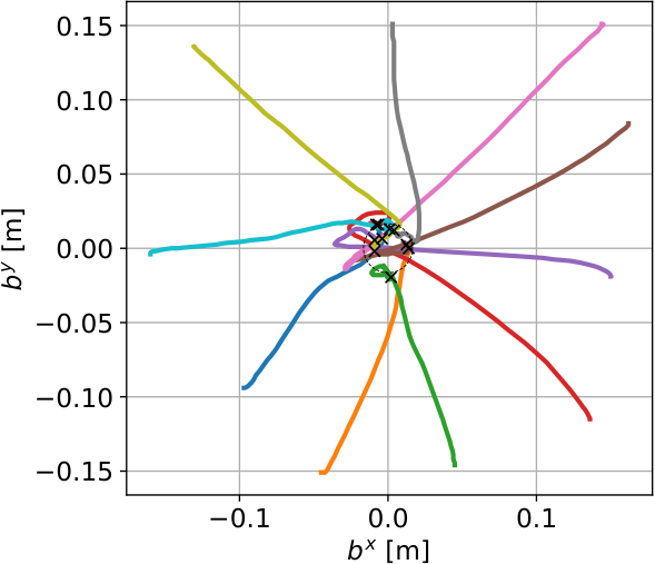
We tested the policy starting from ten different points in order to compare the two policies obtained by VF-MC-PILCO (Fig. 11) and MC-PILCO4PMS. The mean steady-state error, i.e. the average distance of the last ball position from the center observed in the ten tests, was 0.0134 [m], while MC-PILCO4PMS final policy obtained a slightly better result, with a mean error of 0.0099 [m]. This might be due to the difference between the two policy inputs: MC-PILCO4PM relies on a Kalman filter, while VF-MC-PILCO works directly with raw measurements (in presence of significant noise). Nevertheless, this performance difference is quite negligible, given the dimension of the ball whose radius is 0.016 [m].

References

- [1] Athanasios S Polydoros and Lazaros Nalpantidis. Survey of model-based reinforcement learning: Applications on robotics. Journal of Intelligent & Robotic Systems, 86(2):153–173, 2017.
- [2] Richard S Sutton and Andrew G Barto. Reinforcement learning: An introduction. MIT press, 2018.
- [3] Christopher G Atkeson and Juan Carlos Santamaria. A comparison of direct and model-based reinforcement learning. In Proceedings of international conference on robotics and automation, volume 4, pages 3557–3564. IEEE, 1997.
- [4] Christopher KI Williams and Carl Edward Rasmussen. Gaussian processes for machine learning. MIT press Cambridge, MA, 2006.
- [5] Marc Deisenroth and Carl E Rasmussen. Pilco: A model-based and data-efficient approach to policy search. In Proceedings of the 28th International Conference on machine learning (ICML-11), pages 465–472, 2011.
- [6] Marc Peter Deisenroth, Carl Edward Rasmussen, and Dieter Fox. Learning to control a low-cost manipulator using data-efficient reinforcement learning. Robotics: Science and Systems VII, pages 57–64, 2011.
- [7] Felix Berkenkamp, Matteo Turchetta, Angela Schoellig, and Andreas Krause. Safe model-based reinforcement learning with stability guarantees. In Advances in neural information processing systems, pages 908–918, 2017.
- [8] Konstantinos Chatzilygeroudis, Roberto Rama, Rituraj Kaushik, Dorian Goepp, Vassilis Vassiliades, and Jean-Baptiste Mouret. Black-box data-efficient policy search for robotics. In 2017 IEEE/RSJ International Conference on Intelligent Robots and Systems (IROS), pages 51–58. IEEE, 2017.
- [9] Kurtland Chua, Roberto Calandra, Rowan McAllister, and Sergey Levine. Deep reinforcement learning in a handful of trials using probabilistic dynamics models. In Advances in Neural Information Processing Systems, pages 4754–4765, 2018.
- [10] Thanard Kurutach, Ignasi Clavera, Yan Duan, Aviv Tamar, and Pieter Abbeel. Model-ensemble trust-region policy optimization. arXiv preprint arXiv:1802.10592, 2018.
- [11] Fabio Amadio, Alberto Dalla Libera, Riccardo Antonello, Daniel Nikovski, Ruggero Carli, and Diego Romeres. Model-based policy search using monte carlo gradient estimation with real systems application. IEEE Transactions on Robotics, 38(6):3879–3898, 2022.
- [12] D. Romeres, M. Zorzi, R. Camoriano, S. Traversaro, and A. Chiuso. Derivative-free online learning of inverse dynamics models. IEEE Transactions on Control Systems Technology, 28(3):816–830, 2020.
- [13] A. Dalla Libera, D. Romeres, D. K. Jha, B. Yerazunis, and D. Nikovski. Model-based reinforcement learning for physical systems without velocity and acceleration measurements. IEEE Robotics and Automation Letters, 5(2):3548–3555, 2020.
- [14] Marc Peter Deisenroth, Dieter Fox, and Carl Edward Rasmussen. Gaussian processes for data-efficient learning in robotics and control. IEEE transactions on pattern analysis and machine intelligence, 37(2):408–423, 2013.
- [15] Diego Romeres, Devesh K Jha, Alberto DallaLibera, Bill Yerazunis, and Daniel Nikovski. Semiparametrical gaussian processes learning of forward dynamical models for navigating in a circular maze. In 2019 International Conference on Robotics and Automation (ICRA), pages 3195–3202. IEEE, 2019.
- [16] Diederik P Kingma and Max Welling. Auto-encoding variational bayes. arXiv preprint arXiv:1312.6114, 2013.
- [17] Danilo Jimenez Rezende, Shakir Mohamed, and Daan Wierstra. Stochastic backpropagation and approximate inference in deep generative models. In International conference on machine learning, pages 1278–1286. PMLR, 2014.
- [18] Diederik P Kingma and Jimmy Ba. Adam: A method for stochastic optimization. arXiv preprint arXiv:1412.6980, 2014.
- [19] Adam Paszke, Sam Gross, Francisco Massa, Adam Lerer, James Bradbury, Gregory Chanan, Trevor Killeen, Zeming Lin, Natalia Gimelshein, Luca Antiga, Alban Desmaison, Andreas Kopf, Edward Yang, Zachary DeVito, Martin Raison, Alykhan Tejani, Sasank Chilamkurthy, Benoit Steiner, Lu Fang, Junjie Bai, and Soumith Chintala. Pytorch: An imperative style, high-performance deep learning library. Advances in Neural Information Processing Systems 32, pages 8024–8035, 2019.
- [20] Emanuel Todorov, Tom Erez, and Yuval Tassa. Mujoco: A physics engine for model-based control. In 2012 IEEE/RSJ International Conference on Intelligent Robots and Systems, pages 5026–5033. IEEE, 2012.
- [21] Benjamin Seth Cazzolato and Zebb Prime. On the dynamics of the furuta pendulum. Journal of Control Science and Engineering, 2011, 2011.