Are Random Decompositions all we need in High Dimensional Bayesian Optimisation?
Abstract
Learning decompositions of expensive-to-evaluate black-box functions promises to scale Bayesian optimisation (BO) to high-dimensional problems. However, the success of these techniques depends on finding proper decompositions that accurately represent the black-box. While previous works learn those decompositions based on data, we investigate data-independent decomposition sampling rules in this paper. We find that data-driven learners of decompositions can be easily misled towards local decompositions that do not hold globally across the search space. Then, we formally show that a random tree-based decomposition sampler exhibits favourable theoretical guarantees that effectively trade off maximal information gain and functional mismatch between the actual black-box and its surrogate as provided by the decomposition. Those results motivate the development of the random decomposition upper-confidence bound algorithm (RDUCB) that is straightforward to implement - (almost) plug-and-play - and, surprisingly, yields significant empirical gains compared to the previous state-of-the-art on a comprehensive set of benchmarks. We also confirm the plug-and-play nature of our modelling component by integrating our method with HEBO (Cowen-Rivers et al. 2022), showing improved practical gains in the highest dimensional tasks from the Bayesmark problem suite.
Keywords:
Machine Learning, ICML1 Introduction
Although Bayesian optimisation (BO) demonstrated impressive successes in low-dimensional domains (Marchant & Ramos 2012; Shahriari et al. 2015; Kandasamy et al. 2017; Kandasamy et al. 2018; Grosnit et al. 2022), scaling BO to high-dimensional and expensive to evaluate black-box functions has proved challenging. Among the many proposed approaches ranging from linear to non-linear projections (Wang et al. 2016; Rana et al. 2017; Li et al. 2018; Tripp et al. 2020; Moriconi et al. 2020; Eriksson & Jankowiak 2021; Grosnit et al. 2021b; Wan et al. 2021), decomposition methods that assume additively structured black-boxes emerged as a promising direction for high-dimensional BO (Kandasamy et al. 2015; Rolland et al. 2018; Han et al. 2021).
Given a decomposition in the dimensions of the problem, those techniques utilise additive kernel Gaussian processes (GPs) as surrogate models to trade off exploration and exploitation when suggesting novel queries to evaluate. Additive techniques uncover new inputs by maximising an acquisition function that is additive under the provided decomposition. Although first and second-order methods (Wilson et al. 2017) can be used to maximise acquisition functions, we adopt message-passing optimisers that can better exploit additive acquisition structures (Rolland et al. 2018).
The success of additive methods in high-dimensional BO depends on the correct choice of decompositions that must accurately mimic the inter-dimensional dependencies of the actual black-box function. Prior art empirically demonstrated that tree-structured decompositions (i.e., cycle-free pair-wise dimensional interactions) could effectively represent many black-box functions. The Tree algorithm (Han et al. 2021) discovers the best tree decomposition for the black-box based on the data collected during BO, by maximising a new GP marginal that includes decomposition parameters (encoding sparsity) and length scales.
At first glance, learning decompositions based on data and marginal likelihood is plausible and can yield promising optimisation results. While this is true when given a fixed dataset, dynamically acquired data during BO provides, at best, local (within the probed regions) function information, making it challenging to extrapolate dimensional interdependencies across the search space. In other words, such agents are easily misled by modifying the black-box function’s factorisation based on regions of the search space (for example see Section 3).
Contributions: Of course, one can think of many directions to resolve this issue, like analysing distribution shifts (Kirschner et al. 2020), maximising estimators beyond marginals (Ziegel 2003), or even designing novel Gaussian process kernels. In our work, however, we prefer to develop a simple (almost) plug-and-play approach that leads to empirical gains while adhering to rigorous theoretical guarantees. Therefore, rather than relying on data-driven learning, we investigate adopting data-independent decomposition rules. Our theoretical results indicate that random decomposition sampling strategies achieve the lowest expected mismatch to the black-box function when we fix the class of decompositions to trees, which allows us to favourably bound maximal information gain. Equipped with these results, we then propose the random decomposition upper-confidence bound (RDUCB) algorithm. RDUCB utilises a random tree sampler and an additive acquisition function to achieve superior empirical performance on a broad set of benchmarks compared to the prior state-of-the-art. The modelling component of RDUCB is simple to implement and thus easy to integrate on top of many existing BO frameworks. We support this claim by augmenting HEBO (Cowen-Rivers et al. 2022) - the winning submission of the NeurIPS 2020 black-box optimisation challenge (Turner et al. 2021) - with our random decomposition sampling strategy. We demonstrate that this adaptation, which we title RDHEBO, delivers improved performance on the set of highest dimensional Bayesmark (Asuncion & Newman 2007; Turner et al. 2021) tasks.
2 Background
2.1 Bayesian Optimisation (BO)
We employ a sequential decision-making approach to the maximisation of expensive-to-evaluate black-box functions over an input domain . At each round , we determine an input and observe its black-box function value . We allow noise-corrupted observations such that . Our goal is to approach the optimum, , rapidly as a function of black-box queries. Given that both the black-box function and optima are unknown, BO solvers trade-off exploration and exploitation via a two-step procedure involving fitting a surrogate model and maximising an acquisition function. We detail each of those steps below.
Gaussian Process Surrogates (GPs): GPs allow us to place priors directly in the function space by specifying a mean function and a covariance kernel that encode our assumptions about the black-box. Following (Williams & Rasmussen 2006), we assume a zero-mean and adopt a squared exponential covariance kernel:
where is a set of hyper-parameters tuned by maximising the data marginal11 1 In our equation, we execute element-wise..
Given the data collected so-far during BO rounds, we write the posterior at a point as with:
where concatenates all observations in one vector and represents an identity matrix. The matrix evaluates the covariance kernel on all input pairs in . Finally, the vector contains the kernel evaluation between and all input data points from .
Acquisition Function Maximisation: Given the posterior predictive distribution above, we now discuss how to suggest novel query points that improve the guess of the optima. In BO, this process involves maximising an acquisition function that utilises the probabilistic model such that . While there exist many acquisitions ranging from myopic to non-myopic forms (Frazier et al. 2008; Grosnit et al. 2021a; Cowen-Rivers et al. 2022; Shahriari et al. 2015; Zhang et al. 2021), in this paper, we follow (Srinivas et al. 2009; Srinivas et al. 2012) and adapt the upper-confidence bound as the function of choice:
where is a tuneable hyperparameter.
2.2 High-Dimensional BO with Decompositions
BO in high-dimensional spaces is an active area of research. In Section 6, we survey related methods to our work. In this section, we focus on decomposition-based strategies that promise to scale BO while accelerating acquisition optimisation. Before diving into the details of decomposition-based techniques, we now introduce the notion of decompositions of -dimensional spaces as follows:
Definition 2.1.
A decomposition of -dimensions is a collection of sets , called components, consisting of dimensions , i.e. .
Decomposition-based BO assumes that the black-box function decomposes according to : , where selects those dimensions of that appear in .
Additive GP Kernels: Compared to standard BO from Section 2.1, the first change decomposition methods employ is the usage of additive kernels (Duvenaud et al. 2011; Durrande et al. 2012; Qamar & Tokdar 2014; Lu et al. 2022) that better suit a decomposable black-box function: . Significantly, if two dimensions and do not appear together in any of the sets , the kernel will not model interactions between them. Rolland et al. 2018 showed that the posterior of each component subfunction can be expressed as , where:
where is a vector of kernel evaluations between and all inputs in while only considering those dimensions that appear in .
If the size of each set is much smaller than the total dimensionality , such an approach will enjoy many benefits. First, we escape the curse of dimensionality, as we only need to consider interactions between a small number of dimensions. Second, if we utilise an acquisition function with an additive structure, such as the additive UCB: we can determine novel query points to evaluate very efficiently using message passing (Rolland et al. 2018).
However, this is only possible if we know the decomposition of the black box. Existing methods attempt to learn it from data using maximum likelihood (Kandasamy et al. 2015; Rolland et al. 2018; Han et al. 2021), but there are no guarantees regarding the correctness of such a learning procedure. We expand on the problems associated with this approach in the next section.
3 Misleading Decomposition Learners
As noted in the previous section, decomposition methods learn the optimal additive kernel structure by selecting the one which produces a model with the highest marginal likelihood. While plausible and generally adopted, we now point out some problems associated with likelihood maximisation when learning decompositions in BO. Before we underpin this issue from a theoretical perspective, we first provide an empirical example that demonstrates those challenges next.
3.1 Challenges to Decompositions Learners
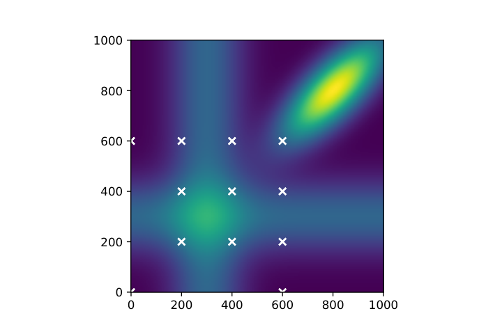
Consider the maximisation of the function demonstrated by the heat plot shown in Figure 1. It is easy to see that while this function is not fully separable due to the correlated mode in the top-right corner, it can locally appear as if it was entirely separable.
Imagine that we collected several initial points from the region and . Methods that rely entirely on data when learning the kernel structure (e.g., by maximising marginals) would exploit the local view of the function and falsely believe a complete separation in dimensions. We support this realisation in Figure 1 by running the state-of-the-art Tree algorithm from (Han et al. 2021) that learns decompositions via maximum likelihood.
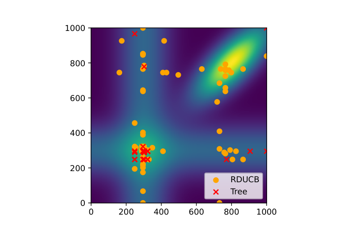
We see that the Tree algorithm gets stuck in the local mode because of erroneously learning that the function is fully decomposable. In contrast, our algorithm RDUCB, which we propose throughout the paper, circumvents this problem, whereby given the same initial design and settings of Tree, it can still find the optimal mode.
3.2 What Causes the Failure?
To better understand the above failure mode, we notice that approaches learning decompositions from data (e.g., Tree (Han et al. 2021)) assume that the function abides by one decomposition that does not vary across the search space, which is not the case in Figure 1.
To improve decomposition methods in high-dimensional BO, we wish to develop algorithms that enable varying decompositions across the search space. We could formalise this problem by imagining an adversary choosing a decomposition, , and a corresponding black-box function, , to optimise. This function must be a member of the reproducing kernel Hilbert space defined by some kernel , following the selected decomposition , unknown to the algorithm. It is important to note that such an adversary can select a black-box function that globally follows a decomposition but locally appears to have fewer interaction components than . As we cannot rely on locally collected data, we wish to investigate data-independent rules while ensuring a rigorous theoretical understanding.
On Data Independent Kernel Updates: Although we are the first to propose data-independent updates to select decompositions in BO, it is worth noting that the work in (Berkenkamp et al. 2019) already considered data-independent rules but when tuning kernel hyper-parameters with no focus on decompositions. The authors demonstrated no-regret bounds for an algorithm that alters the GP kernel’s hyperparameters according to a predefined scheme that does not rely on data gathered during BO.
However, the direct application of the work in (Berkenkamp et al. 2019) to learning decompositions is challenging for several reasons. First, our problem setting varies in that the authors in (Berkenkamp et al. 2019) consider low-dimensional BO that does not require learning kernel decompositions. Second and more importantly, the update rule in (Berkenkamp et al. 2019) keeps decreasing the length scales, expanding the kernel’s complexity as measured by maximum information gain (Srinivas et al. 2009), which will play a critical role in trading-off complexity versus mismatch as we note in Section 4.1.
Next, we expand on how to design such data-independent decomposition schemes and note that sparse random trees serve as a simple, effective, and scalable strategy.
4 Decompositions Without Learning
To better understand what properties constitute good predefined decomposition rules, we begin with a theoretical study that hints at the necessary trade-offs our strategy needs to optimise. Let us introduce to be a predefined (data-independent) scheme that selects a decomposition from some class of decompositions at each round . Consequently, defines the kernel that we use during that round .
We wish to derive a high-probability regret bound in terms of 1) a quantity roughly measuring the kernel’s complexity and 2) a notion of function mismatch between the true black-box and those functions spanned by our kernel . For kernel complexity, we follow (Srinivas et al. 2009) and use the maximum information gain of kernels defined by the decompositions proposed by our scheme22 2 Of course in (Srinivas et al. 2009) decompositions are not considered. Here, we define a slight generalisation of maximal information gain to handle the case of a changing kernel.. Here, denotes the maximum information gain after steps, where is a set of selected points and , where and . Concerning function mismatch, we define such that is the function from the reproducing kernel Hilbert space (RKHS) of kernel that is closest to the black-box in terms of infinity norm. This way provides a notion of mismatch between the actual black-box and the closest function from the RKHS of . Now, if we run a UCB-style BO algorithm for rounds, we obtain the following result.
Theorem 4.1.
Let the black-box function be selected by an adversary from an RKHS of kernel , defined over some decomposition that is also selected by an adversary. After rounds, a UCB-style BO algorithm with an decomposition rule, incurs with a probability of at least the following total cumulative regret :
where and denotes the norm in .
Proof.
(Sketch) We defer complete proof to Appendix A.1. Here, we provide a sketch of the main steps. BO under misspecification has been studied by (Bogunovic & Krause 2021). In their setting, the authors assume fixed kernels in-between iterations. Hence, we need to adapt the proof from (Bogunovic & Krause 2021) to our setting where the kernel and the mismatch vary. To do so, we observe that at any given time, the difference between and can be at most . Consequently, the difference between and becomes the new term that we bound. Here, we adapt a high probability bound to the case of a changing kernel. The final step of the proof is to express the bound in terms of maximum information gain , which easily follows from preceding BO literature (Srinivas et al. 2009). ∎
Note that is a random quantity. Thus to make this bound easier to analyse, we derive the following Corollary. We provide its proof in Appendix A.2.
Corollary 4.2.
Under the assumptions of Theorem 4.1, we have with probability at least , the cumulative regret of a UCB-style BO algorithm utilising the decomposition suggesting scheme , incurs the following cumulative regret:
4.1 Analysing Decomposition Rules
From Corollary 4.2, we notice that we need a decomposition rule such that both and are “small”. To bound , we require a restriction on the class of decompositions our scheme can propose. If we choose this class to consist only of decompositions with pairwise components, we get the following result on , proven in Appendix A.3.
Proposition 4.3.
The maximum information gain for a squared exponential kernel following a decomposition only with pair-wise components in dimensions is upper-bounded by .
In light of the result above, it might be tempting to try a decomposition with all possible pairwise components. However, given the empirical success of the Tree algorithm (Han et al. 2021), it appears that for many problems, it is sufficient to consider tree-structured decompositions, which we now proceed to define.
Definition 4.4.
A decomposition is tree-based with edges if it has pair-wise components and the remaining components contain one dimension. Additionally, an undirected graph formed by edges corresponding to pair-wise interactions does not contain a cycle.
If we restrict ourselves to the class of trees, we additionally reduce the maximum information gain, as stated by the next result, proven in Appendix A.4.
Proposition 4.5.
When , the maximum information gain for a kernel following a tree decomposition (possibly changing between timesteps) is always smaller than for a kernel containing all pairwise interactions.
Bounding Expected Mismatches : Bounding is far more challenging. To understand this difficulty, let us consider two extremes when suggesting decompositions: constant and adaptive decomposition selection rules . If constantly suggests the same decomposition, the adversary efficiently exploits this strategy resulting in a constant high mismatch. While if we adaptively increase the kernel’s complexity using procedures like those in (Berkenkamp et al. 2019), our method will indeed reduce mismatch regardless of the adversary’s choices. However, as we introduce more interactions between dimensions, our decompositions eventually stop being trees and thus lead to increases in information gain .
Analysing the bound above, we observe a trade-off between maximal information gain and the risk of being exploited by an adversary. To resolve this problem, we propose to use a randomised tree sampling strategy that keeps the information gain small while circumventing adversaries. Importantly, we show that such an exhibits the lowest expected mismatch within a class of tree-structured decompositions. We now state the formal result.
Theorem 4.6.
Let be a class of -dimensional tree-based decompositions with edges. Let the adversary choose any function from RKHS defined by kernel on a decomposition also chosen by the adversary, such that the infinity norm of each component function is bounded and . We then have that for any data-independent scheme , the expected sum of mismatches is at least as large as for the scheme that selects a decomposition from uniformly at random, i.e.,
Proof.
(Sketch) We defer complete proof to Appendix A.5. Observe that the optimal strategy for an adversary is to put all the mismatch on the pair-wise component least selected by the scheme . Since we will suffer a mismatch of every time we do not select this component, the optimal scheme needs to maximise the expected number of times the least selected component is chosen. This happens when all pair-wise components have the same probability of being selected, proving the optimality of . ∎
4.2 Practical Algorithm: Random Decompositions UCB
Equipped with the above results, this section presents a practical and effective algorithm for high-dimensional BO. Our algorithm, titled random decomposition upper confidence bound (RDUCB), adheres to the theoretical results from the previous section and allows a scalable implementation.
Algorithm 1 is a pseudo code of RDUCB. At a high-level, our method follows any generic BO solver in that it first fits a probabilistic model (line 5) and then maximises an acquisition, as shown in line 6. Of course, we maximise additive UCB acquisitions as dictated by the sampled decomposition . As noted earlier, decompositions correspond to trees that we sample so that each edge has an equal probability of being selected. We present this sampler (referred to in line 4 of Algorithm 1) in Algorithm 2 in Appendix B.
5 Empirical Evaluation
This section presents experimental results on multiple benchmarks. We compare RDUCB against well-established techniques, including tree-based learners (Han et al. 2021), random embedding BO (Wang et al. 2013), Hashing-enhanced Subspace Bayesian Optimization (HeSBO) (Nayebi et al. 2019), Coordinate Line BO (Kirschner et al. 2019) and random search33 3 It is worth noting that REMBO, HeSBO and CoordinateLineBO are presented in all experiments except those involving neural architecture search (NAS). The reason is that NAS baselines operate in discrete search spaces for which these algorithms are not well-suited.. The comparison against tree-learning-based BO allows us to gauge improvements compared to the prior state-of-the-art. In contrast, the comparison to REMBO, HeSBO and LineBO sheds light on the advantages we gain when operating in the original high-dimensional space.
In Appendix C, we provide all algorithm settings used in our experiments. We have open-sourced our code44 4 https://github.com/huawei-noah/HEBO/tree/master/RDUCB to ease the reproducibility of our results.
5.1 Benchmark Datasets
Synthethic Functions: We test our method on 20-dimensional Rosebrock, 20-dimensional Hartmann, and 250-dimensional Styblinski-Tang (Stybtang) functions. We calculate the regret as the difference between queried function value and the theoretical minimum.
Neural Network Hyperparameter Tuning: In the second set of experiments, we consider the neural architecture search (NAS) hyperparameter tuning benchmark (Zela et al. 2020). This benchmark consists of precomputed validation mean-squared errors for different combinations of hyperparameters in a two-layer feed-forward neural network trained on four different datasets. This experiment considers mixed search spaces, e.g., learning and drop-out rates (continuous), the sizes of hidden layers and activation types (discrete).
Mixed Integer Programming: We consider the problem of tuning heuristic hyperparameters for the mixed integer programming (MIP) solver LPSolve (Berkelaar et al. 2015). This domain is high-dimensional with a 74-dimensional search space. We consider three MIP problems varying in difficulty with the misc05inf instance being the hardest. For each problem, the regret value is the duality gap of the best solution found after 5 seconds with given hyperparameters. We cap the maximum instantaneous regret at 500, and running the solver once is considered as one query.
Weighted Lasso Tuning: The last problem we consider is tuning the LassoBench (Šehić et al. 2022). LassoBench is a set of benchmark problems where BO tunes the weights for a weighted Lasso model. Hence, the number of dimensions of the search space scales with the number of features in the dataset. The highest dimension we study in this experiment is the 180 DNA data.
5.2 Regret Results
We run all algorithms varying the number of seeds per-each benchmark to allow for statistically significant results on the tasks introduced above. We report some of these results in this section (Figures 3 and 3) and defer others to Appendix E due to space constraints. Every algorithm started with 10 initial randomly sampled points. Note that for HeSBO, the initial points were sampled in the algorithm’s lower-dimensional space (hence the initial regret is sometimes different from other algorithms).
In general, we notice that RDUCB outperforms other baselines. We see that our improvements are amplified in high dimensional settings, as reported in Figures 3(a) and Figures 3(a), 3(b) and 3(c). In three experiments, RDUCB draws in terms of final regret with Tree, and in two benchmarks RDUCB (minorly) underperforms compared to Tree (see Appendix E). We note that the cases when RDUCB draws or underperforms mostly correspond to low-dimensional settings. We expand on this in the next section.
5.3 Scalability as Dimensionalities Increase
We conduct an ablation study to test how our method scales with the number of dimensions and to understand its potential limitations. We choose one synthetic function and one real-world problem. For the synthetic function, we vary the dimensionality of the Stybtang function, while in the real-world case, we tackle the LassoBench DNA problem. For the latter, we produce different versions of this problem with varying dimensionalities. To achieve this, we turn some dimensions off by permanently setting them to zero and allowing the algorithm to vary only the remaining ones.
We compare the best regret achieved by the algorithm in (Han et al. 2021) (titled Tree in the figure) and RDUCB after 500 iterations for Stybtang and 700 iterations for LassoBench DNA, respectively. We show the results of ablation in Figure 4. Although for a small number of dimensions, Tree can slightly outperform RDUCB, we see that as the number of dimensions increases, RDUCB starts to outperform, and the gap widens for higher-dimensional problems.
5.4 Plug-and-Play for RDHEBO
RDUCB presents a simple modification strategy to modelling using GPs, allowing it to plug on top of existing BO algorithms. This section supports our claim by introducing RDHEBO, an adaptation of HEBO (Cowen-Rivers et al. 2022) that uses our random decomposition scheme. We keep all the other components (warping functions and multi-objective acquisitions) of HEBO unchanged and present a comparison conducted on the highest dimensional Bayesmark tasks in Table 1. We can see that our modification has improved the performance of HEBO across those tasks, rising from a score of 92.68 to 93.67 in the MLP-Adam task, for instance.
| Problem | HEBO | RDHEBO |
|---|---|---|
| MLP-Adam | ||
| MLP-SGD | ||
| DT | ||
| RF | ||
| Average |
6 Related Work
Random projection methods project the inputs from a high dimensional space to a space of lower dimensionality by randomised mappings. To do so, REMBO (Wang et al. 2013) uses a matrix with entries sampled from a normal distribution. Though successful, REMBO tends to over-explore regions that are on the boundary of the domain of the black-box function. The authors in (Letham et al. 2020) proposed ALEBO, an algorithm that addresses some of REMBO’s problems, while Nayebi et al. 2019 use different projection types altogether. The algorithm they propose - HeSBO, initialises a randomised hashing function that maps back to the original space, leading to improved results. As opposed to all those techniques, RDUCB takes a different direction of decomposing the original space rather than projecting to lower dimensional manifolds.
LineBO methods (Kirschner et al. 2019) conduct optimisation over an affine, one-dimensional subspace. This subspace is chosen so that the best point found so far belongs to it. There are different variants of LineBO, where the direction of this one-dimensional space is chosen randomly (Random LineBO), aligned with a randomly chosen dimension (Coordinate LineBO) or along a gradient estimate (Descent LineBO). We chose to compare RDUCB with Coordinate LineBO, as in most cases it outperforms other LineBO variants.
Latent space methods perform the optimisation in some latent space and then utilise a generative model as a projection to original space. A commonly taken approach is to utilise the latent space of a Variational AutoEncoder (Kingma & Welling 2013), pretrained on some larger batch of existing data. However, over the course of this pretraining, we need to ensure that the obtained latent space is well-suited for BO. There have been numerous VAE-based algorithms proposed (Eissman et al. 2018; Gómez-Bombarelli et al. 2018; Zhang et al. 2019; Tripp et al. 2020; Griffiths & Hernández-Lobato 2020; Siivola et al. 2021; Grosnit et al. 2021b), employing various mechanisms to achieve this goal.
While using deep networks to scale BO is prominent and essential, RDUCB constitutes an orthogonal research direction where our discoveries, at least in the modelling component, can (easily) plug-and-play in latent spaces, e.g., when using deep kernel GPs (Wilson et al. 2016) in general. We instantiated one such plug-and-play use-case in this paper (see Section 5.4) and planned to further investigate such applications in the future.
Dropout methods (Li et al. 2017) randomly drop several dimensions and optimise only a subset at each step. When querying for new values of the black-box function, the value of dimensions that were not optimised at a given iteration are selected according to some filling strategy that can either copy the value of the best point so far or choose a random value. Though successful in isolated instances, dropout methods exhibit high-sample complexity.
SAASBO (Eriksson & Jankowiak 2021) adopts a hierarchical Bayesian model, putting a prior on the length scale with a high probability mass concentrated at zero. Hence, a dimension will be effectively removed from the model unless there is enough evidence that it dramatically impacts the black-box function value.
Trust region methods tackle high dimensional spaces by optimising locally within a chosen trust region. The TuRBO algorithm (Eriksson et al. 2019) maintains several trust regions and selects one at a given time using a multi-armed bandit strategy. CASMOPOLITAN (Wan et al. 2021) extends this idea to handle categorical and mixed input spaces.
Our research in this paper is orthogonal to SAASBO and trust region methods. In the future, we plan to integrate our modelling component with the works in (Eriksson et al. 2019) and (Eriksson & Jankowiak 2021).
7 Discussion & Future Work
This paper introduced random decompositions to scale BO to high-dimensional spaces. Our algorithm, RDUCB, is simple to implement, empirically effective and theoretically grounded. We compared our method against the prior decomposition state-of-the-art technique and showed improved best-regret results on a wide set of publicly available benchmarks. While this is the first step in understanding data-independent rules for high dimensional BO, there is a number of challenges that we now elaborate on.
Currently, RDUCB is not capable of handling non-numerical inputs (e.g., graphs or strings). This problem is not only tied to RDUCB but also challenges other decomposition-based techniques since we cannot easily define a notion of decomposition for such input types. We plan to investigate such decomposition rules in the future.
Apart from tackling technical challenges, in the future, we plan to scale RDUCB to thousands of dimensions. We hope to benefit from distributed and high-performance computing. Of course, this direction requires us to devise novel consensus-based acquisition optimisers, which have recently seen progress in non-convex settings (Zhang et al. 2022).
Although we applied the modelling component of RDUCB to HEBO, we believe many BO frameworks and algorithms can benefit from our decomposition scheme. Those include trust-region methods, latent space techniques, and combinatorial BO solvers. In the future, we will also investigate this direction in combination with scalability.
References
- Asuncion & Newman (2007) Asuncion, A. and Newman, D. Uci machine learning repository, 2007.
- Berkelaar et al. (2015) Berkelaar, M. et al. Package ‘lpsolve’, 2015.
- Berkenkamp et al. (2019) Berkenkamp, F., Schoellig, A. P., and Krause, A. No-regret bayesian optimization with unknown hyperparameters. arXiv preprint arXiv:1901.03357, 2019.
- Bogunovic & Krause (2021) Bogunovic, I. and Krause, A. Misspecified gaussian process bandit optimization. Advances in Neural Information Processing Systems 34, 2021.
- Chowdhury & Gopalan (2017) Chowdhury, S. R. and Gopalan, A. On kernelized multi-armed bandits. In International Conference on Machine Learning, pp. 844–853. PMLR, 2017.
- Cowen-Rivers et al. (2022) Cowen-Rivers, A. I., Lyu, W., Tutunov, R., Wang, Z., Grosnit, A., Griffiths, R. R., Maraval, A. M., Jianye, H., Wang, J., Peters, J., et al. Hebo: pushing the limits of sample-efficient hyper-parameter optimisation. Journal of Artificial Intelligence Research, 74:1269–1349, 2022.
- Durrande et al. (2012) Durrande, N., Ginsbourger, D., and Roustant, O. Additive covariance kernels for high-dimensional gaussian process modeling. In Annales de la Faculté des sciences de Toulouse: Mathématiques, volume 21, pp. 481–499, 2012.
- Duvenaud et al. (2011) Duvenaud, D. K., Nickisch, H., and Rasmussen, C. Additive gaussian processes. Advances in neural information processing systems, 24, 2011.
- Eissman et al. (2018) Eissman, S., Levy, D., Shu, R., Bartzsch, S., and Ermon, S. Bayesian optimization and attribute adjustment. In Proc. 34th Conference on Uncertainty in Artificial Intelligence, 2018.
- Eriksson & Jankowiak (2021) Eriksson, D. and Jankowiak, M. High-dimensional bayesian optimization with sparse axis-aligned subspaces. In Uncertainty in Artificial Intelligence, pp. 493–503. PMLR, 2021.
- Eriksson et al. (2019) Eriksson, D., Pearce, M., Gardner, J., Turner, R. D., and Poloczek, M. Scalable global optimization via local bayesian optimization. Advances in neural information processing systems, 32, 2019.
- Frazier et al. (2008) Frazier, P. I., Powell, W. B., and Dayanik, S. A knowledge-gradient policy for sequential information collection. SIAM Journal on Control and Optimization, 47(5):2410–2439, 2008.
- Gómez-Bombarelli et al. (2018) Gómez-Bombarelli, R., Wei, J. N., Duvenaud, D., Hernández-Lobato, J. M., Sánchez-Lengeling, B., Sheberla, D., Aguilera-Iparraguirre, J., Hirzel, T. D., Adams, R. P., and Aspuru-Guzik, A. Automatic chemical design using a data-driven continuous representation of molecules. ACS central science, 4(2):268–276, 2018.
- Griffiths & Hernández-Lobato (2020) Griffiths, R.-R. and Hernández-Lobato, J. M. Constrained bayesian optimization for automatic chemical design using variational autoencoders. Chemical science, 11(2):577–586, 2020.
- Grosnit et al. (2021a) Grosnit, A., Cowen-Rivers, A. I., Tutunov, R., Griffiths, R.-R., Wang, J., and Bou-Ammar, H. Are we forgetting about compositional optimisers in bayesian optimisation? The Journal of Machine Learning Research, 22(1):7183–7260, 2021a.
- Grosnit et al. (2021b) Grosnit, A., Tutunov, R., Maraval, A. M., Griffiths, R.-R., Cowen-Rivers, A. I., Yang, L., Zhu, L., Lyu, W., Chen, Z., Wang, J., et al. High-dimensional bayesian optimisation with variational autoencoders and deep metric learning. arXiv preprint arXiv:2106.03609, 2021b.
- Grosnit et al. (2022) Grosnit, A., Malherbe, C., Tutunov, R., Wan, X., Wang, J., and Ammar, H. B. Boils: bayesian optimisation for logic synthesis. In 2022 Design, Automation & Test in Europe Conference & Exhibition (DATE), pp. 1193–1196. IEEE, 2022.
- Han et al. (2021) Han, E., Arora, I., and Scarlett, J. High-dimensional bayesian optimization via tree-structured additive models. In Proceedings of the AAAI Conference on Artificial Intelligence, volume 35, pp. 7630–7638, 2021.
- Kandasamy et al. (2015) Kandasamy, K., Schneider, J., and Póczos, B. High dimensional bayesian optimisation and bandits via additive models. In International conference on machine learning, pp. 295–304. PMLR, 2015.
- Kandasamy et al. (2017) Kandasamy, K., Dasarathy, G., Schneider, J., and Póczos, B. Multi-fidelity bayesian optimisation with continuous approximations. In International Conference on Machine Learning, pp. 1799–1808. PMLR, 2017.
- Kandasamy et al. (2018) Kandasamy, K., Krishnamurthy, A., Schneider, J., and Póczos, B. Parallelised bayesian optimisation via thompson sampling. In International Conference on Artificial Intelligence and Statistics, pp. 133–142. PMLR, 2018.
- Kingma & Welling (2013) Kingma, D. P. and Welling, M. Auto-encoding variational bayes. arXiv preprint arXiv:1312.6114, 2013.
- Kirschner et al. (2019) Kirschner, J., Mutny, M., Hiller, N., Ischebeck, R., and Krause, A. Adaptive and safe bayesian optimization in high dimensions via one-dimensional subspaces. In International Conference on Machine Learning, pp. 3429–3438. PMLR, 2019.
- Kirschner et al. (2020) Kirschner, J., Bogunovic, I., Jegelka, S., and Krause, A. Distributionally robust bayesian optimization. In International Conference on Artificial Intelligence and Statistics, pp. 2174–2184. PMLR, 2020.
- Letham et al. (2020) Letham, B., Calandra, R., Rai, A., and Bakshy, E. Re-examining linear embeddings for high-dimensional bayesian optimization. Advances in neural information processing systems, 33:1546–1558, 2020.
- Li et al. (2017) Li, C., Gupta, S., Rana, S., Nguyen, V., Venkatesh, S., and Shilton, A. High dimensional bayesian optimization using dropout. In Proceedings of the 26th International Joint Conference on Artificial Intelligence, pp. 2096–2102, 2017.
- Li et al. (2018) Li, C., Gupta, S., Rana, S., Nguyen, V., Venkatesh, S., and Shilton, A. High dimensional bayesian optimization using dropout. arXiv preprint arXiv:1802.05400, 2018.
- Lu et al. (2022) Lu, X., Boukouvalas, A., and Hensman, J. Additive gaussian processes revisited. In International Conference on Machine Learning, pp. 14358–14383. PMLR, 2022.
- Marchant & Ramos (2012) Marchant, R. and Ramos, F. Bayesian optimisation for intelligent environmental monitoring. In 2012 IEEE/RSJ international conference on intelligent robots and systems, pp. 2242–2249. IEEE, 2012.
- Moriconi et al. (2020) Moriconi, R., Deisenroth, M. P., and Sesh Kumar, K. High-dimensional bayesian optimization using low-dimensional feature spaces. Machine Learning, 109(9):1925–1943, 2020.
- Nayebi et al. (2019) Nayebi, A., Munteanu, A., and Poloczek, M. A framework for bayesian optimization in embedded subspaces. In International Conference on Machine Learning, pp. 4752–4761. PMLR, 2019.
- Nguyen et al. (2017) Nguyen, V., Gupta, S., Rana, S., Li, C., and Venkatesh, S. Regret for expected improvement over the best-observed value and stopping condition. In Asian conference on machine learning, pp. 279–294. PMLR, 2017.
- Qamar & Tokdar (2014) Qamar, S. and Tokdar, S. T. Additive gaussian process regression. arXiv preprint arXiv:1411.7009, 2014.
- Rana et al. (2017) Rana, S., Li, C., Gupta, S., Nguyen, V., and Venkatesh, S. High dimensional bayesian optimization with elastic gaussian process. In International conference on machine learning, pp. 2883–2891. PMLR, 2017.
- Rolland et al. (2018) Rolland, P., Scarlett, J., Bogunovic, I., and Cevher, V. High-dimensional bayesian optimization via additive models with overlapping groups. In International conference on artificial intelligence and statistics, pp. 298–307. PMLR, 2018.
- Šehić et al. (2022) Šehić, K., Gramfort, A., Salmon, J., and Nardi, L. Lassobench: A high-dimensional hyperparameter optimization benchmark suite for lasso. In International Conference on Automated Machine Learning, pp. 2–1. PMLR, 2022.
- Shahriari et al. (2015) Shahriari, B., Swersky, K., Wang, Z., Adams, R. P., and De Freitas, N. Taking the human out of the loop: A review of bayesian optimization. Proceedings of the IEEE, 104(1):148–175, 2015.
- Siivola et al. (2021) Siivola, E., Paleyes, A., González, J., and Vehtari, A. Good practices for bayesian optimization of high dimensional structured spaces. Applied AI Letters, 2(2):e24, 2021.
- Srinivas et al. (2009) Srinivas, N., Krause, A., Kakade, S. M., and Seeger, M. Gaussian process optimization in the bandit setting: No regret and experimental design. arXiv preprint arXiv:0912.3995, 2009.
- Srinivas et al. (2012) Srinivas, N., Krause, A., Kakade, S. M., and Seeger, M. W. Information-theoretic regret bounds for gaussian process optimization in the bandit setting. IEEE transactions on information theory, 58(5):3250–3265, 2012.
- Tripp et al. (2020) Tripp, A., Daxberger, E., and Hernández-Lobato, J. M. Sample-efficient optimization in the latent space of deep generative models via weighted retraining. Advances in Neural Information Processing Systems, 33:11259–11272, 2020.
- Turner et al. (2021) Turner, R., Eriksson, D., McCourt, M., Kiili, J., Laaksonen, E., Xu, Z., and Guyon, I. Bayesian optimization is superior to random search for machine learning hyperparameter tuning: Analysis of the black-box optimization challenge 2020. In NeurIPS 2020 Competition and Demonstration Track, pp. 3–26. PMLR, 2021.
- Wan et al. (2021) Wan, X., Nguyen, V., Ha, H., Ru, B., Lu, C., and Osborne, M. A. Think global and act local: Bayesian optimisation over high-dimensional categorical and mixed search spaces. arXiv preprint arXiv:2102.07188, 2021.
- Wang et al. (2013) Wang, Z., Zoghi, M., Hutter, F., Matheson, D., De Freitas, N., et al. Bayesian optimization in high dimensions via random embeddings. In IJCAI, volume 13, pp. 1778–1784, 2013.
- Wang et al. (2016) Wang, Z., Hutter, F., Zoghi, M., Matheson, D., and De Feitas, N. Bayesian optimization in a billion dimensions via random embeddings. Journal of Artificial Intelligence Research, 55:361–387, 2016.
- Williams & Rasmussen (2006) Williams, C. K. and Rasmussen, C. E. Gaussian processes for machine learning, volume 2. MIT press Cambridge, MA, 2006.
- Wilson et al. (2016) Wilson, A. G., Hu, Z., Salakhutdinov, R., and Xing, E. P. Deep kernel learning. In Artificial intelligence and statistics, pp. 370–378. PMLR, 2016.
- Wilson et al. (2017) Wilson, J. T., Moriconi, R., Hutter, F., and Deisenroth, M. P. The reparameterization trick for acquisition functions. arXiv preprint arXiv:1712.00424, 2017.
- Zela et al. (2020) Zela, A., Siems, J., and Hutter, F. Nas-bench-1shot1: Benchmarking and dissecting one-shot neural architecture search. arXiv preprint arXiv:2001.10422, 2020.
- Zhang et al. (2019) Zhang, M., Li, H., and Su, S. High dimensional bayesian optimization via supervised dimension reduction. arXiv preprint arXiv:1907.08953, 2019.
- Zhang et al. (2021) Zhang, Y., Zhang, X., and Frazier, P. Constrained two-step look-ahead bayesian optimization. Advances in Neural Information Processing Systems, 34:12563–12575, 2021.
- Zhang et al. (2022) Zhang, Y., Li, X., and Wang, L. Distributed h-infinity consensus of heterogeneous multi-agent systems with nonconvex constraints. ISA transactions, 131:160–166, 2022.
- Ziegel (2003) Ziegel, E. R. The elements of statistical learning, 2003.
Appendix A Proofs of Theoretical Results
A.1 Proof of Theorem 4.1
See 4.1
Proof.
Without the loss of generality, we assume kernel for every decomposition is normalised, i.e. and that our function observations are corrupted by some -subgaussian noise. Our proof follows the idea of the proof of Theorem 1 from (Bogunovic & Krause 2021), with some differences. Let be the kernel defined by decomposition selected at time . be a function living in RKHS of kernel that is closest to the true function measured by the infinity norm. To avoid clutter we will write and . Let be the vector of corrupted observations generated by , i.e. for some -subgaussian noise . Then let us define as the Gaussian Process posterior utilising kernel , which uses observations , i.e.:
In contrast, the mean computed by the algorithm uses the full observations from the true black-box function , without knowing which part came from . Let us assume, we run a UCB-style BO algorithm, with an acquisition function that we will define later. Let be the maximiser of black-box function. If we now look at the instantaneous regret, we get:
| (1) |
where the last inequality is due to the fact that and . Consequently, becomes the new term we need to bound. We now observe the following:
Hence, we would like to bound the differences and . To do so, we recall two lemmas from existing literature.
Lemma A.1 (Adapted Theorem 2 from (Chowdhury & Gopalan 2017)).
Let , and be a member of the RKHS of real-valued functions on with kernel defined by , where can be changed at each , with RKHS norm bounded by . Let the observations be corrupted by some -subgaussian noise. Then, with probability at least , the following holds for all :
Proof.
The proof is identical to the proof of Theorem 2 in (Chowdhury & Gopalan 2017), except that now the kernel depends on time.
∎
Lemma A.2 (Lemma 2 from (Bogunovic & Krause 2021)).
For any and , we have
where .
We adopt the notation . Following up on Inequality 1, by Lemmas A.1 and A.2 with probability at least , we get that the cumulative regret admits the following upper bound:
where we have introduced defined as:
| (2) |
Let us now define the acquisition rule of our BO algorithm as , where
By the acquisition rule, if point was selected, then and so:
Substituting the definition of (Eq. 2) we get:
We now observe that by Cauchy-Schwarz we have and
. We thus obtain the following bound:
Observe that , where and by Lemma 5.3 of (Srinivas et al. 2009), we have . We thus obtain:
since due to , we have .
∎
A.2 Proof of Corollary 4.2
See 4.2
Proof.
Using Markov’s inequality we have: . We now combine this fact with the bound developed in Theorem 4.1 and combine the probabilities using union bound to arrive at the corollary’s statement. ∎
A.3 Proof of Proposition 4.3
See 4.3
Proof.
As shown in (Rolland et al. 2018), for an additive squared exponential kernel in dimensional space, such that each subkernel operates on at most dimensions, we get that the maximum information gain is bounded as:
We observe that in our case and , which finishes the proof. ∎
A.4 Proof of Proposition 4.5
See 4.5
Proof.
We will denote by the class of all possible tree decompositions in dimensions. As such is the set of all pairwise components. Additionally, we will introduce the following notation:
where the quantities have the following distribution for all and all :
For some fixed sequence , we will write and and equivalently for and . By properties of mutual information, we have:
where the last inequality is true, as the conditional distributions are the same. Using the formula for the entropy of multivariate Gaussian we get:
where means the -th largest eigenvalue of and the covariance matrices are defined as and . We can thus write , where . One can easily see that must be PSD, as such we have , as adding a PSD matrix to another PSD matrix can never decrease its eigenvalues. This gives us:
with equality if and only if , which can happen only if all eigenvalues of are zero, meaning , i.e. all components are included at every step. This can only happen if there is only one decomposition in the class . As our class consist of trees, this is only possible when . ∎
A.5 Proof of Theorem 4.6
See 4.6
Proof.
We start by introducing the following lemma.
Lemma A.3.
Let be the true tree-based decomposition of and for some set of omitted pair-wise components . Then we have:
Proof.
where the first inequality is due to the triangle inequality and second due to the fact that and . ∎
Let us now define the probability of choosing a decomposition at time by our decomposition proposing scheme as . A deterministic scheme will just be a special case of the probabilistic scheme, where all probability is concentrated on one decomposition. Instead of thinking about the adversary as selecting a function , we can think about them as selecting the norm parameters for each pair-wise component , with the constraint that . Since the adversary knows the scheme, in the worst case they can select the decomposition and function so that the expected mismatch is maximal. This corresponds to:
where the last equality is due to Lemma A.3 and the fact that the adversary, in the worst case, will choose a function with the highest possible mismatch. We can now exchange the order of summation to obtain:
where is the expected number of time that a pair-wise component is not included in the proposed decomposition. Note that the expression above is maximised subject to the constraint that . Thus the maximum is achieved when the biggest mismatch is placed on the pair-wise component that is on average least selected. Formally, let , then the solution to the constrained maximization problem above is and can be any decomposition including . We thus obtain:
This is minimised, when for the selected scheme the expected number of times the least selected pair-wise component is not selected is minimal. This happens when the chance to include each of the pair-wise components is the same. Since all of the decompositions have the same number of pair-wise components, this corresponds to a uniform distribution over all trees. This proves the claim that a uniformly random scheme achieves the smallest expected mismatch. Under the uniformly random scheme, we select pair-wise components at each time out of all possible , so the probability of any one component being selected is and the inverse event has a probability of . Since the scheme is the same across all timesteps we get .
∎
Appendix B Procedure for Sampling random Trees
Appendix C Algorithm Settings
In Table 2, we detail settings used by each algorithm. Those values are used for all of the experiments.
| Algorithm | Setting | Value |
| Tree | Acquisition function | Additive UCB with |
| Decomposition learning interval | 15 | |
| Gibbs sampling iterations | 100 | |
| RDUCB | Acquisition function | Additive UCB with |
| Size of random tree | ||
| HeSBO | Acquisition function | EI (Nguyen et al. 2017) |
| Size of embedding | ||
| REMBO/ CoordinateLineBO | All | Default values from here |
C.1 Computing Resources
All experiments were run on machines with specifications described in Table 3.
| Component | Description |
|---|---|
| CPU | Intel Core i9-9900X CPU @ 3.50GHz |
| GPU | Nvidia RTX 2080 |
| Memory | 64 GB DDR4 |
Appendix D Toy problem details
In this section, we describe the details of the toy problem introduced in Section 3. For this experiment, we use algorithm setting as per Table 2. The function we use is three-dimensional, where the last dimension is redundant. Thus, in Figure 1 we only plot it as a function of two variables. We chose to add one redundant dimension as otherwise, RDUCB will always be sampling the same decomposition (size of random tree ). The formula for the function is given below:
where is a -dimensional Gaussian PDF defined on dimensions in with mean and covariance matrix . For the toy problem, we used the numerical values shown below.
Thus, there are two local optima for and , suboptimal at and global at . Variable can be set to any value, as it does not affect the function output. The initial points given to both Tree and RDUCB were exactly the same. We show them in Figure 5 below.