footnoteinfo]This research has been partially supported by the Progetto di Ateneo CPDA147754/14-New statistical learning approach for multi-agents adaptive estimation and coverage control, the project Deep probabilistic regression – new models and learning algorithms (contract number: 2021-04301), funded by the Swedish Research Council, the Wallenberg AI, Autonomous Systems and Software Program (WASP) funded by Knut and Alice Wallenberg Foundation and by Kjell och Märta Beijer Foundation. This paper was not presented at any IFAC meeting. Corresponding author Gianluigi Pillonetto Ph. +390498277607.
Deep networks for system identification: a survey
Abstract
Deep learning is a topic of considerable current interest. The availability of massive data collections and powerful software resources has led to an impressive amount of results in many application areas that reveal essential but hidden properties of the observations. System identification learns mathematical descriptions of dynamic systems from input-output data and can thus benefit from the advances of deep neural networks to enrich the possible range of models to choose from. For this reason, we provide a survey of deep learning from a system identification perspective. We cover a wide spectrum of topics to enable researchers to understand the methods, providing rigorous practical and theoretical insights into the benefits and challenges of using them. The main aim of the identified model is to predict new data from previous observations. This can be achieved with different deep learning based modelling techniques and we discuss architectures commonly adopted in the literature, like feedforward, convolutional, and recurrent networks. Their parameters have to be estimated from past data trying to optimize the prediction performance. For this purpose, we discuss a specific set of first-order optimization tools that is emerged as efficient. The survey then draws connections to the well-studied area of kernel-based methods. They control the data fit by regularization terms that penalize models not in line with prior assumptions. We illustrate how to cast them in deep architectures to obtain deep kernel-based methods. The success of deep learning also resulted in surprising empirical observations, like the counter-intuitive behaviour of models with many parameters. We discuss the role of overparameterized models, including their connection to kernels, as well as implicit regularization mechanisms which affect generalization, specifically the interesting phenomena of benign overfitting and double-descent. Finally, we highlight numerical, computational and software aspects in the area with the help of applied examples.
{daniel.gedon, antonio.horta.ribeiro, thomas.schon}@it.uu.se)††address: Department of Electrical Engineering, Linköping University, Linköping, Sweden (e-mail: lennart.ljung@liu.se)
1 Introduction
The term system identification was coined in the late 1950s by Zadeh in [352]. His seminal work set up a framework where mathematical laws governing dynamic systems are built starting from input-output measurements [268]. Since then, system identification has enjoyed many theoretical developments, becoming a key subfield of Automatic Control with several applications in science and engineering [190]. Despite its long history, research in data-based dynamical modeling is still extremely active. Many complex physical processes, arising e.g. in biology and industry, require an increasingly deep knowledge for improved prediction and control. This often requires handling high-dimensional data, posing new challenges. In addition, recently there has been a lot of interesting cross-fertilization between system identification and other areas, including machine learning and Bayesian statistics, with developments rooted in the theory of regularization [249]. One emerging link, central in this survey, concerns the use of hierarchical structures known as deep neural networks for learning dynamic models from data. This link motivates a close look at seemingly well-established facts about the classical bias/variance trade-off: while classical principles suggest that the model should describe the experimental data without being too complex to be fooled by noise, there are complex architectures that only emphasize fitting data and still perform well on validation data. To properly contextualize deep networks, we first give a brief overview on state-of-the-art identification techniques. Our focus is on a black-box view of the problem. The aim is to estimate input-output relationships assuming that there is no structural/physical knowledge available about the system we are interested in.
Classical approach
Classical textbooks treating the subject are [190, 308] where techniques relying on paradigms from mathematical statistics are described. They strongly rely on prediction error methods (PEM) [21] and the concept of discrete model order. Different structures are postulated which depend on an unknown parameter vector whose (finite) dimension determines complexity. Examples are FIR and ARX models in the linear setting, and their nonlinear counterparts NFIR and NARX. Selection of the most adequate model structure is a key aspect of the identification procedure and it is typically performed by following the Occam’s razor principle. The dimension of the unknown parameter vector is tuned in order to reach a good trade-off between bias and variance. Complexity measures that implement such principle include AIC [6] and BIC [283, 300], where data fitting is complemented with a penalty term that depends on the model (discrete) dimension. Another popular approach to select the structure is cross validation (CV) [133, 314]. Fig. 1 (left) graphically describes the classical route to system identification.
Regularized approach
As illustrated in the right part of Fig. 1, rather than introducing finite-dimensional models of increasing complexity, an alternative to the classical approach is to search for the dynamic system directly in a high-dimensional (possibly infinite-dimensional) space. It could e.g. contain all the impulse responses of stable systems in the linear setting or all the continuous input-output maps in the nonlinear one. This typically makes system identification an ill-posed problem in the sense of Hadamard [130]. The challenge is to control model complexity without decreasing the model dimension and regularization theory becomes an important tool here. A common thread that binds the multitude of available regularized approaches is the introduction of a ranking of potential solutions in the search space. Among different models that fit the data in a similar way, the one that reflects our expectations the most is selected [46]. Regularizers, like norms of solutions, can in this way implicitly reduce the hypothesis space to a subset of manageable complexity.
Two important examples following this paradigm have been well documented in the system identification literature. In the first one, the dynamic system is seen as the sum of a large number of basis functions that can account for different inputs-outputs lags and nonlinear interactions [299]. Then, sparsity promoting penalties are introduced to control the complexity by selecting only those functions relevant to describe the system dynamics. For instance, the use of the -norm leads to the LASSO [324] while more recent variants are described in [24, 47, 218, 285, 305, 313]. Other penalties for system identification relying on atomic and Hankel nuclear norms are reported in [69, 189, 217, 305]. Regularization methods to control (truncated) Volterra series [59, 75] are described in [47, 313].
A second class of regularized approaches that has become popular in recent years is the so called
kernel approach to system identification [254].
The class of models in the right part of Fig. 1
is set to a reproducing kernel Hilbert space (RKHS), completely defined
by a positive-definite kernel [19].
Systems inherit kernel properties,
e.g. continuous kernels induce spaces of continuous functions [86]
while absolutely integrable kernels induce stable RKHSs
that contain only absolutely integrable impulse responses
[49].
Important estimators that exploit RKHSs are regularization networks (kernel ridge regression) and support vector regression/classification [105].
They have been widely employed in system identification, see e.g.
[73, 74, 87, 103, 113, 114, 115, 185, 253, 248].
The popularity of these methods derives also from their connection with Gaussian regression [15, 164, 267] and from the famous representer theorem [18, 296, 337]. It shows that all the kernel-based estimators commonly adopted
are sums of a finite number (equal to the dataset size) of basis functions, computable from the kernel. Hence, the system estimate has the structure of a
one-hidden layer network, also called shallow network in the literature.
The aim of this survey is to illustrate a third way to define the high-dimensional search space
in the right part of Fig. 1 where shallow are replaced by deep neural networks.

Deep neural networks
Spaces of dynamic systems (possibly) even more complex than those described in the two examples above can be obtained by neural networks which are composed of sequences of linear transformations and static nonlinearities. This concept is further expanded by adopting deep neural networks [135]. They represent hierarchical structures with many layers and processing units, interpretable as composition of functions. These models can include thousands of parameters to describe weights in the connections and different types of nonlinearities, with the capability of approximating a large class of systems.
Neural networks have been around for more than 70 years [209] and multilayer networks at least since 1970s, notable examples being the Necognitron used to determine characters [116] and the convolutional networks [175]. A great advancement was obtained in 2006 thanks to [142] which introduced a fast learning scheme (based on a greedy strategy) for deep belief networks. The procedure extracts features from the input data, suitably reducing their dimension, hence mitigating the presence of local minima in the training process. Since then, the popularity of deep networks has further increased thanks also to massively increased datasets, availability of larger-scale computational resources, improved software tools, investment from industry, and other architectural and algorithmic innovations. Deep networks have thus found an impressive number of applications, in particular in unsupervised learning and pattern recognition where a large amount of unlabeled data have to be analyzed. Examples include for example computer vision, motion estimation, speech recognition and detection, natural language processing, see [176] and the recent survey [341, Section 6] for a detailed list of references.
Deep networks for system identification
Neural networks have enjoyed a long and fruitful history also within the system identification community, where they have been a popular choice for modeling nonlinear dynamical systems for many years [72, 221]. Over the past decade, renewed interest in neural networks has been motivated by the many success stories in science and engineering mentioned in the previous paragraph. There has been quite a few interesting and highly relevant technical developments in deep learning that are also interesting for the system identification community. The aim of this survey is to reinforce the bridge between the system identification and deep learning communities by reviewing the (still surprisingly vague) connection between these two areas, stimulating research at their intersection. While compositionality was a main motivation for hierarchical models of the visual cortex [282], our goal is to describe its relevance for the design of new identification procedures. For this purpose, available models and methods of deep learning will be introduced in a pedagogical way, tailored for researchers with a system identification background. The aim is to make deep learning a natural tool for system identification focusing on its use for regression problems.
Among the hierarchical structures relevant for system identification, we will survey multilayer feedforward neural networks that lead to deep NFIR and NARX models [108, 192] and can include dynamic systems features, e.g. fading memory concepts as recently proposed in [266, 354]. Here, deep learning can also bring extra flexibility for probabilistic approaches using e.g. energy-based models [138]. Other structures, like temporal convolutional networks, find connections with the important area of nonlinear modeling via Volterra series and block-oriented models, like Wiener and Hammerstein structures [13, 344]. Another route for system identification has been recently traced by combining kernel-based methods and deep networks also proposing structures completely defined by compositions of kernels [64, 82]. An extension of the representer theorem has recently been obtained in [52], the so called concatenated representer theorem. Deep learning to enhance long-term prediction capability of a model is also described in [88]. In this setting, concepts like input-to-state stability [154, 309] in deep hierarchies become relevant, see e.g. [54, 215, 291]. Deep state-space models are also gaining in popularity. They require structures even more expressive than feedforward neural networks with recurrent components. In this framework, recurrent neural networks and long short term-memory networks have become important [118, 160, 192, 340]. In recent years, many approaches also exploit hierarchical structures to map past input-output couples into a state vector by combining Koopman operator theory [168, 169] and deep autoencoders [28, 142]. Autoencoders are relevant in dynamic systems since their scope is ideally to map information vectors into themselves, obtaining a lower-dimensional data representation in a hidden layer that can be interpreted as the system state in a latent space. Recent work that exploit this idea using linear or nonlinear embeddings can be found in [207, 149, 200, 206]. Other recent approaches exploit deep variational autoencoders to estimate a probability distribution over the latent space [167].
Optimization and regularization
Once a deep structure is selected, its parameters have to estimated from the available input-output data. This usually requires the solution of a high-dimensional non-convex optimization problem. Some form of regularization is also often needed to control complexity. There are some differences between parameter estimation through optimization in system identification and deep learning that will be discussed in this survey. Because of prohibitive costs, second-order methods are rarely used in deep networks, while first-order stochastic methods are dominant. We present different approaches for large models and datasets, including. steepest Gradient, Prox Gradient, and Stochastic Gradient [57, 58, 201, 271, 361, 365]. We also describe related problems, like vanishing and exploding gradients [131, 239], and benefits coming from techniques like variance reduction, adaptive scaling and recent powerful software packages for automatic differentiation [1, 127, 242]. Computing parameters in large structures may also call for the use of special techniques that can be interpreted as regularization measures. Examples are weight regularization, weight and batch normalization, dropout or dilution [172, 257] and early stopping [303].
Theoretical properties of deep networks
Another aim of the survey is to review recent theoretical developments on deep networks under a system identification perspective. It has been shown that shallow networks, like those induced by many kernel-based methods, are universal approximators [31, 212], able to reproduce almost perfectly most systems of interest. However, the number of required trainable parameters might scale exponentially with the required accuracy. Deep networks can instead exploit knowledge on the compositional nature of the problem by reducing the complexity from exponential to linear [259, 260]. Advantages for specific classes, like power and Lipschitz functions, are also discussed in [91, 192, 321, 348, 349]. This explains the potential for a better bias/variance trade-off also for system identification, by facilitating the search for flexible black-box models with as few free parameters as possible. But there is another phenomenon that complicates this scene regarding overparameterized models. Some neural networks (as well as some kernel machines/shallow networks) can almost perfectly fit the data while still performing well on validation data [357]. The survey will include recent insights on this, which leads to double-descent curves: beyond a certain threshold, prediction capability may improve as the model complexity increases, apparently contradicting Occam’s razor principle [33, 32, 41, 134, 183, 259, 278]. These studies are also connected with the so called implicit regularization in neural networks, the equivalence between infinitely wide neural networks and Gaussian process [264], the neural tangent kernel regime [151], the loss landscape and the delicate link between number of parameters and model flexibility/effective dimension/capacity [2, 192, 299, 357].
Outline We start by an overview of how dynamical systems are modelled. This is done in Section 2 by describing the three essential decisions underlying system identification. Concepts like bias-variance trade-off and model generalization capability are also discussed. Section 3 reports important deep networks architectures, like feedforward, convolutional, and recurrent networks. Optimization and regularization issues are discussed in Section 4. Kernel-based methods and their inclusion in deep architectures, leading to deep kernel-based learning, are covered in Section 5. Certain theoretical insights that shed some light on the success of deep models are illustrated in Section 6. Applications are reported in Section 7. Conclusions then end the survey.
2 Modeling of dynamical systems
2.1 Three main players
Classical system identification, as depicted in the left panel of Fig. 1, is characterized by three essential decisions:
- 1.
A family of parameterized models. Each model is defined as a mapping from past observed input-output data available at time : to a prediction of the next output : . As the parameter ranges over a set the models define a model structure or model family.
- 2.
A parameter estimation method, by which the parameter is adjusted to the observed data. This can be done in two steps by first using hyperparameters to fine tune the model set. But the archetypical method is to determine the parameter to be the one that minimizes the error between the observed outputs and the ones predicted by the model:
(1a) Parameter estimate for an estimation dataset : (1b) The value
(2) is called the empirical fit.
- 3.
A validation process by which the model is validated or falsified.
Often the estimated model will not be accepted and then earlier decisions, in particular regarding the model structure, will have to be revised. Hence, system identification will typically be “a loop”, as depicted in Fig. 2.
2.2 Number of parameters – a blessing and a curse (bias and variance)
Denote the number of parameters in the model structure by
| (3) |
Typically, the model structures considered are nested in increasing complexity (flexibility) that have more and more parameters (think of linear models of increasing orders). It is trivial that the empirical fit is monotonically non-increasing as a function of (we are minimizing over larger and larger parameters sets). Eventually we will reach a perfect fit to the estimation data, (typically when ). What happens is that more parameters give more model flexibility and allow a better fit between model and data. They thus give less bias. But more parameters also allow adjustments to the particular disturbance features in the estimation data . The improved fit due to such adjustments (overfit) has no value - it is actually harmful when the model is tested on a new dataset . The effect of the particular disturbance features in the estimation data is captured by the statistical concept of variance of the model.
Model Validation
There are many techniques to validate and falsify models. One is residual analysis. The prediction errors for the chosen model (the residuals) are computed and tested if they are independent of each other and of the input. Any significant correlation will falsify the model. Another method is cross validation where one collects an independent validation dataset and computes the fit
| (4) |
This should give an acceptable fit. If you have several candidate models, your selected model could be the one that has the best fit to validation data.
Choice of Model Order and Bias-Variance Trade-off
As you compute models of increasing orders, you will find that the model error initially decreases since more parameters will first improve the fit due to smaller bias. However, with more parameters, the variance effect will eventually dominate and the model error starts to increase. A curve showing the model error as a function of the number of parameters will thus typically be U-Shaped with the minimum at the best bias-variance trade-off. An important step in system identification is to find the sweet-spot in this trade-off.
Variance and Number of Parameters - Traditional Truths
The number of estimated parameters
and the number observations in the estimation data
are key concepts when studying the model quality, and has been a central subject in system identification, see e.g. Section 16.4 in [190]. Such analysis is normally based on asymptotic statistical results as and typically assuming that .
The observed data are subject to stochastic disturbances, which means that the estimate
in (1b) will be a random vector with covariance matrix denoted by .
Note that is of interest only if the minimum is uniquely defined (“the parameter is identifiable”). This requires that the -dimensional gradient , with , has full rank at
the minimum (which certainly requires ). We can also find an important asymptotic expression for such covariance.
Let denote the expected loss function, defined for any by
| (5) |
Then, assuming that our structure contains the “true” system described by , the minimum of (5) is and equals the noise variance in the estimation data. Furthermore, typically
| (6) |
Let us ask “the generalization question”, i.e. how the model reproduces new (validation) data from the same system according to (4). If and follow the same (second-order) statistics, the prediction capability can be assessed by inserting the model into the expected loss function (5). From (4) one thus has and we find as in (16.30a) in [190],
| (7) |
Here we directly see how the model parameter variance affects the model’s generalization properties (ability to reproduce the output in new validation sets) by increasing the noise in the estimation data through the additional term . This phenomenon can also be related to the empirical fit (2), resulting in
| (8) |
All of these formulations are general features in traditional analysis:
The model variance effects will be proportional to . It is essentially such results that
are behind the celebrated Akaike criterion for model structure
selection (AIC).
To summarize, the important implication of (2.2) is that many parameters are bad for the model’s generalization properties – no matter what. This has lead to the common basic principles in estimation and system identification: Occam’s razor (cut away unnecessary parts of a model), the Principle of Parsimony (choose the most parsimonious model structure), Popper’s thesis (accept the simplest unfalsified model).
But a word of caution: recall that this expression is a result in conventional asymptotic statistical analysis, as including assumptions that . So for very big parameterizations with the results do not hold. This is what makes “the double-descent” phenomenon discussed in Section 6.3 possible.
2.3 Model flexibility and number of parameters
It follows from the above that ideal model structures achieves high and relevant flexibility with a small number of parameters. This, as such, points to gray-box model structures where parameters with physical significance are used in models based on physical modeling. For black-box models it is a matter of finding very flexible model structures with cleverly chosen parameterizations. This can in fact be seen as the main drive for deep learning. Consider the simple task of finding a good structure for a simple curve fit. If we work with piece-wise linear models, the flexibility can be measured as the number of breakpoints in the model curve. A simple one-layer structure will require parameters to achieve breakpoints. We will see later on in the survey in Section 6 how multi-layer structures can be much more powerful in creating (many) more breakpoints with few parameters, see also e.g. [91] and [192].
3 Deep neural networks architectures
Artificial neural networks are a class of nonlinear functions. They map the input to a predicted output and are defined in a way that is loosely inspired by the way biological neurons work. Neural networks can have multiple layers and can be seen as a composition of functions. A neural network with layers is defined by the following compositional map:
| (9) |
where is called the output layer and are called intermediate layers, . The name “hidden layer” is sometimes also used to mean that changes in these layers affect the output only indirectly: by modifying the input to the subsequent layers. We will denote the dimension of the hidden layer—the number of nodes or neurons in that layer—by and the dimension of the first layer by . The word deep is here commonly used to refer to neural networks with a large numbers of layers.
3.1 Fully connected neural networks
Fully connected neural networks (sometimes also called multilayer perceptron, MLP, or feedforward neural networks) were among the first architectures to appear. We present them here both to introduce the notation and to discuss some notion that appear when applying these models in system identification. Fig. 3 depicts a fully connected neural network with input dimension of the input and hidden layers. We show the weights and biases distinctly.
Fully connected neural networks
A fully connected neural network with one hidden layer is defined by
| (10) |
and could be decomposed as which are called layers of the neural network: and . In (10) we are considering a dynamic setting and denotes time.
In fully connected networks, layers are affine transformations followed by nonlinear transformations: , where are weight matrices, are bias vectors and is an activation function, i.e., a nonlinear function that act element-wise on its inputs. Examples of commonly used activation functions are the so called ReLU activation function , the hyperbolic tangent and the sigmoid function . The unknown parameters of the neural network are the weight matrices and the biases , for . Hence, we denote . Fig. 4 shows the three described activation functions.
Neural network input
We use the word input both when referring to the input to the neural network and when referring to the input to the dynamical system being estimated. They might be different since the model might benefit from not only using the input of the dynamical system as an input to the model, there might very well be benefits in using additional signals as inputs to the model. Indeed, how to define can give rise to different architectures. One natural option is to define as a concatenation of past inputs up to a time ,
| (11) |
and this brings about the so-called “Finite Impulse Response” (FIR) neural network. Another alternative is to use “AutoRegressive with eXogenous input” (ARX) structure. In the latter case, the input to the neural network would also include the past measured outputs, i.e.
| (12) |
where still denotes system memory and can be used to consider a possible delay in the action of the input to the output.
Long-term predictions
We notice that using an ARX neural network to make long-term predictions requires additional considerations. Past output values need to be fed into the neural network to make the prediction and these will not be available during multiple-steps-ahead predictions.
Indeed, long-term prediction is more difficult since regressors need to be defined using previously estimated outputs [299]. For concreteness, let , If is our estimated ARX neural network, the following recursions are typically adopted
| (13) | |||||
where we use the notation to denote the prediction of the output at time using measured outputs up to time t. Hence, for any the input to the neural network in our example would be
where the measured values are all replaced by the predicted values that were recursively computed. This is illustrated in Fig. 5.
When the ultimate goal is to make long-term predictions, one natural idea that appears is to use the feedback connection illustrated to the right of Fig. 5 also during training. This gives rise to output error (OE) neural networks. The name originates from the fact that this model can be derived by considering the output error (also called measurement error).


Fully connected neural networks have been used in system identification from early on [72, 221]. Regularization strategies for FIR neural networks are discussed in [266]. The advantages and disadvantages of OE and ARX neural networks are discussed in the pioneering work of [221] and, more recently, in [5, 277]. On the one hand, OE neural networks may be more suitable to deal with output error noise (hence the name) [277], however, they might also yield more challenging optimization problems [221, 281]. OE neural networks can be understood as a type of recurrent neural network, which will be the focus of Section 3.4.
Stability
Numerical problems can arise (prediction can diverge) and stability of the one-step ahead predictor is not sufficient to prevent them. In the linear setting, stable models can be enforced [214, 284] using linear matrix inequalities (LMIs) [77] while other stabilizing optimization methods can be found in [251, 327]. In the nonlinear setting, a first approach to favour system stability is to design estimators that include fading memory concepts. This means that one should expect the inputs to have less and less influence on future outputs as the lag increases [47, 256]. Neural networks for nonlinear FIR and ARX models can be found in [266, 354] where it is also shown that fading memory information may act as an important regularizer to avoid overfitting. A second approach is to obtain structural conditions on the architecture that ensure some form of stability [29, 187], then possibly including them in the estimation process. This problem is far from trivial since stability in nonlinear systems is multifaceted. For input-output models, the seminal work [353] requires bounded inputs to lead to bounded outputs and also that small input variations do not produce large changes in the output. These properties are not implied by the stability of a particular equilibrium [310] but are instead guaranteed by contraction [193] and incremental stability (IS) [14, 95] (neither of them depend on the input or equilibrium). In particular, IS ensures that two system trajectories, defined by the same input, will converge to each other starting from any initial condition. Recall also that stability analysis via input-output or state-space approaches are not equivalent in nonlinear systems. Sontag’s concept of Input-to-state stability (ISS) [310] merges the two different views also including Lyapunov-like stability notions [154, 309]. The so called Incremental-ISS (ISS) is also important in control since it can ensure that the distance between any two system trajectories can be bounded by the distance of disturbances and initial states.
ISS and ISS are important requirements in applications like autonomous driving [367], model predictive control [34, 55], safety verification [56, 319] and moving horizon estimation [8]. Model stability can also influence the training of neural networks, due to the exploding and vanishing gradients problem discussed in Section 3.4, see e.g. [239, 274]. It also has connections with generalization properties e.g. in classification tasks [358]. ISS and ISS are hard to include as priors in a system identification procedure. Quite recent results on ISS and ISS for recurrent networks can be found in [53, 62, 215, 312, 322], see also [274] for convex parametrizations of stable recurrent models through contraction analysis. Deep ARX nonlinear network models have been studied in continuous- and discrete-time, respectively, see [291] and [54]. In the latter, a feedforward neural network is reformulated as normal state-space canonical form. The authors then obtain a sufficient condition for ISS in terms of an inequality that depends on networks weights and Lipschitz constants of the activation functions, see [54, Theorem 4].
3.2 Skip and direct connections


Additional connections between the layers can facilitate the training, two popular approaches are illustrated in Fig. 6. Perhaps the most popular strategy is the use of skip connections, which constitute an important part of the popular ResNet architecture [136]. Let be an intermediate signal and let be a transformation (for instance a fully connected layer discussed in the previous section). A layer with skip connection then has the form
| (14) |
Here, the output of the layer is the sum of the output of the nonlinear transformation and the input. The purpose of this extra “connection” is to let the layers learn deviations from the identity map rather than the entire transformation. This property is beneficial, especially in deep networks where we want the information to gradually change from the input to the output as we proceed through the layers.
With a similar purpose, a layer can propagate the concatenation of the transformed value with the un-transformed input. We say that it adds a direct connection from its input to the output. This connection extend the dimension of the layer,
| (15) |
Multiple layers with this design yield a densely connected network, where for each layer, the feature-maps of all preceding layers are used as inputs, and its own feature-maps are used as inputs into all subsequent layers. An example of this design choice is found in Cascade Networks [107]. This choice also appears in other contexts, for instance in the DenseNet [148] architecture commonly used for image classification.
Skip connections give an interpretation of another recently emerging idea. A way to see the skip connection is as a discretized version of the following ordinary differential equation (ODE): Neural ordinary differential equation (NODE) [71] use this view to implement deep neural networks. The network will output the solution to this ODE parametrized as neural network. Any numerical ODE solver can be used here by considering the solver as black box and utilizing the adjoint sensitivity method [262]. The formulation of neural networks as ODEs are particularly interesting for systems which can naturally be described with ODEs such as dynamic systems. There are initial attempts to use NODEs for system identification [263] with a comparison of different approaches in [265]. Software developments to simplify the use of NODEs are available [261].
3.3 Convolutional neural networks
Convolutional neural networks (CNNs) [177] had a very strong impact on computer vision, achieving state-of the-art-results in tasks such as image classification [171], segmentation [194] and object detection [272]. Interestingly, it has recently been shown that the architecture is also highly useful for tasks with sequences as input [25]. More specifically, recent results show that the convolutional architecture can match recurrent architectures in language and music modelling [25, 92, 329], text-to-speech conversion [329], machine translation [119, 158] and other sequential tasks [25]. This architecture have also been studied for system identification [13]. In this section, we focus on uni-dimensional convolutional neural networks for sequential tasks, trying to build the basic convolutional neural network blocks from signal processing and dynamical system theory.
The uni-dimensional convolutional layer
Convolutional neural networks have as building blocks some basic operations that are well known in system identification. Here, we present a uni-dimensional version of the convolutional layer. For images, two dimensional implementations would be used instead. The convolutional layer outputs a filtered version of the output by applying the convolution operation
| (16) |
where is a vector of weights. Most often, a convolutional layer consist not only of a single filter, but rather a bank of filters. If we denote the different filters by , the output of the convolutional layer is the concatenation of for . Hence, a convolutional layer can be seen as a bank of filters with adjustable coefficients. If the input is a vector of dimension , the total number of learnable parameters within this bank of filters is . The usual nomenclature in convolutional neural networks literature is to refer to as the kernel size, and as the number of channels of the input and output, respectively.
A convolutional neural network commonly consists of the concatenation of layers that usually include convolutional layers, element-wise nonlinear transformations and downsampling operations. We note that if only convolutional layers and activations were present, the use of CNNs for time series is actually equivalent to the use of ARX and FIR fully connected networks, which were described in Section 3.1. For instance:
| (17) |
is equivalent to (10). If for example , then the above is actually equivalent to the FIR fully connected neural network we described before. Let us define a matrix containing all the filter coefficients
for . Then (17) is actually equivalent to:
| (18) |
CNN architectures
CNNs were first conceived for image classification problems [174] and many famous architectures were designed with such problems in mind. Examples include the ResNet [136], Inception [316], DenseNet [148], EfficientNet [317]. In the case of dynamical system models, as we pointed in the previous section, convolutional layers just present a different view on the standard way neural networks are applied to system identification: A rolling window of inputs (and, possibly, measured outputs) is fed into the neural network. A key difference, however, is that practical convolutional neural network architectures also include intermediary down-sampling operations. These allow them to encode longer dependencies.
Downsampling (or decimation) is a common pre-processing operation in signal processing. Decimating a given sequence by a factor of implies that we only keep every sample and discard the others. Mathematically, this would correspond to a new sequence defined as for . If the original signal was sampled with frequency , the new signal after downsampling will now be sampled with a lower frequency .
In neural networks downsampling appears not only as a pre-processing stage (as it is standard practice in system identification), but also as intermediate layers. Here, we mention three types of operations that implement downsampling in a CNN: strides, dilations and pooling. Most available implementations include strides and dilations as parameters that are passed to the convolutional layer; pooling on the other hand is usually implemented as a separate block. A convolutional layer with strides= downsamples the output signal by a factor after the convolution operation. Both operations are often jointly implemented. A max pooling layer takes the maximum among every samples, i.e. , whereas the average pooling layer take the average.
Dilations and pooling are used in many of the most popular convolutional neural networks in computer vision [136, 148, 316, 317]. The purpose is that as we progress through the neural network, the input is progressively downsampled and larger portions of the input are actually encoded by features of the neural network and deeper layers deal with increasingly complex features. For instance, in the image classification problem, the first layers would implement edge or texture detectors, intermediate layers would look for contours and final layers would look at larger regions of the image and try to match for specific parts of the objects [124, 232].
Many of these architectures were first conceived for cases where there was a single output. For example in image classification applications: the probabilities of the image being one of the classes under consideration. This is not the case when dealing with dynamical systems, where we are interested in predicting an output sequence from the input sequence, with the output sampled at the same sample frequency as the input. Dilations present an alternative that allow the convolutional transformations to be applied in this case (sometimes called sequence-to-sequence) where the input and output are sequences with the same length and sampling frequency [13, 25, 92, 329].
Dilation is another type of operation that implement downsampling in CNN. The operation has its roots in the multirate signal processing literature. Polyphase filters were introduced as an effective way to combine upsampling/downsampling operations with filtering and they are at the center of this line of study [233]. A signal can be decomposed in its polyphase components,
| (19) |
where each component is the signal decimated after a shift of samples. We can always decompose a signal into polyphase components and these components can, in turn, be used to reconstruct the original signal.
Convolutional layers with dilations can be seen as polyphase implementations of a bank of filters with learnable parameters. Using the nomenclature we introduced for polyphase decomposition, a convolutional layer with dilations applies the following sequences of operations: (1) Decompose the signal into different components using polyphase decomposition; (2) Apply the convolutions to all polyphase components with the same convolutional weights. The result should be polyphase components ; (3) Reconstruct the output signal from its polyphase components.
The aliasing effect
Aliasing is a well-known side-effect of downsampling that may take place: it causes high-frequency components of the original signal to become indistinguishable from its low-frequency components. While, in principle, CNNs are capable of implementing anti-aliasing filters, it has been observed that this does not happen in practice [279]. However, redundancy in the intermediary layers can still succeed in distinguishing oscillations in the input [279]. The rather natural idea of introducing anti-aliasing filters before the downsampling operations in CNNs has been explored recently, see e.g. [22, 330, 360, 366]. This helps in making them invariant to translations [360] and other transformations [22].
3.4 Recurrent neural networks
The recurrent neural network (RNN) is a neural network architecture that models dependence from past predictions that need to be computed recursively during training. The OE neural network in Section 3.1 is one instance of an RNN. Another example is the Elman RNN. For this model, the input is related to the predicted output by means of two equations: a state-propagation equation
| (20) |
and an output equation
| (21) |
Here, the parameter vector that needs to be estimated is the concatenation of weight matrices and bias vectors, i.e., .
Another natural idea is to stack recurrent layers to obtain deep recurrent architectures. For instance, stacking two Elman recurrent layers yields
| (22a) | ||||
| (22b) | ||||
and the output can then be computed as in (21). The same idea applies to LSTM and GRU blocks (both of which will be presented next). In all cases, both deep and shallow, RNNs are nonlinear and deterministic state-space representations with learnable parameters, which can be represented using a state-propagation and an output reading equation.
How to define the input can again result in models with different types of behavior. On the one hand, can consist of past inputs, as in (11), or of past inputs and outputs, as in (12). Including auto-regressive terms can allow for complex dynamics to be learned while solving smoother optimization problems [280] and is often used in practice. Most of the considerations discussed for fully connected neural networks apply here as autoregressive terms require different configurations during training and testing (similar to Fig. 5).
Exploding and vanishing gradients
Neural network parameters are usually estimated by minimizing the fit to the dataset, i.e. in (1a). The gradient plays a central role in this optimization. For RNNs, however, this gradient is often either blowing up or vanishing during training, which makes these models more challenging to find.
The gradient of each of the terms that compose the sum in (1a) is just where is the Jacobian matrix containing the derivatives of with respect to the parameter vector . Let us denote , implying the following sensitivity equations:
| (23a) | ||||
| (23b) | ||||
In this case, it follows from system analysis that the stability of the system of equations depends on the matrix . If: 1) all its eigenvalues are smaller than zero for every , the matrix system is exponentially stable and will converge to zero as ; 2) on the other hand, if one of the eigenvalues of is always larger then , than the system can become unstable. Both cases are undesirable from the training perspective: vanishing gradients yield slow convergence and make it hard to learn long term dependencies. Exploding gradients make the optimization problem hard to optimize.
The problem of exploding and vanishing gradients was detected early on [44, 146]. More modern analysis include [239] and [280]. The problem motivated many modifications of the RNN structure, including the use of gating mechanisms (to be discussed next), gradient clipping [239], non-saturating activation functions [68], the manipulation of the propagation path of gradients [159] and the use of orthogonal RNNs where the eigenvalues of the hidden-to-hidden weight matrix are fixed to one using manifold optimization techiniques [137, 181, 182, 211, 336].
Intuitively, the problem of vanishing gradients can be identified by the shape of commonly used activation functions which are flat for large portions of the input space, recall Fig. 4. Once the inputs are in these regions, the gradients will vanish. For exploding gradients the problem lies intuitively in the optimization landscape and the initialization. If we reach a point of sharp decay in the optimization landscape, we may obtain a gradient larger than one. For RNNs we optimize by unrolling the network in time and therefore multiply this gradient with itself multiple times which can lead to large, exploding gradients.
Gating mechanism
Arguably one of the most popular RNN architectures is the long short term memory (LSTM) network [146]. The architecture tries to solve the problem of vanishing or exploding gradients during training. The idea of the LSTM is to include gates that control when the internal state is modified by the recurrent block or when it enters as an identity connection. Gates consist of sigmoid functions which output a value in which the incoming signal is multiplied with and hereby these gates control the flow of information in an LSTM. Another popular architecture that implements a gating strategy is the gated recurrent unit (GRU) [81, 84]. Gating units try to solve the problem of vanishing gradients to make it possible for the model to learn long-term dependencies. The motivation for it is obvious when modeling language and text: the next word depends on the nearby words, but also on the entire context that can only be fully understood if taking into account words that might be far away in the sequence. When modeling dynamical systems, this is not necessarily a desirable property: often the system of interest is known to be exponentially stable or it is Markovian and in this case it is natural that long-term dependencies are not necessarily needed. The use of gated units has been evaluated for nonlinear system identification [192, 273], and also modifications to make it more suitable have been proposed [123].
Attractors and long-term dependencies
While learning long-term dependencies are not necessarily desired in system identification, there are scenarios where it is important. These include modeling of complex nonlinear systems with multiple fixed points, oscillatory or chaotic behavior. As these scenarios are not the main focus of this article, we will only highlight some development in this area as pointers for the more interested reader without going into more detail. There are attempts to formalize the idea of long-term memory in terms of the ability of the recurrent model to learn attractors [44, 280]. Sussilo et al. [315] show how RNNs can a) implement memory by learning fixed-points and b) implement oscillators by learning oscillatory attractors. Analysing dynamic attractors has been used, for instance for sentiment analysis models [204]. Moreover, [280] show how RNNs go through bifurcations during the training procedure. RNNs have also been successfully used to model chaotic systems. For instance, the LSTM has been used to learn chaotic attractors [293, 335].
Reservoir computing
The Echo State Network [152] is one type of RNN that has shown very good ability to model chaotic systems [197, 198, 243]. This network uses a framework called reservoir computing: The model maps the input signal into a higher dimensional space through randomly generated dynamics, called a reservoir. On the one hand, the random dynamics give the system flexibility. On the other hand, training can still be done very efficiently since only the output reading equation is trained. In its simplest form the Echo State Network is described by a state-propagation equation
and an output reading equation
| (24) |
The difference here compared to a RNN from (20), (21) is that the weights and bias parameters of the state-propagation equation (, , ) are selected at random and fixed during training. The weight matrices are usually set to be sparse (with the sparsity pattern also selected at random). Only the output reading equation are adjusted from the data, i.e, . In this case, this can be done by solving a least-squares problem.
Probabilistic recurrent neural network
We can extend the idea of RNNs which are inherently deterministic into a probabilistic version by learning the parameters of a parameterized distribution as output of the network [109]. We can interpret this in a Bayesian way as posterior distribution learning, which is practically applied in [76, 216]. For instance, we could assume that the output is described by a normal distribution . In this case, the output reading equation, see e.g. (21) provides the mean and the logarithm of the standard deviation, constituting a complete characterization of this distribution:
| (25) |
The logarithm is used to ensure that the variance remains non-negative. The model can still be trained by maximum likelihood.
3.5 Latent variable models
The term latent variable is widely used in machine learning and describes an unobserved variable which summarizes information about observed variables [156]. RNNs with their deterministic hidden state, e.g. in (25), can be viewed as latent variable models. In this section we concentrate on models where the latent variable is explicitly modelled by using autoencoders.
Autoencoder
An autoencoder [28, 144, 145] consists of two parts. 1) An encoder which maps the inputs into a latent space variable which is usually of much lower dimension, i.e. with ; and 2) a decoder which tries to reconstruct the input from the latent variable by mapping back to the original space, i.e.
| (26) |
In its simplest form a linear, one-layer autoencoder can be constructed by using principal components analysis (PCA) as encoder and its inverse operation as decoder. For more general autoencoders we replace the linear functions in the encoder and decoder network with deep nonlinear networks, e.g. fully connected or convoluational layers can be used. Hence, there exists a direct connection to nonlinear PCA [144]. In contrast to PCA, local linear embedding (LLE) [287] encodes the data with geometric constraints such as translation, rotation and rescaling. While nonlinear autoencoders do not enforce this by default, studies combined LLE into nonlinear autoencoders for example in [196]. The autoencoder model is used for example for anomaly detection [289], information retrieval [170, 290] and denoising via its dimension reduction [333, 334]. The model is learnt by minimizing the reconstruction error between the original input and the reconstruction from the decoder.
The vanilla version of an autoencoder is not suited for modelling dynamics. However, it can be extended to a dynamic autoencoder by including past inputs or past inputs and outputs, see (11), (12) to the encoder input [206]. The autoencoder then reconstructs a collection of system outputs , i.e., that have been obtained by encoding the input . A natural option to model the temporal dependencies is to include a neural network as a temporal propagation network between the latent variables. Similar models are proposed in [38, 234].
Variational autoencoder
The variational autoencoder model is a probabilistic extension of the autoencoder. As motivation, we will extend the PCA from the previous section into a probabilistic setting to a probabilistic PCA [48]. In the probabilistic PCA we can shape the latent encodings with the choice of a prior distribution. In this framework, when choosing to work with Normal distributions, we have and we can choose a prior for the latent variable, e.g. . We can optimize this model now either in a closed form solution (since we work with linear functions , and Normal distributions) using the maximum likelihood solution or more generally by iteratively optimizing the log-likelihood which is differentiable w.r.t. the parameters in this setting. This model allows for generating new samples by drawing from the latent distribution and using the decoder model. This generative behavior was not possible in the deterministic autoencoder since the latent space would only cover the points corresponding to the training data but not the complete space.
The use of probabilistic PCA is limited due to its inherent linearity. The variational autoencoder (VAE) [166, 276] is a natural extension for a nonlinear, probabilistic setting [286, 325]. The generative model is now depicted by the joint distribution . Here, compared to the linear setting from above, the functions for the parameters of the decoding distribution , i.e. and , are deep nonlinear networks. The prior is often chosen to be a standard normal distribution. For the decoder, the posterior is intractable in general and therefore approximated by a parametric distribution . The latter is often chosen to be normal, where the mean and covariance are learnable through a deep network. In this setup we have to optimize the parameters of the encoder and the parameters of the decoder jointly. Therefore, it is not possible to evaluate the log-likelihood with respect to all parameters. We can however make use of variational inference [51, 339] to approximate the log-likelihood. This is achieved by maximizing the Evidence Lower BOund (ELBO), which consists of a reconstruction term and a regularization term. In order to backpropagate through the sampled latent variable, the reparameterization trick [166] is used. Tutorials for VAEs are given in [98, 167].
Due to the full coverage of the latent space by the distribution , the VAE can be used as a generative model to generate new data points from a sampled latent vector , used for example for images [270, 328] or speech [147]. Similarly to the autoencoder, we can use a VAE for anomaly detection [10]. Furthermore, the encoder is shown to learn disentangled representations [42, 141] which are useful for transfer learning.
Similar to the extension of autoencoders to dynamic autoencoder, it is natural to extend the VAE to a dynamic VAE. Here, we do not reconstruct the input but the output of the dynamical system . The input to the VAE is which can utilize past inputs as well as past inputs and outputs, see (11), (12). We impose a causal ordering of the latent vectors with temporal propagation network for the latent state . The joint distribution can be factorized as
| (27) | ||||
To simplify the factorization, different models from literature introduce assumptions for conditional independence between , and as well as past variables [126, 35, 85, 106, 111, 112, 122, 180]. Depending on these assumptions, one can use different deep networks to model e.g. the propagation of the latent state dependent on past latent states as well as the current input and output . We can use e.g. a RNN to accumulate all the past information or use a temporal convolutional network for a certain range of past information or use a fully-connected network to model a Markov assumption. To learn the parameters, one requires to extend the procedure from the VAE to maximize the ELBO to a temporal setting. The thesis [110] provides a useful introduction to dynamic VAEs and [118] applies them to system identification where it becomes clear that dynamic VAEs can be seen as deep probabilistic state-space models.
We highlight two examples of dynamic VAEs; a comprehensive review is given in [121]. The Kalman VAE [111] uses a RNN to process the inputs with a latent state and updates the prior with the RNN output such that . The Variational RNN [85] uses in the RNN additionally the past latent variable to obtain .
3.6 Formulating and solving regression problems using deep learning
Let us take a few steps back and think about the more fundamental problem of formulating and solving regression problems using deep learning. While the classification problem has received massive attention, the same cannot be said about the regression problem. When it comes to system identification we often make use of a regression formulation. Via a classical nonlinear autoregressive model with exogenous inputs (NARX) we will point out the problems with the perhaps most common use of deep neural networks in system identification. After this the available solutions are grouped into four classes and then introduce one way in which the flexibility available in the deep neural networks is better exploited when it comes to formulating and solving regression problems.
Concrete motivational example
Using a NARX model, the current output is assumed to be described by a nonlinear function of the past outputs and past inputs. The aim is then to find the predictive distribution , where is the vector in (12) i.e. . This is often done by first assuming that the output is given by a nonlinear functional of distorted by additive Gaussian noise,
| (28) |
The unknown parameters are then often solved for using maximum likelihood resulting in the following optimization problem:
| (29) |
which is exactly the parameter estimation method described in (1a).
By formulating the problem in this way we restrict the flexibility of the deep neural network. This restriction is made implicitly, since when we assume that the noise in (28) is Gaussian we also assume that the solution is Gaussian and the flexible deep neural network is then used “only” to model the mean of this Gaussian. A natural question to ask is if the flexibility can be used to allow for a more general solution ? The answer is yes and the solution lies in finding ways of expressing flexible probability density functions using deep neural networks. One concrete way forward is offered by the so-called energy-based model (EBM). However, before introducing that idea, let us briefly look at other approaches that have been considered.
Approaches to deep probabilistic regression The most commonly used way of solving regression problems using deep learning is probably when the deep neural network is used to directly predict the output, an approach we refer to as direct regression. This approach is already described in the motivational example above. A second class of methods is that of probabilistic regression [83, 161, 173], where the networks are used to model one or several parameters of the distribution, see for example the probabilistic RNN section above. In this way the flexibility inherent in the deep model is put to better use, but this solution is still rather rigid in that its functional form is fixed by design. In the third group of algorithms—confidence-based regression—the neural network is used to predict a scalar “confidence value” for each input-output pair. This confidence value is then maximized w.r.t. the output in order to find the prediction for the corresponding input. The approach has been developed and used mainly within the computer vision community, see e.g. [153, 364]. While these methods have shown impressive performance, they are hard to use since they require several challenging and highly task-dependent design choices to be made. The last approach is that of regression by classification where the regression problem is turned into a classification problem by discretizing the output space into classes. Once this has been done standard classification techniques are applicable. A key problem with this approach is that the neighbourhood structure is lost. This structure can be recovered by using ordinal regression approaches [66]. Yet, the predictions always lie in the interval of the classes which define a lower bound on the prediction performance.
Energy-based model These models have been available for a long time, see e.g. [43, 143, 178, 320]. Traditionally the EBM has been used for unsupervised tasks, but more recently also for supervised tasks, like regression, see e.g. [129]. For nonlinear system identification a conditional EBM can be employed to model the conditional output density according to
| (30) |
where denotes a neural network mapping a pair to a scalar value. By defining via a neural network the model becomes expressive enough to model a very wide range of distributions, including asymmetric, heavy-tailed and multimodal. Therefore generalizing the implicit assumption of Gaussian distribution which we made earlier. The cost of this flexibility is that the normalization constant is intractable. This can be handled using approximate inference methods. See [139] for a first take on how EBMs can be used for nonlinear system identification.
4 Optimization and regularization
In this section, we frame deep learning as an optimization problem, highlight specific challenges inherent in current practice and highlight relevant techniques.
4.1 Optimization Formulation for Deep Learning
Generalizing the formulations we have presented in the text, the basic formulation for deep learning can be written as
| (31) |
where is the set of times where measurements are collected, is the input/output tuple corresponding to time , and is a smooth loss function.
For example, in the case of the autoencoder, the loss is the least squares norm, while the input and output are the same data. We can make the nonlinear map and its dependence on the parameters more explicit by specifying layers, with corresponding weights and biases , for example
| (32) |
Explicit regularization may be considered for any architecture, and we may write the final objective of interest as
| (33) |
Before we discuss methods for solving (33), we consider the overall goal, as well as theoretical and computational properties of and , where may be smooth, such as the ridge or kernel-based regularizers described in Section 5, or nonsmooth, as in many emerging approaches exploiting sparsity-inducing priors [362]. Some approaches may also regularize implicitly, e.g. using early stopping or dropout; these techniques are discussed later on in the section.
Before we discuss methods for solving (33), we consider the overall goal, as well as theoretical and computational properties of and .
Overaching goal.
The main goal of optimization for deep learning is to reduce generalization error, that is, to create a model that is capable of providing high-quality predictions. Solving the optimization problem (33) is a means to that end. Approaches are often evaluated based on (1) out of sample performance with regard to a specific learning task and (2) computational efficiency of the overall approach.
Non-convex objective.
Global quadratic bounds.
Algorithm design and analysis for some algorithms below rely on presence of global upper bounds. The most common nonlinearities (ReLU, softmax, sigmoid, and hyperbolic tangent) are globally bounded or grow linearly with their input, and thus the composition is globally bounded by a quadratic whenever this is true for the chosen loss .
Smoothness of .
Smoothness properties of are inherited from those of the nonlinear map . For example, the sigmoid, hyperbolic tangent, and softmax nonlinearities all have derivatives of all orders. On the other hand, the ReLU function is merely continuous, and not smooth; thus is also merely continuous when ReLUs are used in any layer. Existing methods do not differentiate between continuous and smoothly differentiable nonlinearities, using them interchangeably with no apparent loss in performance.
Calculus for ,
The function has a special structure induced by nested nonlinearities, as seen e.g. in (32). The chain rule for is equivalent to backpropagation. Current software packages, including TensorFlow [1], PyTorch [241] and JaX [60] implement automatic differentiation across multiple architectures and nonlinearities. This means that first and second derivatives of can be computed, though second derivatives are rarely used because of scalability concerns. For example, classic Newton’s method requires forming and inverting a large matrix, typically requiring operations, with training points and parameters, a prohibitive cost. Instead of fully relying on these methods, some ideas that incorporate curvature approximations, such as diagonal scalings, are used along with first-order methods.
Nonsmooth .
In contrast to , nonsmoooth are used to induce specific structure in the weights (such as sparsity). In this case treating as differentiable leads to substantial loss in optimization performance, and special techniques that exploit the structure of should be used to develop far more efficient algorithms.
Scalability.
The dataset is a major issue for deep learning approaches. The size of may be quite large, particularly as we increase layers or otherwise complicate the structure. In order to identify the model, we need an even larger dataset, which can have millions or billions of training points. As a result, methods that can make the most progress relative to the number of passes through the data are of great interest.
Conditioning.
The issue of vanishing gradients in neural networks points to ill-conditioning, due to compositions of multiple non-linearities. Ill-conditioning refers to the presence of multiple scales in the problem – while some gradients may be large, others can vanish. Several papers have pointed to the structural changes to deep networks that improve performance and conditioning, most notably batch normalization [150]. Batch normalization adds nodes within layers that de-mean and normalize inputs to the nonlinearities, thus normalizing activations. Since these techniques modify the neural network architecture, they can be used with any optimization algorithm described below, and can be thought of as a preconditioner [294] adapted to the architectures, smoothing out the optimization landscape and stabilizing the gradients used in the optimization process.
4.2 Overview
While classic optimization methods seek to effectively decrease the necessary total number of update steps or iterations (for example, by developing methods that converge quickly), the key metric for deep learning is the number of epochs, i.e. times the method passes through the data, over the course of the training. This lead to an emphasis on stochastic methods, which make progress using subsampled data volumes, so each iteration need only see a small fraction of the total data. The focus on generalization error has also led to multiple types of regularization, including both explicit (i.e. using ) and implicit methods, such as dropout.
The rest of the section proceeds as follows. In Section 4.3 we develop a simple view of gradient, prox-gradient, and stochastic gradient methods for (33). We also identify key challenges, including making fewer passes through the data, allowing for non-smooth regularizers, and present optimization techniques that help to address them. We discuss variance reduction in Section 4.4, adaptive scaling in Section 4.5, and dropout in Section 4.6. The analysis presented here is complemented in Section 6.2 where we show that, in the absence of , gradient and stochastic gradient approaches may implicitly regularize the problem, finding minimum norm solutions which may generalize well on new data.
4.3 Steepest Gradient, Prox Gradient, and Stochastic Gradient
Starting at a point , the aim is to move to a new point that will decrease objective (33). A foundational idea of optimization is to develop and minimize a simple global upper bound,
that satisfies . If is easy to optimize, by taking
we obtain
ensuring descent. This is a key idea for both steepest descent and prox-gradient descent.
Steepest descent.
In the absence of , suppose we can find such that
| (34) |
is a global upper bound for .
Here minimizing to find can be done with simple calculus, and we get
yielding the steepest descent method. Furthermore, completing the square in (34), we get an explicit estimate of minimal descent:
where the inequality is immediate from the fact that is a global upper bound for . Thus steepest descent guarantees descent proportional to the step . Making no further assumptions on , we can guarantee that the minimum norm of the observed gradients goes to no slower than , with the number of iterations. Stronger assumptions (such as convexity or strong convexity) lead to faster rates of convergence and stronger statements about solutions.
There are two problems with steepest descent. First, computing requires seeing all of the data, since is defined as a sum across the training set. Second, while does exist, an estimate is difficult to obtain and any global estimate would be conservative, resulting in unnecessarily small step sizes for the method. We will return to these challenges presently.
Prox-gradient descent.
When we have a simple term , e.g. a non-smooth separable regularizer, we can use the bounding idea in the previous section to obtain a simple technique that still guarantees descent and converges as fast as steepest descent. We can simply include into the upper bounding model yielding
| (35) | ||||
Completing the square, we arrive at the following:
This operation motivates the definition of proximal operator for : that is,
| (36) |
and using this operator, the iteration simplifies to
Just as in the gradient descent case, we are guaranteed descent that is proportional to , now defined with respect to the prox-gradient algorithm.
The gradient and prox-gradient methods are analyzed at length in multiple sources, see e.g. [36]. The main point here is that, when the prox operator for is available, the prox-gradient method behaves very similarly to gradient descent. The downsides are also analogous: both require a full pass through the data, and both require a step-size strategy.
Stochastic gradient descent.
Considering the smooth case, with , we again write the objective as an aggregate over the training data:
The full gradient is given by
and requires a full pass through the data. Stochastic gradient instead requires only a selection of the elements of , called a ‘batch’, to make progress:
The selection of the batch is typically random, and may be as small as a single element. When using a fixed step size, the method does not stay at stationary points – for example it will move away even when initialized at the global minimum, because every stationarity condition is the result of consensus across all the data, with individual datapoints (and their gradients) pulling in different directions. Thus step sizes must decrease to have any hope of convergence, but not too quickly, so the method does not stagnate. The classic condition here is given by
which ensures that the sequence of iterates can reach any point in the space, and allows for a convergence analysis, see e.g. [57].
Challenges and extensions.
Stochastic gradient descent removes the need to process the entire dataset in order to make progress. However, a number of challenges remain:
- •
Requiring step sizes that decrease to can slow down the algorithm - and tuning the step size is typically a difficult problem in its own right.
- •
There is no convergence theory for stochastic prox-gradient descent:
Many researchers have proposed creative heuristic techniques to handle the first challenge. These include restarts [195], cyclical schedules [304], and batch size schedules [307]. Each of of these approaches is fighting against the fundamental limitation of requiring shrinking step sizes – both restarts and cyclic schedules allow the sizes to increase again after decreasing, while larger batches decrease the stochastic noise in the resulting gradient. Each may help to improve performance given a fixed computational budget, and all point to the underlying difficulties of relying on SGD as a workhorse in training deep neural networks.
In the remaining sections, we review a number of recent extensions that address these challenges. In particular, we discuss variance reduction ideas, that build on stochastic gradient methods. The resulting algorithms are provably more efficient in their use of information, and they rigorously incorporate proximal operators. We also discuss parameter-specific scaling, which can help to accelerate methods, and highlight recent work that extends these approaches to prox-gradient methods.
4.4 Variance Reduction
Stochastic gradient uses a subset of available training data to compute gradients. In principle it is able to make progress (that is, update weights) after seeing only a single data point, out of billions. However, the fundamental weakness is the noise induced by this process – each gradient may pull the weights in its own direction, so consensus requires a decreasing step size schedule and may take a while to converge.
We can express this idea more precisely as follows:
for some constant . In other words, for any fixed batch size, even if the stochastic gradient estimate is unbiased, the variance has a floor, and we need to decrease the steps to have any hope for convergence.
Variance reduction techniques use stochastic information in a smarter way, allowing for faster progress in practice and faster theoretical convergence rates. A key idea is to use a variable that is more correlated with the true gradient, by leveraging historical information.
Suppose that at iteration , our gradient estimate is called , and we are about to sample a fresh batch of gradients. The key idea is that instead of completely forgetting and estimating the gradient using the new batch, that is,
we actually replace the old gradients in that batch with the fresh evaluations:
| (37) |
This requires either storing extra information, or re-evaluating on the fly [94, 155]. It is nontrivial to show that the replacement strategy gives
as , and in particular reducing the step size is not necessary for these algorithms. However, to achieve best performance and convergence rates, full gradient evaluations must be performed a small proportion of the time [155], which makes the method less practically appealing compared to SGD, which can start training right away with any batch size. However, there are advantages in using variance reduction, both in theoretical performance and generalization to harder problems.
Variance reduction methods generalize fully for the class (33), where is continuously differentiable while is lower semi-continuous and has a computable prox. The algorithm alternates betweeen batch updates of the gradient, as shown in (37), and prox evaluations according to
| (38) | ||||
Just as in the classic variance reduction for smooth problems, the entire gradient must be fully evaluated a small portion of the time. Full details, analysis, and convergence rates are given in [17]. The step size required for convergence is problem dependent, but need not decrease as the iterations proceed.
4.5 Adaptive scaling and momentum
The discussion in the previous sections assumed a uniform step size for each coordinate in the parameter vector . Unfortunately, if the weights in the network operate across different scales, the requirement of a single step size for all weights guarantees that gradient methods will squash information coming through features on smaller scales in favor of larger scaled features.
Second-order methods, such as Newton, adapt to curvature across scales by using a quadratic model (instead of the linear model (34)):
| (39) | ||||
We can use calculus to obtain the global minimizer of (39):
| (40) |
Replacing the Hessian in (40) with a diagonal approximation yields parameter-specific step-sizes. In the presence of the regularizer , a diagonal Hessian approximation yields a slightly more complicated proximal subproblem. For example, the AdaGRAD algorithm [100] uses
| (41) |
denotes the step size, is the observed (sub)gradient, and ; that is, the diagonal term corresponding to each coordinate grows with with 2-norm of the (sub)gradients for that coordinate across the iterations seen so far. For any separable , (41) requires the same computational effort as a prox-gradient update.
A second powerful idea in speeding up gradient and prox-gradient methods is that of ‘momentum’. The intuitive idea is to take a step in a direction spanned by the gradient we observe and the direction we were moving in at the previous iteration:
| (42) |
for a linear combination denoted by , chosen either empirically or from theoretical principles. For convex models, Nesterov [223] showed particular values lead to optimal convergence rates for smooth convex functions; this result was extended by Beck and Teboulle [37] to sums of smooth and nonsmooth convex functions. For non-convex functions, no such acceleration is guaranteed, and are typically chosen by the analyst.
The ADAM method [165] adapts accelerated gradient with momentum, and combines it with adaptive scaling to speed up stochastic gradient descent. The ADAM iteration is given by
with as in (42), and chosen using the method of moments to estimate the mean, while is a diagonal matrix consisting of individual variance estimates of each parameter.
While practically powerful, ADAM is a more complex method than SGD, and the fact that neural nets are non-convex makes it impossible to choose settings that guarantee optimal performance. As a result, ADAM can struggle with standard step size schemes, requiring special ‘warm-up’ regimes that start with small step sizes, then increase them and decrease them again [188].
The ideas underlying AdaGRAD and ADAM have recently been generalized by [351] and these ideas can be applied also in the general case of smooth non-convex loss , and non-convex regularizers . The general iteration is given by
| (43) | ||||
It is useful to compare the generalized iteration (43) to (38). The former generalizes stochastic gradient to enable using momentum acceleration, scaling, and preconditioning; however, the effect of the SGD base is still apparent; either must go to or the batch size must increase if we have to control the sampling error. The latter uses a clever gradient approximation that controls sampling error, and can use a fixed batch size and step size.
4.6 Dropout
The previous sections emphasized explicit regularizers and algorithmic modifications required to accommodate. The point of these developments is to impose particular structure on the output weights, with sparsity a typical flag-ship example.
Implicit regularization through dropout [311] addresses the key problem of overfitting and generalization, but does not promote a particular type of structure. We close this section by briefly reviewing dropout.
In dropout, any entries in can be randomly removed during any given iteration of any given training process. In the classic scheme [311], each weight is retained with probability , and then at prediction time, the value used to predict is , the expected weight.
Rather than viewing Dropout as an optimization technique, it may be more helpful to think of it as an in-place ensembler, just as suggested by [311]. That is, rather than training multiple neural networks and then ensembling their results, dropout interchanges the order of operations, continuously training different nets randomly obtained to achieve the result. This also means that it is possible to try dropout in combination with any structure, any other regularizer , and any training algorithm. The interpretation of dropout means that analysis of such combined schemes is quite challenging. Nonetheless, dropout (when used with other strategies, particularly max-norm regularization) can decrease test error across numerous applications [311], and can be used to estimate model uncertainty [117].
5 Deep kernel-based learning
In [222] Neal considered a neural network with weights modeled as i.i.d. random parameters. Using the central limit theorem, he showed that the input-output map becomes a Gaussian process as the network’s width approaches infinity. Thus, the function estimate becomes available in closed-form and simplifies to manipulation of covariances. Covariance functions are also called kernels in the literature. In fact, there is a fundamental connection between Bayesian estimation of Gaussian processes and regularization in the so called reproducing kernel Hilbert spaces (RKHSs) introduced in Section 5.1. We review this link in Section 5.2 and discuss models representing dynamic systems. The focus is on regression problems which, as already recalled in Section 3.6, play a prominent role in system identification. Regularized ARX or NARX models arise when kernels process past input-output data. Next, we illustrate how covariances can be introduced in deep architectures to enhance their expressive power. One approach described in Section 5.3 is to use kernels only to define the last layer of a deep structure while the first layers form an intermediate latent space (defined through any of the deep networks previously described). Another approach uses kernels to define each layer of the structure, see Sections 5.4 and 5.5. A third way, illustrated in Section 5.6, generalizes [222] by induction and builds new (compositional) kernels as limits of deep neural networks with increasing layer width.
5.1 Reproducing kernel Hilbert spaces
Positive definite kernels , just called kernels in what follows, are important tools to define both the space of dynamic systems illustrated in the right part of Fig. 1 and the ranking of possible solutions [254, 298]. Given any non-empty set , kernels are symmetric functions over such that
| (44) |
for any finite natural number , choice of scalars and . The Moore-Aronszajn theorem ensures a one-to-one correspondence between and a reproducing kernel Hilbert space [19, 45]. The function space contains any finite sum of kernel sections, i.e.
with norm
and all the infinite combinations given by limits of Cauchy sequences.
These facts suggest that functions in inherit the properties of
: by increasing kernel smoothness, the space will contain
more and more regular functions. Hence, instead of introducing a set of basis functions, we can specify
a kernel that encodes the expected system properties [288].
Some example kernels are now introduced.
A linear kernel is defined by a positive semidefinite matrix as follows
| (45) |
It induces a space containing only linear functions: any function has the representation
| (46) |
with norm (assuming is invertible for simplicity)
| (47) |
Using a time series as input such as
| (48) |
the related space will thus contain FIR models whose coefficients are the components of . Setting the entry of to
| (49) |
we obtain the stable spline or TC kernel [74, 252, 253]. In view of (46) and (47), if the components of do not decay to zero sufficiently fast, the RKHS norm induced by the stable spline model will be large. In fact, the diagonal elements of increase exponentially so that information on smooth exponential decay of the FIR coefficients will be encoded. In (49), the decay rate is one example of kernel hyperparameter which is typically unknown and has to be estimated from data.
RKHSs of nonlinear functions are induced for example by the popular Gaussian kernel [302]
| (50) |
where is the Euclidean norm while the hyperparameter is referred to as the kernel width. The Gaussian kernel is infinitely differentiable. If we use (48), this fact implies that the related now contains nonlinear FIR (NFIR) models associated with smooth input-output relationships. Nonlinear ARX (NARX) models follow by including also past output data in as in (12).
Kernels can also implicitly encode a large number of basis functions. In fact, under mild assumptions, we have
| (51) |
(possibly with ) and the span all the RKHS. An important example that illustrates the implicit encoding is the polynomial kernel [258]
| (52) |
which embeds all the monomials up to the -th degree. In particular, the expansion (51) of (52) contains the possibly huge number of basis functions. Thus, in the NFIR case (48), the polynomial kernel is connected with the important (truncated) Volterra series [59, 75].
5.2 Kernel ridge and Gaussian regression
An important class of kernel estimators makes use of the RKHS norm to control complexity. Given noisy system outputs , one of the most used approaches to reconstruct is kernel ridge regression, also called regularization network [105]. The estimate is
| (53) |
where the regularization parameter controls the trades-off between the quadratic data fit term and the regularizer. This would seem an intricate variational problem possibly defined over an infinite-dimensional space . Actually, a fundamental result known as the representer theorem ensures that the (unique) solution has the structure of a neural network with only one layer (also called a shallow network). It is sum of the kernel sections centred around with coefficients solving a linear set of equations [18, 296, 337]. Specifically, we have
| (54a) | |||
| (54b) | |||
where , is the so called kernel matrix with -entry and is the identity matrix. Hence, the substance of the representer theorem is that if one equates with observations for various , this will define a linear regression model (with the kernel sections being the regression vectors). This explains why the estimate is similar to that returned by a regularized least squares problem.
If the linear kernel (45) is adopted, and the estimate of is
| (55) |
with the -th row of given by
If (48) is used, contains the FIR coefficient estimates.
The structure of (54) also suggests an important connection between regularization in RKHS and Bayesian estimation [164, 267]. In this deterministic setting the kernel represents a similarity function between input locations in . But the kernel can be also seen as a covariance function (they indeed share the same properties). Then, in a Bayesian setting our expected function/system properties can be specified by interpreting as a zero-mean Gaussian random field of covariance with a positive scalar. Assuming white Gaussian noise of variance , estimation theory of jointly Gaussian vectors [11] leads to
where indeed corresponds to (54) setting ,
see also [254, Section 12].
A simple way to understand the model features encoded in a kernel is to exploit the Bayesian setting by drawing some realizations from a Gaussian process/random field of zero-mean and covariance proportional to . In the linear setting, using (45) and (48), the FIR coefficients are the components of the Gaussian vector with covariance . Fig. 7 (left) plots realizations from the stable spline/TC prior (49). They all exhibit a smooth exponential decay, confirming what was discussed in a deterministic setting below (49).
In the nonlinear setting, the Gaussian kernel (50) models the input-output relationship as a smooth random surface drawn from a stationary Gaussian random field. Fig. 7 (right) plots a realization in the NFIR case .
5.3 Deep learning using kernels over an intermediate latent space
We start by describing an approach where only the last layer of
a deep architecture is defined by a kernel.
Kernel models like (50) are good at encoding smoothness properties. At the same time they can struggle when it comes to describing functions
with complicated frequency contents. An example is provided
in the left panel of Fig. 8. This function has many oscillations and it is not reasonable to model it e.g. through the Gaussian kernel (50). In fact, the Bayesian interpretation of regularization introduced at the end of the last section says that (50) describes stationary stochastic processes. Other examples where this kernel may fail include discontinuous maps as in hybrid dynamic systems [157, 229, 230, 247].
Kernel flexibility can be enhanced
using combinations of kernels
[101] e.g. in the setting of the so called multi-task learning [186, 208, 345, 359].
Advantages of sums of stable spline/TC kernels in linear system identification
are described in [73].
However, obtained models
cannot stray too far from the original ones, still mainly
encoding high-level assumptions such as smoothness.
A different route is to think of the unknown map as the composition
of two functions, i.e. . Here, is a regular function
over
which can be modeled well using traditional kernels. Instead, has to map the original function domain
into an intermediate latent/feature space, i.e.
| (56) |
trying to find useful data representations (features) for the regression problem. The usefulness of to enhance the expressive power of the Gaussian kernel (50) is illustrated in Fig. 8 through a very simple example. Here, considering the function in the left panel, an exponential transformation of the domain may lead to a smooth function over the latent space . For instance, with , we have that with which does not contain any high-frequency oscillations. Hence, it can be conveniently estimated by kernel ridge regression e.g. with a Gaussian kernel.
One approach is to determine through unsupervised learning, where only the input locations are used. As a very simple example, let and assume that its two components are related via a deterministic relationship. This can be learnt from the input locations and then one can e.g. use . This faces the curse of dimensionality by reducing function estimation over to a problem over . For these purposes, one can use dimensionality reduction techniques such as PCA, Kernel PCA and also the approaches discussed in Section 3.5 like the auto-encoders [133, 297, 333]. See also [231] for manifold learning applied to nonlinear system identification. Another technique models using deep networks estimated from the input-output data [203]. This corresponds to using (9) with described by a deep network whose outputs live in and described by a kernel over . The overall kernel becomes
| (57) |
While traditional kernels originally adopted in machine learning depend on a limited number of parameters (e.g. just using the Gaussian kernel (50)), can now depend on a parameter vector, denoted by , of possibly large dimension. In fact, it contains not only the regularization parameters and the hyperparameters of , but also the networks weights which define .
If is a deterministic map, (57) can be seen as the covariance of a manifold Gaussian process [64]. The stochastic interpretation is useful for tuning via the Empirical Bayes (EB) method [16, 78, 102]. It exploits the marginal likelihood defined by marginalization of the joint density with respect to . Under the same assumptions used in Section 5.2, we obtain
with
The estimate of networks weights and hyperparameters is then given by
| (58) |
Finally, the deep estimate of is available in closed form using (54) with replaced by .
The use of the marginalized likelihood may control complexity. In fact, the likelihood can be approximated as the product of the full likelihood and an Occam factor that penalizes unneccessarily complex systems [202, 250] and corresponds to in (58). However, the use of deep networks makes (58) a (non-convex) problem over a possibly very high-dimensional domain. Hence, in presence of many weights and hyperparameters, the Occam factor of the marginal likelihood can be insufficient to avoid overfitting, as described in [228]. A remedy can be the adoption of a fully Bayesian method.
In the full Bayesian setting here of interest, also is seen as a random vector while is Gaussian conditioned on . The problem is that computing the posterior mean of now requires the solution of an analytically intractable integral since also marginalization over is required. These problems can be handled by techniques like Markov chain Monte Carlo [120], where the posterior of and is reconstructed in sampled form. The key advantage is to achieve deep estimates and Bayes intervals around them that take into account all the weights and hyperparameters uncertainty. A drawback is that stochastic simulation can be computationally demanding and require the design of proposal densities (to generate the Markov chains) whose tuning can be delicate. See e.g. [140, 225, 301] for contributions on this subject in a system identification framework.
5.4 Deep learning using vector-valued RKHSs
In this technique, all the layers of a deep architecture are defined by different kernels. The main idea is that maps like used in (57) to enhance kernel expressivity can be itself searched for in RKHSs.
To build deep kernel-based architectures, the RKHSs so far described can be too restrictive since they contain only real-valued functions. The extension of the theory described in the literature can appear tough since it considers RKHSs of functions where is a Hilbert space with an inner product [213]. Such spaces are induced by particular operator-valued kernels which map into which denotes the set of linear and bounded operators from into itself. Note that in the previous subsections we just considered . Now, the operator-valued RKHSs are in one-to-one correspondence with kernels which are
- •
symmetric, i.e. where is the adjoint operator of [355];
- •
positive semidefinite, i.e.
for any finite natural number , , , with that denotes the operator applied to .
Still in analogy with the scalar case, the associated RKHS is generated by kernel sections which are functions from into defined—for any couple —by .
These generalized RKHSs can be used to define nonparametric deep structures. If the output from one layer is -dimensional, spaces of vector-valued kernels are required. In this case, we have which also implies that is identified with . This greatly simplifies the analysis since the kernel now maps into the familiar space of matrices and any encapsulates functions . Furthermore, can be seen as a column vector, is a collection of functions and the kernel sections are vector-valued functions with components. We will later on see that they generate deep kernel-based estimates. Also for this reason, it is relevant to know that, if is sum of kernel sections through coefficients , its norm is
| (59) |
where the column vector gathers all the and the matrix is composed by blocks, with the -th given by .
To understand the meaning of , and to obtain guidelines for the kernel choice, it is useful to extend the Bayesian interpretation mentioned at the end of Section 5.2. The components of can be seen as zero-mean jointly Gaussian random fields and represents the cross-covariance matrix of the two Gaussian vectors and . If any is diagonal, the functions are mutually independent. Coming back to the deterministic setting, this means that any belongs to a scalar-valued RKHS and
| (60) |
Examples of matrix-valued kernels build also upon the relationship with the so-called multi-task learning [67, 323]. They e.g. model spatio-temporal fields [295, 326] or maps which are sum of a common function (that has to capture similarities among the ) and of an independent shift specific for any component of [27, 104, 255].
Flexible deep networks can now be built by specifying a collection of the generalized kernels described above. Each kernel is assigned to a layer that becomes associated with a vector-valued function in the RKHS induced by .
Assume that the architecture contains layers and that each is -dimensional, where corresponds to the last layer. Overall, the deep network defines the following compositional map
The system can be estimated from the identification data by the following interesting extension of (53)
| (61) |
where the penalty term controls the complexity of the -th layer. Remarkably, each estimate of the -th layer belongs to a finite-dimensional subspace of dimension . In fact, according to the so-called concatenated representer theorem (CRT), each is a linear combination of the -dimensional vector-valued functions defined by the columns of
see [52] where the result is also extended to a much wider class of kernel machines. Using this result in a recursive way, the (possibly infinite-dimensional) variational problem (61) is reduced to a finite-dimensional problem. However, contrary to (54), there is no closed-form solution available for the kernel-based deep architecture. One has to face a non-convex optimization problem of dimension and, typically, the regularization parameters have also to be determined from data.
As an example, consider , a structure with two layers originally studied in [97] (also connecting it to multi-task learning). The kernels and are real- and vector-valued, respectively. According to CRT, the deep estimate (composition of and ) satisfies
| (62) |
where is the column vector of dimension with -th entry equal to one and zero elsewhere. The scalars and are the expansion coefficients which can be obtained by optimizing (61) after replacing with (62) and using (59) in a recursive way to evaluate the penalty terms. It can also be seen that (62) corresponds to (53) if is set to the compositional kernel
The last formula also reveals the connection with (57): the parametric map has been replaced by a regularized estimate defined by the kernel .
5.5 Deep prediction networks
The estimator (54) can be used in a recursive fashion in a deep structure where any layer is defined by a common kernel and associated to a specific prediction horizon. This leads to the so called deep prediction networks [88] whose aim is to improve long-term predictions, a problem already discussed in Section 3.1. Any function in (13) is assigned to a layer and can be now different from each other, i.e. one now has
| (63) | |||||
Any is also assigned the kernel and the -th layer obtains the estimate by kernel ridge regression using the output predictions computed and propagated by the previous layers. Hence, to fit the outputs , the first layer will use (53) with as input locations, the second one will instead exploit and so on, as explained in Fig. 9. This can be seen as the kernelized version of the concepts exposed in Fig. 5.
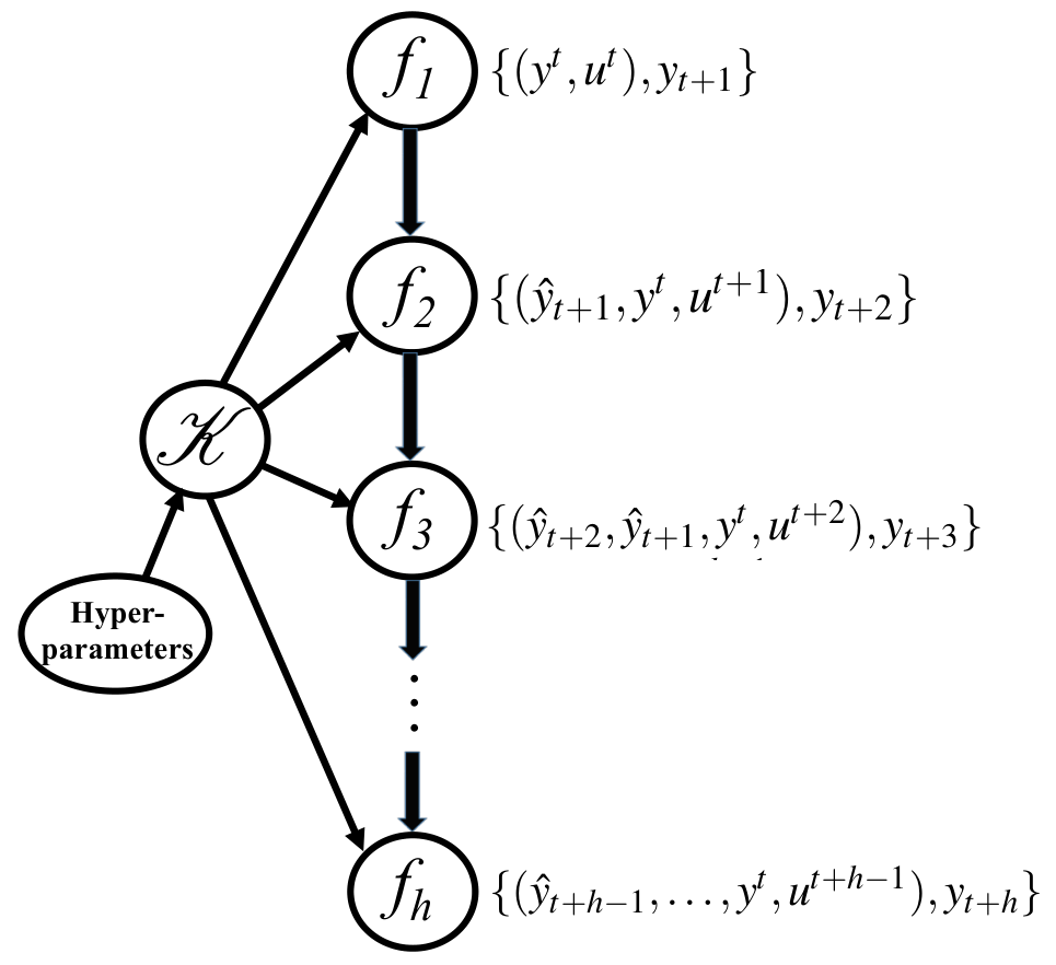 |
An application of a deep prediction network is illustrated in Fig. 10. It shows that the performance of the kernel-based estimator (53), used to obtain long-term predictions via (13), can be much improved when plugged in the new computational architecture.
5.6 Building compositional kernels using limits of deep neural networks
Kernels can be defined by a deep neural network by placing priors on its weights and letting its width (number of hidden units) grow to infinity. This construction also includes the connection with Gaussian regression obtained by Neal in [222] and mentioned at the beginning of the section. Recalling (10), any layer of a fully connected neural network is defined by an activation function , weight matrices and bias vectors . We model all the entries of and as independent and zero-mean random variables with variances
where is the width of the -th layer. Consider just a -layer structure whose output vector is where we use to denote the pre-activation signals in the -th layer, i.e.,
| (64a) | ||||
| (64b) | ||||
Any component is the sum of independent random variables. Hence, if the layer’s width approaches infinity, all will converge to Gaussian processes according to the multivariate central limit theorem. They turn also out mutually independent, allowing to iterate this argument making the hidden layer widths go to infinite in succession [93, 179]. In particular, any component of the output from the layer will be a zero-mean Gaussian process with covariance (kernel) functions given by:
| (65) | ||||
The advantage of this construction is that the resulting kernel may inherit some features of deep networks which can be implemented through convex estimators like kernel ridge regression (53). For ReLU activations, a closed-form expression is available and the result is the arccosine kernel originally derived in [82]:
with
Interestingly, this kernel has distinct features compared e.g. with the Gaussian and polynomial kernels described in (50) and (52), respectively. In fact, it favors nonnegative and sparse data representations, see [82] for more details.
A numerical example that illustrates the convergence of a DNN to a Gaussian process is given in Fig. 11 (left panel). In the infinite wide limit, we have seen that the function is a Gaussian process with a kernel derived from (65). Let denote the stacked observed inputs while is a test point. The function , evaluated on these points, becomes the following Gaussian random vector:
| (66) |
where we used to denote an matrix with entry . Similarly, notations like indicate the cross-covariance matrix between and that corresponds to sampled on . Using standard Gaussian conditioning formulas, we can compute the value at the test point conditioned on the observations , i.e.
where:
| (67a) | ||||
| (67b) | ||||
In Fig. 11 (left) we compare estimates from a neural network
of large width (and only with the last layer trained)
and from Gaussian regression with covariance defined by the same network
with the width growing to infinity.
They turn out quite similar.
As final remarks, the idea that infinitely wide neural networks can be seen as Gaussian Processes generalizes to convolutional neural networks [227] and to recurrent neural networks [346]. There are also formulations that try to generalize to a combination of any of these architectures in systematic ways [226, 346] and obtain the corresponding kernel from its specification. Other kernels inspired by deep structures can be found in [89, 101, 63] in the setting of the so-called deep Gaussian processes.
6 Theoretical development
The empirical success of deep learning methods brings to light the question of what makes these models so successful. Deep neural networks make little explicit effort to control model complexity and often have millions or, even, billions of parameters [317]. While the number of parameters is not always a good measure of the model capacity, deep learning models have been shown to have enough capacity to fit a training set labeled at random [356] and are therefore interpolators. It has also been observed that these models in some cases seem to indefinitely display increased performance as the model size increases [317]. We adopt the terminology of describing models with more parameters than training data points as overparameterized.
Inspired by Bartlett et al. [32], we would like to highlight two major research developments that have received attention from a theoretical perspective after surprising empirical observations made by practitioners using deep learning. The first studies the role of overparameterization simplifying the non-convex optimization problem that arises when training neural network to a more tractable optimization problem. The second development concerns the interplay between overparametrization and generalization: traditional system identification (and statistical) ideas suggest that flexible models with too many parameters will fit training data too well (up to interpolating the training data). These flexible models should learn spurious components of the data such as noise and provide poor predictive accuracy in new datasets as a consequence. However, there are significant cases where deep learning appears to contradict this accepted statistical wisdom since it performs well on unseen data even when almost perfect fitting to training data is obtained.
This section is structured as follows: in Section 6.1 we highlight the recent developments in the understanding of infinitely wide neural networks, explaining how non-convex optimization problems become more tractable as more parameters are used. We then illustrate the idea of implicit regularization (Section 6.2), showing how some optimization choices adopted in deep learning might be responsible for selecting solutions with desirable properties. In Section 6.3 we discuss the generalization of models that are overparameterized and perfectly interpolate training data. Section 6.4 introduces a simple numerical experiment in the linear setting where overparameterized models perform worse, which highlights that there are examples where overparameterization can be harmful. Finally, Section 6.5 describes some recent results on approximation capabilities of deep neural networks anticipated at the end of Section 2.
6.1 Infinitely-wide neural networks
In the limit, when a neural network grows infinitely wide the optimization problem for training becomes convex in an infinite dimensional space [9, 79, 99, 151]. – Here wide infinitely many nodes in one hidden layer opposed to deep neural networks with many layers. The idea can be understood in simple terms: Let the parametrized function denote the neural network and be the vector of parameters. Assume that the number of parameters is very large and that training the neural network changes each parameter just by a small amount w.r.t. its initialization during every update step. A linearization of the model around yields
| (68) |
where . Hence, the problem can be approximated by an affine problem that could be solved using linear regression. Indeed, it can be established that as the neural network become infinitely wide, the training of the neural network actually amounts to solving a problem similar to that in (68).
The notion can be formalized by considering the kernel that corresponds to the transformation , i.e.
| (69) |
which for a fixed is a positive-semidefinite kernel as defined in Eq. (44). The term neural tangent kernel was coined in [151] for this kernel since it describes the evolution of the neural networks during their training by gradient descent. Assume that the parameters are continuously updated in the negative direction of the gradient
| (70) |
This type of update is sometimes called gradient flow and is a continuous version of the gradient descent method. Here can be seen as the learning rate of the algorithm. A simple application of the chain rule reveals that
| (71) |
There are two challenges that make it difficult to apply traditional analysis to the above problem. First, for neural networks the parameters are usually initialized at random. Hence, we can think of as a random variable, and the kernel is not deterministic. Second, the kernel depends on a parameter that is itself updated during training. Hence, is a kernel that evolves with the training itself.
Jacot et al. [151] present a method of analysis that avoids these two problems: in Theorem 1 of [151] it is shown that in probability, as the width of the neural network layers approach infinity, where is a deterministic kernel; Moreover, it shows that if is updated during training in the negative direction of the gradient, then uniformly on all the training paths, holds. For a fixed kernel , we have that (71) is a linear ordinary differential equation with no explicit dependence on . Indeed, if we denote ,
| (72) |
its solution is
| (73a) | ||||
| (73b) | ||||
| where we denote (for compactness) the kernel matrix built with the input locations collected in as . Moreover, as , we have that . Hence, in the limit: | ||||
| (73c) | ||||
Comparing Eq. (73) with (54) we see that the solution obtained by gradient flow is similar to the solution of kernel ridge regression with parameter . It does have some additional offset terms and that represent the predictions of the neural network at initialization.
As discussed in Section 5.6, in the infinite wide limit, the function is a Gaussian process with a kernel ,
| (74) |
Equation (73) is thus an affine transformation of a multivariate normal variable. Some standard manipulation of normal multivariate variables (see [184, Section 9.A, Corollary 9.2]) yields that is normally distributed for mean and variance:
| (75a) | ||||
| (75b) | ||||
In Fig. 11 (right) we compare such predictions with a neural network trained with gradient descent. Note that the mean prediction is the same as kernel ridge regression for the kernel , but the presence of randomness at the initialization yield additional terms to the covariance matrix. Similarly to the kernel in Eq. (65), the neural tangent kernel can be computed recursively as:
| (76) | ||||
where,
| (77) |
and is defined as in Eq. (65) and is the derivative of the activation function. Comparing Fig. 11 panel thus illustrates the difference between neural-network GP and the neural tangent kernel solution. The neural tangent kernel can be generalized to convolutional neural networks [20], recurrent neural networks [7] and has been formalized in a systematic way through a programming language description [347].
The idea that infinitely-wide limit neural network optimization can be convex illustrates how overparametrization can be a way to obtain a more tractable optimization problem. That said, there are studies showing that only the infinitely-wide regime is not enough to justify the good properties of neural networks [80]. Finite-dimensional neural networks are the solution to certain classes of Banach spaces other than RKHS: in [235, 236, 238], representer theorems are derived for Neural Networks with ReLU activation functions, showing they are solutions to data fitting in bounded variation spaces.
These works suggest that the analysis of neural networks in the infinite width limit might not be enough to understand its properties, it also points to limitations of restricting the function space to RKHS. In [237], they draw an analogy between smoothing-vs-adaptive splines and finite-vs-infinite ReLU neural network comparisons. Smoothing spline (that are kernel methods) have a hard time learning functions that are not spatially homogeneous, and adaptive splines are better at fitting functions with changes in the variation over spaces. The authors argue that similar differences hold for the neural network in the infinite-vs-finite case.
6.2 Implicit regularization
In the discussion that followed from Fig. 1, we have categorized neural networks as belonging to the “alternative approach” to system identification: that is, the model is searched for in a very rich space and the model complexity is controlled through regularization. The classification into this category comes with some nuance though. While regularization methods that include dropout, weight decay and similar are usually included in order to get the best performance, they are not strictly needed. Even without explicit regularization it is still possible to obtain reasonably well performing models. To study this behavior, effort has been put into studying the implicit regularization mechanisms that act in a neural network during its training.
A prime example of the implicit regularization through the problem formulation is the matrix completion or reconstruction problem studied in [128]. Here, we have a low-rank true matrix from which we only observe some entries yielding the partially observed matrix and we try to regress the full matrix including the non-observed entries
| (78) |
with the linear operator and following . Since the problem is overparameterized and has many global minima. Instead of directly optimizing this problem, we factorize with , which imposes a rank constraint and makes the problem non-convex. Here, we focus on the case of without rank constraint. We cannot expect the obtained solution to recover the true values or to generalise to unseen test data as we can set the unobserved values to any arbitrary number. When optimizing using gradient descent with small step size, we obtain in both formulations (with and without factorization) zero training error, which indicates that the model memorized the entries. The relative reconstruction error for unseen test data in the non-factorized formulation is equal to the fraction of non-observed entries. However, for the factorized formulation the reconstruction test error is surprisingly much lower. Hence, the gradient descent optimization found a specific solution, which generalizes better without any constraint on the problem but only by rewriting the problem formulation. It turns out that gradient descent will in this scenario implicitly induce a low nuclear norm. Hence, the optimization algorithm itself has a form of implicit regularization.
Extending this observation, [224] use neural networks with one hidden layer trained with SGD. The authors observe that despite increasing the capacity, i.e. the number of hidden units, to and beyond the point where the model fits training data perfectly, generalization to unseen data is not harmed. This indicates that the capacity of the model is not controlled by the number of model parameters when trained with SGD and hints further to a regularizing behavior of gradient descent converging to a minimum norm solution.
The solution that is found in the matrix completion problem is for small step sizes in fact the minimum norm solution. Similarly, for overparameterized linear regression let us assume the cost function and the parameter update with gradient descent. Then if the initial parameter lies in the row space of and for a sufficiently small , we have that the solution converges to the minimum-norm solution, i.e. the solution to the following optimization problem
| (79) |
Barrett and Dherin tries to quantify the implicit regularization for gradient descent [30] which is extended in [306] for stochastic gradient descent with shuffling of the mini-batches. Due to the step-based nature of the algorithm, the optimization does not follow the continuous path of the gradient flow at each step exactly but follows a different trajectory of a modified cost including an implicit regularizer. Assume the same cost function and parameter update as for linear regression above with . Then gradient descent follows more closely with
| (80) | ||||
| with |
where is the gradient in the th direction. Hence, this formulation shows that gradient descent penalize directions with large cost. This penalization implies that gradient descent is biased towards flat minima, i.e. minima where the magnitude of the eigenvalues in are small, which the authors observe empirically. It is observed that that optimization solutions in sharp minima, i.e. with large Hessian, generalize less well. To make this more intuitive, assume that the test cost function is shifted w.r.t. the model parameters compared to the train cost function e.g. due to a change within the datasets. Hence, the obtained solution in the train minimum does not lie in the test minimum. When we found a solution in a sharp minimum this yields a large increase in test cost while a solution in a flat minimum does not yield such a large increase in test cost.
Keskar et al. provide evidence that optimizing with smaller batch sizes yields flat minima solutions [162]. The origin of this can be the stochasticity of smaller batch sizes. Pesme et al. [246] analyse the effect of stochasticity on the dynamics of SGD in the squared parameterization linear regression model [343], also known as diagonal linear network (meaning linear activation functions and diagonal weight matrices). The authors show that training with SGD always generalizes better than with gradient descent. The role of noise in the outputs or labels during training is analysed by [50, 132] which show that this stochasticity enforces sparse solution with minimum norm. The effect of the step size (or learning rate) is similar with larger step sizes leading to sharper minima [219].
6.3 Interpolation and double-descent curves
The generalization properties of deep neural networks motivate the study of models that can (almost) perfectly fit the training dataset. This is also noted as interpolation of training data. Indeed, Zhang et al. [356] showed that state-of-the-art deep architectures are sufficiently complex that they can be trained to interpolate noisy data. In a series of insightful papers Belkin et al. [40, 39, 41] illustrate that interpolation does not contradict good generalization. In [40] the authors coined the term double-descent curve for describing the curve of the model performance vs the number of parameters. The idea is that a “double-descent” curve subsumes the textbook U-shaped bias–variance trade-off curve in some scenarios with a second decrease in the error occurring beyond the point where the model has reached the capacity of interpolating the training data.
Double descent curve
Fig. 12 describes the double-descent phenomenon in an example adapted from [278]. The leftmost plot illustrates the one-step-ahead mean square error in training and test as a function of the number of parameters. A double descent curve can be observed in the test error. When , i.e. when the number of parameters is smaller than the dataset size, we can observe a U-shape error curve in the hold-out test set as we vary . However, as the number of parameters keeps increasing, it is possible to reach a point where the model starts to interpolate (usually at ) and the training error reaches zero. At this point, the model does not generalise well and will perform poorly on the unseen test dataset. However, if we continue to increase the number of parameters to , the model is overparameterized and will eventually start to generalise well again on test data.
One important element of the example is that in the overparameterized or interpolation region there are infinitely many solutions and we select the minimum-norm solution i.e. (79). In Section 2, we described cases where the number of data-points is larger than the dimension of the features vector and explained how in this setup sometimes the number of parameters can be used as a proxy for model complexity, e.g. as in (8). This does not apply for the case and indeed increasing the number of features can have the reverse effect. The middle plot in Fig. 12 illustrates that as the number of parameters increases it yields solutions with smaller parameter norm. The rightmost plot in Fig. 12 illustrates the one-step-ahead mean square error in the test set as a function of the parameter norm . This plot does not show a double descent but more a classical U-Shaped bias-variance trade-off. It highlights that the lowest test risk is not obtained in a second descent but rather at a sweet-spot in this U-Shaped curve defined by an intermediate value of the parameter norm.
The double-descent performance curve has been experimentally observed in diverse machine learning settings: Belkin et al. [40] show the phenomenon for random Fourier features, random forest and shallow networks, [134] for ridgeless regression, [220] for transformers and convolutional network models. Setups closed to the system identification are discussed in [278].
For completeness, we point out that in some cases it is possible to observe more than two descents in the generalization curve. To cite a few examples where this is demonstrated: Ascoli et al. [90] empirically showed the triple-descent phenomena to random Fourier model (same model used to produce Fig. 12 under different conditions) and [3] show it for the neural tangent kernel. Moreover, [70] illustrates a case with Gaussian mixtures, for which it is possible to obtain arbitrary many descents when the number of parameters increases and the number of training samples is kept constant.
Theoretical toolboxes
Many of the traditional asymptotic results in system identification assume that the number of parameters is fixed and that the number of data points goes to infinity . As we become interested in models where the number of parameters scales with data, different types of results are needed. We mention two interesting sets of tools that can be used to derive theoretical models of the above phenomenon. In describing them, recall that as a proxy for model capacity the number of data features, i.e. covariates in the data, is often considered instead of the number of model parameters. In a single layer model these two measures coincide. Hence, to be compliant with literature which often considers the number of features, we abuse notation and denote both by .
The first are high-dimensional asymptotic results. They consider the number of features and the number of data points and make them jointly grow to infinity, i.e. in such way that where is a fixed fraction. For example, random matrix theory has asymptotic results for the eigenvalues, eigenvectors and other properties of matrices with random entries [12, 26, 318]. The framework and potential of such theory, for explaining and studying neural networks when and tend to infinity, have been the focus of recent work, see e.g. [240, 244, 245] and also Fig. 13 where one result is illustrated. Random matrix theory has also been a powerful tool in generating theoretical models for the double-descent phenomenon [4, 3, 39, 134, 210].
Another powerful set of tools are non-asymptotic bounds. Indeed, the benign overfitting phenomenon (described later on) is derived in [33] using such bounds. In this case, the number of parameters and data points are considered as fixed to finite values. High-probability statements are then derived as a function of them. In the last decade the study of concentration inequalities has gone through significant developments due to its application in high-dimensional statistics and signal processing, see the textbooks [332, 338] for a comprehensive cover this topic. We also mention that these areas are all closely related: tail bounds and concentration inequalities typically underlie the proofs of classical asymptotic theorems.
Asymptotic models of double-descent
As one simple example of asymptotic analysis, we highlight results from [134]. Consider a simple linear regression problem where training and test data have been generated linearly with additive noise:
| (81) |
In (81), is a distribution in such that and . is a distribution in which implies . Moreover, and . The and the are all mutually independent. The norm of the data generation parameter is denoted by .
Now, assume that has been estimated using the minimum-norm solution: , where denotes the pseudoinverse, we obtain that:
| (82) |
The first term can be understood as the projection of the true parameter that generated the data in the row space of . The second term is related to how much the model learns from the noise.
When , the eigenvalues of converge to the Marchenko–Pastur distribution, see the leftmost plot in Fig. 13. This fact is used in [134] to obtain asymptotics concerning the error in new data points as well as the parameter norm of the estimated parameters. Specifically, as with , almost surely
| (83) | |||||
| (84) |
This example is illustrated in the middle plot of Fig. 13. While simple and displaying a double-descent behavior, this is a theoretical model for which the performance in the underparametrized region is still better than the one in the overparameterized region.
The right panel of Fig. 13 shows one example also from [134] where the covariance matrix of has a spiked structure: the first eigenvalues have high value while the remaining ones are small and correspond mostly to error in variables components. As discussed in the next subsection, the profile of the eigenvalues of the data covariance matrix plays an important role for obtaining good performance in the overparameterized region. Usually, having some more important components and a sufficiently fast decay of the other ones is related to it.
Asymptotic results for more realistic scenarios have also been derived. For instance, Mei and Montanari [210] derive asymptotics for the random features model. It is actually described as:
| (85) |
where the matrix is initialized from a random distribution and only the parameter is trained. This is the model used for estimating the nonlinear ARX model in Fig. 12 and can be understood as a neural network where only the last layer is trained.
Benign overfitting
Bartlett et al. [33] coined the term “benign overfitting”. Overfitting describes phenomena where models fit noisy data too well. Most classical texts on statistics and machine learning associate to these situations poor generalization. The viewpoint has become so prevalent that the word ‘overfitting’ is often taken to mean both fitting data better than should be expected and also giving poor predictive accuracy as a consequence. In [33], the term is used in the literal meaning of the word ‘overfitting’. Next, conditions under which this overfitting is not necessarily harmful for model performance are obtained.
Indeed Bartlett et al. [33] provide a finite sample characterization of the error in linear regression problems and establish conditions for benign overfitting to occur. They show that the eigenvalues of the data covariance play a crucial role in the characterization of benign overfitting and need to decay with certain rates. The covariates must lie in some dominant directions corresponding to large eigenvalues while still have small components (and hence unimportant) along directions in parameter space where the label noise can be hidden. Mallinar et al. [205] extend the taxonomy of overfitting from benign and catastrophic to ‘tempered’. The authors argue that many interpolators such as DNNs do neither overfit benignly nor catastrophically.
6.4 The risk of overfitting in linear system identification
Studies on overparametrization like [32, 183] include conditions such that the “simplest” (minimum norm) function that interpolates the identification data may generalize well on new outputs. However, results mainly concern predictions of future data which follow the same distributions of the training data. This can be a drawback in control where one often wants robustness e.g. with respect of significant variations in the system input and of disturbances. In this regard, carefully-tuned regularization can largely outperform the implicit regularization obtained by the pseudo-inverse since it can encode useful information about the system. This is now illustrated in a linear setting using the kernel-based regularization described in Section 5.
Different discrete-time stable impulse responses are obtained by converting in discrete-time random rational transfer functions of order 30 obtained by the MATLAB command rss. In particular, the continuous-time function returned by this routine is truncated over the finite interval , with such as to capture of its two-norm. The impulse response is then uniformly sampled to obtain a vector containing impulse response coefficients. Our measurements model is
| (86) |
where are realizations of independent uniform random variables over . The form a white Gaussian noise, independent of , and the signal-to-noise ratio is 100. Estimation of from is ill-posed and ill-conditioned since the measurements are obtained by discrete-time integrators. This is a situation frequently encountered in real applications where a dynamic system can be subject to a low-pass input.
The impulse response estimate is computed using regularized least squares (ReLS) (55) with regularization matrix defined by the stable spline/TC kernel (49) which provides information on smooth exponential decay. The strength of the regularizer is thus established by the regularization parameter and the decay rate .
Consider two versions of this estimator which differ in the adopted hyperparameters values. The first one, denoted by ReLS-TC, determines and via marginal likelihood (ML) optimization (58). The second estimator uses the ML estimate of but then computes the impulse response of minimum stable spline norm which interpolates the outputs, i.e. it computes
| (87) |
The resulting estimator is denoted by PI-TC where PI stays for Pseudo Inverse.
Given validation outputs , the prediction fit returned by a predictor is
| (88) |
where is the average value of the validation outputs. In our case, we have two predictors at stake, associated to ReLS-TC and PI-TC. In addition, we will consider two different validation sets of size 1000. The first one contains outputs generated as in (86) but without adding noise and generating other independent realizations of . So, the first validation set is still connected with a low-pass (LP) input. The second one contains 1000 noiseless outputs from the FIR with coefficients in with white Gaussian noise (WN) as input.
Results from a Monte Carlo experiment of 100 runs are in Fig. 14 where Matlab boxplots of the 100 prediction fits returned by the two estimators are displayed. Using the first validation set (top), ReLS-TC provides the best results but the prediction performance of PI-TC is comparable. This means that the stable spline pseudo-inverse may well generalize on new data which are still integral versions of the impulse responses. The picture changes completely by considering validation data generated using as input. Using the second test set (bottom) one can see that carefully tuned regularization in many cases generalize well also when future data follow statistics much different from those underlying the training set.
6.5 Approximation properties of deep neural networks
Some recent studies on deep network properties in approximating input-output maps are now briefly discussed. They support the use of these networks to face the curse of dimensionality in regression problems.
Consider the fully connected neural network with one hidden layer given by (10) with null . It is composed of units (basis functions) that receive the vector as input and return as output the scalar
| (89) |
Consider now the following approximation problem. A smooth map over a compact set of and a resolution are given. Then, the network has to adjust weight vectors and scalars to synthesize such that
| (90) |
It turns out e.g. from [31, 212, 259, 260] that this goal can always be achieved by the shallow network (89) which is therefore universal. However, the number of required trainable parameters is , hence the network’s complexity scales exponentially with the required accuracy11 1 More specifically, this and the next result here discussed hold by choosing infinitely differentiable and different from a polynomial. Furthermore, the sup-norm of and of its first-order partial derivatives are assumed bounded over its compact domain.. This is the best possible result [96] unless additional information on is provided.
As the intuition suggests, a situation where a deep network can significantly improve this outcome is when has a compositional structure. As an example, could be defined by local functions of only two variables, e.g. when has only 8 components , we have
| (91) | ||||
where each function is implemented via a node of the network through a certain number of units. It turns out that a deep network, given by a simple binary tree with three layers if (91) holds, achieves the same resolution as the shallow network but with a different number of parameters, . Such results extend to other hierarchical functions and the complexity depends on the (possibly different) number of edges entering the nodes [260, Section 4]. Hence, shallow and deep networks are both universal approximators (they can approximate any reasonable continuous function arbitrarily well). However, by knowing the compositional structure the challenging curse of dimensionality can sometimes be handled by reducing the number of model parameters from exponential to linear in the dimension of the function domain.
Other studies that support deep networks for regression are found in [91, 321]. Consider the function
induced by a deep network which adopts the ReLU . Each unit thus returns the piecewise linear function with breakpoint established by . This makes also the overall function piece-wise linear being formed by linear operations mixed with the max function. So, the flexibility of this network can be measured by how many breakpoints can be introduced in the curve . Such concept has some limitations since there can be hidden correlations between the breakpoints induced by the model. However, focusing mostly on the case of scalar inputs () and outputs, results in [91, 321] and simulations based on random networks in [192, Section 6] suggest that, while the number of breakpoints grows quickly with the depth of the network, the number of parameters does not increase with the same rate. This means that increasing the number of layers is more effective than increasing the number of units per layer. For very special selections of weights and biases, the maximum number of breakpoints scales as if all the hidden layers have the same width (number of units) . It is also proved that deep ReLU networks reach the same approximation power of free knot linear splines with a comparable number of parameters, but can also generate other functions distant from them. Advantages of deep learning for other classes, like power and Lipschitz functions, are discussed in [348, 349].
7 Applications
7.1 Software issues
Deep neural networks have been used extensively and a substantial amount of software has been developed in different contexts and for different platforms. Python implementations, like PyTorch22 2 https://pytorch.org/ [241], TensorFlow33 3 https://www.tensorflow.org/ [1] and JaX44 4 https://github.com/google/jax [60] are quite popular and are open source libraries. In this survey we focus on Matlab and PyTorch.
MATLAB is a proprietary programming and numeric computing platform. Matlab has a Deep Learning Toolbox (DLT) which implements most of the deep networks for various applications, described in this paper. Of particular interest for system identification is how the DLT cooperates with the System Identification Toolbox (SITB) [191] to identify systems using deep learning. SITB has a model object idnlarx that implements nonlinear models of ARX-character
| (92) |
where is a vector of a finite number of past inputs and outputs while is a nonlinear function that can be defined in many different ways. If NET is a shallow or deep neural network defined in DLT, a nlarx model can be defined by
Ψmn = idFeedforwardNetwork(NET)
Ψ
The object mn is now a regular SITB model that can be estimated and evaluated by any SITB command, e.g.
Ψmhat = nlarx(Data,[2 2 1],mn)
Ψcompare(Data,mhat);
Ψys = sim(mhat,newdata);
Ψresid(Data,mhat)
Ψ
PyTorch is an open-source framework implemented in Python. The framework provides the basic components for the implementation and training of neural networks and it is widely used in the machine learning community and is the basis of many state-of-the-art applications. There is no specific system identification package, but the building blocks provided allow for the facilitated implementation of all the models described in this paper. For instance, a fully connected network with one hidden layer would be implemented as:
Ψclass FCNetwork(nn.Module):
Ψdef __init__(self, n_inputs, n_hidden):
Ψsuper(FCNetwork, self).__init__()
Ψself.net = nn.Sequential(
Ψ[
Ψnn.Linear(n_inputs, n_hidden),
Ψnn.ReLU(),
Ψnn.Linear(n_hidden, 1)
Ψ])
Ψ
Ψdef forward(self, x):
Ψreturn self.net(x)
Ψ
The package provides:
- 1.
GPU acceleration capabilities. The acceleration is obtained with few lines of code and can make the neural network implementation and training significantly faster, e.g.,
ΨΨmodel = FCNetwork() ΨΨdevice = torch.device("cuda") ΨΨmodel.to(device=device) ΨΨ - 2.
Automatic differentiation capabilities, that allow the derivatives of the neural network to be easily computed and gradient-descent-based optimization to be used to update the model. For instance, one step of an stochastic gradient descent could be computed as:
ΨΨmodel_output = model(x)
ΨΨloss = loss_function(model_output, y)
ΨΨloss.backward()
ΨΨoptimizer.step()
ΨΨ
7.2 An example with real data: forced duffing oscillator
The system is an electronic circuit that mimics a nonlinear mechanical system with a cubic hardening spring. This class of nonlinear systems has a very rich behavior, including regular and chaotic motions, and the generation of sub-harmonics. The dataset55 5 Data are available at www.nonlinearbenchmark.org/#Silverbox. The selection of estimation and validation data is the same as in Listing S1 in [299].has often been used in nonlinear identification benchmarks, also to test deep networks, see e.g. [192, 299].
Two sets of data were collected with different excitations, depicted in Fig. 15.
The estimation data are used to fit a model. Then, following what was illustrated in Section 2, the model’s validity is checked by how well it reproduces the validation data according to (4). That is, the model is simulated using the validation data input and the discrepancy between model output and measured validation data output is determined.
Linear Model
A common linear model of the Box-Jenkins type (see e.g. Chapter 4 in [190]) with 4 poles, 4 zeros and a second order noise transfer function, is estimated by
Ψmbj=bj(edat,[4 4 2 2 0]);
Ψ
The accuracy of this model is computed by
Ψ[ys,Fit]=compare(vdat,mbj)
ΨFit=29.71 % (percent of the output variation ...
Ψreproduced by the model)
Ψ
with the Fit defined as in (88). The validation output and the error between this and the simulated model output is shown in Fig. 16. It can be seen that the simulation is not very good. The error is at times as big as the signal itself.
Residual analysis as mentioned in Section 2.2 can also be performed by the command resid(vdata,mbj). It shows that there is quite significant correlation between the residuals and the input. The model should thus be rejected.
Deep Cascaded Network
A deep learning model with 6 layers of feedforward nets (cf Sec. 3.2) with 6 nodes each is estimated and validated by
Ψnet=cascadeforwardnet([6,6,6,6,6,6]);
ΨN2=idFeedforwardNetwork(net);
ΨmN2=nlarx(edat,[4 4 0],N2);
Ψ[Ys,Fit]=compare(vdat,mN2)
ΨFit=99.18
Ψ
The validation output and the error between this and the simulated model output is shown in Fig. 17. The simulation is remarkably good: the error is hardly visible. Recall that the simulation is done without any access to the measured validation output, and note that the character of the validation data is quite different from that of the estimation data.

The residual analysis (resid(vdata,mN2)) for this model is shown in Fig. 18. The correlation between the residuals and past inputs (lag larger than 0) in the right panel is quite insignificant. There is some correlation left among the (very small) residuals themselves (left panel) but no attempt has been made to build a model for the color of the additive disturbances.

7.3 PyTorch example: coupled electronic drives
In this example we will make use of PyTorch code to implement deep neural networks to model an open nonlinear system identification benchmark. The underlying physical system consists of two electrical motors which are connected to a pulley through a flexible belt [342]. Two different input signals are available66 6 The complete dataset and dataset descriptions are available at https://www.nonlinearbenchmark.org/benchmarks/coupled-electric-drives.: a pseudo-random binary sequence and a uniformly distributed input signal. We use the uniformly distributed input signal to learn the dynamics using 60% of the data and validate it on the remaining 40%. This nonlinear dataset was used in previous studies [139, 163] and can be modeled by a Wiener-Hammerstein model [342].
We compare four models; 1) a fully connected (FC) neural network, see Section 3.1, with three layers and 300 hidden units; 2) an LSTM, see Section 3.4 with one layer and 200 hidden units; 3) a deep state-space model (SSM), see Section 3.5, specifically a VAE-RNN from [110, 118] with one layer for all representations, a hidden size of 100 for the deterministic latent variable and 50 for the stochastic one; and 4) a baseline linear ARX model for comparison. We train all the deep models using stochastic gradient descent with momentum for 100 (FC) or 150 (LSTM and Deep SSM) epochs. The baseline ARX model was trained using the least squares solution. For all models we use an input and output memory of 5, see (12), which was the one that gave the best results by grid search for the feedforward neural network model. As a comparison, the reference model provided in [342] is a continuous system of third order.
We evaluate the models using the 40% hold-out validation dataset. In Fig. 19, we compared the measured validation output with the simulated response from some of the models. We compute the fit as defined in (88) to the validation data as well as to the training data. The same metric is used internally in the function compare in MatLab to provide the fit. In Fig. 20 we show the fit of the simulated response, the boxplot is displayed for 25 different initializations of each architecture.77 7 For the linear model there is no stochasticity because of the global least square solution.
The results indicate that the deep models show a good performance in comparison to the linear baseline model. This is especially noteworthy as we use 300 time samples for training while our models have (FC), (LSTM) and (deep SSM) parameters. Hence, despite the fact that the models are overparameterized, they generalize quite well on validation data, which is in accordance with the theoretical discussions in Sections 6.2 and 6.3.
8 Conclusions
Inferring models of dynamical systems from observed input-output data is the aim of System Identification. We have demonstrated in this survey that sophisticated modern deep learning techniques also share the essential features of this problem. Deep (neural) networks, as e.g. described in Section 3, can in fact serve as model structures producing predictions of future observations that can be fitted to observed data, just as in the conventional prediction error approach. Analogously, concatenated kernels can define new regularized methods, as the estimator (61) described in Section 5.
What is essential in these deep estimation techniques is (a) that they employ (very) many parameters and (b) that the parameterizations can be made in various compositions, exploiting repeated structures (layers) and other concatenations, as in the simple illustrative example (91). This motivates the concept of deep structures.
The large size of the parameter vector calls for special attention, methods, and “tricks” in the numerical and algorithmic treatments, as detailed in Section 4. The overparameterized case (more parameters than observations) also gives rise to model behavior that apparently defies statistical truths: ”generalization behavior too good to be true”, as illustrated in Section 6.3.
In this way, deep learning is not just “a special case of system identification” and the survey has shown a rich set of issues and techniques that could be useful for expanding the understanding of this fundamental control area. This can be pursued by focusing on several interesting open problems. For instance, while Section 3 presented common deep architectures and how they have been adapted for system identification, there is also a range of modern architectures which have been successful in other tasks but still not extensively used for nonlinear system identification. They include:
- •
- •
- •
- •
Regarding overparametrization, Section 6.3 described both experimental and theoretical results for double-descent. But studies have so far focused on static systems: the challenge is to derive (asymptotic or finite-sample) theoretical models for data generated by dynamic equations. Finally, robustness issues, as the building of uncertainty bounds around deep models of dynamic systems, can also play an important role in many future control applications.
References
- [1] M. Abadi, P. Barham, J. Chen, Z. Chen, A. Davis, J. Dean, M. Devin, S. Ghemawat, G. Irving, M. Isard, et al. TensorFlow: A system for large-scale machine learning. In 12th USENIX symposium on operating systems design and implementation (OSDI 16), pages 265–283, 2016.
- [2] A. Abbas, D. Sutter, A. Figalli, and S. Woerner. Effective dimension of machine learning models. arXiv: 2112.04807, 2021.
- [3] B. Adlam and J. Pennington. The Neural Tangent Kernel in High Dimensions: Triple Descent and a Multi-Scale Theory of Generalization. Proceedings of the 37 th International Conference on Machine Learning, PMLR 119, 2020.
- [4] M.S. Advani, A.M. Saxe, and H. Sompolinsky. High-dimensional dynamics of generalization error in neural networks. Neural Networks, 132:428–446, December 2020.
- [5] L.A. Aguirre, B. Barbosa, and A.P. Braga. Prediction and simulation errors in parameter estimation for nonlinear systems. Mechanical Systems and Signal Processing, 24(8):2855–2867, 2010.
- [6] H. Akaike. A new look at the statistical model identification. IEEE Transactions on Automatic Control, AC-19:716–723, 1974.
- [7] S. Alemohammad, Z. Wang, R. Balestriero, and R. Baraniuk. The recurrent neural tangent kernel. In International conference on learning representations, 2021.
- [8] A. Alessandri, M. Baglietto, and G. Battistelli. Moving-horizon state estimation for nonlinear discrete-time systems: New stability results and approximation schemes. 44(7):1753–1765, 2008.
- [9] Z. Allen-Zhu, Y. Li, and Z. Song. A Convergence Theory for Deep Learning via Over-Parameterization. Proceedings of the 36 th International Conference on Machine Learning, PMLR, 97, 2019.
- [10] J. An and S. Cho. Variational autoencoder based anomaly detection using reconstruction probability. Special Lecture on IE, 2:1–18, 2015.
- [11] B.D.O. Anderson and J.B. Moore. Optimal Filtering. Prentice-Hall, Englewood Cliffs, N.J., USA, 1979.
- [12] G.W. Anderson, A. Guionnet, and O. Zeitouni. An Introduction to Random Matrices. 2009.
- [13] C. Andersson, A.H. Ribeiro, K. Tiels, N. Wahlström, and T.B. Schön. Deep Convolutional Networks in System Identification. Proceedings of the 58th IEEE Conference on Decision and Control (CDC), pages 3670–3676, September 2019.
- [14] D. Angeli. A Lyapunov approach to incremental stability properties. IEEE Transactions on Automatic Control, 47(3):410–421, 2002.
- [15] A. Aravkin, B.M. Bell, J.V. Burke, and G. Pillonetto. The connection between Bayesian estimation of a Gaussian random field and RKHS. IEEE Transactions on Neural Networks and Learning Systems, 26(7):1518–1524, 2015.
- [16] A. Aravkin, J.V. Burke, A. Chiuso, and G. Pillonetto. Convex vs non-convex estimators for regression and sparse estimation: the mean squared error properties of ard and glasso. The Journal of Machine Learning Research, 15(1):217–252, 2014.
- [17] A. Aravkin and D. Davis. Trimmed statistical estimation via variance reduction. Mathematics of Operations Research, 45(1):292–322, 2020.
- [18] A. Argyriou and F. Dinuzzo. A unifying view of representer theorems. In Proceedings of the 31th International Conference on Machine Learning, volume 32, pages 748–756, 2014.
- [19] N. Aronszajn. Theory of reproducing kernels. Trans. of the American Mathematical Society, 68:337–404, 1950.
- [20] S. Arora, S. Du, W. Hu, Z. Li, R. Salakhutdinov, and R. Wang. On exact computation with an infinitely wide neural net. In Thirty-third conference on neural information processing systems, 2019.
- [21] K. Astrom and T. Bohlin. Numerical identification of linear dynamic systems from normal operating records. In Proc. of IFAC Symposium on self-adaptive control systems, 1965.
- [22] A. Azulay and Y. Weiss. Why do deep convolutional networks generalize so poorly to small image transformations? Journal of Machine Learning Research, 20:1–25, 2019.
- [23] D. Bahdanau, K. Cho, and Y. Bengio. Neural machine translation by jointly learning to align and translate. arXiv:1409.0473, 2014.
- [24] E.W. Bai, C. Cheng, and W.X. Zhao. Variable selection of high-dimensional non-parametric nonlinear systems by derivative averaging to avoid the curse of dimensionality. Automatica, 101:138 – 149, 2019.
- [25] S. Bai, J.Z. Kolter, and V. Koltun. An Empirical Evaluation of Generic Convolutional and Recurrent Networks for Sequence Modeling. arXiv:1803.01271, 2018.
- [26] Z. Bai and J.W. Silverstein. Spectral analysis of large dimensional random matrices, volume 20 of Springer Series in Statistics. Springer, 2010.
- [27] B. Bakker and T. Heskes. Task clustering and gating for Bayesian multi-task learning. Journal of Machine Learning Research, (4):83–99, 2003.
- [28] P. Baldi and K. Hornik. Neural networks and principal component analysis: learning from examples without local minima. Neural Networks, 2:53–58, 1989.
- [29] N.E. Barabanov and D.V. Prokhorov. Stability analysis of discrete-time recurrent neural networks. IEEE Transactions on Neural Networks, 13(2):292–303, 2002.
- [30] D. Barrett and B. Dherin. Implicit gradient regularization. In International Conference on Learning Representations, 2021.
- [31] A.R. Barron. Universal approximation bounds for superposition of a sigmoidal function. IEEE Trans. on Information Theory, 39:930–945, 1993.
- [32] Peter L Bartlett, Andrea Montanari, and Alexander Rakhlin. Deep learning: a statistical viewpoint. Acta numerica, 30:87–201, 2021.
- [33] P.L. Bartlett, P.M. Long, G. Lugosi, and A. Tsigler. Benign overfitting in linear regression. Proceedings of the National Academy of Sciences, 117(48):30063–30070, April 2020.
- [34] F. Bayer, M. Burger, and F. Allgöwer. Discrete-time incremental iss: A framework for robust nmpc. In 2013 European Control Conference (ECC), pages 2068–2073, 2013.
- [35] J. Bayer and C. Osendorfer. Learning stochastic recurrent networks. arXiv:1411.7610, 2014.
- [36] A. Beck. First-order methods in optimization. SIAM, 2017.
- [37] A. Beck and M. Teboulle. A fast iterative shrinkage-thresholding algorithm for linear inverse problems. SIAM journal on imaging sciences, 2(1):183–202, 2009.
- [38] G. Beintema, R. Toth, and M. Schoukens. Nonlinear state-space identification using deep encoder networks. In Learning for Dynamics and Control, pages 241–250. PMLR, 2021.
- [39] M. Belkin, D. Hsu, and J. Xu. Two Models of Double Descent for Weak Features. SIAM Journal on Mathematics of Data Science, 2(4):1167–1180, January 2020.
- [40] M. Belkin, S. Hsu, D.and Ma, and S. Mandal. Reconciling modern machine-learning practice and the classical bias–variance trade-off. Proceedings of the National Academy of Sciences, 116(32):15849–15854, August 2019.
- [41] M. Belkin, S. Ma, and S. Mandal. To understand deep learning we need to understand kernel learning. In Proceedings of the 35th International Conference on Machine Learning, volume 80 of Proceedings of Machine Learning Research, pages 541–549. PMLR, 10–15 Jul 2018.
- [42] Y. Bengio, A. Courville, and P. Vincent. Representation learning: A review and new perspectives. IEEE transactions on pattern analysis and machine intelligence, 35:1798–1828, 2013.
- [43] Y. Bengio, R. Ducharme, P. Vincent, and C. Jauvin. A neural probabilistic language model. Journal of Machine Learning Research, 3:1137–1155, 2003.
- [44] Y. Bengio, P. Simard, and P. Frasconi. Learning long-term dependencies with gradient descent is difficult. IEEE Transactions on Neural Networks, 5(2):157–166, March 1994.
- [45] S. Bergman. The Kernel Function and Conformal Mapping. Mathematical Surveys and Monographs, AMS, 1950.
- [46] M. Bertero. Linear inverse and ill-posed problems. Advances in Electronics and Electron Physics, 75:1–120, 1989.
- [47] G. Birpoutsoukis, A. Marconato, J. Lataire, and J. Schoukens. Regularized nonparametric Volterra kernel estimation. Automatica, 82:324 – 327, 2017.
- [48] C.M. Bishop. Pattern recognition and machine learning. Information science and statistics. Springer, New York, 2006.
- [49] M. Bisiacco and G. Pillonetto. On the mathematical foundations of stable RKHSs. Automatica, 2020.
- [50] G. Blanc, N. Gupta, G. Valiant, and P. Valiant. Implicit regularization for deep neural networks driven by an ornstein-uhlenbeck like process. In Proceedings of Thirty Third Conference on Learning Theory, volume 125 of Proceedings of Machine Learning Research, pages 483–513. PMLR, 2020.
- [51] D.M. Blei, A. Kucukelbir, and J.D. McAuliffe. Variational Inference: A Review for Statisticians. Journal of the American Statistical Association, 112(518):859–877, April 2017.
- [52] B. Bohn, C. Rieger, and M. Griebel. A representer theorem for deep kernel learning. Journal of Machine Learning Research, 20:1–32, 2019.
- [53] F. Bonassi, M. Farina, and R. Scattolini. On the stability properties of gated recurrent units neural networks. Systems and Control Letters, 157:105049, 2021.
- [54] F. Bonassi, M. Farina, and R. Scattolini. Stability of discrete-time feed-forward neural networks in NARX configuration. IFAC-PapersOnLine, 54(7):547–552, 2021. 19th IFAC Symposium on System Identification SYSID 2021.
- [55] F. Bonassi, C.F. Oliveira da Silva, and R. Scattolini. Nonlinear mpc for offset-free tracking of systems learned by gru neural networks. IFAC-PapersOnLine, 54(14):54–59, 2021. 3rd IFAC Conference on Modelling, Identification and Control of Nonlinear Systems MICNON 2021.
- [56] F. Bonassi, E. Terzi, M. Farina, and R. Scattolini. Lstm neural networks: Input to state stability and probabilistic safety verification. In Proceedings of the 2nd Conference on Learning for Dynamics and Control, volume 120 of Proceedings of Machine Learning Research, pages 85–94, 2020.
- [57] L. Bottou, F. E. Curtis, and J. Nocedal. Optimization methods for large-scale machine learning. SIAM Review, 60(2):223–311, 2018.
- [58] O. Bousquet and L. Bottou. The tradeoffs of large scale learning. pages 161–168, 2008.
- [59] S. Boyd and L. Chua. Fading memory and the problem of approximating nonlinear operators with volterra series. IEEE Transactions on Circuits and Systems, 32(11):1150–1161, 1985.
- [60] J. Bradbury, R. Frostig, P. Hawkins, M.J. Johnson, C. Leary, D. Maclaurin, G. Necula, A. Paszke, J. VanderPlas, S. Wanderman-Milne, and Q. Zhang. JAX: composable transformations of Python+NumPy programs, 2018.
- [61] M. Bronstein, J. Bruna, T. Cohen, and P. Veličković. Geometric deep learning: Grids, groups, graphs, geodesics, and gauges. arXiv:2104.13478, 2021.
- [62] L. Bugliari Armenio, E. Terzi, M. Farina, and R. Scattolini. Model predictive control design for dynamical systems learned by echo state networks. IEEE Control Systems Letters, 3(4):1044–1049, 2019.
- [63] T.D. Bui, J.M. Hernández-Lobato, D. Hernández-Lobato, Y. Li, and R.E. Turner. Deep gaussian processes for regression using approximate expectation propagation. In Proceedings of the 33rd International Conference on International Conference on Machine Learning - Volume 48, page 1472–1481, 2016.
- [64] R. Calandra, J. Peters, C. Rasmussen, and M.P. Deisenroth. Manifold gaussian processes for regression. In 2016 International Joint Conference on Neural Networks (IJCNN), pages 3338–3345, 2016.
- [65] D. Cao, Y. Wang, J. Duan, C. Zhang, X. Zhu, C. Huang, Y. Tong, B. Xu, J. Bai, J. Tong, et al. Spectral temporal graph neural network for multivariate time-series forecasting. Advances in Neural Information Processing Systems, 33:17766–17778, 2020.
- [66] W. Cao, V. Mirjalili, and S. Raschka. Rank consistent ordinal regression for neural networks with application to age estimation. Pattern Recognition Letters, 140:325–331, 2020.
- [67] R. Caruana. Multitask learning. Mach. Learn., 28(1):41–75, 1997.
- [68] S. Chandar, C. Sankar, E. Vorontsov, S.E. Kahou, and Y. Bengio. Towards Non-Saturating Recurrent Units for Modelling Long-Term Dependencies. Proceedings of the AAAI Conference on Artificial Intelligence, 33:3280–3287, July 2019.
- [69] V. Chandrasekaran, B. Recht, P.A. Parrilo, and A.S. Willsky. The convex geometry of linear inverse problems. Foundations of Computational Mathematics, 12(6):805–849, 2012.
- [70] L. Chen, Y. Min, M. Belkin, and A. Karbasi. Multiple Descent: Design Your Own Generalization Curve. In Advances in Neural Information Processing Systems, volume 34, pages 8898–8912, 2021.
- [71] R. Chen, Y. Rubanova, J. Bettencourt, and D.K. Duvenaud. Neural ordinary differential equations. Advances in neural information processing systems, 31, 2018.
- [72] S. Chen, S. A. Billings, and P. M. Grant. Nonlinear system identification using neural networks. International Journal of Control, 51(6):1191–1214, 1990.
- [73] T. Chen, M. S. Andersen, L. Ljung, A. Chiuso, and G. Pillonetto. System identification via sparse multiple kernel-based regularization using sequential convex optimization techniques. IEEE Transactions on Automatic Control, 59(11):2933–2945, 2014.
- [74] T. Chen, H. Ohlsson, and L. Ljung. On the estimation of transfer functions, regularizations and Gaussian processes - Revisited. Automatica, 48:1525–1535, 2012.
- [75] C.M. Cheng, Z.K. Peng, W.M. Zhang, and G. Meng. Volterra-series-based nonlinear system modeling and its engineering applications: A state-of-the-art review. Mechanical Systems and Signal Processing, 87:340 – 364, 2017.
- [76] Jen-Tzung Chien and Yuan-Chu Ku. Bayesian recurrent neural network for language modeling. IEEE transactions on neural networks and learning systems, 27:361–374, 2015.
- [77] M. Chilali and P. Gahinet. H-infinity design with pole placement constraints:an lmi approach. IEEE Transactions on Automatic Control, 41:358–367, 1996.
- [78] A. Chiuso. Regularization and Bayesian learning in dynamical systems: Past, present and future. Annual Reviews in Control, 41:24 – 38, 2016.
- [79] L. Chizat and F. Bach. On the global convergence of gradient descent for over-parameterized models using optimal transport. In Advances in neural information processing systems, volume 31, 2018.
- [80] L. Chizat, E. Oyallon, and F. Bach. On Lazy Training in Differentiable Programming. Advances in Neural Information Processing Systems 32, 2019.
- [81] K. Cho, B. van Merriënboer, C. Gulcehre, D. Bahdanau, F. Bougares, H. Schwenk, and Y. Bengio. Learning Phrase Representations using RNN Encoder–Decoder for Statistical Machine Translation. In Proceedings of the 2014 Conference on Empirical Methods in Natural Language Processing (EMNLP), pages 1724–1734, Doha, Qatar, October 2014. Association for Computational Linguistics.
- [82] Y. Cho and L. Saul. Kernel methods for deep learning. In Advances in Neural Information Processing Systems, volume 22, 2009.
- [83] K. Chua, R. Calandra, R. McAllister, and S. Levine. Deep reinforcement learning in a handful of trials using probabilistic dynamics models. In Deep reinforcement learning in a handful of trials using probabilistic dynamics models, 2018.
- [84] J. Chung, C. Gulcehre, K. Cho, and Y. Bengio. Empirical Evaluation of Gated Recurrent Neural Networks on Sequence Modeling. arXiv:1412.3555, December 2014.
- [85] J. Chung, K. Kastner, L. Dinh, K. Goel, A.C. Courville, and Y. Bengio. A recurrent latent variable model for sequential data. Advances in neural information processing systems, 28, 2015.
- [86] F. Cucker and S. Smale. On the mathematical foundations of learning. Bulletin of the American mathematical society, 39:1–49, 2001.
- [87] A. Dalla Libera, R. Carli, and G. Pillonetto. Kernel-based methods for Volterra series identification. Automatica, 129:109686, 2021.
- [88] A. Dalla Libera and G. Pillonetto. Deep prediction networks. Neurocomputing, 469(16):321–329, 2021.
- [89] A. Damianou and N.D. Lawrence. Deep Gaussian processes. In Proceedings of the Sixteenth International Conference on Artificial Intelligence and Statistics, volume 31 of Proceedings of Machine Learning Research, pages 207–215, 2013.
- [90] S. d’Ascoli, L. Sagun, and G. Biroli. Triple descent and the two kinds of overfitting: where and why do they appear? In Advances in Neural Information Processing Systems, volume 33, pages 3058–3069, 2020.
- [91] I. Daubechies, R. DeVore, S. Foucart, B. Hanin, and G. Petrova. Nonlinear approximation and (deep) relu networks. Constructive Approximation, 2021.
- [92] Y.N. Dauphin, A. Fan, M. Auli, and D. Grangier. Language modeling with gated convolutional networks. pages 933–941. JMLR. org, 2017.
- [93] A.G. de G. Matthews, J. Hron, M. Rowland, R.E. Turner, and Z. Ghahramani. Gaussian process behaviour in wide deep neural networks. In International Conference on Learning Representations, 2018.
- [94] A. Defazio, F. Bach, and S. Lacoste-Julien. Saga: A fast incremental gradient method with support for non-strongly convex composite objectives. Advances in neural information processing systems, 27, 2014.
- [95] C. A. Desoer and M. Vidyasagar. Feedback systems: input-output properties. SIAM, 1975.
- [96] R.A. DeVore, R. Howard, and C.A. Micchelli. Optimal nonlinear approximation. Manuscripta Mathematica, 163(4):469–478, 1989.
- [97] F. Dinuzzo. Kernel machines with two layers and multiple kernel learning. CoRR, abs/1001.2709, 2010.
- [98] C. Doersch. Tutorial on variational autoencoders. arXiv:1606.05908, 2016.
- [99] S. Du, J. Lee, H. Li, L. Wang, and X. Zhai. Gradient descent finds global minima of deep neural networks. In Proceedings of the 36th international conference on machine learning, volume 97 of Proceedings of machine learning research, pages 1675–1685. PMLR, June 2019.
- [100] J. Duchi, E. Hazan, and Y. Singer. Adaptive subgradient methods for online learning and stochastic optimization. Journal of machine learning research, 12(7), 2011.
- [101] D. Duvenaud, J. Lloyd, R. Grosse, J.B. Tenenbaum, and Z. Ghahramani. Structure discovery in nonparametric regression through compositional kernel search. In Proceedings of the 30th International Conference on Machine Learning, volume 28 of Proceedings of Machine Learning Research, pages 1166–1174, 2013.
- [102] B. Efron and C. Morris. Stein’s estimation rule and its competitors–an empirical Bayes approach. Journal of the American Statistical Association, 68(341):117–130, 1973.
- [103] M. Espinoza, J. A. K. Suykens, and B. De Moor. Kernel based partially linear models and nonlinear identification. IEEE Trans. on Automatic Control, 50(10):1602–1606, 2005.
- [104] T. Evgeniou, C.A. Micchelli, and M. Pontil. Learning multiple tasks with kernel methods. J. Mach. Learn. Res., 6:615–637, December 2005.
- [105] T. Evgeniou, M. Pontil, and T. Poggio. Regularization networks and support vector machines. Advances in Computational Mathematics, 13:1–50, 2000.
- [106] O. Fabius and J.R. Van Amersfoort. Variational recurrent auto-encoders. arXiv:1412.6581, 2014.
- [107] S. Fahlman and C. Lebiere. The cascade-correlation learning architecture. Advances in neural information processing systems, 2, 1989.
- [108] M. Forgione and D. Piga. Dynonet: A neural network architecture for learning dynamical systems. Int. J. Adapt. Control Signal Process., 35(4):612–626, 2021.
- [109] M. Fortunato, C. Blundell, and O. Vinyals. Bayesian recurrent neural networks. arXiv:1704.02798, 2017.
- [110] M. Fraccaro. Deep latent variable models for sequential data. PhD thesis, 2018.
- [111] M. Fraccaro, S. Kamronn, U. Paquet, and O. Winther. A disentangled recognition and nonlinear dynamics model for unsupervised learning. Advances in neural information processing systems, 30, 2017.
- [112] M. Fraccaro, S.K. Sønderby, U. Paquet, and O. Winther. Sequential neural models with stochastic layers. Advances in neural information processing systems, 29, 2016.
- [113] R. Frigola, Y. Chen, and C. Rasmussen. Variational Gaussian process state-space models. In Proceedings of the 27th International Conference on Neural Information Processing Systems - Volume 2, pages 3680–3688, Cambridge, MA, USA, 2014. MIT Press.
- [114] R. Frigola, F. Lindsten, T.B. Schön, and C.E. Rasmussen. Bayesian inference and learning in Gaussian process state-space models with particle mcmc. In Advances in Neural Information Processing Systems (NIPS), 2013.
- [115] R. Frigola and C.E. Rasmussen. Integrated pre-processing for Bayesian nonlinear system identification with Gaussian processes. In Proceedings of the 52nd Annual Conference on Decision and Control (CDC), 2013.
- [116] K. Fukushima. Neocognitron: a self organizing neural network model for a mechanism of pattern recognition unaffected by shift in position. Biol Cybern., 36(4):193–202, 1980.
- [117] Y. Gal and Z. Ghahramani. Dropout as a bayesian approximation: Representing model uncertainty in deep learning. In international conference on machine learning, pages 1050–1059. PMLR, 2016.
- [118] D. Gedon, N. Wahlström, T.B. Schön, and L. Ljung. Deep state space models for nonlinear system identification. In Proceedings of the 19th IFAC Symposium on System Identification (SYSID), 2021.
- [119] J. Gehring, M. Auli, D. Grangier, and Y. Dauphin. A Convolutional Encoder Model for Neural Machine Translation. volume 1, pages 123–135, 2017.
- [120] W.R. Gilks, S. Richardson, and D.J. Spiegelhalter. Markov chain Monte Carlo in Practice. London: Chapman and Hall, 1996.
- [121] L. Girin, S. Leglaive, X. Bie, J. Diard, T. Hueber, and X. Alameda-Pineda. Dynamical variational autoencoders: A comprehensive review. arXiv:2008.12595, 2020.
- [122] K. Goel and R. Vohra. Learning temporal dependencies in data using a dbn-blstm. arXiv:1412.6093, 2014.
- [123] J. Gonzalez and W. Yu. Non-linear system modeling using LSTM neural networks. IFAC-PapersOnLine, 51(13):485–489, January 2018.
- [124] I. Goodfellow, Y. Bengio, and A. Courville. Deep Learning. MIT Press, 2016.
- [125] I. Goodfellow, J. Pouget-Abadie, M. Mirza, B. Xu, D. Warde-Farley, S. Ozair, A. Courville, and Y. Bengio. Generative Adversarial Nets. In Advances in Neural Information Processing Systems 27, pages 2672–2680. 2014.
- [126] A. Goyal, A. Sordoni, M. Côté, N.R. Ke, and Y. Bengio. Z-forcing: Training stochastic recurrent networks. Advances in neural information processing systems, 30, 2017.
- [127] A. Gulli and S. Pal. Deep learning with Keras. Packt Publishing Ltd, 2017.
- [128] S. Gunasekar, B.E. Woodworth, S. Bhojanapalli, B. Neyshabur, and N. Srebro. Implicit regularization in matrix factorization. Advances in Neural Information Processing Systems, 30, 2017.
- [129] F.K. Gustafsson, M. Danelljan, G. Bhat, and T.B. Schön. Energy-based models for deep probabilistic regression. In Proceedings of the European Conference on Computer Vision (ECCV), 2020.
- [130] J. Hadamard. Lectures on Cauchy’s problem. Yale University Press, New Haven, CT, 1922.
- [131] B. Hanin. Which neural net architectures give rise to exploding and vanishing gradients? Advances in neural information processing systems, 31, 2018.
- [132] J.Z. HaoChen, J. Wei, C.and Lee, and T. Ma. Shape matters: Understanding the implicit bias of the noise covariance. In Proceedings of Thirty Fourth Conference on Learning Theory, volume 134 of Proceedings of Machine Learning Research, pages 2315–2357. PMLR, 2021.
- [133] T.J. Hastie, R.J. Tibshirani, and J. Friedman. The Elements of Statistical Learning. Data Mining, Inference and Prediction. Springer, Canada, 2001.
- [134] Trevor Hastie, Andrea Montanari, Saharon Rosset, and Ryan J Tibshirani. Surprises in high-dimensional ridgeless least squares interpolation. The Annals of Statistics, 50(2):949–986, 2022.
- [135] S. Haykin. Neural Networks. Prentice Hall, Upper Saddle River, NJ, 2nd edition, 1999.
- [136] K. He, X. Zhang, S. Ren, and J. Sun. Deep Residual Learning for Image Recognition. In Proceedings of the IEEE Conference on Computer Vision and Pattern Recognition (CVPR), pages 770–778, 2016.
- [137] K. Helfrich, D. Willmott, and Q. Ye. Orthogonal recurrent neural networks with scaled Cayley transform. In Proceedings of the 35th International Conference on Machine Learning, volume 80 of Proceedings of machine learning research, pages 1969–1978, Stockholmsmässan, Stockholm Sweden, 2018. PMLR.
- [138] J. Hendriks, F.K. Gustafsson, A.H. Ribeiro, A. Wills, and T.B. Schön. Deep energy-based NARX models. In Proceedings of the 19th IFAC Symposium on System Identification (SYSID), 2021.
- [139] J. Hendriks, F.K. Gustafsson, A.H. Ribeiro, A.G. Wills, and T.B. Schön. Deep energy-based NARX models. In Proceedings of the 19th IFAC Symposium on System Identification (SYSID), 2021.
- [140] J. Hendriks, A. Wills, B. Ninness, and J. Dahlin. Practical Bayesian system identification using Hamiltonian Monte Carlo. arXiv:2011.04117, 2021.
- [141] I. Higgins, L. Matthey, A. Pal, C. Burgess, X. Glorot, M. Botvinick, S. Mohamed, and A. Lerchner. Beta-vae: Learning basic visual concepts with a constrained variational framework. In International Conference on Learning representations, 2016.
- [142] G. Hinton, E. Geoffrey, S. Osindero, and Y. Teh. A fast learning algorithm for deep belief nets. Neural Comput., 18(7):1527–1554, 2006.
- [143] G. Hinton, S. Osindero, M. Wellind, and Y.W. Teh. Unsupervised discovery of nonlinear structure using contrastive backpropagation. Cognitive Science, 30(4):725–731, 2006.
- [144] G. Hinton and R. Salakhutdinov. Reducing the dimensionality of data with neural networks. science, 313:504–507, 2006.
- [145] G. Hinton and R. Zemel. Autoencoders, minimum description length and helmholtz free energy. Advances in neural information processing systems, 6, 1993.
- [146] S. Hochreiter and J. Schmidhuber. Long short-term memory. Neural computation, 9(8):1735–1780, 1997.
- [147] W. Hsu, Y. Zhang, and J. Glass. Learning latent representations for speech generation and transformation. arXiv:1704.04222, 2017.
- [148] G. Huang, Z. Liu, L. van der Maaten, and K.Q. Weinberger. Densely Connected Convolutional Networks. arXiv:1608.06993, August 2016.
- [149] L. Iacob, G. Beintema, M. Schoukens, and R. Tóth. Deep identification of nonlinear systems in koopman form. CoRR, abs/2110.02583, 2021.
- [150] S. Ioffe and C. Szegedy. Batch normalization: Accelerating deep network training by reducing internal covariate shift. In International conference on machine learning, pages 448–456. PMLR, 2015.
- [151] A. Jacot, F. Gabriel, and C. Hongler. Neural Tangent Kernel: Convergence and Generalization in Neural Networks. Advances in Neural Information Processing Systems 31, 2018. arXiv: 1806.07572.
- [152] H. Jaeger and H. Haas. Harnessing Nonlinearity: Predicting Chaotic Systems and Saving Energy in Wireless Communication. Science, 304:78–80, 2008.
- [153] B. Jiang, R. Luo, J. Mao, T. Xiao, and Y. Jiang. Acquisition of localization confidence for accurate object detection. In Proceedings of the European Conference on Computer Vision (ECCV), 2018.
- [154] Z.P. Jing and Y. Wuang. Input-to-state stability for discrete-time nonlinear systems. Automatica, 37(6):857 – 869, 2001.
- [155] R. Johnson and T. Zhang. Accelerating stochastic gradient descent using predictive variance reduction. Advances in neural information processing systems, 26, 2013.
- [156] M. Jordan. Learning in graphical models. MIT press, 1999.
- [157] A. L. Juloski, S. Paoletti, and J. Roll. Recent techniques for the identification of piecewise affine and hybrid systems. In Trends in Nonlinear Systems and Control: In Honor of Petar Kokotovic and Turi Nicosia. Birkhäuser, 2006.
- [158] N. Kalchbrenner, L. Espeholt, K. Simonyan, A. Van den Oord, A. Graves, and K. Kavukcuoglu. Neural Machine Translation in Linear Time. arXiv:1610.10099, October 2016.
- [159] B. Kanuparthi, D. Arpit, G. Kerg, N.R. Ke, I. Mitliagkas, and Y. Bengio. h-DETACH: Modifying the LSTM Gradient Towards Better Optimization. Proceedings of the International Conference for Learning Representations (ICLR), page 19, 2019.
- [160] M. Karl, M. Soelch, J. Bayer, and P. van der Smagt. Deep variational Bayes filters: Unsupervised learning of state space models from raw data, 2017.
- [161] A. Kendall and Y. Gal. What uncertainties do we need in Bayesian deep learning for computer vision? In Advances in Neural Information Processing Systems (NeurIPS), 2017.
- [162] N. Keskar, Dheevatsa Mudigere, Jorge Nocedal, Mikhail Smelyanskiy, and Ping Tak Peter Tang. On large-batch training for deep learning: Generalization gap and sharp minima. In International Conference on Learning Representations, 2017.
- [163] D. Khandelwal, M. Schoukens, and R. Tóth. Data-driven modelling of dynamical systems using tree adjoining grammar and genetic programming. In 2019 IEEE Congress on Evolutionary Computation (CEC), pages 2673–2680, 2019.
- [164] G. Kimeldorf and G. Wahba. A correspondence between Bayesian estimation on stochastic processes and smoothing by splines. The Annals of Mathematical Statistics, 41(2):495–502, 1970.
- [165] D.P. Kingma and J. Ba. Adam: A method for stochastic optimization. arXiv:1412.6980, 2014.
- [166] D.P. Kingma and M. Welling. Auto-Encoding Variational Bayes. ICLR, 2014. arXiv: 1312.6114.
- [167] D.P. Kingma and M. Welling. An introduction to variational autoencoders. Foundations and Trends in Machine Learning, 12(4):307–392, 2019.
- [168] B. Koopman. Hamiltonian systems and transformations in hilbert spaces. PNAS, 17:315–318, 1931.
- [169] B. Koopman and J.V. Neumann. Dynamical systems of continuous spectra. PNAS, 18:255–263, 1932.
- [170] A. Krizhevsky and G.E. Hinton. Using very deep autoencoders for content-based image retrieval. In ESANN, volume 1, page 2, 2011.
- [171] A. Krizhevsky, I. Sutskever, and G.E. Hinton. Imagenet classification with deep convolutional neural networks. In Advances in Neural Information Processing Systems, pages 1097–1105, 2012.
- [172] A. Labach, H. Salehinejad, and S. Valaee. Survey of dropout methods for deep neuralnetworks. ArXiv 1904.1336.v2, October 2019.
- [173] B. Lakshminarayanan, A. Pritzel, and C. Blundell. Simple and scalable predictive uncertainty estimation using deep ensembles. In Advances in Neural Information Processing Systems (NeurIPS), 2017.
- [174] Y. Le Cun, O. Matan, B. Boser, J.S. Denker, D. Henderson, R.E. Howard, W. Hubbard, L.D. Jacket, and H.S. Baird. Handwritten zip code recognition with multilayer networks. In Proceedings of the 10th International Conference on Pattern Recognition (ICPR), volume 2, pages 35–40, 1990.
- [175] Y. LeCun and Y. Bengio. Convolutional Networks for Images, Speech, and Time Series, pages 255–258. MIT Press, Cambridge, MA, USA, 1998.
- [176] Y. LeCun, Y. Bengio, and G. Hinton. Deep learning. Nature, 521:436–444, 2015.
- [177] Y. LeCun, L. Bottou, Y. Bengio, and P. Haffner. Gradient-based learning applied to document recognition. Proceedings of the IEEE, 86(11):2278–2324, November 1998. 14818.
- [178] Y. LeCun, S. Chopra, R. Hadsell, M. Ranzato, and F. J. Huang. A tutorial on energy-based learning. In Predicting Structured Data. MIT Press, 2006.
- [179] J. Lee, Y. Bahri, R. Novak, S. Schoenholz, J. Pennington, and J. Sohldickstein. Deep neural networks as Gaussian processes. In International Conference on Learning Representations, 2018.
- [180] S. Leglaive, X. Alameda-Pineda, L. Girin, and R. Horaud. A recurrent variational autoencoder for speech enhancement. In ICASSP 2020-2020 IEEE International Conference on Acoustics, Speech and Signal Processing (ICASSP), pages 371–375, 2020.
- [181] M. Lezcano-Casado. Trivializations for Gradient-Based Optimization on Manifolds. Advances in Neural Information Processing Systems, 2019.
- [182] M. Lezcano-Casado and D. Martínez-Rubio. Cheap Orthogonal Constraints in Neural Networks: A Simple Parametrization of the Orthogonal and Unitary Group. In International Conference on Machine Learning, pages 3794–3803, 2019.
- [183] T. Liang and A. Rakhlin. Just interpolate: Kernel ridgeless regression can generalize. Ann. Stat., 48(3):1329–1347, 2020.
- [184] A. Lindholm, N. Wahlström, F. Lindsten, and T.B. Schön. Machine Learning: A First Course for Engineers and Scientists. Cambridge University Press, Cambridge, 2022.
- [185] F. Lindsten, T.B. Schön, and M.I. Jordan. Bayesian semiparametric Wiener system identification. Automatica, 49:2053–2063, 2013.
- [186] H. Ling, Z. Wang, P. Li, Y. Shi, J. Chen, and F. Zou. Improving person re-identification by multi-task learning. Neurocomputing, 347:109 – 118, 2019.
- [187] L. Lisang and P. Xiafu. Discussion of stability on recurrent neural networks for nonlinear dynamic systems. In 2012 7th International Conference on Computer Science Education (ICCSE), pages 142–145, 2012.
- [188] L. Liu, H. Jiang, P. He, W. Chen, X. Liu, J. Gao, and J. Han. On the variance of the adaptive learning rate and beyond. arXiv:1908.03265, 2019.
- [189] Z. Liu and L. Vandenberghe. Interior-point method for nuclear norm approximation with application to system identification. SIAM Journal on Matrix Analysis and Applications, 31(3):1235–1256, 2009.
- [190] L. Ljung. System Identification - Theory for the User. Prentice-Hall, Upper Saddle River, N.J., 2nd edition, 1999.
- [191] L. Ljung. System Identification Toolbox V8.3 for Matlab. Natick, MA: The MathWorks, Inc., 2013.
- [192] L. Ljung, C. Andersson, K. Tiels, and T.B. Schön. Deep learning and system identification. volume 53, pages 1175–1181, 2020. 21st IFAC World Congress.
- [193] W. Lohmiller and J.E. Slotine. On contraction analysis for nonlinear systems. Automatica, 34:683–696, 1998.
- [194] J. Long, Evan Shelhamer, and Trevor Darrell. Fully convolutional networks for semantic segmentation. pages 3431–3440, 2015.
- [195] I. Loshchilov and F. Hutter. Sgdr: Stochastic gradient descent with warm restarts. arXiv:1608.03983, 2016.
- [196] X. Lu, Z. Kang, J. Tang, S. Xie, and Y. Su. Generalized locally-linear embedding: A neural network implementation. In International Conference on Neural Computing for Advanced Applications, pages 97–106. Springer, 2020.
- [197] Zhixin Lu, Brian R. Hunt, and E. Ott. Attractor reconstruction by machine learning. Chaos: An Interdisciplinary Journal of Nonlinear Science, 28(6):061104, June 2018.
- [198] Zhixin Lu, J. Pathak, Brian Hunt, M. Girvan, Roger Brockett, and E. Ott. Reservoir observers: Model-free inference of unmeasured variables in chaotic systems. Chaos: An Interdisciplinary Journal of Nonlinear Science, 27(4):041102, April 2017.
- [199] M.T. Luong, H. Pham, and C.D. Manning. Effective approaches to attention-based neural machine translation. arXiv:1508.04025, 2015.
- [200] B. Lusch, J.N. Kutz, and S.L. Brunton. Deep learning for universal linear embeddings of nonlinear dynamics. Nat Commun 9, 9, 2018.
- [201] A. Lydia and S. Francis. Adagrad: an optimizer for stochastic gradient descent. Int. J. Inf. Comput. Sci, 6(5):566–568, 2019.
- [202] D.J.C. MacKay. Bayesian interpolation. Neural Computation, 4:415–447, 1992.
- [203] D.J.C. MacKay. Introduction to Gaussian processes. In Neural Networks and Machine Learning, NATO ASI Series, pages 133–166. Kluwer Academic Press, 1998.
- [204] N. Maheswaranathan, A. Williams, M. Golub, S. Ganguli, and D. Sussillo. Reverse engineering recurrent networks for sentiment classification reveals line attractor dynamics. In Advances in neural information processing systems 32, pages 15696–15705. 2019.
- [205] N. Mallinar, J.B. Simon, A. Abedsoltan, P. Pandit, M. Belkin, and P. Nakkiran. Benign, tempered, or catastrophic: Toward a refined taxonomy of overfitting. In Advances in Neural Information Processing Systems, 2022.
- [206] D. Masti and A. Bemporad. Learning nonlinear state-space models using deep autoencoders. In 2018 IEEE Conference on Decision and Control (CDC), pages 3862–3867, 2018.
- [207] D. Masti and A. Bemporad. Learning nonlinear state-space models using autoencoders. Automatica, 129:109666, 2021.
- [208] A. Maurer, M. Pontil, and B. Romera-Paredes. The benefit of multitask representation learning. J. Mach. Learn. Res., 17(1):2853–2884, 2016.
- [209] W.S. McCulloch and W. Pitts. A logical calculus of the ideas immanent in nervous activity. The bulletin of mathematical biophysics, 5:115–133, 1943.
- [210] S. Mei and A. Montanari. The Generalization Error of Random Features Regression: Precise Asymptotics and the Double Descent Curve. Communications on Pure and Applied Mathematics, 75(4):667–766, 2022.
- [211] Z. Mhammedi, A. Hellicar, A. Rahman, and J. Bailey. Efficient orthogonal parametrisation of recurrent neural networks using householder reflections. pages 2401–2409. JMLR. org, 2017.
- [212] H.N. Mhaskar. Neural networks for optimal approximation of smooth and analytic functions. Neural Computation, 8(1):164–177, 1996.
- [213] C.A. Micchelli and M. Pontil. On learning vector-valued functions. Neural Comput., 17(1):177–204, 2005.
- [214] D.N. Miller and R.A. de Callafon. Subspace identification with eigenvalue constraints. Automatica, 49:2468–2473, 2013.
- [215] J. Miller and M. Hardt. Stable recurrent models. In International Conference on Learning representations, 2018.
- [216] D.T. Mirikitani and N. Nikolaev. Recursive Bayesian recurrent neural networks for time-series modeling. IEEE Transactions on Neural Networks, 21:262–274, 2009.
- [217] K. Mohan and M. Fazel. Reweighted nuclear norm minimization with application to system identification. In American Control Conference (ACC), pages 2953–2959, 2010.
- [218] B. Mu, W. X. Zheng, and E. Bai. Variable selection and identification of high-dimensional nonparametric additive nonlinear systems. IEEE Transactions on Automatic Control, 62(5):2254–2269, 2017.
- [219] M.S. Nacson, K. Ravichandran, N. Srebro, and D. Soudry. Implicit bias of the step size in linear diagonal neural networks. In Proceedings of the 39th International Conference on Machine Learning, volume 162 of Proceedings of Machine Learning Research, pages 16270–16295, 2022.
- [220] P. Nakkiran, G. Kaplun, Y. Bansal, T. Yang, B. Barak, and I. Sutskever. Deep Double Descent: Where Bigger Models and More Data Hurt. In Proceedings of the 8th International Conference on Learning Representations (ICLR), 2020.
- [221] K.S. Narendra and K. Parthasarathy. Identification and control of dynamical systems using neural networks. IEEE Transactions on Neural Networks, 1(1):4–27, 1990.
- [222] R.M. Neal. Bayesian learning for neural networks, volume 118. 1995.
- [223] Y. Nesterov. Introductory lectures on convex optimization: A basic course, volume 87. Springer Science & Business Media, 2003.
- [224] B. Neyshabur, R. Tomioka, and N. Srebro. In search of the real inductive bias: On the role of implicit regularization in deep learning. In ICLR (Workshop), 2015.
- [225] B. Ninness and S. Henriksen. Bayesian system identification via Markov Chain Monte Carlo techniques. Automatica, 46(1):40–51, 2010.
- [226] R. Novak, J. Sohl-Dickstein, and S. Schoenholz. Fast Finite Width Neural Tangent Kernel, June 2022. arXiv:2206.08720.
- [227] R. Novak, L. Xiao, J. Lee, Y. Bahri, D.A. Abolafia, J. Pennington, and J. Sohl-Dickstein. Bayesian Convolutional Neural Networks with Many Channels are Gaussian Processes. arXiv:1810.05148, October 2018.
- [228] S. Ober, C.E. Rasmussen, and M. van der Wilk. The promises and pitfalls of deep kernel learning. In Proceedings of the Thirty-Seventh Conference on Uncertainty in Artificial Intelligence, volume 161 of Proceedings of Machine Learning Research, pages 1206–1216, 2021.
- [229] H. Ohlsson and L. Ljung. Identification of switched linear regression models using sum-of-norms regularization. Automatica, 49:1045–1050, 2013.
- [230] H. Ohlsson, L. Ljung, and S. Boyd. Segmentation of arx-models using sum-of-norms regularization. Automatica, 46(6):1107 – 1111, 2010.
- [231] H. Ohlsson, J. Roll, T. Glad, and L. Ljung. Using manifold learning for nonlinear system identification. In Proc IFAC Symposium on Nonlinear Conrtrol Systems (NOLCOS, Pretoria, South Africa, August 2007. IFAC.
- [232] C. Olah, A. Mordvintsev, and L. Schubert. Feature visualization: How neural networks build up their understanding of images. distill, 2017.
- [233] A.V. Oppenheim. Discrete-time signal processing. Pearson Education India, 1999.
- [234] S.E. Otto and C.W. Rowley. Linearly recurrent autoencoder networks for learning dynamics. SIAM Journal on Applied Dynamical Systems, 18:558–593, 2019.
- [235] R. Parhi and R.D. Nowak. The Role of Neural Network Activation Functions. IEEE Signal Processing Letters, 27:1779–1783, 2020.
- [236] R. Parhi and R.D. Nowak. Banach Space Representer Theorems for Neural Networks and Ridge Splines. arXiv:2006.05626, February 2021.
- [237] R. Parhi and R.D. Nowak. Near-Minimax Optimal Estimation With Shallow ReLU Neural Networks. arXiv:2109.08844, September 2021.
- [238] R. Parhi and R.D. Nowak. What Kinds of Functions do Deep Neural Networks Learn? Insights from Variational Spline Theory. arXiv:2105.03361, September 2021.
- [239] R. Pascanu, T. Mikolov, and Y. Bengio. On the Difficulty of Training Recurrent Neural Networks, 2013.
- [240] L. Pastur. On Random Matrices Arising in Deep Neural Networks. Gaussian Case. arXiv:2001.06188, April 2020.
- [241] A. Paszke, S. Gross, S. Chintala, G. Chanan, E. Yang, Z. DeVito, Z. Lin, A. Desmaison, L. Antiga, and A. Lerer. Automatic differentiation in pytorch. In NIPS 2017 Workshop on Autodiff, 2017.
- [242] A. Paszke, S. Gross, F. Massa, A. Lerer, J. Bradbury, G. Chanan, T. Killeen, Z. Lin, N. Gimelshein, L. Antiga, et al. Pytorch: An imperative style, high-performance deep learning library. Advances in neural information processing systems, 32, 2019.
- [243] J. Pathak, Zhixin Lu, Brian R. Hunt, M. Girvan, and E. Ott. Using machine learning to replicate chaotic attractors and calculate Lyapunov exponents from data. Chaos: An Interdisciplinary Journal of Nonlinear Science, 27(12):121102, December 2017.
- [244] J. Pennington, S.S. Schoenholz, and S. Ganguli. The Emergence of Spectral Universality in Deep Networks. 21st International Conference on Artificial Intelligence and Statistics (AISTATS), 2018.
- [245] J. Pennington and P. Worah. Nonlinear random matrix theory for deep learning. In Advances in Neural Information Processing Systems, pages 2637–2646, 2017.
- [246] S. Pesme, L. Pillaud-Vivien, and N. Flammarion. Implicit bias of SGD for diagonal linear networks: a provable benefit of stochasticity. In Advances in Neural Information Processing Systems, 2021.
- [247] G. Pillonetto. A new kernel-based approach to hybrid system identification. Automatica, 70:21 – 31, 2016.
- [248] G. Pillonetto, T. Chen, A. Chiuso, G. De Nicolao, and L. Ljung. Regularized linear system identification using atomic, nuclear and kernel-based norms: The role of the stability constraint. Automatica, 69:137 – 149, 2016.
- [249] G. Pillonetto, T. Chen, A. Chiuso, G. De Nicolao, and L. Ljung. Regularized System Identification. Springer, 2022.
- [250] G. Pillonetto and A. Chiuso. Tuning complexity in regularized kernel-based regression and linear system identification: The robustness of the marginal likelihood estimator. Automatica, 51:106 – 117, 2015.
- [251] G. Pillonetto and A. Chiuso. Linear system identification using the sequential stabilizing spline algorithm. Automatica, 138:110169, 2022.
- [252] G. Pillonetto, A. Chiuso, and G. De Nicolao. Regularized estimation of sums of exponentials in spaces generated by stable spline kernels. In Proceedings of the IEEE American Cont. Conf., Baltimora, USA, 2010.
- [253] G. Pillonetto and G. De Nicolao. A new kernel-based approach for linear system identification. Automatica, 46(1):81–93, January 2010.
- [254] G. Pillonetto, F. Dinuzzo, T. Chen, G. De Nicolao, and L. Ljung. Kernel methods in system identification, machine learning and function estimation: A survey. Automatica, 50, March 2014.
- [255] G. Pillonetto, F. Dinuzzo, and G. De Nicolao. Bayesian on-line multi-task learning of Gaussian processes. IEEE Trans. on Pattern Analysis and Machine Intelligence, 32(2):193–205, 2010.
- [256] G. Pillonetto, M. H. Quang, and A. Chiuso. A new kernel-based approach for nonlinear system identification. IEEE Transactions on Automatic Control, 56(12):2825–2840, 2011.
- [257] A. Poernomo and D.K. Kang. Biased dropout and crossmap dropout: Learning towards effective dropout regularization in convolutional neural network. Neural Networks, 105:60–67, August 2018.
- [258] T. Poggio. On optimal nonlinear associative recall. Biological Cybernetics, 19(4):201–209, 1975.
- [259] T. Poggio, A. Banburski, and Q. Liao. Theoretical issues in deep networks. Proceedings of the National Academy of Sciences, 117(48):30039–30045, 2020.
- [260] T. Poggio, H. Mhaskar, L. Rosasco, B. Miranda, and Q. Liao. Why and when can deep-but not shallow-networks avoid the curse of dimensionality: A review. International Journal of Automation and Computing, 14:503–519, 2017.
- [261] M. Poli, S. Massaroli, A. Yamashita, H. Asama, and J. Park. Torchdyn: A neural differential equations library. arXiv:2009.09346, 2020.
- [262] L.S. Pontryagin. Mathematical theory of optimal processes. CRC press, 1987.
- [263] A. Quaglino, M. Gallieri, J. Masci, and J. Koutník. Snode: Spectral discretization of neural odes for system identification. arXiv:1906.07038, 2019.
- [264] A. Rahimi and B. Recht. Random Features for Large-Scale Kernel Machines. In Advances in Neural Information Processing Systems 20, pages 1177–1184. 2008.
- [265] A. Rahman, J. Drgoňa, A. Tuor, and J. Strube. Neural ordinary differential equations for nonlinear system identification. arXiv:2203.00120, 2022.
- [266] R.G. Ramirez-Chavarria and M. Schoukens. Nonlinear finite impulse response estimation using regularized neural networks. IFAC-PapersOnLine, 54(7):174–179, 2021. 19th IFAC Symposium on System Identification SYSID 2021.
- [267] C.E. Rasmussen and C.K.I. Williams. Gaussian Processes for Machine Learning. The MIT Press, 2006.
- [268] K.J. Åström and P. Eykhoff. System identification-a survey. Automatica, 7(2):123–162, 1971.
- [269] K. Rasul, A.S. Sheikh, I. Schuster, U. Bergmann, and R. Vollgraf. Multivariate probabilistic time series forecasting via conditioned normalizing flows. arXiv:2002.06103, 2020.
- [270] A. Razavi, A. Van den Oord, and O. Vinyals. Generating diverse high-fidelity images with vq-vae-2. Advances in neural information processing systems, 32, 2019.
- [271] S.J. Reddi, A. Hefny, S. Sra, B. Poczos, and A.J. Smola. Stochastic variance reduction for nonconvex optimization. In International conference on machine learning, pages 314–323. PMLR, 2016.
- [272] J. Redmon, S. Divvala, R. Girshick, and A. Farhadi. You only look once: Unified, real-time object detection. In Proceedings of the IEEE Conference on Computer Vision and Pattern Recognition, pages 779–788, 2016.
- [273] A. Rehmer and A. Kroll. On Using Gated Recurrent Units for Nonlinear System Identification. In 2019 18th European Control Conference (ECC), pages 2504–2509, June 2019.
- [274] M. Revay and I. Manchester. Contracting implicit recurrent neural networks: Stable models with improved trainability. In Proceedings of the 2nd Conference on Learning for Dynamics and Control, volume 120 of Proceedings of Machine Learning Research, pages 393–403, 2020.
- [275] D.J. Rezende and S. Mohamed. Variational inference with normalizing flows. In International conference on machine learning, pages 1530–1538, 2015.
- [276] D.J. Rezende, S. Mohamed, and D. Wierstra. Stochastic backpropagation and approximate inference in deep generative models. In International conference on machine learning, pages 1278–1286, 2014.
- [277] A.H. Ribeiro and L.A. Aguirre. ”Parallel Training Considered Harmful?”: Comparing series-parallel and parallel feedforward network training. Neurocomputing, 316:222–231, November 2018.
- [278] A.H. Ribeiro, J. Hendriks, A. Wills, and T.B. Schön. Beyond Occam’s razor in system identification: double-descent when modeling dynamics. In Proceedings of the 19th IFAC Symposium on System Identification (SYSID), 2021.
- [279] A.H. Ribeiro and T.B. Schön. How convolutional neural networks deal with aliasing. In IEEE International Conference on Acoustics, Speech and Signal Processing (ICASSP), pages 2755–2759. IEEE, 2021.
- [280] A.H. Ribeiro, K. Tiels, L.A. Aguirre, and T.B. Schön. Beyond exploding and vanishing gradients: attractors and smoothness in the analysis of recurrent neural network training. In Proceedings of the 23rd International Conference on Artificial Intelligence and Statistics (AISTATS), PMLR, volume 108, pages 2370–2380, 2020.
- [281] A.H. Ribeiro, K. Tiels, J. Umenberger, T.B. Schön, and L.A. Aguirre. On the smoothness of nonlinear system identification. Automatica, 121:109158, November 2020.
- [282] M. Riesenhuber and T. Poggio. Hierarchical models of object recognition in cortex. Nature Neuroscience, 2(11):1019–1025, 1999.
- [283] J. Rissanen. Modelling by shortest data description. Automatica, 14:465–471, 1978.
- [284] D. Romeres, G. Pillonetto, and A. Chiuso. Identification of stable models via nonparametric prediction error methods. In 2015 European Control Conference (ECC), pages 2044–2049, 2015.
- [285] L. Rosasco, S. Villa, S. Mosci, M. Santoro, and A. Verri. Nonparametric sparsity and regularization. Journal of Machine Learning Research, 14:1665–1714, 2013.
- [286] S. Roweis. Em algorithms for pca and spca. Advances in neural information processing systems, 10, 1997.
- [287] S. Roweis and L.K. Saul. Nonlinear dimensionality reduction by locally linear embedding. science, 290(5500):2323–2326, 2000.
- [288] S. Saitoh. Theory of Reproducing Kernels and its Applications, volume 189 of Pitman Research Notes in Mathematics Series. Longman Scientific and Technical, Harlow, 1988.
- [289] M. Sakurada and T. Yairi. Anomaly detection using autoencoders with nonlinear dimensionality reduction. In Proceedings of the MLSDA 2014 2nd workshop on machine learning for sensory data analysis, pages 4–11, 2014.
- [290] R. Salakhutdinov and G. Hinton. Semantic hashing. International Journal of Approximate Reasoning, 50:969–978, 2009.
- [291] E.N. Sanchez and J.P. Perez. Input-to-state stability (iss) analysis for dynamic neural networks. IEEE Transactions on Circuits and Systems I: Fundamental Theory and Applications, 46(11):1395–1398, 1999.
- [292] A. Sanchez-Gonzalez, J. Godwin, T. Pfaff, R. Ying, J. Leskovec, and P. Battaglia. Learning to simulate complex physics with graph networks. In International Conference on Machine Learning, pages 8459–8468. PMLR, 2020.
- [293] M. Sangiorgio and F. Dercole. Robustness of LSTM neural networks for multi-step forecasting of chaotic time series. Chaos, Solitons & Fractals, 139:110045, October 2020.
- [294] S. Santurkar, D. Tsipras, A. Ilyas, and A. Madry. How does batch normalization help optimization? Advances in neural information processing systems, 31, 2018.
- [295] S. Sarkka, A. Solin, and J. Hartikainen. Spatio-temporal learning via infinite-dimensional bayesian filtering and smoothing: A look at gaussian process regression through kalman filtering. IEEE Signal Processing Magazine, 30(4):51–61, 2013.
- [296] B. Schölkopf, R. Herbrich, and A.J. Smola. A generalized representer theorem. Neural Networks and Computational Learning Theory, 81:416–426, 2001.
- [297] B. Schölkopf, A. Smola, and K.R. Muller. Nonlinear Component Analysis as a Kernel Eigenvalue Problem. Neural Computation, 10(5):1299–1319, 1998.
- [298] B. Schölkopf and A.J. Smola. Learning with Kernels: Support Vector Machines, Regularization, Optimization, and Beyond. (Adaptive Computation and Machine Learning). MIT Press, 2001.
- [299] J. Schoukens and L. Ljung. Nonlinear system identification – a user-oriented roadmap. IEEE Control Systems Magazine, 39(6):28–99, December 2019.
- [300] G. Schwarz. Estimating the dimension of a model. The annals of statistics, 6:461–464, 1978.
- [301] T.B. Schön, F. Lindsten, J. Dahlin, J. Wagberg, C.A. Naesseth, A. Svensson, and L. Dai. Sequential Monte Carlo methods for system identification. IFAC-PapersOnLine, 48(28):775–786, 2015. 17th IFAC Symposium on System Identification SYSID 2015.
- [302] C. Scovel, D. Hush, I. Steinwart, and J. Theiler. Radial kernels and their reproducing kernel Hilbert spaces. Journal of Complexity, 26(6):641 – 660, 2010.
- [303] J. Sjöberg and L. Ljung. Overtraining, regularization and searching for minimum with application to neural nets. Int. Journal of Control, 62(6):1391–1407, Dec 1995.
- [304] L.N. Smith. Cyclical learning rates for training neural networks. In 2017 IEEE winter conference on applications of computer vision (WACV), pages 464–472. IEEE, 2017.
- [305] R.S. Smith. Frequency domain subspace identification using nuclear norm minimization and Hankel matrix realizations. IEEE Transactions on Automatic Control, 59(11):2886–2896, 2014.
- [306] S.L. Smith, B. Dherin, D. Barrett, and S. De. On the origin of implicit regularization in stochastic gradient descent. In International Conference on Learning Representations, 2021.
- [307] S.L. Smith, P.J. Kindermans, C. Ying, and Q.V. Le. Don’t decay the learning rate, increase the batch size. arXiv:1711.00489, 2017.
- [308] T. Söderström and P. Stoica. System Identification. Prentice-Hall, 1989.
- [309] E.D. Sontag. Smooth stabilization implies coprime factorization. IEEE Transactions on Automatic Control, 34(4):435–443, 1989.
- [310] E.D. Sontag. Input to State Stability: Basic Concepts and Results, pages 163–220. Springer Berlin Heidelberg, Berlin, Heidelberg, 2008.
- [311] N. Srivastava, G. Hinton, A. Krizhevsky, I. Sutskever, and R. Salakhutdinov. Dropout: a simple way to prevent neural networks from overfitting. The journal of machine learning research, 15(1):1929–1958, 2014.
- [312] D.M. Stipanovic, M.N. Kapetina, M.R. Rapaic, and B. Murmann. Stability of gated recurrent unit neural networks: Convex combination formulation approach. Journal of Optimization Theory and Applications, 188(1):291–306, 2021.
- [313] J.G. Stoddard, J.S. Welsh, and H. Hjalmarsson. EM-based hyperparameter optimization for regularized volterra kernel estimation. IEEE Control Systems Letters, 1(2):388–393, 2017.
- [314] M. Stone. Asymptotics for and against cross-validation. Biometrica, 64(1), 1977.
- [315] D. Sussillo and O. Barak. Opening the Black Box: Low-Dimensional Dynamics in High-Dimensional Recurrent Neural Networks. Neural Computation, 25(3):626–649, March 2013.
- [316] C. Szegedy, W. Liu, Y. Jia, P. Sermanet, S. Reed, D. Anguelov, D. Erhan, V. Vanhoucke, and A. Rabinovich. Going deeper with convolutions. In Proceedings of the IEEE conference on computer vision and pattern recognition, pages 1–9, 2015.
- [317] M. Tan and Q.V. Le. EfficientNet: Rethinking Model Scaling for Convolutional Neural Networks. Proceedings of the 36th International Conference on Machine Learning,, 97, 2019.
- [318] T. Tao. Topics in random matrix theory, volume 132 of Graduate Studies in Mathematics. American Mathematical Society, 2012.
- [319] D. Tarraf, W. Shelton, E. Parker, B. Alkire, D. Gehlhaus, J. Grana, A. Levedahl, J. Leveille, J. Mondschein, J. Ryseff, A. Wyne, D. Elinoff, E. Geist, B.N. Harris, E. Hui, C C. Kenney, S. Newberry, C. Sachs, P. Schirmer, D. Schlang, V.M. Smith, A. Tingstad, P. Vedula, and K. Warren. The Department of Defense Posture for Artificial Intelligence: Assessment and Recommendations. RAND Corporation, Santa Monica, CA, 2019.
- [320] Y.W. Teh, M. Welling, S. Osindero, and G. E. Hinton. Energy-based models for sparse overcomplete representations. Journal of Machine Learning Research, 4:1235–1260, 2003.
- [321] Matus Telgarsky. Representation benefits of deep feedforward networks. arXiv:1509.08101, 2015.
- [322] E. Terzi, F. Bonassi, M. Farina, and R. Scattolini. Learning model predictive control with long short-term memory networks. International Journal of Robust and Nonlinear Control, 31(18):8877–8896, 2021.
- [323] S. Thrun and L. Pratt. Learning to learn. Kluwer, 1997.
- [324] R. Tibshirani. Regression shrinkage and selection via the Lasso. Journal of the Royal Statistical Society: Series B (Statistical Methodology), 58:267–288, 1996.
- [325] M.E. Tipping and C.M. Bishop. Probabilistic principal component analysis. Journal of the Royal Statistical Society: Series B (Statistical Methodology), 61:611–622, 1999.
- [326] M. Todescato, A. Carron, R. Carli, G. Pillonetto, and L. Schenato. Efficient spatio-temporal gaussian regression via kalman filtering. Automatica, 118:109032, 2020.
- [327] J. Umenberger, J. Wagbergb, I.R. Manchester, and T.S. Schön. Maximum likelihood identification of stable linear dynamical systems. Automatica, 96:280 – 292, 2018.
- [328] A. Vahdat and J. Kautz. Nvae: A deep hierarchical variational autoencoder. Advances in Neural Information Processing Systems, 33:19667–19679, 2020.
- [329] A. Van den Oord, S. Dieleman, H. Zen, K. Simonyan, O. Vinyals, A. Graves, N. Kalchbrenner, A. Senior, and K. Kavukcuoglu. WaveNet: A Generative Model for Raw Audio. arXiv:1609.03499, September 2016.
- [330] C. Vasconcelos, H. Larochelle, V. Dumoulin, N. Le Roux, and R. Goroshin. An Effective Anti-Aliasing Approach for Residual Networks. arXiv:2011.10675, November 2020.
- [331] A. Vaswani, N. Shazeer, N. Parmar, J. Uszkoreit, L. Jones, A.N. Gomez, Ł. Kaiser, and I. Polosukhin. Attention is all you need. Advances in neural information processing systems, 30, 2017.
- [332] R. Vershynin. High-Dimensional Probability. Cambridge series in statistical and probabilistic mathematics. Cambridge University Press, 2018.
- [333] P. Vincent, H. Larochelle, Y. Bengio, and P.A. Manzagol. Extracting and composing robust features with denoising autoencoders. In Proceedings of the 25th International Conference on Machine Learning, pages 1096–1103, 2008.
- [334] P. Vincent, H. Larochelle, I. Lajoie, Y. Bengio, P.A. Manzagol, and L. Bottou. Stacked denoising autoencoders: Learning useful representations in a deep network with a local denoising criterion. Journal of machine learning research, 11, 2010.
- [335] P.R. Vlachas, W. Byeon, Zhong Y. Wan, T.P. Sapsis, and P. Koumoutsakos. Data-driven forecasting of high-dimensional chaotic systems with long short-term memory networks. Proceedings of the Royal Society A: Mathematical, Physical and Engineering Sciences, 474(2213):20170844, May 2018.
- [336] E. Vorontsov, C. Trabelsi, S. Kadoury, and C. Pal. On orthogonality and learning recurrent networks with long term dependencies. arXiv:1702.00071, January 2017.
- [337] G. Wahba. Spline models for observational data. SIAM, Philadelphia, 1990.
- [338] M.J. Wainwright. High-dimensional statistics: a non-asymptotic viewpoint. Cambridge series on statistical and probabilistic mathematics 48. Cambridge University Press, 2019.
- [339] M.J. Wainwright, M.I. Jordan, et al. Graphical models, exponential families, and variational inference. Foundations and Trends® in Machine Learning, 1:1–305, 2008.
- [340] M. Watter, J. Springenberg, J. Tobias, J. Boedecker, and M. Riedmiller. Embed to control: A locally linear latent dynamics model for control from raw images. In Proceedings of the 28th International Conference on Neural Information Processing Systems - Volume 2, pages 2746–2754, Cambridge, MA, USA, 2015. MIT Press.
- [341] L. Weibo, Z. Wang, X. Liu, N. Zeng, Y. Liu, and F.E. Alsaadi. A survey of deep neural network architectures and their applications. Neurocomputing, 234:11–26, 2017.
- [342] T. Wigren and M. Schoukens. Coupled Electric Drives Data Set and Reference Models. page 11.
- [343] B. Woodworth, S. Gunasekar, J.D. Lee, E. Moroshko, P. Savarese, I. Golan, D. Soudry, and N. Srebro. Kernel and rich regimes in overparametrized models. In Proceedings of Thirty Third Conference on Learning Theory, volume 125 of Proceedings of Machine Learning Research, pages 3635–3673. PMLR, 2020.
- [344] J. Wray and G. Green. Calculation of the volterra kernels of non-linear dynamic systems using an artificial neural network. Biol. Cybern., 71:187–195, 1994.
- [345] Y. Xu, X. Li, D. Chen, and H. Li. Learning rates of regularized regression with multiple Gaussian kernels for multi-task learning. IEEE Transactions on Neural Networks and Learning Systems, 29(11):5408–5418, 2018.
- [346] G. Yang. Wide Feedforward or Recurrent Neural Networks of Any Architecture are Gaussian Processes. In Advances in Neural Information Processing Systems, volume 32, 2019.
- [347] G. Yang. Tensor Programs II: Neural Tangent Kernel for Any Architecture, November 2020. arXiv:2006.14548.
- [348] D. Yarotsky. Error bounds for approximations with deep relu networks. Neural Netw., 94:103–114, 2017.
- [349] D. Yarotsky. Quantified advantage of discontinuous weight selection in approximations with deep neural networks. arXiv:1705.01365, 2017.
- [350] J. Yoon, D. Jarrett, and M. Van der Schaar. Time-series generative adversarial networks. Advances in Neural Information Processing Systems, 32, 2019.
- [351] J. Yun, A. Lozano, and E. Yang. Adaptive proximal gradient methods for structured neural networks. Advances in Neural Information Processing Systems, 34:24365–24378, 2021.
- [352] L.A. Zadeh. On the identification problem. IRE Transactions on Circuits Theory, 3(4):277–281, 1956.
- [353] G. Zames. On the input-output stability of time-varying nonlinear feedback systems part one: Conditions derived using concepts of loop gain, conicity, and positivity. IEEE Transactions on Automatic Control, 11(2):228–238, 1966.
- [354] L. Zancato and A. Chiuso. A novel deep neural network architecture for nonlinear system identification. In Proceedings of the 19th IFAC Symposium on System Identification (SYSID), 2021.
- [355] E. Zeidler. Applied Functional Analysis. Springer, 1995.
- [356] C. Zhang, S. Bengio, M. Hardt, B. Recht, and O. Vinyals. Understanding deep learning requires rethinking generalization. In Proceedings of the 5th International Conference on Learning Representations (ICLR), 2017.
- [357] C. Zhang, S. Bengio, M. Hardt, B. Recht, and O. Vinyals. Understanding deep learning (still) requires rethinking generalization. Commun. ACM, 64(3):107–115, feb 2021.
- [358] J. Zhang, Q. Lei, and I.S. Dhillon. Stabilizing gradients for deep neural networks via efficient svd parameterization. In ICML, volume 80 of Proceedings of Machine Learning Research, pages 5801–5809. PMLR, 2018.
- [359] J. Zhang, Y. Zhang, D.J. Ji, and M. Liu. Multi-task and multi-view training for end-to-end relation extraction. Neurocomputing, 364:245 – 253, 2019.
- [360] R. Zhang. Making Convolutional Networks Shift-Invariant Again. In Proceedings of the 36th International Conference on Machine Learning, June 2019.
- [361] Z. Zhang. Improved Adam optimizer for deep neural networks. In 2018 IEEE/ACM 26th International Symposium on Quality of Service (IWQoS), pages 1–2. IEEE, 2018.
- [362] H. Zhou, C. Ibrahim, W.X. Zheng, and W. Pan. Sparse bayesian deep learning for dynamic system identification. Automatica, 144(C), 2022.
- [363] J. Zhou, G. Cui, S. Hu, Z. Zhang, C. Yang, Z. Liu, L. Wang, C. Li, and M. Sun. Graph neural networks: A review of methods and applications. AI Open, 1:57–81, 2020.
- [364] X. Zhou, J. Zhuo, and P. Krahenbuhl. Bottom-up object detection by grouping extreme and center points. In Proceedings of the IEEE Conference on Computer Vision and Pattern Recognition (CVPR), 2019.
- [365] F. Zou, L. Shen, Z. Jie, W. Zhang, and W. Liu. A sufficient condition for convergences of Adam and Rmsprop. In Proceedings of the IEEE/CVF Conference on Computer Vision and Pattern Recognition, pages 11127–11135, 2019.
- [366] X. Zou. Delving Deeper into Anti-aliasing in ConvNets. In Proceedings of the 31st British Machine Vision Virtual Conference (BMVC), 2020.
- [367] A. Zyner, S. Worrall, J. Ward, and E. Nebot. Long short term memory for driver intent prediction. In 2017 IEEE Intelligent Vehicles Symposium (IV), pages 1484–1489, 2017.