Ensemble-learning error mitigation for variational quantum shallow-circuit classifiers
Abstract
Classification is one of the main applications of supervised learning. Recent advancement in developing quantum computers has opened a new possibility for machine learning on such machines. Due to the noisy performance of near-term quantum computers, error mitigation techniques are essential for extracting meaningful data from noisy raw experimental measurements. Here, we propose two ensemble-learning error mitigation methods, namely bootstrap aggregating and adaptive boosting, which can significantly enhance the performance of variational quantum classifiers for both classical and quantum datasets. The idea is to combine several weak classifiers, each implemented on a shallow noisy quantum circuit, to make a strong one with high accuracy. While both of our protocols substantially outperform error-mitigated primitive classifiers, the adaptive boosting shows better performance than the bootstrap aggregating. The protocols have been exemplified for classical handwriting digits as well as quantum phase discrimination of a symmetry-protected topological Hamiltonian, in which we observe a significant improvement in accuracy. Our ensemble-learning methods provide a systematic way of utilising shallow circuits to solve complex classification problems.
I INTRODUCTION
Machine learning, as a method in which computers learn patterns within data, has revolutionized almost all aspects of our lives Mitchell 1997. Classification algorithms are among the most important types of machine learning tasks with a wide range of applications in finance, business, industry, marketing, and scientific research Kotsiantis 2007; Zhang and Zhou 2014. In these algorithms, all data are divided into a few discrete classes that contain elements with certain common features. So far, numerous classification algorithms have been developed, such as logistic regression Tolles and Meurer 2016, decision trees Quinlan 1986, -nearest neighbors Cover and Hart 1967, support vector machines Cortes and Vapnik 1995, and neural network classifiers Zhang 2000. The sophistication that big data brings to the training process may decrease the accuracy of algorithms. To overcome this, one can adopt ensemble-learning methods in which several classifiers are combined to make a stronger one with higher prediction accuracy. The most prominent ensemble-learning methods are Bootstrap Aggregating (Bagging) Breiman 1996 and Adaptive Boosting (AdaBoost) Freund and Schapire 1995; Hastie et al. 2009 which have been developed in classical machine learning context.
Quantum computers are rapidly emerging in various physical platforms, including superconducting qubits Barends et al. 2016; Hensgens et al. 2017; Arute et al. 2019; Arute et al. 2020; Wu et al. 2021; Bravyi et al. 2022, ion-traps Hempel et al. 2018; Kokail et al. 2019; Ringbauer et al. 2022; Noel et al. 2022; Monroe et al. 2021, optical lattices Schreiber et al. 2015; Gross and Bloch 2017; Sompet et al. 2022, Rydberg atoms Saffman 2016 and photonic chips Aspuru-Guzik and Walther 2012; Zhong et al. 2020; Dai et al. 2022. They can push our computational power well beyond the capability of existing classical computers Arute et al. 2019; Wu et al. 2021; Zhong et al. 2020; Daley et al. 2022. Indeed, several classification algorithms have been generalized to be adopted on quantum computers, including distance-based quantum classifier Schuld et al. 2017, quantum support vector machine Rebentrost et al. 2014; Li et al. 2015, quantum -nearest neighbor algorithm Lloyd et al. 2013; Wiebe et al. 2015, quantum decision tree classifiers Lu and Braunstein 2014; Farhi and Gutmann 1998, and quantum neural networks Grant et al. 2018; Schuld et al. 2020a; Farhi and Neven 2018; Cong et al. 2019; Killoran et al. 2019; Romero et al. 2017; Zoufal et al. 2019; Hou et al. 2022; Liu et al. 2021. However, current Noisy Intermediate-Scale Quantum (NISQ) computers are far away from achieving fault-tolerant quantum computing Bharti et al. 2022a and thus most of these algorithms cannot be realized on such noisy hardware. In fact, outperforming classical computers with NISQ devices is still a hotly debated subjected Bharti et al. 2022b.
Variational quantum algorithms (VQAs) Cerezo et al. 2021 are the most promising approach for achieving quantum advantage on NISQ computers. In these algorithms, the complexity is divided between a quantum circuit and a classical computer, allowing a complex task to be achieved using a shallow quantum circuit. So far, VQAs have been exploited to solve a wide range of problems, including eigenvalue solvers Peruzzo et al. 2014; Kandala et al. 2017; Higgott et al. 2019; Wang et al. 2019; Lyu et al. 2020; Lyu et al. 2023, quantum neural networks Biamonte et al. 2017; Mitarai et al. 2018; Cong et al. 2019, quantum adversarial machine learning Lu et al. 2020; Du et al. 2021; Liu and Wittek 2020; Ren et al. 2022, quantum approximate optimization algorithms Farhi et al. 2014, linear equation solvers Bravo-Prieto et al. 2020; Xu et al. 2021; Huang et al. 2021 and quantum sensing Beckey et al. 2022; Kaubruegger et al. 2019; Meyer et al. 2021. Variational Quantum Classification (VQC) algorithms, as typical VQAs, have also been developed to solve classification problems on NISQ computers Cong et al. 2019; Grant et al. 2018; Farhi and Neven 2018; Banchi 2022; Schuld et al. 2020b; Deng 2021; Gong and Deng 2021; Du et al. 2021; Farhi and Neven 2018; Uvarov et al. 2020; Ren et al. 2022, with some of them being experimentally demonstrated Herrmann et al. 2022; Havlíček et al. 2019; Arute et al. 2019; Ren et al. 2022. Nonetheless, the imperfect nature of NISQ computers restricts the achievable accuracy of VQCs. In the absence of error correction, error mitigation techniques Li and Benjamin 2017; Temme et al. 2017; Kandala et al. 2019; Endo et al. 2021; Qin et al. 2022a; Cai et al. 2022 have been developed to extract noise-free values from noisy experimental data. Zero-Noise Extrapolation (ZNE) is one of the most practical error mitigation methods, in which one can measure the desired observable at different levels of noise. Then by extrapolation, one can estimate the noise-free value through a proper fitting function Li and Benjamin 2017; Temme et al. 2017; Kandala et al. 2019. Developing novel error-mitigation techniques is essential for achieving practical quantum advantage using near-term quantum computers. Indeed, one open problem is whether one can combine successful ensemble learning techniques, developed in classical machine learning, with VQCs to enhance the precision of classifiers for both classical and quantum datasets.
In this paper, we develop two ensemble-learning error mitigation techniques, namely Bagging and AdaBoost, for VQCs to combine a few weak quantum classifiers and make a strong one with enhanced accuracy. This allows to use of shallow circuits for each of the classifiers and improves noise resilience. We find that both of the proposed protocols significantly outperform the ZNE method in classification tasks. In the two protocols, the AdaBoost shows stronger performance, namely higher accuracy and more noise resilience, than the Bagging. Since our ensemble learning algorithms can achieve accurate classification with only shallow circuits, they are NISQ-friendly and feasible for applications using existing quantum-computing technologies. This makes them very distinct from other quantum versions of ensemble-learning algorithms Schuld and Petruccione 2018; Wang et al. 2020; Arunachalam and Maity 2020; Izdebski and de Wolf 2020; Macaluso et al. 2020 which utilize deep-circuit quantum subroutines, such as quantum phase estimation Kitaev 1995, quantum means estimation Nayak and Wu 1999; Brassard et al. 2011 and Grover search Grover 1996 algorithms, to speed up the training process and reduce the sample complexity.
We noted that a plain ensemble learning method, namely plurality voting, had been applied to improve the performance of VQCs Qin et al. 2022b. However, the plurality voting method is mainly used to reduce variance and improve the robustness of the model to data, but can not significantly improve the accuracy of the model.
II VARIATIONAL QUANTUM CLASSIFIERS
II.1 Classification Problems
Classification tasks are types of supervised machine learning problems in which the goal is to predict a discrete class label , for a given unknown data . In general, the classifier is trained by a labeled training dataset with samples, , where represents an input vector with features and is the corresponding class label which takes different values (i.e. ). After training, the classifier can be described as a map where is the predicted label for a given input . For a good classifier, we expect that , namely predicting the correct class label. In reality, our prediction might be wrong for some inputs, nonetheless, the objective is to keep the ratio of wrong predictions as small as possible.

Recent advancements in developing quantum computers have opened a new territory for exploiting such machines for solving classification problems. In this case, apart from solving conventional classification problems, which deal with classical datasets, one can also consider quantum datasets , where is a quantum state to represent the input features and is the corresponding class label which takes different values. The inherent nature of quantum datasets justifies the use of a quantum classifier as no classical counterpart can be used for such data. The situation is, however, very different for classical datasets as it is still an open question whether the full capacity of quantum computers can be exploited for the classification of classical data.
In general, one constructs a classifier by training it on dataset , which can be either classical or quantum. We denote the accuracy of as where is error rate as
| (1) |
where is the Indicator function with for being True and otherwise. A random guess determines the class label correctly with a probability and thus its error rate, given in Eq. (1), would be . A given classifier if called strong if and is called weak if .
II.2 A General Implementation of Variational Quantum Classifiers
Variational Quantum Algorithms (VQAs) are the most promising approach for achieving quantum advantage on NISQ computers. In these algorithms, the complexity is divided between a quantum circuit and a classical optimizer. Therefore, even a shallow quantum circuit might be sufficient to achieve a complex task. Recently, VQAs have also been used for developing quantum classifiers for both classical Grant et al. 2018; Schuld et al. 2020a; Farhi and Neven 2018 and quantum Cong et al. 2019; Farhi and Neven 2018; Uvarov et al. 2020 datasets. Nonetheless, in the NISQ era, developing new techniques for mitigating the effect of noise is essential for scaling up the classification algorithms to deal with more complex datasets which normally demand larger numbers of qubits and deeper circuit depths.
In this work, we focus on Variational Quantum Classifiers (VQC). The VQC circuits contain three parts: encoding circuit, parameterized circuit, and measurement. The schematic representation of the circuit is shown in Fig. 1(a). For quantum datasets, the encoding circuit is not needed as the data can directly be fed into the parameterized circuit. For classical datasets, however, the input data has to be encoded into a quantum state . Amplitude encoding is the most efficient way for converting classical data into a quantum state with an exponential advantage through mapping features into qubits as
| (2) |
where is the norm of and is a quantum state of qubits with binary representation of in the computational basis. This encoding is assumed to be done through a Quantum Random Access Memory (QRAM) module Casares 2020; Jiang et al. 2019; Park et al. 2019; Giovannetti et al. 2008. It is worth emphasizing that our protocol does not depend on any specific encoding method and can easily be generalized to other encoders, such as rotation encoding Schuld et al. 2021; LaRose and Coyle 2020; Mitarai et al. 2018. Therefore, for the sake of brevity, we only focus on amplitude encoding. The output of the encoder is fed into a parameterized circuit that contains several layers. Each layer of the parameterized circuit starts with a series of local rotations acting on all qubits with
| (3) |
where , (for or ) and is the Pauli operator acting on qubit . The single qubit rotations are followed by a series of two-qubit controlled-not gates with
| (4) |
where represents identity acting on qubit . Therefore, the action of the parameterized circuit with layers on qubits can be described by a unitary operator of the form
| (5) |
The schematic of the circuit is shown in Fig. 1(a). The output of the circuit is given by . By measuring the last few qubits of the circuit one can determine the class label of the input . In fact, the number of qubits that are measured is determined by . The measurement outcomes can be described by projectors , where is the number of classes. For instance, for binary classification (i.e. ), only the last qubit is measured and the projectors are given by and , acting on qubit . Similarly, for a four-class problem, one has to measure the last two qubits (namely qubits and ), and the classes are determined by projectors , which act on qubits and . The probabilities of measurement outcomes are considered as the probabilities of obtaining each class label , as , where
| (6) |
The label is determined by the class whose probability is maximum, namely . The schematic of the procedure is shown in Fig. 1(a). The performance of VQC is evaluated by a loss function described by cross-entropy
| (7) |
where is the one-hot encoding of the true class label with only one of the elements , which is the right class label, is 1 and the rest are 0. By using Adam optimizer Kingma and Ba 2017, which is a gradient-based method, one can iteratively update in order to minimize the loss function. More details about the training can be found in the appendix section. For an optimal where the loss function converges to its minimum the quantum circuit is trained and can be used for classifying unseen data
| (8) |
Our classifier is considered as a strong one if assigns the correct class label to most of the unseen data .

II.3 The performance of VQC for Classical Datasets
In order to show the performance of VQC for classifying classical data, we consider the MNIST dataset which contains handwriting digital images with pixels (i.e. features) Dua and Graff 2017. Each pixel takes a number between 0 (perfectly white) to 1 (perfectly black). For the sake of simplicity and without loss of generality we only consider odd numbers and thus our classification has four different classes, labeled by digits , , and . A typical image for each of these four classes is presented in Fig. 1(b). The dataset contains samples from which samples are used for training and the unseen samples are used for testing the accuracy. We train the circuit shown in Fig. 1(a) with for various layers . In Fig. 2 we plot both the training and test accuracies as a function of circuit layers . Each data point is averaged over random initialization of the circuit parameters. The error bars show the variation of accuracy across these repetitions. Furthermore, both training and test accuracies are very close to each other which shows that the training is not affected by overfitting. Due to this, in what follows, we only report test accuracy as a quantification measure for the quality of our procedure. In addition, the accuracy is improved rapidly up to layers before entering a slow convergence regime. In fact, one needs layers to achieve an accuracy of and even for up to one cannot still reach an accuracy of . By increasing the number of layers the error bars decrease indicating robustness against parameter initialization. Note that our quantum circuit is noise-free and all quantum gates operate perfectly. That is why the accuracy keeps improving by increasing the layers. In practice, since gates are imperfect and each of them induces noise in the system the accuracy has a more complex dependence on the circuit depth as will be discussed in the following sections.
II.4 VQC with ZNE
NISQ quantum computers suffer from gate operations and short qubit coherence times. While single-qubit operations can be achieved with fidelity Bao et al. 2022, the two-qubit gates are more susceptible to noise. For the sake of simplicity, in order to simulate the effect of noise in NISQ computers one can consider two-qubit gates as the only source of noise in the system. In this paper, we emulate the effect of noise as a depolarizing channel which affects the operation of controlled-not gates on qubits and as
| (9) |
where quantifies the strength of decoherence. Note that this noise model is very pessimistic as the output is considered to be a maximally mixed state with probability which means that decoherence kills all the information in the system. In order to reduce the impact of noise in near-term quantum computers, error mitigation techniques Li and Benjamin 2017; Temme et al. 2017; Kandala et al. 2019; Endo et al. 2021; Qin et al. 2022a; Cai et al. 2022 have been developed for post-processing the noisy data. In this paper, we use the ZNE method Li and Benjamin 2017; Temme et al. 2017; Kandala et al. 2019 to mitigate errors in primitive VQCs in which the zero-noise expectation value of an observable is extrapolated from its values at different noise levels. To achieve this, one has to systematically increase the noise in the system and measure the expectation value of the desired observable at different noise strengths. In our case, since the noise is assumed to be only in controlled-not gates, we can increase the noise strength by gate folding Giurgica-Tiron et al. 2020: We replace each controlled-not gate with an odd number of controlled-not gates. Since , then all odd powers of is expected to be the same as one controlled-not gate. However, for the noisy operation in Eq. (9), the multiplication of controlled-not gates induces more noise in the system. We perform ZNE for circuits in which every controlled-not gate is replaced with , , , and consecutive gates which approximately correspond to noise strengths of , , , and , respectively. The error-mitigated result for is estimated through third-order polynomial extrapolation.
III Ensemble-learning Algorithms
Ensemble-learning classifiers have been introduced in classical machine learning literature for enhancing the precision of weak classifiers Sagi and Rokach 2018. In these methods, a group of weak classifiers is combined to make a strong classifier with high accuracy. There are several ensemble-learning techniques for classification problems. The most prominent of such algorithms include Bagging Breiman 1996 and AdaBoost Freund and Schapire 1995; Hastie et al. 2009.
The ZNE method, at best, remove the effect of noise in VQCs, and they usually cannot outperform noise-free quantum computers. Therefore, when error-free shallow circuits are insufficient for accurate classification, the improvement by ZNE is limited. In the following, we adopt two ensemble-learning error mitigation algorithms, namely Bagging and AdaBoost, for VQCs and show how these methods can enhance our classification accuracy.
III.1 Ensemble-Learning: Bagging VQC
The Bagging algorithm has been developed as one of the most successful ensemble-learning techniques in the context of classical machine learning Breiman 1996. In the Bagging algorithm, a group of classifiers, each trained independently with different training dataset , are combined to make a stronger one. After training, for any given data, all classifiers assign a class label, and the final prediction is decided by a majority vote among all these results. The simplicity of the Bagging algorithm has made it one of the most popular algorithms in classification problems. Here, we show how a Bagging algorithm can be adapted for VQCs. To implement this, we train different VQCs with shallow circuits, all with equal layers. The difference between these classifiers is in the initialization of the parameters, which results in different optimal values of . Hence, one gets different VQCs, all trained independently. For unknown data , we use the majority vote among these classifiers to assign a class label. Therefore, the final classifier can be described as
| (10) |
where is a VQC, given in Eq. (8).
To see the performance of the Bagging algorithm, in Fig. 4(a) we plot the test accuracy as a function of for two types of noise-free circuits with and layers, respectively. Each data point is again averaged over random initializations. As expected, in the absence of noise, the performance of the quantum circuit with layers always outperforms the circuit with layers. More importantly, even for such shallow circuits, the accuracy enhances by increasing the number of classifiers such that for one can achieve the accuracy of (for the circuit with layers) and (for the circuit with layers). To achieve a similar accuracy on a single circuit one needs a quantum circuit with layers (), see Fig.2. Note that these are all for noise-free computers (i.e. perfect controlled-not gates with ) and as we will see later the improvement achieved by Bagging becomes even more pronounced in the presence of noise.

III.2 Ensemble-Learning: AdaBoost VQC
AdaBoost is an alternative ensemble-learning algorithm that is used to improve the accuracy of weak classifiers Freund and Schapire 1995; Hastie et al. 2009. It can be used for those classifiers that slightly outperform a random guess, namely Hastie et al. 2009. While in the Bagging approach, the VQCs are trained in parallel (i.e. independently), in the AdaBoost scheme the VQCs should be trained sequentially. We consider different quantum classifiers , with . In the AdaBoost training process, one assigns a proper weight to each input data in the loss function. After training each classifier (namely finding an optimal set of parameters ), the weights are updated for training the next one, based on the performance of the last classifier. Hence, the training procedure for the classifiers is interconnected and can only be accomplished sequentially. For simplicity, we assume that these quantum classifiers have the same circuit design with equal depths. However, each classifier starts with a different random initial parameterization and uses a different loss function, depending on the weights. The AdaBoost algorithm pursues the following steps to make a single strong classifier via a proper interconnected training method of these classifiers:
- •
Step 1: Initializing the input weights. We assign an initial weight with to all the inputs in the dataset.
- •
Step 2: Training the quantum classifier . We train the quantum circuit of the classifier (initially we start with ) using and the loss function
(11) When training finishes one gets the optimal parameter which corresponds to the classifier .
- •
Step 3: Computing error rate. For the trained classifier one can compute the error rate as
(12) - •
Step 4: Computing the classifier’s weight. Based on the error rate , we can assign a weight to the classifier as
(13) Note that for classifiers better than random guess, namely , the coefficient is always positive.
- •
Step 5: Updating the input weights. For those input data that the classifier fails to estimate the correct class label , we increase the input weight . The reason is that during the training of the next classifier, this input data will have more impact on the loss function and thus might be correctly classified by the next classifier. The input weights are updated as
(14) where is the normalizing factor
(15) - •
Step 6: Training the next classifier. Repeat from Step 2 until all the classifiers are trained.
- •
Step 7: Combining the classifiers. One can combine the trained classifiers in order to obtain a stronger one. The combination is weighted according to the strength of each classifier, quantified by :
(16)
The above steps are summarized in Fig. 3(a). Note that the weak performance of the chosen classifiers can be due to different reasons such as shallow circuits or noisy gate operations.

To see the performance of AdaBoost VQC, we first consider shallow VQC circuits whose gate operations are perfect (i.e. the controlled-not gates are noise-free with ) and thus their accuracy is only affected by the depth of their circuit. In Fig. 4(b) we plot the test accuracy as a function of for two types of circuits with only and layers. As the figure shows, by increasing the number of classifiers the accuracy increases. In addition, -layer circuits provide better accuracy in comparison with the -layers circuits. This is because, in the absence of noise, a -layer circuit naturally performs better than a -layer one. One can compare the performance of Bagging and AdaBoost in Figs. 4(a) and (b) when the circuit depths are the same. The figures clearly show that AdaBoost can outperform Bagging. For instance, by considering circuits with layers, the AdaBoost VQC with classifiers can achieve an accuracy of while the Bagging VQC even with classifiers cannot exceed accuracy. This is because, during the AdaBoost sequential training, each classifier is provoked to correct the mistakes of the previous classifier through weight updating. In contrast, in the Bagging algorithm, the classifiers are trained in parallel and independent from each other. Therefore, the mistakes are not corrected as efficiently as in the AdaBoost algorithm.
III.3 Ensemble-Learning VQCs on NISQ computers
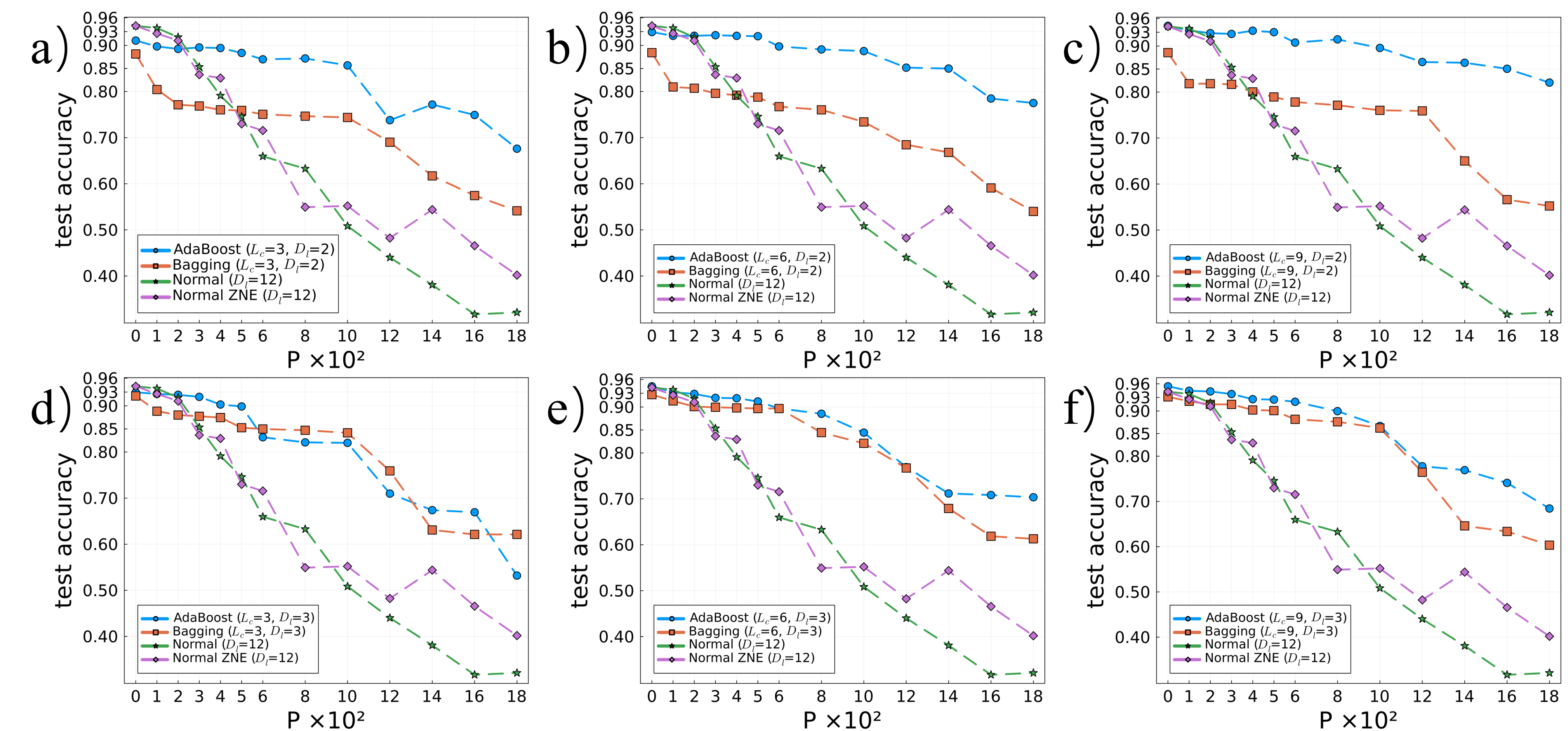
In this section, we consider noisy quantum computers in which controlled-not gates are noisy and operate according to Eq. (9). The strength of noise is quantified with decoherence rate , which affects all the two-qubit gates of the circuit equally. We compare four different scenarios: (i) a normal VQC with a deep circuit of layers without ZNE; (ii) a VQC with a deep circuit of layers with ZNE; (iii) Bagging VQC with shallow circuits of and layers with various numbers of classifiers; and (iv) AdaBoost VQC with shallow circuits of and layers with various numbers of classifiers. We first fix the circuit layer for Bagging and AdaBoost and plot the test accuracy as a function of decoherence rate in Figs. 5(a)-(c), for , and classifiers, respectively. As the figure shows, the test accuracy for a normal VQC with a deep circuit of decays rapidly as increases. ZNE can indeed enhance the accuracy for such a deep circuit, but for larger the decay is still significant. Interestingly, a shallow Bagging VQC with can outperform the deep circuit classifier even with ZNE when . Increasing the number of classifiers from to slightly improves the performance of Bagging. Remarkably, the AdaBoost algorithm with even shallow circuits of layers can outperform the other scenarios for noise rates of and remains stably high even for very strong decoherence rates up to .
Similarly, one can consider the Bagging and the AdaBoost with layers in Figs. 5(d)-(f) for , and classifiers, respectively. In this case, the Bagging and AdaBoost outperform deep circuits with ZNE when . As increases, the performance of Bagging and AdaBoost remains fairly close to each other for and classifiers. By increasing the number of classifiers or noise rate , again AdaBoost outperforms Bagging. Note that the AdaBoost algorithm is hugely benefited by increasing the number of classifiers due to its interconnected training method, which improves the classifiers based on the mistakes of the previous ones. Another interesting observation is that in very noisy quantum computers, i.e. large , AdaBoost with layers is better than AdaBoost with layers. This is because deeper circuits naturally have more two-qubit gates and thus are more susceptible to the effect of noise.
In summary, both our ensemble-learning error mitigation methods, namely Bagging VQC and AdaBoost VQC, provide a significant improvement over conventional ZNE method. This is a general behavior and can also be observed for rotation encoding of the input data (results not shown). Moreover, thanks to its interconnected training method, the AdaBoost algorithm can outperform the Bagging, in particular, when the number of classifiers increases. The AdaBoost accuracy enhancement over the other methods becomes even more pronounced when the quantum computer is subjected to strong decoherence, namely large .

III.4 Classification of Quantum Data
In this section, we apply our ensemble classification methods to a quantum dataset. The input data are quantum states which are taken from the ground state of a chain of qubits interacting via Hamiltonian
| (17) | |||||
| (18) |
where is the three-body spin coupling, is the two-body spin exchange interaction and is the magnetic field. Note that the three-body interaction term flips a central spin with the addition of a phase that depends on the quantum states of its neighbors. This Hamiltonian commutes with two string operators
| (19) |
This implies that the Hamiltonian has a symmetry which results in the emergence of a Symmetry-Protected Topological (SPT) phase which is described by a non-local order parameter Pollmann and Turner 2012; Haegeman et al. 2012. In Ref. Cong et al. 2019 the phase diagram of this Hamiltonian has been determined through density matrix renormalization group analysis McCulloch 2008. The Hamiltonian has three different phases as vary, namely antiferromagnetic, paramagnetic, and SPT phases. In the absence of two-body interaction, i.e. , the Hamiltonian becomes solvable via Jordan–Wigner transformation and shows a quantum phase transition from the SPT to the paramagnetic phase at a specific value of . Recently, the phase diagram of this system has also been determined through quantum convolution neural networks Cong et al. 2019 which has been experimentally realized in superconducting quantum computers for a system of size Beckey et al. 2022.
Here, we use our ensemble classification methods for determining the phase diagram of the system. The quantum circuit is exactly the same as before, shown in Fig. 1(a), with one important difference. Since the input is itself a quantum state, the encoder is no longer needed and the quantum state can directly be fed into the parameterized circuit. Similar to the approach of Ref. Cong et al. 2019, we only measure the last qubit despite having three phases, i.e. three classes. This method labels the phases as SPT and non-SPT phases. Since anti-ferromagnetic and paramagnetic phases are well separated and have no boundary they can be easily recognized in the phase diagram, as we will see in the following.
First, we focus on the Bagging algorithm for phase recognition of the SPT Hamiltonian with qubits using an ensemble of circuits with layers. We consider the phase diagram in the plane with the resolution of pixels. For training the circuit, We randomly select the ground states of random samples in the plane, as our training data. In Figs. 6(a)-(c) we plot the result of our Bagging VQC for an ensemble of , , and classifiers, respectively. The phase boundaries, computed by density matrix renormalization group McCulloch 2008; Cong et al. 2019, are plotted by the blue and red lines. As evident in the figures, Bagging VQC can indeed capture the phase diagram and the precision becomes better as the number of classifiers increases. It is worth emphasizing that for shallower circuits with the depth layers, the precision for capturing the phase diagram goes down (results not shown). In particular, the performance is poor for circuits with layers, no matter how many classifiers we use. This shows that increasing the number of classifiers alone cannot compensate the circuit dept. This is because the classifiers are trained independently and their weakness cannot be improved during training.
Second, we also exploit AdaBoost for capturing the phase diagram of the Hamiltonian with very shallow circuits of layers. Similar to the previous cases, we use the same circuit as shown in Fig. 1(a) without the encoder part. We use the same dataset that we used for the Bagging algorithm. In Figs. 6(d)-(f) we depict the phase diagram of the system using AdaBoost circuits with the depth of layers and , and classifiers, respectively. Note that the AdaBoost can only become effective for more than one classifier. As the figures clearly show, the AdaBoost protocol can indeed determine the phase diagram even with shallow circuits with only layers. As expected, the precision is improved as the number of classifiers increases. In particular, for the phase boundaries between the SPT and the other phases are captured quite precisely. The fact that circuits with only layers are enough for recognizing the phase boundaries already shows the superiority of AdaBoost VQC over Bagging VQC. As mentioned before, this is because in AdaBoost VQC the training of classifiers is not independent of each other in such a way that each classifier tries to correct the errors of the previous ones through weight updating.
IV CONCLUSIONS
We introduced two ensemble-learning error mitigation algorithms, namely Bagging and AdaBoost, for VQCs. These algorithms can significantly enhance the precision of classification using only shallow quantum circuits with very few parameters to train. Our protocols have been tested on both classical (handwriting digits) and quantum (the phase recognition of an SPT Hamiltonian) datasets. Considering imperfect NISQ computers, our ensemble-learning error mitigation methods significantly outperform the ZNE method in classification tasks. Thanks to its interconnecting training approach, which tends to correct the mistakes of one classifier in the training of the next one, the AdaBoost method achieves better accuracy and shows better robustness against noise than the Bagging algorithm. The superiority of AdaBoost over ZNE and Bagging becomes even more prominent when the number of classifiers increases, in particular at the large noise limit.
Our ensemble-learning error mitigation techniques are very general. For classification problems, they are applicable to both classical and quantum datasets and work for both amplitude and rotation encodings. The application of our ensemble-learning error mitigation methods is not limited to classification and can be generalized to other supervised machine-learning problems such as Kernel learning and regression. Moreover, it can also be used for non-variational classification methods such as quantum support vector machines. Our ensemble-learning VQCs are NISQ-friendly and very distinct from other ensemble-learning proposals Schuld and Petruccione 2018; Wang et al. 2020; Arunachalam and Maity 2020; Izdebski and de Wolf 2020; Macaluso et al. 2020 which are hardware demanding, relying on multi-qubit controlled unitaries and quantum subroutines such as quantum phase estimation, Grover search and quantum mean estimation.
Therefore, our approach can solve a broad category of machine learning problems with today’s NISQ technologies.
Acknowledgements.
The authors acknowledge support from the National Key R&D Program of China (Grant No. 2018YFA0306703). A.B. thanks the National Natural Science Foundation of China (Grants No. 12050410253, No. 92065115, and No. 12274059), and the Ministry of Science and Technology of China (Grant No. QNJ2021167001L) for their support. X.W. thanks the National Natural Science Foundation of China (Grant No. 92265208) for their support. Y.L. thanks the National Natural Science Foundation of China (Grant No. 12225507 and No. 12088101) for their support. We also thank Guanyu Zhou for helpful discussions and Chu Guo for package “VQC.jl”.*
APPENDIX A TRAINING THE QUANTUM CIRCUIT
For numerical simulations, we rely on Julia packages “VQC.jl” and “QuantumCircuit.jl”. In the training process of our VQCs, we use Adam optimizer Kingma and Ba 2017, which is a gradient-based method, with a learning rate of , to update the quantum circuit parameters . The gradients are obtained by Automatic differentiation methods supported by the VQC.jl package. The optimization iterations of the training procedure are times for the weak quantum classifiers in both AdaBoost VQC and Bagging VQC and times for the normal deep VQC. In order to be initialization-independent, for noise-free and noisy circuits, the performance is averaged over and random initial samples, respectively.
For quantum classification of the SPT Hamiltonian, the training dataset takes the ground state of random samples in the plane. To show the performance of the classifier, we depict the phase diagram with the resolution of averaged in the plane, as shown in Fig. 6. The optimization iteration is fixed to and each data point has been averaged over different random initial samples.
References
- Mitchell (1997) Tom M. Mitchell, Machine Learning (McGraw-Hill, New York, 1997).
- Kotsiantis (2007) S. B. Kotsiantis, “Supervised machine learning: A review of classification techniques,” in Proceedings of the 2007 Conference on Emerging Artificial Intelligence Applications in Computer Engineering: Real Word AI Systems with Applications in EHealth, HCI, Information Retrieval and Pervasive Technologies (IOS Press, NLD, 2007) p. 3–24.
- Zhang and Zhou (2014) Min-Ling Zhang and Zhi-Hua Zhou, “A review on multi-label learning algorithms,” IEEE Trans Knowl Data Eng 26, 1819–1837 (2014).
- Tolles and Meurer (2016) Juliana Tolles and William J. Meurer, “Logistic Regression: Relating Patient Characteristics to Outcomes,” JAMA 316, 533 (2016).
- Quinlan (1986) J. R. Quinlan, “Induction of decision trees,” Mach Learn 1, 81–106 (1986).
- Cover and Hart (1967) T. Cover and P. Hart, “Nearest neighbor pattern classification,” IEEE Trans. Inf. Theory 13, 21–27 (1967).
- Cortes and Vapnik (1995) Corinna Cortes and Vladimir Vapnik, “Support-vector networks,” Mach Learn 20, 273–297 (1995).
- Zhang (2000) G.P. Zhang, “Neural networks for classification: a survey,” IEEE Trans. Syst. Man Cybern. Syst. 30, 451–462 (2000).
- Breiman (1996) Leo Breiman, “Bagging predictors,” Machine Learning 24, 123–140 (1996).
- Freund and Schapire (1995) Yoav Freund and Robert E. Schapire, “A desicion-theoretic generalization of on-line learning and an application to boosting,” in Computational Learning Theory, edited by Paul Vitányi (Springer Berlin Heidelberg, Berlin, Heidelberg, 1995) pp. 23–37.
- Hastie et al. (2009) Trevor Hastie, Saharon Rosset, Ji Zhu, and Hui Zou, “Multi-class AdaBoost,” Stat Interface 2, 349–360 (2009).
- Barends et al. (2016) R. Barends, A. Shabani, L. Lamata, J. Kelly, A. Mezzacapo, U. Las Heras, R. Babbush, A. G. Fowler, B. Campbell, Yu Chen, Z. Chen, B. Chiaro, A. Dunsworth, E. Jeffrey, E. Lucero, A. Megrant, J. Y. Mutus, M. Neeley, C. Neill, P. J. J. O’Malley, C. Quintana, P. Roushan, D. Sank, A. Vainsencher, J. Wenner, T. C. White, E. Solano, H. Neven, and John M. Martinis, “Digitized adiabatic quantum computing with a superconducting circuit,” Nature 534, 222–226 (2016).
- Hensgens et al. (2017) T. Hensgens, T. Fujita, L. Janssen, Xiao Li, C. J. Van Diepen, C. Reichl, W. Wegscheider, S. Das Sarma, and L. M. K. Vandersypen, “Quantum simulation of a Fermi–Hubbard model using a semiconductor quantum dot array,” Nature 548, 70–73 (2017).
- Arute et al. (2019) Frank Arute, Kunal Arya, Ryan Babbush, Dave Bacon, Joseph C Bardin, Rami Barends, Rupak Biswas, Sergio Boixo, Fernando GSL Brandao, David A Buell, et al., “Quantum supremacy using a programmable superconducting processor,” Nature 574, 505–510 (2019).
- Arute et al. (2020) Frank Arute, Kunal Arya, Ryan Babbush, Dave Bacon, Joseph C Bardin, Rami Barends, Rupak Biswas, Sergio Boixo, Fernando GSL Brandao, David A Buell, et al., “Hartree-fock on a superconducting qubit quantum computer,” Science 369, 1084–1089 (2020).
- Wu et al. (2021) Yulin Wu, Wan-Su Bao, Sirui Cao, Fusheng Chen, Ming-Cheng Chen, Xiawei Chen, Tung-Hsun Chung, Hui Deng, Yajie Du, Daojin Fan, et al., “Strong quantum computational advantage using a superconducting quantum processor,” Phys. Rev. Lett. 127, 180501 (2021).
- Bravyi et al. (2022) Sergey Bravyi, Oliver Dial, Jay M Gambetta, Dario Gil, and Zaira Nazario, “The future of quantum computing with superconducting qubits,” J. Appl. Phys. 132, 160902 (2022).
- Hempel et al. (2018) Cornelius Hempel, Christine Maier, Jonathan Romero, Jarrod McClean, Thomas Monz, Heng Shen, Petar Jurcevic, Ben P. Lanyon, Peter Love, Ryan Babbush, Alán Aspuru-Guzik, Rainer Blatt, and Christian F. Roos, “Quantum Chemistry Calculations on a Trapped-Ion Quantum Simulator,” Phys. Rev. X 8, 031022 (2018).
- Kokail et al. (2019) Christian Kokail, Christine Maier, Rick van Bijnen, Tiff Brydges, Manoj K Joshi, Petar Jurcevic, Christine A Muschik, Pietro Silvi, Rainer Blatt, Christian F Roos, et al., “Self-verifying variational quantum simulation of lattice models,” Nature 569, 355–360 (2019).
- Ringbauer et al. (2022) Martin Ringbauer, Michael Meth, Lukas Postler, Roman Stricker, Rainer Blatt, Philipp Schindler, and Thomas Monz, “A universal qudit quantum processor with trapped ions,” Nat. Phys. 18, 1053–1057 (2022).
- Noel et al. (2022) Crystal Noel, Pradeep Niroula, Daiwei Zhu, Andrew Risinger, Laird Egan, Debopriyo Biswas, Marko Cetina, Alexey V Gorshkov, Michael J Gullans, David A Huse, et al., “Measurement-induced quantum phases realized in a trapped-ion quantum computer,” Nat. Phys. 18, 760–764 (2022).
- Monroe et al. (2021) C. Monroe, W. C. Campbell, L.-M. Duan, Z.-X. Gong, A. V. Gorshkov, P. W. Hess, R. Islam, K. Kim, N. M. Linke, G. Pagano, P. Richerme, C. Senko, and N. Y. Yao, “Programmable quantum simulations of spin systems with trapped ions,” Rev. Mod. Phys. 93, 025001 (2021).
- Schreiber et al. (2015) Michael Schreiber, Sean S. Hodgman, Pranjal Bordia, Henrik P. Lüschen, Mark H. Fischer, Ronen Vosk, Ehud Altman, Ulrich Schneider, and Immanuel Bloch, “Observation of many-body localization of interacting fermions in a quasirandom optical lattice,” Science 349, 842–845 (2015).
- Gross and Bloch (2017) Christian Gross and Immanuel Bloch, “Quantum simulations with ultracold atoms in optical lattices,” Science 357, 995–1001 (2017).
- Sompet et al. (2022) Pimonpan Sompet, Sarah Hirthe, Dominik Bourgund, Thomas Chalopin, Julian Bibo, Joannis Koepsell, Petar Bojović, Ruben Verresen, Frank Pollmann, Guillaume Salomon, et al., “Realizing the symmetry-protected haldane phase in fermi–hubbard ladders,” Nature 606, 484–488 (2022).
- Saffman (2016) M Saffman, “Quantum computing with atomic qubits and Rydberg interactions: progress and challenges,” J PHYS B-AT MOL OPT 49, 202001 (2016).
- Aspuru-Guzik and Walther (2012) Alán Aspuru-Guzik and Philip Walther, “Photonic quantum simulators,” Nat. Phys 8, 285–291 (2012).
- Zhong et al. (2020) Han-Sen Zhong, Hui Wang, Yu-Hao Deng, Ming-Cheng Chen, Li-Chao Peng, Yi-Han Luo, Jian Qin, Dian Wu, Xing Ding, Yi Hu, Peng Hu, Xiao-Yan Yang, Wei-Jun Zhang, Hao Li, Yuxuan Li, Xiao Jiang, Lin Gan, Guangwen Yang, Lixing You, Zhen Wang, Li Li, Nai-Le Liu, Chao-Yang Lu, and Jian-Wei Pan, “Quantum computational advantage using photons,” Science 370, 1460–1463 (2020).
- Dai et al. (2022) Tianxiang Dai, Yutian Ao, Jueming Bao, Jun Mao, Yulin Chi, Zhaorong Fu, Yilong You, Xiaojiong Chen, Chonghao Zhai, Bo Tang, et al., “Topologically protected quantum entanglement emitters,” Nat. Photonics 16, 248–257 (2022).
- Daley et al. (2022) Andrew J Daley, Immanuel Bloch, Christian Kokail, Stuart Flannigan, Natalie Pearson, Matthias Troyer, and Peter Zoller, “Practical quantum advantage in quantum simulation,” Nature 607, 667–676 (2022).
- Schuld et al. (2017) M. Schuld, M. Fingerhuth, and F. Petruccione, “Implementing a distance-based classifier with a quantum interference circuit,” EPL 119, 60002 (2017).
- Rebentrost et al. (2014) Patrick Rebentrost, Masoud Mohseni, and Seth Lloyd, “Quantum Support Vector Machine for Big Data Classification,” Phys. Rev. Lett. 113, 130503 (2014).
- Li et al. (2015) Zhaokai Li, Xiaomei Liu, Nanyang Xu, and Jiangfeng Du, “Experimental realization of a quantum support vector machine,” Phys. Rev. Lett. 114, 140504 (2015).
- Lloyd et al. (2013) Seth Lloyd, Masoud Mohseni, and Patrick Rebentrost, “Quantum algorithms for supervised and unsupervised machine learning,” arXiv preprint arXiv:1307.0411 (2013).
- Wiebe et al. (2015) Nathan Wiebe, Ashish Kapoor, and Krysta M. Svore, “Quantum algorithms for nearest-neighbor methods for supervised and unsupervised learning,” Quantum Info. Comput. 15, 316–356 (2015).
- Lu and Braunstein (2014) Songfeng Lu and Samuel L. Braunstein, “Quantum decision tree classifier,” Quantum Inf Process 13, 757–770 (2014).
- Farhi and Gutmann (1998) Edward Farhi and Sam Gutmann, “Quantum computation and decision trees,” Phys. Rev. A 58, 915–928 (1998).
- Grant et al. (2018) Edward Grant, Marcello Benedetti, Shuxiang Cao, Andrew Hallam, Joshua Lockhart, Vid Stojevic, Andrew G. Green, and Simone Severini, “Hierarchical quantum classifiers,” NPJ Quantum Inf. 4, 65 (2018).
- Schuld et al. (2020a) Maria Schuld, Alex Bocharov, Krysta M. Svore, and Nathan Wiebe, “Circuit-centric quantum classifiers,” Phys. Rev. A 101, 032308 (2020a).
- Farhi and Neven (2018) Edward Farhi and Hartmut Neven, “Classification with quantum neural networks on near term processors,” arXiv preprint arXiv:1802.06002 (2018).
- Cong et al. (2019) Iris Cong, Soonwon Choi, and Mikhail D. Lukin, “Quantum convolutional neural networks,” Nat. Phys. 15, 1273–1278 (2019).
- Killoran et al. (2019) Nathan Killoran, Thomas R. Bromley, Juan Miguel Arrazola, Maria Schuld, Nicolás Quesada, and Seth Lloyd, “Continuous-variable quantum neural networks,” Phys. Rev. Res. 1, 033063 (2019).
- Romero et al. (2017) Jonathan Romero, Jonathan P Olson, and Alan Aspuru-Guzik, “Quantum autoencoders for efficient compression of quantum data,” Quantum Sci. Technol. 2, 045001 (2017).
- Zoufal et al. (2019) Christa Zoufal, Aurélien Lucchi, and Stefan Woerner, “Quantum generative adversarial networks for learning and loading random distributions,” NPJ Quantum Inf. 5, 1–9 (2019).
- Hou et al. (2022) Xiaokai Hou, Guanyu Zhou, Qingyu Li, Shan Jin, and Xiaoting Wang, “A duplication-free quantum neural network for universal approximation,” arXiv preprint arXiv:2211.11228 (2022).
- Liu et al. (2021) Junhua Liu, Kwan Hui Lim, Kristin L Wood, Wei Huang, Chu Guo, and He-Liang Huang, “Hybrid quantum-classical convolutional neural networks,” SCI CHINA PHYS MECH 64, 1–8 (2021).
- Bharti et al. (2022a) Kishor Bharti, Alba Cervera-Lierta, Thi Ha Kyaw, Tobias Haug, Sumner Alperin-Lea, Abhinav Anand, Matthias Degroote, Hermanni Heimonen, Jakob S. Kottmann, Tim Menke, Wai-Keong Mok, Sukin Sim, Leong-Chuan Kwek, and Alán Aspuru-Guzik, “Noisy intermediate-scale quantum algorithms,” Rev. Mod. Phys. 94, 015004 (2022a).
- Bharti et al. (2022b) Kishor Bharti, Alba Cervera-Lierta, Thi Ha Kyaw, Tobias Haug, Sumner Alperin-Lea, Abhinav Anand, Matthias Degroote, Hermanni Heimonen, Jakob S. Kottmann, Tim Menke, Wai-Keong Mok, Sukin Sim, Leong-Chuan Kwek, and Alán Aspuru-Guzik, “Noisy intermediate-scale quantum algorithms,” Rev. Mod. Phys. 94, 015004 (2022b).
- Cerezo et al. (2021) M. Cerezo, Andrew Arrasmith, Ryan Babbush, Simon C. Benjamin, Suguru Endo, Keisuke Fujii, Jarrod R. McClean, Kosuke Mitarai, Xiao Yuan, Lukasz Cincio, and Patrick J. Coles, “Variational quantum algorithms,” Nat. Rev. Phys. 3, 625–644 (2021).
- Peruzzo et al. (2014) Alberto Peruzzo, Jarrod McClean, Peter Shadbolt, Man-Hong Yung, Xiao-Qi Zhou, Peter J. Love, Alán Aspuru-Guzik, and Jeremy L. O’Brien, “A variational eigenvalue solver on a photonic quantum processor,” Nat. Commun. 5, 4213 (2014).
- Kandala et al. (2017) Abhinav Kandala, Antonio Mezzacapo, Kristan Temme, Maika Takita, Markus Brink, Jerry M. Chow, and Jay M. Gambetta, “Hardware-efficient variational quantum eigensolver for small molecules and quantum magnets,” Nature 549, 242–246 (2017).
- Higgott et al. (2019) Oscar Higgott, Daochen Wang, and Stephen Brierley, “Variational Quantum Computation of Excited States,” Quantum 3, 156 (2019).
- Wang et al. (2019) Daochen Wang, Oscar Higgott, and Stephen Brierley, “Accelerated variational quantum eigensolver,” Phys. Rev. Lett. 122, 140504 (2019).
- Lyu et al. (2020) Chufan Lyu, Victor Montenegro, and Abolfazl Bayat, “Accelerated variational algorithms for digital quantum simulation of many-body ground states,” Quantum 4, 324 (2020).
- Lyu et al. (2023) Chufan Lyu, Xusheng Xu, Man-Hong Yung, and Abolfazl Bayat, “Symmetry enhanced variational quantum spin eigensolver,” Quantum 7, 899 (2023).
- Biamonte et al. (2017) Jacob Biamonte, Peter Wittek, Nicola Pancotti, Patrick Rebentrost, Nathan Wiebe, and Seth Lloyd, “Quantum machine learning,” Nature 549, 195–202 (2017).
- Mitarai et al. (2018) K. Mitarai, M. Negoro, M. Kitagawa, and K. Fujii, “Quantum circuit learning,” Phys. Rev. A 98, 032309 (2018).
- Lu et al. (2020) Sirui Lu, Lu-Ming Duan, and Dong-Ling Deng, “Quantum adversarial machine learning,” Phys. Rev. Res. 2, 033212 (2020).
- Du et al. (2021) Yuxuan Du, Min-Hsiu Hsieh, Tongliang Liu, Dacheng Tao, and Nana Liu, “Quantum noise protects quantum classifiers against adversaries,” Phys. Rev. Res. 3, 023153 (2021).
- Liu and Wittek (2020) Nana Liu and Peter Wittek, “Vulnerability of quantum classification to adversarial perturbations,” Phys. Rev. A 101, 062331 (2020).
- Ren et al. (2022) Wenhui Ren, Weikang Li, Shibo Xu, Ke Wang, Wenjie Jiang, Feitong Jin, Xuhao Zhu, Jiachen Chen, Zixuan Song, Pengfei Zhang, et al., “Experimental quantum adversarial learning with programmable superconducting qubits,” Nat. Comput. Sci. 2, 711–717 (2022).
- Farhi et al. (2014) Edward Farhi, Jeffrey Goldstone, and Sam Gutmann, “A quantum approximate optimization algorithm,” arXiv preprint arXiv:1411.4028 (2014).
- Bravo-Prieto et al. (2020) Carlos Bravo-Prieto, Ryan LaRose, M. Cerezo, Yigit Subasi, Lukasz Cincio, and Patrick J. Coles, “Variational quantum linear solver,” arXiv preprint arXiv:1909.05820 (2020).
- Xu et al. (2021) Xiaosi Xu, Jinzhao Sun, Suguru Endo, Ying Li, Simon C. Benjamin, and Xiao Yuan, “Variational algorithms for linear algebra,” Sci. Bull. 66, 2181–2188 (2021).
- Huang et al. (2021) Hsin-Yuan Huang, Kishor Bharti, and Patrick Rebentrost, “Near-term quantum algorithms for linear systems of equations with regression loss functions,” New J. Phys. 23, 113021 (2021).
- Beckey et al. (2022) Jacob L. Beckey, M. Cerezo, Akira Sone, and Patrick J. Coles, “Variational quantum algorithm for estimating the quantum Fisher information,” Phys. Rev. Research 4, 013083 (2022).
- Kaubruegger et al. (2019) Raphael Kaubruegger, Pietro Silvi, Christian Kokail, Rick van Bijnen, Ana Maria Rey, Jun Ye, Adam M. Kaufman, and Peter Zoller, “Variational Spin-Squeezing Algorithms on Programmable Quantum Sensors,” Phys. Rev. Lett. 123, 260505 (2019).
- Meyer et al. (2021) Johannes Jakob Meyer, Johannes Borregaard, and Jens Eisert, “A variational toolbox for quantum multi-parameter estimation,” NPJ Quantum Inf. 7, 89 (2021).
- Banchi (2022) Leonardo Banchi, “Robust quantum classifiers via NISQ adversarial learning,” Nat Comput Sci 2, 699–700 (2022).
- Schuld et al. (2020b) Maria Schuld, Alex Bocharov, Krysta M. Svore, and Nathan Wiebe, “Circuit-centric quantum classifiers,” Phys. Rev. A 101, 032308 (2020b).
- Deng (2021) Dong-Ling Deng, “Quantum enhanced convolutional neural networks for NISQ computers,” SCI CHINA PHYS MECH 64, 100331 (2021).
- Gong and Deng (2021) Weiyuan Gong and Dong-Ling Deng, “Universal adversarial examples and perturbations for quantum classifiers,” Natl. Sci. Rev. , nwab130 (2021).
- Uvarov et al. (2020) A. V. Uvarov, A. S. Kardashin, and J. D. Biamonte, “Machine learning phase transitions with a quantum processor,” Phys. Rev. A 102, 012415 (2020).
- Herrmann et al. (2022) Johannes Herrmann, Sergi Masot Llima, Ants Remm, Petr Zapletal, Nathan A. McMahon, Colin Scarato, François Swiadek, Christian Kraglund Andersen, Christoph Hellings, Sebastian Krinner, et al., “Realizing quantum convolutional neural networks on a superconducting quantum processor to recognize quantum phases,” Nat. Commun. 13, 4144 (2022).
- Havlíček et al. (2019) Vojtěch Havlíček, Antonio D. Córcoles, Kristan Temme, Aram W. Harrow, Abhinav Kandala, Jerry M. Chow, and Jay M. Gambetta, “Supervised learning with quantum-enhanced feature spaces,” Nature 567, 209–212 (2019).
- Li and Benjamin (2017) Ying Li and Simon C. Benjamin, “Efficient variational quantum simulator incorporating active error minimization,” Phys. Rev. X 7, 021050 (2017).
- Temme et al. (2017) Kristan Temme, Sergey Bravyi, and Jay M. Gambetta, “Error Mitigation for Short-Depth Quantum Circuits,” Phys. Rev. Lett. 119, 180509 (2017).
- Kandala et al. (2019) Abhinav Kandala, Kristan Temme, Antonio D. Córcoles, Antonio Mezzacapo, Jerry M. Chow, and Jay M. Gambetta, “Error mitigation extends the computational reach of a noisy quantum processor,” Nature 567, 491–495 (2019).
- Endo et al. (2021) Suguru Endo, Zhenyu Cai, Simon C. Benjamin, and Xiao Yuan, “Hybrid Quantum-Classical Algorithms and Quantum Error Mitigation,” J. Phys. Soc. Jpn. 90, 032001 (2021).
- Qin et al. (2022a) Dayue Qin, Xiaosi Xu, and Ying Li, “An overview of quantum error mitigation formulas,” Chin. Phys. B 31, 090306 (2022a).
- Cai et al. (2022) Zhenyu Cai, Ryan Babbush, Simon C Benjamin, Suguru Endo, William J Huggins, Ying Li, Jarrod R McClean, and Thomas E O’Brien, “Quantum error mitigation,” arXiv preprint arXiv:2210.00921 (2022).
- Schuld and Petruccione (2018) Maria Schuld and Francesco Petruccione, “Quantum ensembles of quantum classifiers,” Sci Rep 8, 2772 (2018).
- Wang et al. (2020) XiMing Wang, YueChi Ma, Min-Hsiu Hsieh, and Man-Hong Yung, “Quantum speedup in adaptive boosting of binary classification,” Sci. China Phys. Mech. Astron. 64, 220311 (2020).
- Arunachalam and Maity (2020) Srinivasan Arunachalam and Reevu Maity, “Quantum Boosting,” in Proceedings of the 37th International Conference on Machine Learning (PMLR, 2020) pp. 377–387.
- Izdebski and de Wolf (2020) Adam Izdebski and Ronald de Wolf, “Improved Quantum Boosting,” (2020), 10.48550/arXiv.2009.08360, arXiv:2009.08360 [quant-ph] version: 1.
- Macaluso et al. (2020) Antonio Macaluso, Luca Clissa, Stefano Lodi, and Claudio Sartori, “Quantum ensemble for classification,” arXiv preprint arXiv:2007.01028 (2020).
- Kitaev (1995) A. Yu Kitaev, “Quantum measurements and the Abelian Stabilizer Problem,” arXiv preprint quant-ph/9511026 (1995).
- Nayak and Wu (1999) Ashwin Nayak and Felix Wu, “The quantum query complexity of approximating the median and related statistics,” in Proceedings of the Thirty-First Annual ACM Symposium on Theory of Computing, STOC ’99 (Association for Computing Machinery, New York, NY, USA, 1999) p. 384–393.
- Brassard et al. (2011) Gilles Brassard, Frederic Dupuis, Sebastien Gambs, and Alain Tapp, “An optimal quantum algorithm to approximate the mean and its application for approximating the median of a set of points over an arbitrary distance,” arXiv preprint arXiv:1106.4267 (2011).
- Grover (1996) Lov K. Grover, “A fast quantum mechanical algorithm for database search,” in Proceedings of the Twenty-Eighth Annual ACM Symposium on Theory of Computing, STOC ’96 (Association for Computing Machinery, New York, NY, USA, 1996) p. 212–219.
- Qin et al. (2022b) Ruiyang Qin, Zhiding Liang, Jinglei Cheng, Peter Kogge, and Yiyu Shi, “Improving quantum classifier performance in nisq computers by voting strategy from ensemble learning,” arXiv preprint arXiv:2210.01656 (2022b).
- Casares (2020) Pablo Antonio Moreno Casares, “Circuit implementation of bucket brigade qram for quantum state preparation,” arXiv preprint arXiv:2006.11761 (2020).
- Jiang et al. (2019) N. Jiang, Y.-F. Pu, W. Chang, C. Li, S. Zhang, and L.-M. Duan, “Experimental realization of 105-qubit random access quantum memory,” NPJ Quantum Inf. 5, 28 (2019).
- Park et al. (2019) Daniel K. Park, Francesco Petruccione, and June-Koo Kevin Rhee, “Circuit-Based Quantum Random Access Memory for Classical Data,” Sci Rep 9, 3949 (2019).
- Giovannetti et al. (2008) Vittorio Giovannetti, Seth Lloyd, and Lorenzo Maccone, “Quantum Random Access Memory,” Phys. Rev. Lett. 100, 160501 (2008).
- Schuld et al. (2021) Maria Schuld, Ryan Sweke, and Johannes Jakob Meyer, “Effect of data encoding on the expressive power of variational quantum-machine-learning models,” Phys. Rev. A 103, 032430 (2021).
- LaRose and Coyle (2020) Ryan LaRose and Brian Coyle, “Robust data encodings for quantum classifiers,” Phys. Rev. A 102, 032420 (2020).
- Kingma and Ba (2017) Diederik P. Kingma and Jimmy Ba, “Adam: A method for stochastic optimization,” arXiv preprint arXiv:1412.6980 (2017).
- Dua and Graff (2017) Dheeru Dua and Casey Graff, “UCI machine learning repository,” (2017).
- Bao et al. (2022) Feng Bao, Hao Deng, Dawei Ding, Ran Gao, Xun Gao, Cupjin Huang, Xun Jiang, Hsiang-Sheng Ku, Zhisheng Li, Xizheng Ma, et al., “Fluxonium: An alternative qubit platform for high-fidelity operations,” Phys. Rev. Lett. 129, 010502 (2022).
- Giurgica-Tiron et al. (2020) Tudor Giurgica-Tiron, Yousef Hindy, Ryan LaRose, Andrea Mari, and William J Zeng, “Digital zero noise extrapolation for quantum error mitigation,” in 2020 IEEE International Conference on Quantum Computing and Engineering (QCE) (IEEE, 2020) pp. 306–316.
- Sagi and Rokach (2018) Omer Sagi and Lior Rokach, “Ensemble learning: A survey,” Wiley Interdiscip Rev Data Min Knowl Discov 8, e1249 (2018).
- McCulloch (2008) Ian P McCulloch, “Infinite size density matrix renormalization group, revisited,” arXiv preprint arXiv:0804.2509 (2008).
- Pollmann and Turner (2012) Frank Pollmann and Ari M. Turner, “Detection of symmetry-protected topological phases in one dimension,” Phys. Rev. B 86, 125441 (2012).
- Haegeman et al. (2012) Jutho Haegeman, David Pérez-García, Ignacio Cirac, and Norbert Schuch, “Order parameter for symmetry-protected phases in one dimension,” Phys. Rev. Lett. 109, 050402 (2012).