SeeGera: Self-supervised Semi-implicit Graph Variational Auto-encoders with MaskingConference: Proceedings of the ACM Web Conference 2023; May 1–5, 2023; Austin, TX, USAProceedings of the ACM Web Conference 2023 (WWW ’23), May 1–5, 2023, Austin, TX, USAPrice: 15.00DOI: 10.1145/3543507.3583245ISBN: 978-1-4503-9416-1/23/04
Abstract.
Generative graph self-supervised learning (SSL) aims to learn node representations by reconstructing the input graph data. However, most existing methods focus on unsupervised learning tasks only and very few work has shown its superiority over the state-of-the-art graph contrastive learning (GCL) models, especially on the classification task. While a very recent model has been proposed to bridge the gap, its performance on unsupervised learning tasks is still unknown. In this paper, to comprehensively enhance the performance of generative graph SSL against other GCL models on both unsupervised and supervised learning tasks, we propose the SeeGera model, which is based on the family of self-supervised variational graph auto-encoder (VGAE). Specifically, SeeGera adopts the semi-implicit variational inference framework, a hierarchical variational framework, and mainly focuses on feature reconstruction and structure/feature masking. On the one hand, SeeGera co-embeds both nodes and features in the encoder and reconstructs both links and features in the decoder. Since feature embeddings contain rich semantic information on features, they can be combined with node embeddings to provide fine-grained knowledge for feature reconstruction. On the other hand, SeeGera adds an additional layer for structure/feature masking to the hierarchical variational framework, which boosts the model generalizability. We conduct extensive experiments comparing SeeGera with 9 other state-of-the-art competitors. Our results show that SeeGera can compare favorably against other state-of-the-art GCL methods in a variety of unsupervised and supervised learning tasks.
Keywords:
Graph neural networks, graph self-supervised learning, variational graph auto-encoder1. Introduction
Self-supervised learning (SSL) (He et al. 2020; Devlin et al. 2018; You et al. 2020b; Hu et al. 2020) has attracted significant attention recently. By extracting and employing supervisions from data itself, SSL can heavily reduce the dependence of neural network models on the labeled data, which is costly to obtain. To facilitate graph-based learning, SSL has been applied on graph-structured data. For example, it can learn representations for nodes (e.g., web pages in search engines), and detect the anomalies on webs (e.g., malicious users) (Liu et al. 2021). Recently, graph contrastive learning (GCL), as one of the main SSL types, has experienced a surge (Velickovic et al. 2019; Sun et al. 2019; You et al. 2020a; Jiao et al. 2020). The core idea of GCL is to first construct positive and negative pairs for nodes, and then maximize the similarity between positive pairs while minimizing that between negative ones11 1 Note that some GCL methods require positive pairs only and they only maximize the similarity between positive pairs..
Despite the success, existing GCL methods suffer from two main problems. On the one hand, negative samples are needed in most contrastive objectives, which generally construct one positive and negative samples for each node. However, these models are easily affected by the value of . When is small, the model cannot learn sufficient discriminative information, which degrades the model effectiveness; otherwise, there could lead to a large number of false-negative samples and slow convergence. Generally, is set empirically and there lack theoretical supports. On the other hand, for the rest of methods based on positive pairs only, they are easily trapped into a degenerate solution (Zhu et al. 2021a), where all the output embeddings of nodes collapse to a constant. To tackle the issue, additional strategies are necessary, such as asymmetric dual encoders with momentum updates and exponential moving average (Qiu et al. 2020; Thakoor et al. 2021). Recently, some studies (Li et al. 2022) have showed that although these training strategies can alleviate collapse to some extent, they may still cause collapse in partial dimensions of the representation, which leads to worse performance.
To address the shortcomings of GCL methods, generative graph SSL methods can be used instead. In particular, self-supervised graph auto-encoders (GAEs) (Kipf and Welling 2016), whose objective is to reconstruct the input graph data, have been widely studied. Existing methods mainly differ in their adopted reconstruction components, such as the adjacency matrix reconstruction (Pan et al. 2018), the node feature reconstruction (Park et al. 2019) and a combination of both graph structure and node feature reconstruction (Salehi and Davulcu 2019). However, most of these methods focus on the unsupervised learning tasks like link prediction and node clustering, and very few work has shown its superiority over the state-of-the-art GCL methods, especially on the classification task. While a masked GAE model GraphMAE (Hou et al. 2022) is very recently proposed to bridge the gap, its performance on the unsupervised learning tasks is still unexplored. Since the goal of SSL is to learn versatile representations, a further study on self-supervised GAE model that can achieve comprehensive superiority on both unsupervised and supervised learning tasks is needed. Further, although GraphMAE is an auto-encoding method, it is based on GAE and is essentially not a generative model. This also calls our attention back to the study of generative graph SSL model, such as variational graph auto-encoder (VGAE) (Kipf and Welling 2016).
Different from GAE, VGAE consists of an inference model and a generative model. Specifically, the inference model encodes observations (links and features) into latent variables (node embeddings) while the generative model decodes from these latent variables to reconstruct links. However, as pointed out in (Hou et al. 2022), node feature reconstruction is beneficial for learning high-quality representations. Therefore, the lack of feature reconstruction could degrade the model effectiveness. To solve the issue, most existing methods adopt MLP (Hu et al. 2019; Hu et al. 2020) and GNNs (Hou et al. 2022; Park et al. 2019) as their decoders for feature reconstruction. However, they utilize node-level embeddings only and ignore feature-level embeddings that contain rich semantic information on node features and can be used to help feature reconstruction. Recently, CAN (Meng et al. 2019) is proposed to co-embed both nodes and features, and use the inner product of their embeddings as the decoder to recover node features. Despite the success, it has three main problems. First, the linear decoder is generally less powerful than MLP and GNNs, which restricts the model’s capability in reconstructing node features. Second, it assumes the independence between node and feature embeddings in the variational inference stage, but practically these two types of embeddings are highly correlated. Third, it lacks structure/feature masking in the learning process, which has been shown to degrade the model’s performance on the classification task (Hou et al. 2022).
In this paper, we study generative graph SSL and our goal is to enhance the family of self-supervised VGAE on graph representation learning in a variety of downstream tasks. Recently, semi-implicit variational inference (SIVI) (Yin and Zhou 2018), which is a hierarchical variational framework, has been applied to VGAE to model a wide range of underlying true posteriors with multi-modality, skewness and heavy tails (Hasanzadeh et al. 2019). We thus adopt the framework to remove the explicit Gaussian restriction on the variational distribution and mainly focus on the component of feature reconstruction and structure/feature masking. We propose a Self-supervised semi-implicit Graph variational auto-encoder with masking, namely, SeeGera. Specifically, the model co-embeds both nodes and features in the encoder and jointly reconstructs links and features in the decoder. Note that the feature embeddings can provide fine-grained information that is supplementary to the node embeddings when reconstructing node features. Specifically, for each node, we take its feature values as weights and compute the weighted average of feature embeddings w.r.t. the node. The weighted embedding characterizes the affinities between the node and all the features. After that, we combine the weighted embedding with the node embedding, and feed the fused embedding into GNNs to reconstruct the node’s features. Further, to generate node and feature embeddings in the encoder, we first assume the independence between them and propose the base SeeGera model. Then we upgrade the model by capturing the correlations between node and feature embeddings. Finally, we add an additional layer to the hierarchical variational framework to integrate SeeGera with the masking mechanism and boost the model performance. In summary, our main contributions are listed:
We propose a generative graph SSL model SeeGera. To our knowledge, this is the first generative graph SSL method that is comprehensively compared with the SOTA GCL models in terms of both unsupervised and supervised learning tasks, and shows superiority.
We present a novel feature reconstruction method that leverages both node and feature embeddings to provide fine-grained information for reconstructing features. We further introduce the structure/feature masking mechanism by adding an additional layer to the hierarchical variational framework.
We conduct extensive experiments to evaluate the performance of SeeGera on two unsupervised learning tasks: link prediction and attribute inference, and one supervised learning task: node classification. Experimental results show that SeeGera can significantly outperform other competitors on both link prediction and attribute inference tasks, and perform comparably with them in node classification. This effectively verifies the power of generative graph SSL in graph representation learning.
2. Related Work
In this section, we summarize the related work on both graph self-supervised learning and generative graph self-supervised learning, respectively.
2.1. Graph self-supervised learning
Graph self-supervised learning (Sun et al. 2019; You et al. 2020a; Hou et al. 2022; Xu et al. 2021) aims to employ supervisions extracted from graph-structured data without the need for annotated data. Existing methods can be mainly divided into four types: (1) generative models (Kipf and Welling 2016), whose objective is to reconstruct the input graph data. (2) auxiliary-property-based methods (You et al. 2020b), which first obtain graph-related properties and then take them as supervisions, such as the pseudo labels of unlabeled nodes; (3) contrastive models (Velickovic et al. 2019), which construct positive and negative pairs for contrast. (4) hybrid approaches (Zhang et al. 2020), which combine the objectives of the first three types in a multi-task learning fashion. For a comprehensive survey on graph self-supervised learning, see (Liu et al. 2022).
Recently, graph contrastive learning has been widely studied. According to whether negative samples are used in the learning process, existing methods include negative-sample-based and negative-sample-free ones. For the former, DGI (Velickovic et al. 2019) and InfoGraph (Sun et al. 2019) employ corruptions to construct negative pairs. GRACE (Zhu et al. 2020), GCA (Zhu et al. 2021b) and GraphCL (You et al. 2020a) take samples in a mini-batch as a dictionary whose size is constrained by the batch size and consider other samples in the same mini-batch as negatives of a sample, while GCC (Qiu et al. 2020) maintains a dynamic dictionary with larger size as in MoCo (He et al. 2020). For the latter, BGRL (Thakoor et al. 2021) and CCA-SSG (Zhang et al. 2021) are two representative models that are based on asymmetric encoding architectures. However, they require special training strategies to avoid the collapse of learned node embeddings to a constant, such as momentum update (He et al. 2020), exponential moving average (Thakoor et al. 2021) and stop gradient (Thakoor et al. 2021). Further, existing GCL methods heavily rely on graph augmentation strategies to construct different graph views for contrast, including feature-oriented (e.g., masking (You et al. 2020a) and shuffling (Velickovic et al. 2019)), proximity-oriented (e.g., perturbation (You et al. 2020a)), and graph-sampling-based (e.g., random-walk (Hassani and Khasahmadi 2020)) augmentations.
2.2. Generative graph self-supervised learning
Generative graph self-supervised learning aims to take the input graph as self-supervision and recover the input data. It mainly consists of two families of models: graph autoregressive models and graph autoencoders (GAEs). Autoregressive models (You et al. 2018b; You et al. 2018a) decompose joint probability distributions as a product of conditionals. The representative graph autoregressive model is GPT-GNN (Hu et al. 2020), which takes attributed graph generation as its objective. However, since autoregressive models require an explicit ordering to generate, they might not work well on graphs that do not exhibit inherent orders.
Different from graph autoregressive models, GAEs do not require any decoding ordering and they aim to reconstruct part of the input graph data. According to the reconstructed components, existing self-supervised GAE methods include those that reconstruct links only (e.g., ARVGA (Pan et al. 2018), GAE (Kipf and Welling 2016), VGAE (Kipf and Welling 2016)), features only (e.g., GraphMAE (Hou et al. 2022), GALA (Park et al. 2019), MGAE (Wang et al. 2017), EP (Garcia Duran and Niepert 2017)), and a combination of both links and features (e.g., GATE (Salehi and Davulcu 2019), CAN (Meng et al. 2019), DGE (Zhou et al. 2020)). However, most of these methods focus on the link prediction and node clustering tasks, and few of them compares favorably against the state-of-the-art GCL methods, especially in the classification task. While GraphMAE is recently proposed to bridge the gap, its performance on unsupervised learning tasks remains unexplored. Further, it is based on GAE and is essentially not a generative model. Different from GAE, variational graph auto-encoder (VGAE) is a generative model that recovers links only in the decoder. While there exist some self-supervised VGAE models that reconstruct features (Salehi and Davulcu 2019; Zhou et al. 2020), most of them only leverage node-level embeddings but ignore feature-level embeddings that contain fine-grained information for node features and can help boost feature reconstruction. In this paper, we reconsider generative graph self-supervised learning and show that self-supervised VGAE can outperform or perform comparably against other SOTA GCL models in a variety of tasks, such as link prediction, attribute inference and node classification.
3. Preliminary
3.1. Notations
Let denote a graph, where is a set of nodes and is a set of edges. Let be the adjacency matrix of , such that represents the weight of edge between objects and . For simplicity, we set if ; , otherwise. Further, since nodes in a graph are usually associated with features, we denote as a set of node features and as the node feature matrix, where the -th row is the feature vector of node . For the node representation matrix, let it be , where is the output embedding dimension satisfying . Note that the -th row represents the embedding of node . Similarly, denotes the feature representation matrix, whose -th row is the embedding of node feature . In this paper, we learn both node and feature representations, and use node representations in various downstream tasks.
3.2. SIVI and SIG-VAE
Given observations Y and latent variable , the vanilla variational inference (VI) derives an evidence lower bound
| (1) |
where is variational parameter, is variational distribution and is joint distribution. However, VI restricts an exponential family assumption to the posterior. To address the problem, semi-implicit variational inference (SIVI) (Yin and Zhou 2018) considers variational parameters as random variables drawn from a mixing distribution. Specifically, the semi-implicit variational distribution for is defined in a hierarchical manner, which follows and . Here, is the parameter of the mixing distribution . Further, can be marginalized out to derive a distribution family indexed by for :
| (2) |
Note that is required to be explicit, but the mixing distribution is allowed to be implicit. Moreover, the marginal distribution is often implicit unless is conjugate to . These are the reasons why the method is referred to as “semi-implicit” VI. To maintain simple optimization, is required to be either reparameterizable (Kingma and Welling 2014) or allow the ELBO under to be analytic. For , it needs to be reparameterizable. Generally, SIVI draws from by injecting random noise into node features and transforming the features via neural networks.
Recently, Hasanzadeh et al. 2019 apply SIVI to VGAE and propose the semi-implicit graph variational auto-encoder (SIG-VAE) model. Specifically, it sets to be Gaussian distribution and uses GNNs to characterize the mixing distribution . While SIG-VAE uses the hierarchical variational framework to capture complex non-Gaussian posteriors, it still has the problem of ignorance of feature reconstruction and structure/feature masking. Therefore, based on the framework of SIG-VAE, we next explore how to enhance self-supervised VGAE for unsupervised graph representation learning.
4. Algorithm
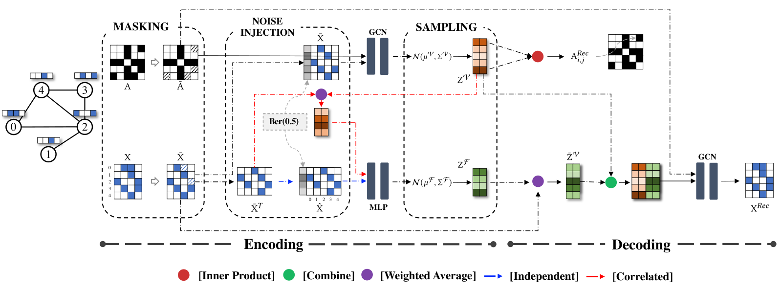
In this section, we present our model SeeGera. Different from SIG-VAE that uses node embeddings only, SeeGera further generates feature embeddings to capture the rich semantic information on node features, which can be used to enhance feature reconstruction. Specifically, we consider two cases in the encoder when generating node and feature embeddings: (1) they are independent; (2) they are correlated. After that, in the decoder part, we utilize GNNs to reconstruct node features based on both node and feature embeddings. Finally, we show how structure/feature masking can be integrated with the hierarchical variational framework and gives the optimization techniques. The overall framework of SeeGera is summarized in Figure 1.
4.1. Variational lower bound
In VI, given a graph with an adjacency matrix and a feature matrix , we approximate the true posterior with a variational distribution , where and are variational parameters. To capture more complex posteriors that go beyond the exponential family, we adopt the hierarchical variational framework in SIVI and assume
| (3) |
where and are parameters of mixing distributions. We marginalize and out and derive
| (4) |
We maximize the log-likelihood of observations and , and use Jensen’s inequality to get
| (5) |
where is ELBO and
| (6) |
is the marginal distribution over and . Since is often intractable, the Monte Carlo estimation of ELBO could be prohibited. To address the problem, we first take the mean-field assumption:
| (7) |
and substitute Eq. 7 into Eq. 6 to get:
| (8) |
From Eq. 8, we see that and are independent. Then we derive a lower bound for the ELBO based on Eq. 8:
| (9) |
Details on the derivation of Equation 9 are deferred to Appendix E. In , and are required to be explicit and have analytic density function, while and could be implicit but have to be convenient to be sampled from. Directly optimizing by Monte Carlo Estimation is much easier.
However, in practice, nodes and their features are highly correlated. On the one hand, node embeddings are generated based on features. On the other hand, the semantic information of features are directly reflected by nodes. Therefore, the independence between and in Equation 8 is inappropriate. To tackle the issue, we modify Eq. 7 into:
| (10) |
which explicitly characterizes the dependence between variational parameters and . In this way, , which shows that and are correlated. Then we can derive another lower bound for the ELBO in Equation 5:
| (11) |
4.2. Encoder
In the encoder, we generate and from observations and . We next show how to generate and according to whether they are independent or not.
[ and are independent]. To generate , we assume that , where and is multivariate Gaussian distribution with mean and diagonal co-variance matrix . Since and are random variables, we draw them by injecting noise into a GNN model:
| (12) |
where is the concatenation function and is a GNN model. Note that is random noise sampled from distribution , whose row size should be the same as . The injected noise enables the uncertainty propagation between neighboring nodes in the GNN layer, which drives the outputs of the GNN to be random variables rather than deterministic values. Similarly, for , we assume with . To infer and , we use a MLP model:
| (13) |
Note that and the -th row can be considered as the feature vector of feature . The random noise drawn from injects uncertainty to the matrix , which models and as random variables.
[ and are correlated]. We also assume and follow Gaussian distribution and use the same method as in Equation 12 to generate . However, to capture the dependence between and 22 2 Here, we denote and , respectively. in Equation 10, we compute for feature based on node embeddings. Specifically, since the rich semantic information of each feature is directly reflected by values of nodes in the feature, we take the feature vector as the weight vector over all the nodes, and compute:
| (14) |
In this way, is derived from node embeddings. Since and are random variables, and will also be random variables.
4.3. Decoder
In the decoder, we aim to reconstruct both edges and features in the given graph. The generative process is described as follows.
First, for each node and each feature , we draw 33 3 When and are independent, we draw and .. Second, for each edge in the adjacency matrix , draw . Here, denotes Bernoulli distribution and is the probability for the existence of edge . We implement simply by inner product as: , where is the sigmoid function. Third, for each attribute in the attribute matrix , draw . Here, are functions of and .
We next introduce how to compute and . Since contains rich semantic information on feature , the affinity between and can provide fine-grained knowledge for feature reconstruction. Given a node , to capture its affinities with all the features, the attention mechanism (Vaswani et al. 2017) can be applied on node and feature embeddings. However, this will increase the time complexity of the model. For simplicity, we directly use the feature vector of as the weight vector and calculate the weighted average over all the feature embeddings:
| (15) |
Compared with , contains more details on how each feature can be reconstructed. After that, we combine and to get:
| (16) |
In our experiments, we set the COMBINE function to be CONCAT. Finally, the updated is taken as input and fed into a GNN model to learn parameters w.r.t. node :
| (17) |
where is a GNN model.
4.4. Masking
To further improve the model generalizability, we introduce the masking mechanism in SeeGera by adding an additional layer to the hierarchical variational framework. Specifically, we transform Equation 6 into:
| (18) |
From the above equation, we see that in addition to and , the integration is performed over a new variable and a probability function . Here, denotes a new graph and is the graph augmentation probability function. The equation can lead to a new variational lower bound for the ELBO, but it is more difficult to optimize compared with and . To tackle the issue, we can first perform graph augmentation and generate a perturbed graph . After that, based on , node and feature embeddings are learned based on or . We repeat the above process until convergence. Although graph augmentation can include more operations than masking, we mainly focus on structure/feature masking in this paper, because masking is beneficial for node classification (Hou et al. 2022).
4.5. Optimization
In Section 4.1, we have derived two lower bounds and for the ELBO, according to whether and are independent. For notation brevity, we use to overload both and . However, directly optimizing could lead to the degeneracy problem (Yin and Zhou 2018) that , and might converge to a point mass density, which degenerates SIVI to the vanilla VI. To address the problem, we can regularize by :
Note that satisfies (1) ; (2) if and only if or degenerates to a point mass density. According to (Yin and Zhou 2018), is an asymptotically exact surrogate ELBO that satisfies and . Maximizing with derives positive and could drive away from degeneracy. Moreover, importance reweighting (Burda et al. 2015) can be further introduced to tighten by drawing samples from . The objective can be formulated as
| (19) |
where
Then we take as the surrogate ELBO and use stochastic gradient ascent to optimize it. Note that and treats differently for . Finally, we summarize the pseudocodes of SeeGera in Algorithm 1 (see Appendix B).
[Complexity analysis] The major time complexity in the encoder comes from GNN and MLP. Suppose we use GCN as the GNN model. Since the adjacency matrix is generally sparse, let be the average number of non-zero entries in each row of the adjacency matrix. Let be the number of features and be the embedding dimension. Further, we denote and as the dimensions of injected noise to the GCN and MLP, respectively. Then, the time complexities for GCN and MLP are and , respectively. In the decoder, suppose we still adopt GCN as the GNN model. Then the time complexities for reconstructing links and features are and , respectively. As suggested by (Kipf and Welling 2016), we can down-sample the number of nonexistent edges in the graph to reduce the time complexity for recovering links.
5. Experiment
In this section we comprehensively evaluate the quality of node embeddings learned by SeeGera. We mainly study four research questions:
(RQ1) How does SeeGera perform in the link prediction task?
(RQ2) Can SeeGera effectively predict node attributes?
(RQ3) While SeeGera is an unsupervised learning method, can it perform well when generalized to the node classification task?
(RQ4) How does structure/feature masking influence the performance of SeeGera?
5.1. Datasets and Baselines
To answer the above four questions, we conduct extensive experiments on seven public datasets: Cora, Citeseer, Pubmed, Coauthor CS, Coauthor Physics, Amazon Computer and Amazon Photo. Detailed descriptions and statistics on these datasets are provided in Appendix A. We also compare SeeGera with 9 other SOTA baselines, which can be categorized into two groups:
[Generative graph SSL methods]. This group of methods are based on GAE/VGAE and aim to reconstruct links and/or features, including SIG-VAE (Hasanzadeh et al. 2019), CAN (Meng et al. 2019), GATE (Salehi and Davulcu 2019) and GraphMAE (Hou et al. 2022). Note that GraphMAE is the SOTA generative graph SSL model.
[Graph contrastive learning methods]. Models in this type construct positive (and negative) pairs for contrast to learn node representations, including DGI (Velickovic et al. 2019), MVGRL (Hassani and Khasahmadi 2020), GRACE (Zhu et al. 2020), GCA (Zhu et al. 2021b) and CCA-SSG (Zhang et al. 2021).
Further, for more implementation details, see Appendix D.
| Metrics | Method | Cora | Citeseer | Pubmed | Photo | Computer | CS | Physics |
|---|---|---|---|---|---|---|---|---|
| AUC | DGI | |||||||
| MVGRL | OOM | |||||||
| GRACE | ||||||||
| GCA | ||||||||
| CCA-SSG | ||||||||
| CAN | ||||||||
| SIG-VAE | ||||||||
| GraphMAE | ||||||||
| SeeGera-v1 | ||||||||
| SeeGera-v2 | ||||||||
| SeeGera-v3 | ||||||||
| AP | DGI | |||||||
| MVGRL | OOM | |||||||
| GRACE | ||||||||
| GCA | ||||||||
| CCA-SSG | ||||||||
| CAN | ||||||||
| SIG-VAE | ||||||||
| GraphMAE | ||||||||
| SeeGera-v1 | ||||||||
| SeeGera-v2 | ||||||||
| SeeGera-v3 |
| Method | Cora | Citeseer | Pubmed | Photo | Computer | CS | Physics |
|---|---|---|---|---|---|---|---|
| CAN | - | - | - | - | - | ||
| GATE | OOM | ||||||
| GraphMAE | |||||||
| SeeGera-v1 | |||||||
| SeeGera-v2 | |||||||
| SeeGera-v3 |
| Method | Cora | Citeseer | Pubmed | Photo | Computer | CS | Physics |
|---|---|---|---|---|---|---|---|
| DGI | |||||||
| MVGRL | |||||||
| GRACE | |||||||
| CCA-SSG | |||||||
| GraphMAE | |||||||
| SeeGera-v1 | |||||||
| SeeGera-v2 | |||||||
| SeeGera-v3 |
5.2. Link Prediction (RQ1)
Link prediction is a typical unsupervised learning task for graph analysis, which aims to predict whether an edge exists between two nodes or not. We compare SeeGera with 8 other SOTA baselines, including GCL models: DGI (Velickovic et al. 2019), MVGRL (Hassani and Khasahmadi 2020), GRACE (Zhu et al. 2020), GCA (Zhu et al. 2021b), CCA-SSG (Zhang et al. 2021), and the generative graph SSL methods: CAN (Meng et al. 2019), SIG-VAE (Hasanzadeh et al. 2019), GraphMAE (Hou et al. 2022). For our proposed method SeeGera, we put forward three versions. Specifically, SeeGera-v1 assumes the independence between and and optimizes , while SeeGera-v2 captures the correlations between them and optimizes . Further, SeeGera-v3 upgrades SeeGera-v2 by adding the masking mechanism.
To evaluate the model performance, we construct the validation/test set by randomly selecting edges in the original graph as positive samples and an equal number of nonexistent edges as negative samples. After the removal of these selected edges, we train all the models on the resulting graph with the remaining edges. We use two commonly used metrics, the area under the ROC curve (AUC) and the average precision (AP), to report the model performance. For both metrics, a larger value indicates a better performance. We use the validation set for hyper-parameter tuning and early stopping with a patience of 100, i.e., we stop training if both metric scores on the validation set do not increase for 100 consecutive epochs. Similar as in (Kipf and Welling 2016), the predicted probability of an edge between nodes and is calculated by , where and is the sigmoid function. For each method, we run experiments 10 times and report the average results on the test set. Table 1 summarizes the results across all the datasets. From the table, we have the following observations:
(1) The generative graph SSL methods except GraphMAE generally perform better than GCL methods. This is because these methods learn to reconstruct links in the objective. For GraphMAE, it only reconstructs features, which explains its poor performance.
(2) While SeeGera is based on SIG-VAE, it achieves better performance. This demonstrates the importance of feature reconstruction and structure/feature masking.
(3) Although CAN co-embeds both nodes and features, it still performs not very well, due to the independence assumption between node and feature embeddings. Further, it uses linear decoder for feature reconstruction, which restricts the model’s effectiveness.
(4) SeeGera significantly outperforms other competitors across all the datasets, which indicates the superiority of generative VGAE model in graph representation learning. In particular, the consistent outperformance of SeeGera-v2 over SeeGera-v1 verifies the importance of capturing the correlations between node and feature embeddings. Further, the improvement of SeeGera-v3 over SeeGera-v2 shows the necessity of structure/feature masking.
5.3. Attribute Inference (RQ2)
Attribute inference is a task that predicts values of missing node attributes. Similar as in link prediction, we hide a certain percentage of node features and train on the rest. To construct the training/validation/test set, we randomly select node features. The validation set is used for hyper-parameter tuning and early stopping with a patience of 100 epoches. We take the Mean Squared Error (MSE) as the evaluation metric. The smaller the value, the better the performance. In this task, we compare SeeGera with generative graph SSL methods that reconstruct features in their decoders, including CAN (Park et al. 2019), GATE (Salehi and Davulcu 2019) and GraphMAE (Hou et al. 2022). For GCL models and other generative graph SSL methods that recover links only, they cannot be easily adapted to the task, so we do not take them as baselines. For each method, we run experiments 10 times and report the average results in Table 2. For Cora and Citeseer, we normalize node features for fair comparison, so CAN cannot be applied. From the table, while CAN, GATE and GraphMAE can perform well on some datasets, they cannot consistently provide excellent performance. For example, GraphMAE achieves the best result on Cora, but it performs very poorly on Citeseer. Further, SeeGera-v3 outperforms other competitors on 5 out of 7 datasets. This shows the effectiveness of our proposed feature reconstruction method and also the masking mechanism. We also notice that, in all cases, SeeGera-v2 achieves better performance than SeeGera-v1, which again verifies the necessity of capturing correlations between node and feature embeddings.
5.4. Node Classification (RQ3)
To further study SeeGera, we generalize learned embeddings to the node classification task. After node embeddings are trained on the entire graph, we train an additional classifier. Here, we employ Logistic Regression as the classifier. For Cora, Citeseer and Pubmed, we use the public split for evaluation, where each class has fixed 20 nodes for training, another fixed 500 nodes and 1000 nodes for validation and testing, respectively. For other datasets, we randomly split the nodes into 10%/10%/80% training/validation/test sets. We use classification accuracy as the metric to evaluate the model performance. Since GCL methods have been shown to perform well in classification tasks, we compare SeeGera with 4 state-of-the-arts, including DGI, MVGRL, GRACE and CCA-SSA. We also take the recently proposed generative model GraphMAE as baseline, because it bridges the gap between generative graph SSL models and GCL methods in terms of classification tasks. Table 3 summarizes the classification results on all the datasets. From the table, we see that CCA-SSG, GraphMAE and SeeGera lead other competitors and they almost tie. This shows that SeeGera achieves comparable performance with the state-of-the-art methods in the node classification task. Further, with the significant advantage in link prediction and attribute inference tasks, we conclude that SeeGera, a VGAE-based graph SSL method, can generate versatile node representations that can be widely used in various downstream tasks.
5.5. Parameter Analysis (RQ4)
We end this section with a sensitivity analysis on the key hyperparameters in SeeGera, i.e., the structure masking rate and the feature masking rate . Specifically, we explore the stability of SeeGera w.r.t. the perturbation of and . We conduct experiments on the link prediction task by varying these parameters from 0 to 0.5, and keeping others fixed. Figure 2 illustrates the AUC and AP scores of SeeGera-v3 under different and values on Cora and Citeseer. From the figure, we see that SeeGera-v3 can give very stable performance over a wide range of and values, as shown by the plateau in the figure. This demonstrates the insensitivity of SeeGera w.r.t. these two hyper-parameters.
6. Conclusions
We studied generative graph SSL in this paper and proposed SeeGera, which enhances the family of VGAE on graph representation learning. Specifically, SeeGera adopts the hierarchical variational framework in SIG-VAE and mainly focuses on feature reconstruction and structure/feature masking. On the one hand, SeeGera co-embeds both nodes and features in the encoder and computes their embeddings by assuming they are independent and correlated, respectively. After that, feature embeddings that contain rich semantic information on features are combined with node embeddings to provide more fine-grained information for feature reconstruction in the decoder. On the other hand, we injected the masking mechanism into SeeGera by adding an additional layer to the hierarchical variational framework. We conducted extensive experiments to evaluate the performance of SeeGera. The results show that SeeGera significantly outperforms other competitors in link prediction and attribute inference, and achieves comparable results with them in node classification. This further verifies the power of generative graph SSL methods in graph representation learning.
Acknowledgement
This work is supported by Shanghai Pujiang Talent Program No. 21PJ1402900, Shanghai Science and Technology Committee General Program No. 22ZR1419900 and National Natural Science Foundation of China No. 62202172.
References
- (1)
- Burda et al. (2015) Yuri Burda, Roger Grosse, and Ruslan Salakhutdinov. 2015. Importance weighted autoencoders. arXiv preprint arXiv:1509.00519 (2015).
- Devlin et al. (2018) Jacob Devlin, Ming-Wei Chang, Kenton Lee, and Kristina Toutanova. 2018. Bert: Pre-training of deep bidirectional transformers for language understanding. arXiv preprint arXiv:1810.04805 (2018).
- Garcia Duran and Niepert (2017) Alberto Garcia Duran and Mathias Niepert. 2017. Learning graph representations with embedding propagation. Advances in neural information processing systems 30 (2017).
- Hasanzadeh et al. (2019) Arman Hasanzadeh, Ehsan Hajiramezanali, Krishna Narayanan, Nick Duffield, Mingyuan Zhou, and Xiaoning Qian. 2019. Semi-implicit graph variational auto-encoders. In NeurIPS. 10711–10722.
- Hassani and Khasahmadi (2020) Kaveh Hassani and Amir Hosein Khasahmadi. 2020. Contrastive multi-view representation learning on graphs. In International Conference on Machine Learning. PMLR, 4116–4126.
- He et al. (2020) Kaiming He, Haoqi Fan, Yuxin Wu, Saining Xie, and Ross Girshick. 2020. Momentum contrast for unsupervised visual representation learning. In Proceedings of the IEEE/CVF conference on computer vision and pattern recognition. 9729–9738.
- Hou et al. (2022) Zhenyu Hou, Xiao Liu, Yuxiao Dong, Chunjie Wang, Jie Tang, et al. 2022. GraphMAE: Self-Supervised Masked Graph Autoencoders. arXiv preprint arXiv:2205.10803 (2022).
- Hu et al. (2019) Weihua Hu, Bowen Liu, Joseph Gomes, Marinka Zitnik, Percy Liang, Vijay Pande, and Jure Leskovec. 2019. Strategies for pre-training graph neural networks. arXiv preprint arXiv:1905.12265 (2019).
- Hu et al. (2020) Ziniu Hu, Yuxiao Dong, Kuansan Wang, Kai-Wei Chang, and Yizhou Sun. 2020. Gpt-gnn: Generative pre-training of graph neural networks. In Proceedings of the 26th ACM SIGKDD International Conference on Knowledge Discovery & Data Mining. 1857–1867.
- Jiao et al. (2020) Yizhu Jiao, Yun Xiong, Jiawei Zhang, Yao Zhang, Tianqi Zhang, and Yangyong Zhu. 2020. Sub-graph contrast for scalable self-supervised graph representation learning. In ICDM. IEEE, 222–231.
- Kingma and Welling (2014) Diederik P Kingma and Max Welling. 2014. Auto-encoding variational bayes. In ICLR.
- Kipf and Welling (2016) Thomas N Kipf and Max Welling. 2016. Variational graph auto-encoders. arXiv preprint arXiv:1611.07308 (2016).
- Kipf and Welling (2017) Thomas N Kipf and Max Welling. 2017. Semi-supervised classification with graph convolutional networks. In ICLR.
- Li et al. (2022) Alexander C Li, Alexei A Efros, and Deepak Pathak. 2022. Understanding Collapse in Non-Contrastive Learning. arXiv preprint arXiv:2209.15007 (2022).
- Liu et al. (2022) Yixin Liu, Ming Jin, Shirui Pan, Chuan Zhou, Yu Zheng, Feng Xia, and Philip Yu. 2022. Graph self-supervised learning: A survey. IEEE Transactions on Knowledge and Data Engineering (2022).
- Liu et al. (2021) Yixin Liu, Zhao Li, Shirui Pan, Chen Gong, Chuan Zhou, and George Karypis. 2021. Anomaly detection on attributed networks via contrastive self-supervised learning. TNNLS 33, 6 (2021), 2378–2392.
- McAuley et al. (2015) Julian McAuley, Christopher Targett, Qinfeng Shi, and Anton Van Den Hengel. 2015. Image-based recommendations on styles and substitutes. In SIGIR. 43–52.
- Meng et al. (2019) Zaiqiao Meng, Shangsong Liang, Hongyan Bao, and Xiangliang Zhang. 2019. Co-embedding attributed networks. In WSDM. 393–401.
- Pan et al. (2018) Shirui Pan, Ruiqi Hu, Guodong Long, Jing Jiang, Lina Yao, and Chengqi Zhang. 2018. Adversarially regularized graph autoencoder for graph embedding. In IJCAI. 2609–2615.
- Park et al. (2019) Jiwoong Park, Minsik Lee, Hyung Jin Chang, Kyuewang Lee, and Jin Young Choi. 2019. Symmetric graph convolutional autoencoder for unsupervised graph representation learning. In Proceedings of the IEEE/CVF International Conference on Computer Vision. 6519–6528.
- Qiu et al. (2020) Jiezhong Qiu, Qibin Chen, Yuxiao Dong, Jing Zhang, Hongxia Yang, Ming Ding, Kuansan Wang, and Jie Tang. 2020. Gcc: Graph contrastive coding for graph neural network pre-training. In Proceedings of the 26th ACM SIGKDD International Conference on Knowledge Discovery & Data Mining. 1150–1160.
- Rainforth et al. (2018) Tom Rainforth, Adam R Kosiorek, Tuan Anh Le, Chris J Maddison, Maximilian Igl, Frank Wood, and Yee Whye Teh. 2018. Tighter variational bounds are not necessarily better. In ICML. 4274–4282.
- Salehi and Davulcu (2019) Amin Salehi and Hasan Davulcu. 2019. Graph attention auto-encoders. arXiv preprint arXiv:1905.10715 (2019).
- Sinha et al. (2015) Arnab Sinha, Zhihong Shen, Yang Song, Hao Ma, Darrin Eide, Bo-June Hsu, and Kuansan Wang. 2015. An overview of microsoft academic service (mas) and applications. In Proceedings of the 24th international conference on world wide web. 243–246.
- Sønderby et al. (2016) Casper Kaae Sønderby, Tapani Raiko, Lars Maaløe, Søren Kaae Sønderby, and Ole Winther. 2016. Ladder variational autoencoders. In NeurIPS. 3738–3746.
- Sun et al. (2019) Fan-Yun Sun, Jordan Hoffmann, Vikas Verma, and Jian Tang. 2019. Infograph: Unsupervised and semi-supervised graph-level representation learning via mutual information maximization. arXiv preprint arXiv:1908.01000 (2019).
- Thakoor et al. (2021) Shantanu Thakoor, Corentin Tallec, Mohammad Gheshlaghi Azar, Mehdi Azabou, Eva L Dyer, Remi Munos, Petar Veličković, and Michal Valko. 2021. Large-scale representation learning on graphs via bootstrapping. arXiv preprint arXiv:2102.06514 (2021).
- Vaswani et al. (2017) Ashish Vaswani, Noam Shazeer, Niki Parmar, Jakob Uszkoreit, Llion Jones, Aidan N Gomez, Łukasz Kaiser, and Illia Polosukhin. 2017. Attention is all you need, Vol. 30.
- Velickovic et al. (2019) Petar Velickovic, William Fedus, William L Hamilton, Pietro Liò, Yoshua Bengio, and R Devon Hjelm. 2019. Deep Graph Infomax. ICLR (Poster) 2, 3 (2019), 4.
- Wang et al. (2017) Chun Wang, Shirui Pan, Guodong Long, Xingquan Zhu, and Jing Jiang. 2017. Mgae: Marginalized graph autoencoder for graph clustering. In Proceedings of the 2017 ACM on Conference on Information and Knowledge Management. 889–898.
- Xu et al. (2021) Minghao Xu, Hang Wang, Bingbing Ni, Hongyu Guo, and Jian Tang. 2021. Self-supervised graph-level representation learning with local and global structure. In International Conference on Machine Learning. PMLR, 11548–11558.
- Yin and Zhou (2018) Mingzhang Yin and Mingyuan Zhou. 2018. Semi-Implicit Variational Inference. In ICML. 5660–5669.
- You et al. (2018a) Jiaxuan You, Bowen Liu, Zhitao Ying, Vijay Pande, and Jure Leskovec. 2018a. Graph convolutional policy network for goal-directed molecular graph generation. Advances in neural information processing systems 31 (2018).
- You et al. (2018b) Jiaxuan You, Rex Ying, Xiang Ren, William Hamilton, and Jure Leskovec. 2018b. Graphrnn: Generating realistic graphs with deep auto-regressive models. In International conference on machine learning. PMLR, 5708–5717.
- You et al. (2020a) Yuning You, Tianlong Chen, Yongduo Sui, Ting Chen, Zhangyang Wang, and Yang Shen. 2020a. Graph contrastive learning with augmentations. Advances in Neural Information Processing Systems 33 (2020), 5812–5823.
- You et al. (2020b) Yuning You, Tianlong Chen, Zhangyang Wang, and Yang Shen. 2020b. When does self-supervision help graph convolutional networks?. In international conference on machine learning. PMLR, 10871–10880.
- Zhang et al. (2021) Hengrui Zhang, Qitian Wu, Junchi Yan, David Wipf, and Philip S Yu. 2021. From canonical correlation analysis to self-supervised graph neural networks. Advances in Neural Information Processing Systems 34 (2021), 76–89.
- Zhang et al. (2020) Jiawei Zhang, Haopeng Zhang, Congying Xia, and Li Sun. 2020. Graph-bert: Only attention is needed for learning graph representations. arXiv preprint arXiv:2001.05140 (2020).
- Zhou et al. (2020) Sheng Zhou, Xin Wang, Jiajun Bu, Martin Ester, Pinggang Yu, Jiawei Chen, Qihao Shi, and Can Wang. 2020. DGE: Deep Generative Network Embedding Based on Commonality and Individuality. In AAAI.
- Zhu et al. (2021a) Yanqiao Zhu, Yichen Xu, Qiang Liu, and Shu Wu. 2021a. An empirical study of graph contrastive learning. arXiv preprint arXiv:2109.01116 (2021).
- Zhu et al. (2020) Yanqiao Zhu, Yichen Xu, Feng Yu, Qiang Liu, Shu Wu, and Liang Wang. 2020. Deep graph contrastive representation learning. arXiv preprint arXiv:2006.04131 (2020).
- Zhu et al. (2021b) Yanqiao Zhu, Yichen Xu, Feng Yu, Qiang Liu, Shu Wu, and Liang Wang. 2021b. Graph contrastive learning with adaptive augmentation. In Proceedings of the Web Conference 2021. 2069–2080.
Appendix A Datasets
We use 7 public datasets which do not have license. We next briefly introduce them as follows.
Cora, Citeseer and Pubmed (Kipf and Welling 2017) are three citation networks, where nodes represent publications and edges are citation links. Features for each node are the keywords it contains. Each dimension in the feature vector indicates the presence of a keyword in the publication. Nodes in these datasets are associated with labels that describe research topics of publications.
Coauther CS and Coauther Physics are co-authorship graphs based on the Microsoft Academic Graph from the KDD Cup 2016 challenge (Sinha et al. 2015). In these datasets, nodes are authors and edges capture the co-authorship. Further, node features represent keywords in each author’s papers, and class labels indicate the study fields for authors.
Amazon Computer and Amazon Photo are extracted from the Amazon co-purchase graph (McAuley et al. 2015), where nodes represent goods and edges indicate that two goods are frequently bought together. Node features are bag-of-words encoded product reviews and class labels are the product categories. The statistics of these datasets are summarized in Table 4.
Appendix B Pseudocodes
This section summarizes the pseudocodes of SeeGera-v3 in Alg. 1.
| Datasets | #Nodes | #Edges | #Features | #Classes |
|---|---|---|---|---|
| Cora | ||||
| Citeseer | ||||
| Pubmed | ||||
| Coauthor CS | ||||
| Coauthor Physics | ||||
| Amazon Computer | ||||
| Coauthor Physics |
Appendix C Ablation study
We conduct an ablation study to investigate the main components in SeeGera. In particular, we have extensively compared SeeGera-v1, SeeGera-v2 and SeeGera-v3 in our experiments. The advantage of SeeGera-v2 over SeeGera-v1 shows the importance of capturing the correlations between node and feature embeddings. Also, the outperformance of SeeGera-v3 over SeeGera-v2 verifies the importance of the masking mechanism. Further, to show the effectiveness of our proposed feature reconstruction method, we remove feature embeddings in the encoder and feed only node embeddings into GCN in the decoder to reconstruct features. We call this variant SeeGera_nf (no feature embedding). Table 5 shows the results on attribute inference. We exclude SeeGera-v3 in the table, because it further uses the masking mechanism while others not. From the table, we see that both SeeGera-v1 and SeeGera-v2 outperform SeeGera_nf. This shows the importance of using both node and feature embeddings for feature reconstruction.
| Method | Cora | Citeseer | CS |
|---|---|---|---|
| SeeGera_nf | |||
| SeeGera-v1 | |||
| SeeGera-v2 |
Appendix D Implementation Details
We implemented SeeGera by PyTorch. The model is initialized by Glorot initialization and trained by Adam. We run the model for 3500 epochs on all the datasets. In particular, for the task of node classification, we further run the logistic regression classifier for 500 epochs. We adopt GCNs in both encoder and decoder for all the datasets except CS. For CS, we use MLPs to replace GNNs instead. We choose Bernoulli noise Ber(0.5) for both and , and set the noise dimension to 5 in all tasks. As suggested by (Sønderby et al. 2016), we use warm-up during the first 300 epochs to gradually impose the prior regularization terms and . For both priors and , we assume that they follow standard multivariate normal distributions. In the node classification task, most results of baselines are publicly available and we directly report these results from their original papers. For the results that are missing, we run the released codes by their authors and fine-tune the model hyper-parameters. In the link prediction and attribute inference tasks, since most baselines are not studied in these tasks, we run their released codes with fine-tuning. For fairness, we run all the experiments on a server with a single NVIDIA A100 GPU with 80G memory. For simplicity, we set in Eq. 19 for both SeeGera and SIG-VAE. One may further refer to (Rainforth et al. 2018) for better value selection. All the datasets and codes are provided at https://github.com/SeeGera/SeeGera. We provide the detailed hyper-parameter settings of SeeGera-v3 on different datasets in Tables 6- 8. All hyper-parameters are selected through small grid search, and the search space is provided as:
- •
Number of layers in the encoder : {1, 2, 3}
- •
Number of layers in the decoder : {1, 2, 3}
- •
Learning rate of SeeGera: {1e-3, 5e-3, 1e-2}
- •
Dropout of SeeGera: {0, 0.1, 0.3, 0.5, 0.7, 0.9}
- •
Weight decay of SeeGera: {5e-5, 1e-4, 5e-4, 1e-3}
- •
Structure masking rate : {0, 0.1, 0.2, 0.3, 0.4, 0.5}
- •
Feature masking rate : {0, 0.1, 0.2, 0.3, 0.4, 0.5}
- •
Learning rate of logistic regression: {1e-3, 5e-3, 1e-2}
- •
Dropout of logistic regression: {0, 0.1, 0.3, 0.5, 0.7, 0.9}
- •
Weight decay of logistic regression: {5e-5, 1e-4, 5e-4, 1e-3}
| Dataset | lr | dropout | wd | ||||
|---|---|---|---|---|---|---|---|
| Cora | 2 | 3 | 1e-3 | 0.3 | 5e-5 | 0.3 | 0.0 |
| Citeseer | 1 | 2 | 1e-3 | 0.0 | 1e-4 | 0.6 | 0.0 |
| Pubmed | 2 | 1 | 5e-3 | 0.5 | 0.0 | 0.3 | 0.1 |
| Photo | 1 | 1 | 5e-3 | 0.0 | 0.0 | 0.5 | 0.0 |
| Computer | 2 | 2 | 1e-3 | 0.0 | 0.0 | 0.4 | 0.0 |
| CS | 1 | 2 | 1e-3 | 0.0 | 0.0 | 0.5 | 0.5 |
| Physics | 2 | 2 | 1e-3 | 0.0 | 0.0 | 0.2 | 0.0 |
| Dataset | lr | dropout | wd | ||||
|---|---|---|---|---|---|---|---|
| Cora | 1 | 1 | 1e-3 | 0.1 | 5e-5 | 0.4 | 0.0 |
| Citeseer | 1 | 1 | 1e-3 | 0.0 | 0.0 | 0.3 | 0.0 |
| Pubmed | 2 | 2 | 1e-3 | 0.0 | 0.0 | 0.0 | 0.1 |
| Photo | 2 | 3 | 1e-3 | 0.0 | 0.0 | 0.3 | 0.0 |
| Computer | 2 | 3 | 1e-3 | 0.0 | 0.0 | 0.2 | 0.0 |
| CS | 1 | 3 | 1e-3 | 0.0 | 0.0 | 0.1 | 0.5 |
| Physics | 2 | 2 | 1e-3 | 0.0 | 0.0 | 0.0 | 0.0 |
| Dataset | SeeGera | Logistic Regression | ||||||||
|---|---|---|---|---|---|---|---|---|---|---|
| lr | dropout | wd | lr | dropout | wd | |||||
| Cora | 2 | 2 | 1e-3 | 0.3 | 1e-3 | 0.2 | 0.1 | 1e-3 | 0.9 | 1e-3 |
| Citeseer | 2 | 2 | 5e-3 | 0.3 | 5e-4 | 0.0 | 0.0 | 1e-3 | 0.9 | 0.0 |
| Pubmed | 2 | 1 | 5e-3 | 0.7 | 0.0 | 0.0 | 0.0 | 1e-3 | 0.3 | 0.0 |
| Photo | 1 | 2 | 1e-3 | 0.0 | 5e-4 | 0.5 | 0.5 | 5e-3 | 0.7 | 5e-5 |
| Computer | 1 | 3 | 5e-3 | 0.0 | 5e-4 | 0.0 | 0.0 | 5e-3 | 0.3 | 1e-4 |
| CS | 2 | 3 | 1e-2 | 0.1 | 1e-3 | 0.4 | 0.0 | 1e-2 | 0.0 | 1e-3 |
| Physics | 1 | 3 | 1e-2 | 0.0 | 0.0 | 0.0 | 0.0 | 1e-2 | 0.5 | 5e-5 |
Appendix E Variational lower bound
In this section, we show the derivation on the variational lower bounds in detail.
where is the KL divergence and we employ according to (Yin and Zhou 2018). To better understand , we decompose the joint distribution as
and expand to derive:
Here, and are encoders that generate embeddings of nodes and features, respectively; and are decoders that reconstruct links and features from learned embeddings. The first two terms in the equation correspond to the negative reconstruction loss for links and features, while the last two terms are regularizers that promote the closeness between variational distributions and prior distributions.
Similarly, we can expand as: