Convergence and Near-optimal Sampling for Multivariate Function Approximations in Irregular Domains via Vandermonde with Arnoldi
Abstract
Vandermonde matrices are usually exponentially ill-conditioned and often result in unstable approximations. In this paper, we introduce and analyze the multivariate Vandermonde with Arnoldi (V+A) method, which is based on least-squares approximation together with a Stieltjes orthogonalization process, for approximating continuous, multivariate functions on -dimensional irregular domains. The V+A method addresses the ill-conditioning of the Vandermonde approximation by creating a set of discrete orthogonal bases with respect to a discrete measure. The V+A method is simple and general, relying only on the domain’s sample points. This paper analyzes the sample complexity of the least-squares approximation that uses the V+A method. We show that, for a large class of domains, this approximation gives a well-conditioned and near-optimal -dimensional least-squares approximation using equispaced sample points or random sample points, independently of . We provide a comprehensive analysis of the error estimates and the rate of convergence of the least-squares approximation that uses the V+A method. Based on the multivariate V+A techniques, we propose a new variant of the weighted V+A least-squares algorithm that uses only sample points to achieve a near-optimal approximation. Our initial numerical results validate that the V+A least-squares approximation method provides well-conditioned and near-optimal approximations for multivariate functions on (irregular) domains. Additionally, the (weighted) least-squares approximation that uses the V+A method performs competitively with state-of-the-art orthogonalization techniques and can serve as a practical tool for selecting near-optimal distributions of sample points in irregular domains.
Keywords: least-squares, Vandermonde matrix, Arnoldi, polyval, polyfit, ill-conditioning, sample complexity, near-optimal sampling
1 Introduction and Overview of the Paper
Many problems in computational science call for the approximation of smooth, multivariate functions. In this paper, we consider the problem of approximating a multivariate continuous function of variables, where the domain may be irregular. Using Vandermonde matrices to fit polynomials is one of the most straightforward approaches. However, the Vandermonde matrix is usually exponentially ill-conditioned, even on standard domains such as an interval, unless the sample points are very carefully chosen [9, 27, 31]. Recently, in [11], the authors developed an orthogonalization framework that couples Vandermonde matrices with Arnoldi orthogonalization for univariate function approximations, known as the univariate Vandermonde with Arnoldi method (V+A).
In this paper, we extend the univariate V+A method to a multivariate version that can be used for -dimensional function approximations (). The multivariate V+A method is based on least-squares approximation coupled with a Stieltjes orthogonalization process, aimed at approximating continuous, multivariate functions on irregular -dimensional domains. This method establishes a set of discrete multivariate orthogonal bases with respect to a discrete measure.
There is extensive literature on -dimensional polynomial approximation algorithms that assume the function is defined over a hypercube domain containing the irregular domain [4, 5, 15]. These algorithms, commonly known as polynomial frame approximations, create an orthogonal basis in the hypercube domain. On the other hand, the V+A algorithm creates a discrete orthogonal basis directly in and effectively constructs a well-conditioned basis for the irregular domain . It is well-known that, even if we have a well-conditioned basis, least-squares approximations can still become inaccurate when the number of sample points (from a suboptimal distribution, e.g., equispaced points) is insufficient, such as when is close to the dimension of the approximation space . Poorly distributed sample points can also affect the quality of the solution. In some domains, polynomial frame approximations have provable bounds on the sample complexity; namely, the scaling between the dimension of the approximation space and the number of samples , which is sufficient to guarantee a well-conditioned and accurate approximation [2, 5, 15]. However, to the best of our knowledge, there appears to be no literature on the sample complexity of the V+A procedure.
A key theoretical contribution of this paper is to investigate how behaves as a function of such that the least-squares approximant converges to as the total degree of freedom in approximation . We show that, in a large number of domains (i.e., real intervals, convex domains, or finite unions of convex domains), the least-squares approximation using the V+A method gives a well-conditioned and accurate -dimensional approximation using equispaced sample points or random sample points. The sample complexity of the least-squares approximation using the V+A method is comparable to that of polynomial frame approximation [2, 4, 15]. However, since V+A only requires enough sample points such that the discrete orthogonal polynomials are nearly orthogonal in the whole/continuous domain of interest, it can, in some cases, provide an approximation of similar accuracy using fewer sample points. In addition, since the least-squares problem to be solved becomes well-conditioned, it requires no sophisticated analysis or algorithm to compute an accurate solution (in frame approximation, a remarkable result is that despite the ill-conditioning, one can find a near-optimal solution by finding a small-norm solution using the truncated SVD [2, 4]). Using results on sample complexity, we further prove that, under suitable sample distributions and domains, the least-squares approximation that uses the multivariate V+A method is near-optimal. Specifically, the th polynomial approximation obtained (referred to as the V+A approximant) converges to at a spectral rate with respect to for the total degree polynomial space, contingent upon the smoothness of in
In addition to theory, we provide numerical studies for the multivariate V+A method. Our preliminary numerical results indicate that the multivariate V+A method effectively tackles the ill-conditioning associated with the Vandermonde approximation. To our knowledge, the multivariate V+A algorithm introduced in [24] is implemented only for rational approximations on standard 1D or 2D domains. We extend the numerical applications of the multivariate V+A algorithm to include polynomial approximation on 2D (irregular domains) and higher-dimensional domains (). Our initial numerical results indicate that as increases, the V+A least-squares approximation provides a significantly more accurate approximation compared to the Vandermonde least-squares method for . In several papers [2, 3, 16, 30], the authors proved that an effective weighting can lead to the near-optimal scaling of . However, in past approaches [2], the QR factorization was used to orthogonalize the least-squares system. A key numerical contribution of this paper is that we propose a variant of the weighted least-squares algorithm that uses the multivariate V+A as the orthogonalization method (VA+Weight). This algorithm is stable with high probability and only takes sample points to give a near-optimal approximation. Due to the reduced sample density, VA+Weight also gives a lower online computational cost than the unweighted least-squares using the V+A method. Our initial numerical results confirm that VA+Weight performs competitively with state-of-the-art orthogonalization techniques for the Vandermonde matrix. Finding the optimal distribution of sample points in a high-dimensional irregular domain is an open question in the literature [14]. Our preliminary numerical results highlight that VA+Weight is a practical tool for selecting the near-optimal distribution of sample points for the irregular domains considered in this paper.
The paper is arranged as follows. In Section 2, we introduce the Arnoldi orthogonalization procedure in the least squares approximation setup, presenting the univariate V+A algorithm along with three examples of its numerical applications. In Section 3, we extend the univariate V+A algorithm to higher dimensions. We compare the multivariate V+A method with other techniques and showcase its effectiveness through five examples of numerical applications in function approximation within -dimensional (irregular) domains (). Section 4 gives our main theoretical result on sample complexity and convergence rate of least squares approximation using the V+A algorithm on general -dimensional domains. In Section 5, we give the weighted V+A least-squares algorithm, VA+Weight, which takes only sample points to give a near-optimal approximation.
1.1 Related Work
The idea of orthogonalizing monomials and combining Vandermonde with Arnoldi is not completely new. Past emphasis has been on constructing continuous orthogonal polynomials on a continuous domain. The purpose of the orthogonalization is to obtain the orthogonal polynomial itself [21, 22]. However, V+A, also known as Stieltjes orthogonalization [18, 34], is a versatile method that can dramatically improve the stability of polynomial approximation [11]. The purpose of the orthogonalization is to improve the numerical stability of the least-squares system.
The multivariate version of V+A was first discussed by Hokanson [24], who applies V+A to the Sanathanan-Koerner iteration in rational approximation problems. See also [7]. In these studies, the multivariate V+A is used for rational approximations on standard domains. Applying the V+A algorithm to approximate multivariate functions on irregular domains appears not to have been considered in the literature.
It is worth noting that V+A also has numerous applications beyond polynomial approximation. For instance, it can be used in the ‘lightning’ solver [20], a state-of-the-art PDE solver that solves Laplace’s equation on an irregular domain using rational functions with fixed poles. We also combine V+A with Lawson’s algorithm [28] to improve the accuracy of the approximation. We refer to this algorithm as VA+Lawson. VA+Lawson attempts to find the best polynomial approximation11 1 The best approximation is defined in Remark 3.2 (3). in difficult domains (for instance, disjoint complex domains). VA+Lawson is also a powerful tool for finding the minimal polynomial for the GMRES algorithms and power iterations in irregular complex domains.
2 Univariate Vandermonde with Arnoldi
Polynomial approximation of an unknown function by fitting a polynomial to a set of sample points from the domain is a classic problem. The interpolation and least-squares methods are two methods to solve this type of problem [30, 32]. We start with the simplest 1D polynomial approximation problem in this section.
Let be a bounded domain, a set of distinct sample points and a continuous function which gives a value at each sample point. Let represent the space of univariate () polynomials with the highest order , and denotes the total degrees of freedom. We aim to find a th degree polynomial approximation, , such that
| (1) |
We can write where are the monomial coefficients to be determined. The equation (1) can be formulated as a Vandermonde least-squares problem
| (2) |
Using the pseudoinverse, we can write the solution as where is an Vandermonde matrix with the th entry for , , , and . Since the sample points are distinct, is full rank and thus the solution exists and is unique. If , we have an interpolation problem, and is a square matrix. The solution is given by . If , is a tall rectangular matrix and we have a least-squares problem with normal equation .
The least-squares problem (2) has the same solution as the normal equation If is well-conditioned, the least squares problem can be solved by the normal equation. However, if is moderately (or highly) ill-conditioned, since the condition number of is the square of the condition number of , the conditioning of the normal equation significantly worsens. In this paper, unless otherwise stated, we focus on the least-squares problem (2) and assume that .
Ideally, we can find the coefficients of the polynomial approximation by solving the least-squares problem (2). However, the Vandermonde matrices are well known to be exponentially ill-conditioned [27] (unless the nodes are uniformly distributed on the unit circle). This creates instability in solving the Vandermonde system and makes a moderately high degree Vandermonde approximation inaccurate. The ill-conditioning of the Vandermonde matrix is due to the non-orthogonal nature of the monomial basis. A potential solution to the ill-conditioning is to treat the monomial basis as a Krylov subspace sequence, such that
| (3) |
where , , and . Based on this observation, in V+A we apply Arnoldi orthogonalization to the Krylov space . The Krylov space is orthogonalized by the decomposition where is the matrix with columns and is the same matrix without the final column. By the Arnoldi process, we transform the ill-conditioned Vandermonde system into an optimally conditioned system22 2 The condition number of is .,
| (4) |
and is defined as before.
| (Discrete Orthogonal Polynomials) |
is known as a set of discrete orthogonal polynomials or a discrete orthogonal basis. denotes the coefficient vector related to the discrete orthogonal polynomials, such that . By construction, the discrete orthogonal basis spans the polynomial space . We say that satisfies discrete orthogonality w.r.t. , if
| (Discrete Orthogonality) |
where denotes the Kronecker delta. On real intervals, the discrete orthogonal polynomials are known to satisfy many algebraic properties analogous to those of the continuous orthogonal polynomials [21, 40].
2.1 Algorithm for Vandermonde with Arnoldi
The Arnoldi algorithm, originally applied to finding eigenvalues, uses the modified Gram-Schmidt process to produce a sequence of orthogonal vectors. The orthogonal columns are obtained by the following recurrence formula
| (5) |
where and . Note that for all with and for . The scaling of ensures that the Euclidean norm of the V+A solution, , is relatively constant as the number of sample points increases. are the coefficients of the recurrence formula and also denote the th entries of the matrix . By orthogonality, is a lower Hessenberg matrix. For real sample points, , is tridiagonal and the Arnoldi algorithm is equivalent to the Lanczos algorithm.
In the Vandermonde least-squares system (2), we construct the full matrix and solve the poorly conditioned linear system. In V+A, however, we form the matrix column by column, orthogonalizing each new column against all previous columns using the Arnoldi algorithm. Thus, the Arnoldi process gives us an optimally-conditioned least-squares problem (i.e., the condition number of , ) . The solution for the least-squares system exists,
| (6) |
where the factor comes from the column scaling of such that . Note that the solution of the Vandermonde system, , and the solution of the V+A system, , are related by . In MATLAB, can be obtained either by (6) or by the backslash command. The backslash command invokes the QR factorization for the least-squares problem and the Gaussian elimination for the interpolation problem (when ). For improved accuracy, we choose to obtain using the backslash command for the extra round of orthogonalization [11].
Once the vector of coefficients is obtained, the least-squares approximant can be evaluated at a different set of points . The entries of the th column of are the coefficients used in the recursion formula of the discrete orthogonal polynomial, such that
| (7) |
In the polynomial evaluation process, we use the same recursion formula as in (7) but apply it on a different set of points, , such that
| (8) |
with and is given a priori by the Arnoldi process. The polynomials are evaluated at by , where and is obtained a priori by the Arnoldi process. The th entry of represents for . Note that the columns of are in general approximately orthogonal, but not orthogonal. To test the validity of the least-squares approximant, we usually evaluate the polynomial approximant on a much finer mesh with and compare the evaluated values with . We assess the error of the approximant using this method by computing the maximum absolute value at the evaluation points, .
Algorithm and Costs: The univariate V+A fitting and evaluation is implemented in [11] using less than 15 lines of MATLAB code. We made slight variations to the code to improve their efficiency. We provide the algorithm in Algorithms 1 and 2. Instead of using modified Gram-Schmidt (MGS), we use the classical Gram-Schmidt (CGS) repeated twice, as it gives excellent orthogonality and speed. Doing CGS twice creates a discrete orthogonal basis that satisfies , where is the unit roundoff. This is better than MGS, and a good enough bound for polynomial approximation problems which usually have dimensions of and . More details on the univariate V+A algorithm can be found in [11].
Remark 2.1.
The notations in the algorithms in this paper represent the following.
- •
refers to all the elements in the th column of the matrix .
- •
refers to all the elements from the first to the th element in the th row of the matrix .
- •
refers to all the elements from the first to the th column of the matrix .
Output: , the coefficient of the approximation .
Initialize and as zero matrices; Set as a matrix of ones.
For
For (Carry out classical Gram-Schmidt twice)
end
;
end
Solve the least-squares problem by MATLAB backslash command.
For
end
2.2 Applications and Numerical Examples for Univariate V+A
In the first paper on V+A [11], several applications of the univariate V+A method are provided, including interpolation at Chebyshev points, least-squares approximation on two intervals, Fourier extension, Laplace equation, and conformal mapping. In addition to these applications presented in [11], we explore three additional examples of V+A least-squares polynomial approximations.
Example 2.1.
(Disjoint Domain) Approximating using equispaced sample points in a disjoint domain . This example challenges the algorithm’s ability to handle a disjoint domain. We compare the V+A method to the Vandermonde method in the left plot of Figure 1. Initially, the two approximations give the same error. However, the Vandermonde system has an error stagnating at for due to ill-conditioning of , while the V+A method gives an error reduction down to as increases.
Example 2.2.
(Non-Smooth Function) Approximating in using random sample points. This example tests the algorithm on approximating a non-smooth function with random uniform sample points. Similar to Example 1, V+A also yields a much better approximation than the Vandermonde approximation (the middle plot of Figure 1). The error for V+A is also in line with the error of the best polynomial approximation () [33].
Example 2.3.
(Infinite Domain) Approximating in using logarithmic equispaced points. The logarithmic equispaced points are defined as points in the form of , where is chosen as equispaced points in the interval This example focuses on sample points generated by a different measure over a wide interval. The Vandermonde method fails for this problem but the least squares approximation using the V+A algorithm gives a stable error reduction for all (the right plot of Figure 1). Unlike some methods used in [35, Sec. 4] which involves transplantation of the domain, the least squares approximation using V+A Algorithm is carried out directly on . This example illustrates that the V+A algorithm can adapt to different domains and different discrete measures.

3 Multivariate Vandermonde with Arnoldi
The V+A method can be readily extended to higher dimensions (). Let be the domain, and be the variables. For instance, for the term , we have for all . We denote the associated multi-index set as and as the order of index of the polynomial space. Each index is an integer between to inclusively. Let denote the general representation of the polynomial spaces where and is the highest order in the index. We give the definition of two polynomial spaces as follows:
| Maximum Degree with indices | ||||
| Total Degree with indices |
In these polynomial spaces, the maximum sum of components of and the number of basis functions are
| Maximum Degree : | (9) | ||||
| Total Degree : | (10) |
where denotes the number of basis functions in each polynomial space. We also refer to the total degrees of freedom as . In this paper, the theory applies to multivariate functions for all . The numerical experiments primarily focus on the case . Unless otherwise stated, the numerical examples for are conducted in the total degree polynomial space with . Examples for are presented in Figure 6 and discussed in Example 3.5.
Remark 3.1.
Although the number of basis functions in the polynomial spaces satisfies as , for a fixed pair , the number of basis elements, , is larger when we employ the maximum degree compared to the total degree. The total degree space is a subset of the maximum degree space, .
Remark 3.2.
(Norms and Notation) For and a domain , we provide the following definitions for norms.
- 1.
For a finite set of points and bounded functions , we define the infinity -norm of as and .
- 2.
For any bounded domain , we define the infinity -norm of a bounded function as .
- 3.
is the best approximation for in if satisfies for all .
- 4.
.
- 5.
. .
The key distinction between multivariate V+A and univariate V+A is that the multivariate monomial basis does not correspond to a Krylov subspace. Consequently, the multivariate monomial basis lacks a canonical ordering, meaning there is no universal order to list the columns of a multivariate Vandermonde matrix. Therefore, in the multivariate V+A algorithm, we employ specific basis-ordering strategies. A new column is created by carefully selecting one coordinate from the sample points to form a diagonal matrix, which is then multiplied to a particular preceding column. Subsequently, we orthogonalize this new column against previous columns using the Gram-Schmidt process. Specifically, let the set of multi-indices be , and let denote the th element of the multi-index set and . For , we select by finding the smallest such that , where is the th column of the identity matrix. Such orderings are not unique. For instance, for total degree polynomials, a grevlex ordering (which orders terms first by total degree and then lexicographically) satisfies this condition. For a third-degree total degree polynomial with two variables, the ordered basis could be More details are given in [24, Sec 2.1]. The complete algorithm for multivariate V+A is also provided in [24] and outlined in Algorithm 3 for completeness.
Output: , the coefficient .
Set and as zero matrices; Set as a matrix of ones and .
For
Choose the smallest such that where ;
For
end
;
end
Solve the least-squares problem by MATLAB backslash command.
For
Choose the smallest such that where ;
end
.
3.1 Applications and Numerical Examples for Multivariate V+A
In [24], the multivariate V+A algorithm is applied for rational approximations on standard 1D or 2D domains. In this section, we provide numerical examples demonstrating the application of the multivariate V+A algorithm for polynomial approximation on 2D irregular domains, tensor product domains, and higher-dimensional domains ().
Example 3.1.
(V+A Polynomial Approximation on 2D Tensor Product Domain) In Figure 2, we plot the results of approximating a smooth function in a tensor-product domain using equispaced points33 3 More details on the sampling complexity are discussed in Section 4.2.1.. The Vandermonde’s least-squares system quickly becomes highly ill-conditioned at higher degrees, causing the error of the Vandermonde method to stagnate at . On the other hand, the least squares approximation using the multivariate V+A method gives a stable error reduction44 4 The approximation errors are measured in an equispaced mesh with , that is, finer than the sample points. down to for . Also, as shown in the middle plot of Figure 2, the error obtained from the multivariate V+A is small throughout the domain with no spikes near the boundary. This is because the discrete orthogonal basis generated by the Arnoldi orthogonalization is well approximated by the continuous orthogonal basis with points.

Example 3.2.
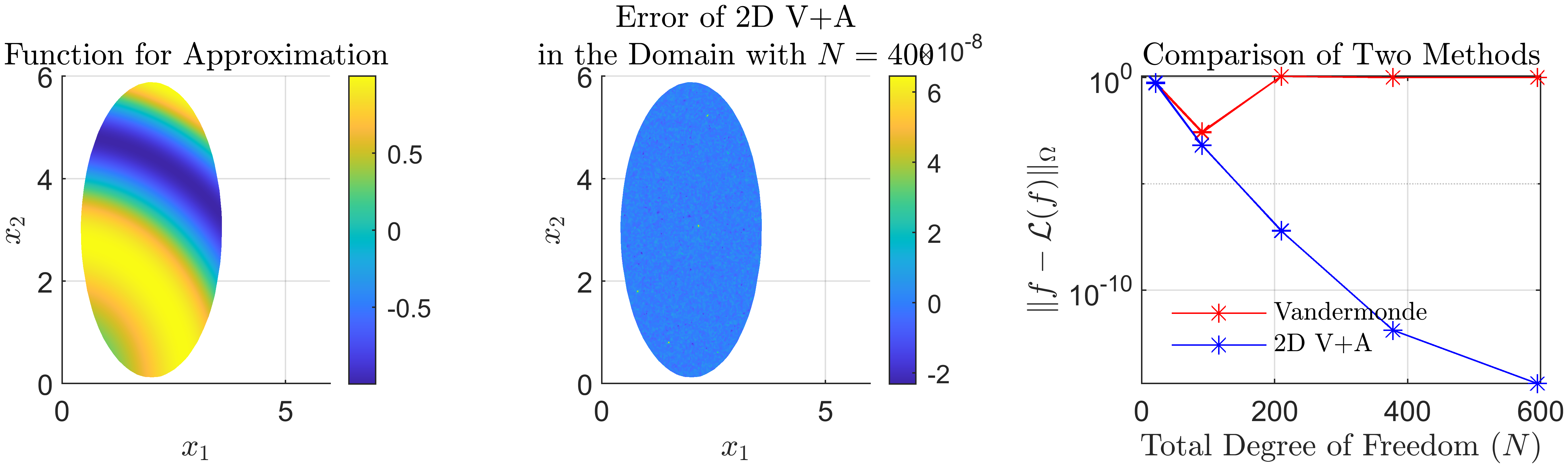
(V+A Polynomial Approximation on 2D Irregular Domain) We approximate the same function on an elliptical domain. We sample the points using the rejection sampling method. Namely, we enclose the domain in a hypercube domain and draw independent and identically distributed (i.i.d.) random samples from the uniform probability measure on . The acceptance rate for our domain is . We end the rejection sampler once we have a total of sample points55 5 More details on the sampling complexity are discussed in Section 4.2.2.. We plot the bivariate approximation result for the irregular domain in Figure 3. Again, the Vandermonde method fails for any , but the least squares approximation using the V+A method gives a stable error reduction to for . Since the Arnoldi orthogonalization generates a basis in the domain, the error for the least-squares approximation does not worsen when we switch from the tensor-product domain to the irregular domain. This example illustrates that the V+A algorithm can adapt to different discrete measures and non-tensor product domains.
Example 3.3.
(V+A Polynomial Approximation for 2D Non-Differential Functions) We test the least squares approximation with the V+A method on a non-differential function in the irregular domain. We found that the error reduction for the non-smooth function is much slower than the error reduction for the smooth function as illustrated in the right plot of Figure 4. The slow convergence in the error reduction is not caused by the least squares approximation using the V+A method; it is because polynomials are not great for approximating non-smooth functions. In other words, no polynomials in the space can converge rapidly to such non-differentiable functions. Additionally, the smoothness requirement of the function is stricter for higher dimensional domains. As we observe from the right plot of Figure 4, the 2D least-squares approximation of a non-smooth function exhibits a slower error reduction than the 1D least-squares approximation of a non-smooth function. The theoretical results for convergence and explanations of these phenomena are discussed in Section 4.3.2 and Theorem 4.7.
Example 3.4.
(Orthogonal Basis on vs. on ) We compare the least squares approximation using the V+A method with the least squares approximation using the orthogonal basis on the bounding domain (referred to as the ‘orthogonal basis on the bounding domain approximation’). In the orthogonal basis on the bounding domain approximation, we enclose the irregular domain in a hypercube domain, , and create an orthonormal basis for the bounding tensor-product domain using orthonormal Legendre polynomials66 6 This method is somewhat close to polynomial frame approximation [5], however it is not the same as we do not use regularization, e.g. truncated SVD, as here we aim to observe the effect of the V+A orthogonalization. More generally, we view an extensive comparison between frame approximation and V+A-based approximation a topic for future work.. We generate a numerical example using the function and the domain shown in Figure 3. In the numerical experiments, the 2D orthonormal Legendre polynomial basis is generated by sampling equispaced points on the tensor product domain and using orthogonalization techniques (such as QR or Gram-Schmidt process) to obtain the discrete orthogonal Legendre polynomials. An illustration of the sample points where the orthogonal polynomials are generated is given in Figure 5.
As given in the left plot of Figure 4, both methods provide a well-conditioned and accurate approximation. Using the same number of sample points , the orthogonal basis on the bounding domain approximation is slightly less accurate than the least squares approximation with the V+A method. This is partly because, in the orthogonal basis on the bounding domain approximation, the sample points are distributed across the entire tensor-product domain , with only about 59.59% of the sample points inside the domain . In contrast, in the least squares approximation with the V+A method, all sample points are within and contribute to the approximation.
Even if we increase the number of sample points for the orthogonal basis on the bounding domain approximation to to have approximately the same number of sample points within , the orthogonal basis on the bounding domain approximation with increased sample points remains slightly less accurate. This is because the Legendre polynomials are orthonormal for the tensor domain rather than for the elliptical domain. The orthonormal basis is no longer orthogonal when restricting the Legendre polynomials to an elliptical subdomain.


Example 3.5.
(V+A Polynomial Approximation for Higher Dimensional Multivariate Functions) Figure 6 presents preliminary numerical experiments on using V+A for high-dimensional function approximation (specifically, for ). In the cases of and , the least squares approximation using the V+A algorithm consistently reduces error for both tensor product and irregular domains, while the Vandermonde approximation is inaccurate due to ill-conditioning. These examples highlight the effectiveness of least-squares approximations using the V+A algorithm in higher-dimensional multivariate functions and non-tensor product domains. It is important to note that the multivariate V+A algorithm (Algorithm 3) and the theories we prove in this paper for multivariate V+A are applicable for . However, due to the growth of the polynomial basis with the dimensionality of functional approximation (i.e., for both polynomial spaces), the CPU time required for numerical experiments on higher-dimensional multivariate functions is affected by the curse of dimensionality. To overcome this, one may need to combine V+A with e.g. sparse grids [12]. The design of practical and scalable algorithms for high-dimensional functional approximation is a task we defer to future work.


4 Sample Complexity and Convergence of Multivariate V+A
In this section, we establish the sample complexity and convergence properties of the least squares approximation using the V+A algorithm for the total degree space. Note that the analysis follows naturally for the maximum degree of polynomial space, up to -dependent constants. We demonstrate that, across many domains, utilizing either equispaced points or random sample points, the V+A approximant with degrees of freedom is near-optimal. Namely, the error of the approximation is within a polynomial factor of that of the best approximation, for instance, where the notation involves constants that depend on . Furthermore, we prove that, when the sample complexity condition is satisfied, the error of the least squares approximation using the V+A algorithm converges at a spectral rate. Specifically,
| (11) |
where is the dimension of the variables (i.e., ), and is the highest order of the derivative of that exists and is continuous (i.e., smoothness).
The proofs and key contributions for this section are structured as follows.
- 1.
We first prove that convex bodies or finite unions of convex bodies satisfy the Markov property for total degree polynomial space (and also maximum degree space), such that
(Markov Condition) where is a domain-dependent constant. We highlight that this Markov property for the domain and the polynomial space is crucial for proving the sample complexity. Note that the constant for the Markov property (for total degree polynomial space and maximum degree space) differs by a factor depending on (Section 4.1).
- 2.
Under the Markov property condition, we can form a set of equispaced sample points, such that the maximum absolute value of the polynomial in is bounded by a constant multiplying the maximum absolute value of the polynomial at sample points , (Section 4.2). To the best of our knowledge, the Markov property and complexity results of this kind have only been established for total polynomial spaces in the literature [14, 25, 26, 38], but not specifically for maximum degree space.
- 3.
Then, we demonstrate V+A gives a near-optimal convergence rate (Section 4.3) for the total degree polynomial spaces77 7 In exact arithmetic, the V+A approximation is the same as that of a least-squares solution based on any basis, as long as the span of the bases is the same. The convergence results that therefore apply to any method based on least-squares, without the V+A orthogonalization. Of course, in finite precision, V+A can make a dramatic difference. For this reason, while the convergence results would hold for a least-squares method employing any basis, we often specify the use of V+A, as otherwise the theory may not be reflected in actual computations. .
- 4.
4.1 Markov Inequality
In this section, we demonstrate that (Markov Condition) holds for a variety of domains. We start with the simplest domain with . For univariate polynomial space, the two polynomial spaces overlap, Thus, the Markov condition for is given in [38].
Lemma 4.1.
(Markov Condition for ) For with , then
Lemma 4.2.
(Markov Condition for ) Let be a convex body, i.e., a convex compact set with a non-empty interior. Let and be a polynomial consisting of terms of at most with for . Then, the following results hold.
- 1.
Let such that . Assume also , then
Here is the minimal distance between two parallel supporting hyperplanes for and .
- 2.
For any multivariate polynomial with order and without the condition , a similar inequality holds true
Proof.
We start by proving the first result. We omit the trivial case when is constant. Under the assumption that , if is not a constant, this implies that , we must have on the boundary .
Let , and let be the hyperplane with normal which passes through . [38, Lemma 3.1] proved that is a supporting hyperplane of . Namely, and contains no interior points of . Now, assume is an outer normal for , and let be the supporting hyperplane with outer normal lying a distance from . Let . The line segment lies in by convexity, and
| , where , is a polynomial in with order . | (12) |
This polynomial is bounded by for . Since polynomials are translation invariant, Lemma 4.1 yields
where the last equality comes from . Also, since is the minimal distance between two parallel supporting hyperplanes for , we have . Therefore, By the definitions of -norm and , we deduce that . Extending the first result to the second result follows the same proof as in [38, Thm 3.1]. ∎
Remark 4.1.
Lemma 4.2 is adapted from [38, Lemma 3.1 & Thm 3.1]. In [38], the theorem was originally designed for the total degree polynomial space, and the bounds were given as:
for Results 1–2, respectively. When the polynomial space is the total degree space, , and Lemma 4.2 reduces to [38, Lemma 3.1 & Thm 3.1]. Our theorem also applies to the maximum degree where .
Theorem 4.1.
Let , and assume is a convex body. The multivariate polynomial with order satisfies the Markov condition in ,
| (Markov Condition) |
where for the maximum degree space, and for the total degree space. is the minimal distance between two parallel supporting hyperplanes for .
4.2 Sampling
We prove in this section that if equispaced sample points are chosen from a domain of a convex body or finite unions of convex bodies, then the maximum absolute value of the polynomial in is bounded by a constant multiplying the maximum absolute value of the polynomial at sample points , Since the constant for the Markov property only differs by a factor depending on (Theorem 4.1), the same order of sample complexity results apply to both the maximum degree and total degree spaces up to a -dependent constant. In a high-dimensional domain, it is sometimes easier to generate sample points randomly from the domain by rejection sampling. Therefore, in Section 4.2.2, we prove that with random sample points generated i.i.d. from a uniform measure, also holds with high probability for the maximum degree and total degree spaces up to a -dependent constant.
4.2.1 Deterministic Sample Points
We define equispaced discretization in Definition 4.1 and the sample complexity for equispaced sample points is given in Theorem 4.2.
Definition 4.1.
(Equispaced Discretization) Let be a compact domain and a bounding box containing . An equispaced discretization of is constructed by first defining an equispaced grid of points on , and subsequently restricting this grid to the points contained within . We write for the set of equispaced points in .
Theorem 4.2.
Let with be a convex body (i.e., a convex compact set with a non-empty interior) or finite unions of convex bodies. Let be a fixed constant. Construct a set of sample points such that for all , we have
| (Mesh Condition) |
where for the maximum degree space, and for the total degree space. Then,
| (13) |
for all multivariate polynomials. Using equispaced discretization as in Definition 4.1, the cardinality of satisfies , where is the number of basis functions. Note that the notation involves constants that depend on .
Proof.
The proof is similar to [14] (3.13)–(3.18). We have sharpened the upper bound for in (Mesh Condition) by a factor of . For any fixed (i.e., maximum degree, total degree), let such that the maximum value is attached at this point and for all we have such that . Then, using the mean value theorem, there exists on the line connecting to such that
| (14) |
where represents the line connecting to and .
Since is convex, we have . Theorem 4.1 gives that . Together with (Mesh Condition), we deduce that
where the last inequality comes from . Hence,
We deduce that . To prove the second argument regarding the cardinality of the mesh, we construct the mesh using a standard discretization process. For , we enclose in a -dimensional hypercube . We then cover with equispaced grids dense enough such that (Mesh Condition) is satisfied. This gives us number of nodes for the mesh. Lastly, the extension from a convex domain to a domain with the finite union of convex bodies is a direct application of [14, Lemma 4(i)]. ∎
Remark 4.2.
(Equispaced Sampling Method) Definition 4.1 and Theorem 4.2 provide us with a way to discretize the domain and choose sample points that can control the size of the discrete orthogonal polynomial. For , we enclose in a -dimensional hypercube . We then cover with equispaced grids dense enough such that (Mesh Condition) is satisfied which gives us number of nodes.
Note that the deterministic sampling method can be further improved in two ways. Firstly, instead of sampling in the hypercube domain , one could sample directly on using rejection sampling. Details on the randomized sampling method are discussed in Section 4.2.2. Secondly, instead of taking equispaced samples, we can choose a set of sample points with a ‘near-optimal weight’. Details on near-optimal sampling strategy are discussed in Section 5.
4.2.2 Randomized Sample Points
Theorem 8 gives the sample complexity for random sample points.
Theorem 4.3.
(Randomized Sampling Method) Let with be a convex body or finite union of convex bodies. Let be a set of points independently and uniformly sampled from . Let , and set . Then, with probability at least for the total degree polynomial spaces88 8 The same order of result is true for the maximum degree polynomial spaces, up to a -dependent constant..
Proof.
We prove this theorem using a similar approach to [39, Thm 4.1]. For the set of random sample points to satisfy (Mesh Condition), we need to prove that with high probability for every , one can find a point in such that their distance is at most . Specifically, for every , is satisfied with high probability where denotes the closed ball with center and radius . We have
The first equality follows from the i.i.d sampling nature of the random sample points. Note that denotes the cardinality of . The first inequality is given in the proof of [39, Thm 4.1]. By taking with , we achieve with probability at least . Applying Theorem 4.2 completes the proof. ∎
4.3 Convergence of Multivariate Vandermonde with Arnoldi
4.3.1 Error Bound
Theorem 4.4.
Let be a continuous multivariate function. Let with be a convex body or finite unions of convex bodies. Let be the best polynomial approximation of in the total degree polynomial space, such that for all . Construct a set of equispaced sample points as described in Remark 4.2, with . Applying Algorithm 3 using the sample points , the error of the least squares approximation satisfies99 9 The bound for the maximum degree space can be deduced similarly up to a -dependent constant.
| (15) |
where the columns of are the values of the discrete orthogonal basis generated by V+A at the sample points . The matrix -norm is defined as the largest absolute value of the matrix.
Proof.
Denote . We have
| (16) |
Since , we write it as a linear combination of discrete orthogonal polynomials where According to (6), where is a vector with entries as . Using Theorem 4.2, we have
| (17) |
Substituting (17) into (16) gives the first inequality in (15). Using the matrix property and the sample complexity assumption , we arrive at the second inequality in (15). ∎
Remark 4.3.
Example 4.5.
(Improved Numerical Error Bound on Certain Domains) Due to the special properties of the V+A basis (i.e., ), for the intervals, 2D tensor product domain, and other domains (as indicated in Figure 8), our numerical examples suggest that the least-squares approximant gives a tighter error bound than (15) in Theorem 4.4,
In other words, with equispaced sample points, scales like in the domains that we tested. For intervals and 2D tensor product domains the discrete orthogonal basis generated by equispaced sample points resembles the scaled Legendre polynomials, such that for and for The scaled Legendre polynomials for and are defined as follows.
Definition 4.2.
(Univariate Scaled Legendre Polynomials) For any interval with , we define the scaled univariate Legendre polynomials as
is the linear map from to and is the th standard univariate Legendre polynomials. The scaled Legendre polynomials are orthonormal in , such that for any .
Definition 4.3.
(Multivariate Scaled Legendre Polynomials) For tensor–product domain with for , we define the scaled multivariate Legendre polynomials as
with maps to . Note that is the standard multivariate Legendre polynomials
is the degree for the th entry . The scaled Legendre polynomials are orthonormal in , such that for any .
We give a brief justification for the tighter error bound than (15) in these cases. Firstly, we rewrite in expanded form
The discrete orthogonal polynomials generated equispaced points in real intervals are well approximated by the scaled Legendre polynomials. Therefore, is well approximated by the size maximum absolute value of the scaled Legendre polynomials . On the other hand, is small in the majority of the interval and only takes large values near the endpoints (Figure 7). The supremum of has a scaling of in an interval of length . The mean value of the absolute sum of the discrete orthogonal polynomials, , is relatively constant as grows. Our numerical experiment shows that when increases from to . As a result, together gives an upper bound for , that is, . Similar arguments follow for the 2D domains and the bound in 2D is obtained using


Remark 4.4.
(Relationship to Lebesgue Constant) The bound (15) in Theorem 4.4 is analogous to the bound in [36] involving the Lebesgue Constant ,
| (Lebesgue Constant Bound) |
where the Lebesgue constant is defined as the norm of the linear operator [36, 37],
where represents bounded and continuous functions. That said, the relationship between (15) and (Lebesgue Constant Bound) appears to be unknown in the literature. To compare these two bounds, we plot the constant which is in (15) against which is in (Lebesgue Constant Bound) in Figure 9. From the plot, we observe that these two bounds are of a similar order of magnitude same order of magnitude in the domains that we tested.

4.3.2 Convergence Rate
Following from Theorem 4.4, to understand how changes with the order of the index , we need to establish a bound for as increases. The bound is provided in Theorem 4.6, adapted from [8, Thm 1].
Theorem 4.6.
Let be a function of compact support on and be a compact subset of which contains the support of . Let where is the set of functions that have continuous derivatives up to total order . Then,
where is the best polynomial approximation in . is a positive constant depending only on and the diameter of .
Remark 4.5.
Using Theorem 4.4 and (15) in Theorem 4.2, we can deduce the rate of convergence of the least squares approximation generated by the V+A algorithm (Algorithm 3).
Theorem 4.7.
Let with be a convex body or finite unions of convex bodies. Let . Construct a set of equispaced sample points as described in Remark 4.2, with . Apply Algorithm 3 using the sample points , the error of the least squares approximation satisfies
| (19) |
where , is the order of the indices and is the total degree of freedom.
Remark 4.6.
Remark 4.7.
(Generalization to Domains with Markov Properties) As we can see in the proof of Theorem 4.2, the convexity of the domain is only used to deduce (Markov Condition) in Theorem 4.1. Therefore, Theorems 4.2, 8, 4.4 and 4.7 can be generalized to any domains satisfying (Markov Condition).
Example 4.8.
(Convergence Rate for Functions with Different Smoothness) We test the least squares approximation using the V+A algorithm for functions of specific smoothness in 1D and 2D. Note that the index set for the 2D example is the total degree index set. For smoothness and dimension , let
| (20) |
We also set . Clearly, for .
For fixed , , and , the term is the same for all functions. Thus, the improvement in convergence rates of the smoother functions comes from . Since for tensor-product domains, the least-squares approximations of and converge like and in 1D and and in 2D, respectively. The convergence rates of the four bivariate functions are approximately the square root of the convergence rates of the univariate counterparts. This is expected as we only have degrees of freedom in the or the directions for the bivariate approximation.

4.4 Related Work on Sample Complexity
In this subsection, we discuss the difference in construction between the sample complexity of the least squares approximation using the V+A Algorithm and the sample complexity of polynomial frame approximation.
There are many existing proofs for the sample complexity of polynomial approximations [4, 5, 15, 16, 30]. For instance, in [15, 16], the proof by Cohen et al. first constructs a -continuous orthogonal basis , such that Then, the solution of their least-squares problem can be computed by solving the Gram matrix system, where the th entries of is for and . The purpose of their analysis is to find how many sample points we need such that the discrete measure inherits the orthogonality of . Namely, how to choose such that
Using the exponentially decreasing bounds on tail distributions , Cohen et al. proved that random sample points is enough to obtain a stable least-squares approximation.
In [5], Adcock and Huybrechs give different proof for the sample complexity of frame approximation on irregular domains. The key step of the proof uses the Nikolskii inequality [29] on the bounding tensor-product domain
| (21) |
where is a constant that depends on the domain and the sample complexity. They proved that the least squares are near-optimal if the domain satisfies the -rectangle property. Namely, the bounding domain can be written as a (possibly overlapping and uncountable) union of hyperrectangles where is the value of . The sample complexity required scales by where is the total degree of freedom. Similar to the Markov constant introduced in (Markov Condition), the parameter in [5] is also independent of the bounding domain and is a constant that depends on .
Although sample complexity results obtained for the least squares approximation using the frame approximation and using the V+A method are similar, the idea and the construction of the proof are different. Firstly, in polynomial frame approximation, the proof starts with a continuous orthogonal polynomial and explores the distribution of sample points such that the discrete least-squares matrix is approximately orthogonal (i.e., ). By construction in V+A, we start with a discrete orthogonal basis (i.e., ) and examine the behaviours of these discrete orthogonal polynomials in the domain. Another difference is that these two approaches build the bound using different norm spaces in different domains. In V+A, we use the suprema of discrete orthogonal polynomials, , while in the polynomial frame approach, the Nikolskii inequality uses the norm, . The analysis for the least squares approximation using V+A method applies to the maximum degree or total degree polynomial spaces. In contrast, the analysis in [5] provides a more general result regarding polynomial spaces, extending to any polynomial space defined by a lower set. This includes maximum degree, total degree, and hyperbolic cross polynomial spaces. Current sample complexity analysis (derived via Lemma (4.2)) results in a scaling of for the hyperbolic cross index set. This scaling is less favorable compared to the scaling reported in [5], although the domain assumptions differ, and the error bound in that case is measured in the norm rather than the norm. Further investigation into improving the sample complexity analysis for hyperbolic cross polynomial spaces remains an open area of research. In terms of the domain, the analysis in [5] requires the bounding domain can be written as a (possibly overlapping and uncountable) union of hyperrectangles , whereas the analysis for the least squares approximation using V+A method holds for all domain satisfying (Markov Condition) (Remark 4.7).
More recently, Adcock and Shadrin [6] demonstrated that with linear oversampling of equispaced sample points and polynomial extensions over an extended interval, the equispaced samples become near-optimal for polynomial frame approximation in 1D. They propose a well-conditioned method that ensures exponential decay of the error, reaching a finite, user-controlled tolerance. In the following section, we will explore the use of the weighted least-squares algorithm and the multivariate V+A algorithm to give a well-conditioned and near-optimal polynomial approximation.
5 Near-Optimal Sampling Strategy for V+A
In this section, we propose a new variant of the weighted least-squares algorithm that uses the multivariate V+A to create the discrete orthogonal basis. We refer to our V+A weighted least-squares algorithm as VA+Weight.
In [2, 3, 16, 30], the authors gave comprehensive analyses on this weighted sampling strategy and proved that only sample points are needed for a well-conditioned and accurate approximation. A recent work [1] provides a comprehensive review on optimal sampling for (weighted) least-squares approximation in arbitrary linear spaces, introducing the Christoffel function as a key quantity in the analysis of (weighted) least-squares approximation from random samples. In VA+Weight, we use the same weighting measure as in [2]. But instead of creating the discrete orthogonal basis with QR factorization, we use V+A as the orthogonalization strategy for the Vandermonde basis. Since the Vandermonde matrix is usually highly ill-conditioned, and computing its factor incurs errors proportional to the condition number of [23, Ch. 19]. Even though the QR factorization is a stable orthogonalization technique, the discrete orthogonal basis generated from could still be inaccurate. We refer to the weighted least-squares approximation using the QR factorization as QR+Weight. Along with multiple numerical examples, we illustrate that VA+Weight gives more accurate approximations than QR+Weight for high-degree polynomial approximations. Due to the reduced sample density, VA+Weight also gives a lower online computational cost than the unweighted V+A least-squares method. Moreover, VA+Weight acts as a practical tool for selecting the near-optimal distribution of sample points in a high-dimensional irregular domain.
The section is arranged as follows. In Section 5.1, we explain the algorithm and the numerical setup for the weighted least-squares approximation. We provide proof of the stability of the weighting measure for sample points. In Section 5.2, we give numerical examples to compare the VA+Weight and QR+Weight algorithms.
5.1 Weighted Least-Squares Approximation
The VA+Weight algorithm is presented in Algorithm 5 and the remarks for the algorithm are given in Remark 5.1. Algorithm 5 is a V+A variant of Method 1 in [2].
with Vandermonde basis ;
Number of sample points and such that .
Output: The coefficients of the polynomial approximant.
Step 2: Construct Vandermonde matrix with the th entry as . If , go to Step 3, else go back to Step 1.
Step 3: Apply Algorithm 3 to to generate such that .
Step 4: Define a probability distribution on , such that for where is the Frobenius norm and are the th entry of .
Step 5: Draw integers independently from . Define and as the corresponding scaled rows of and , such that the point-wise entries are
Step 6: Solve the least-squares problem by the MATLAB backslash command. Approximate the value of using the evaluation algorithm in Algorithm 4 and give the output.
Remark 5.1.
Details for implementing Algorithm 5 are as follows.
- 1.
could be a convex body or finite unions of convex bodies or other domains that satisfy (Markov Condition) (See Remark 4.7)
- 2.
In our numerical implementation, unless otherwise stated, we choose and such that .
- 3.
We assume that it is possible to draw samples from the uniform measure in Step 1. We use the uniform rejection sampling method to draw samples. We end the rejection sampler once we have enough sample points.
- 4.
To ensure that in Step 2 of the algorithm, if is rank deficient, we add additional sample points until .
- 5.
The construction of uses Algorithm 3. Numerically, the orthogonalization algorithm is subject to a loss of orthogonality due to numerical cancellation. The numerically constructed discrete orthogonal basis is said to be -orthonormal for , namely, where . For any bounded domain , we define the infinity -norm of a bounded function as . In the multivariate V+A algorithm, we execute CGS twice for the orthogonalization, which gives a bound , where is the unit roundoff [23, Thm 19.4] and [19, Thm 2].
In Algorithm 5, for each sample point , represents the sum of the absolute value of discrete orthogonal polynomials at . The weighting measure can be interpreted as choosing the sample points that maximize the absolute sum of the discrete orthogonal polynomials at the sample points. Heuristically, this weighting measure makes sense as the supremum usually happens near the boundaries and corners of the domain. Many sampling measures, such as Chebyshev points in real intervals and Padua points [10, 13] in higher dimensional tensor-product domains have highlighted the importance of sample points near the boundary and corners.
is the number of points we selected from a total of sample points. The main question that we analyze in this section is how large needs to be chosen in relation to to ensure a near-optimal approximation. As we will prove later, with the probability distribution defined in Step 4, a log-linear scaling of is enough for a well-conditioned, near-optimal weighted least-squares approximation (provided that is large enough). The reduced sample complexity in Algorithm 5 gives a reduced online computational cost. The computational cost for Algorithm 5 is dominated by the cost of Step 3 and Step 6, which are flops and flops, respectively. Since we need random sample points to generate a randomized admissible mesh for convex domains or unions of convex domains in , Algorithm 5 gives an online computational cost of while the unweighted least-squares method described in Section 3 requires .
Algorithm 5 can be interpreted as a weighted least-squares system with V+A orthogonalization. Using the weight matrix the weighted least-squares problem can be written as
| (22) |
where and are the matrix and the vector formed with selected rows of and in the unweighted system. is the vector of coefficients for the weighted least-squares estimator such that . Note that is defined as before, namely the discrete orthogonal polynomials generated by sample points. The estimator is solved using normal equations, such that
| (23) |
is the reduced Gram matrix.
Since the weighted least-squares estimator is found by solving system (23) and by taking the inverse of the matrix , for stability and convergence we need to ensure that the Gram matrix is well-conditioned. Also, we investigate how much deviates from . In other words, we want to understand whether the discrete orthogonal basis at the selected sample points acts as a good approximation to the discrete orthogonal basis at the full sample points . The following theorem adapted from [30, Thm 3] establishes these links.
Theorem 5.1.
(Well-Conditioning of Reduced Gram Matrix) Let , consider finding a weighted least-squares approximation in the polynomial space using Algorithm 5. Let and generate the discrete orthogonal basis using Step 3 of Algorithm 5. The numerically constructed discrete orthogonal basis is -orthonormal for , such that . For , and , if the following conditions hold,
| i) | |||
| ii) |
then, the matrix satisfies where is the identity matrix.
We give a sketch of the proof for Theorem 5.1. We write as
The first probability term is bounded using condition , the equality and the -orthogonality. The second probability term is bounded using the Bernstein Inequality and condition which gives a tail bound for sums of random matrices. A full proof of Theorem 5.1 can be found in [30, Thm 3].
Theorem 5.1 not only ensures that is well-conditioned with high probability but also guarantees that the weighted least-squares problem (23) is stable with high probability. Under the conditions of Theorem 5.1, we have . Using that for all , it follows that
| (24) |
Thus, we arrive at the stability result Numerical examples the change of condition number of with respect to can be found in Figure 5.1. We illustrate, with a numerical example, the growth of the condition number of Gram Matrix (i.e., ) with respect to for different sampling densities . In Figure 11, we plot the condition number of formed by the weighted sampling method in Step 5 of Algorithm 5. For each line in Figure 11, we choose to be different functions of . As illustrated by the plot, we need a sampling density of to prevent from growing exponentially.

To ensure the convergence of Algorithm 5, in addition to conditions and in Theorem 5.1, we also require a sample density of random sample points. This result is expected as we do need random sample points to form discrete orthogonal polynomials that are well-bounded in the domain. There are a few papers that discuss the convergence for Algorithm 5, namely [2, Thm 3.1-3.5], [5, Thm 6.6] and [30, Thm 2].
5.2 Numerical Examples for Weighted V+A Algorithm
In this subsection, we compare the VA+Weight algorithm with the QR+Weight algorithm. The two algorithms use the same weights, but the QR+Weight algorithm uses the QR factorization of the ill-conditioned Vandermonde matrix to create the discrete orthogonal basis.
In Figure 12, we plot the numerical results of approximating a smooth function using VA+Weight and QR+Weight in a real interval. As shown in the left plot, both algorithms converge with number of weighted sample points. Before the ill-conditioning of builds in, the two algorithms performed similarly as expected. Note that the error from the two approximations will not be the same as we selected the weighted sample points in a non-deterministic fashion (i.e., following the probability measure ). However, when the condition number of grows beyond the inverse of the machine epsilon for , the QR+Weight approximation has an error stagnating at as illustrated in the left plot of Figure 12. Although the QR factorization and the weighted sampling method generate a well-conditioned (Figure 12), the columns of do not approximate the orthogonal basis in the domain (Figure 13). Thus, accuracy is lost for large .

On the other hand, as shown in the right plot of Figure 12, VA+Weight approximation gives a stable error reduction down to . The error reduction in VA+Weight also matches with the error reduction in the unweighted least-squares approximations. This is because the discrete orthogonal polynomials generated by V+A are unaffected by the ill-conditioning of . The value of the th discrete orthogonal polynomial overlaps with the value of the th scaled Legendre polynomial in the domain (Figure 13).

The same patterns of convergence are found while approximating bivariate functions. As plotted in Figure 14, VA+Weight gives an approximation with higher accuracy than QR+Weight in both domains. The difference in the two approximations is less in the 2D domain than in the 1D domain. This is because the multivariate Vandermonde matrix is, in general, less ill-conditioned in 2D domains than in 1D domains. That said, the conditioning of the multivariate Vandermonde matrix varies greatly with the shape of the domain. VA+Weight provides a stable and generalized method for multivariate approximations in irregular domains.


Finding the best distribution of sample points in a high-dimensional irregular domain is an open question in the literature. We highlight that the weighting method in Algorithm 5 is a practical tool for finding the near-optimal distribution of the sample points. We plot the sample points selected by VA+Weight for different domains in Figure 15. Notice that the selected points are clustered near corners and boundaries. This distribution pattern matches the pattern in Padua points in tensor-product domains. This behaviour occurs because the measure we use to select sample points assigns a higher probability to points where the discrete orthogonal polynomials have larger absolute values. Typically, these points cluster near the boundaries. A simple example is the set of Chebyshev polynomials or Legendre polynomials in the interval , where the polynomials exhibit larger absolute values at the endpoints.

Finally, we note that different weighting measures can be used to improve different aspects of the approximation algorithm. As illustrated in the left two plots of Figure 16, the VA+Weight algorithm gives a similar accuracy as the unweighted V+A least-squares approximation but with improved efficiency. That said, the approximants obtained from VA+Weight are only near-optimal, but not the best polynomial approximation. We propose combining the multivariate V+A with Lawson’s algorithm (VA+Lawson) to obtain the best multivariate polynomial approximation. VA+Lawson is based on an iterative re-weighted least-squares process and can be used to improve the approximation accuracy. Our numerical experiments showed that through the VA+Lawson algorithm, we improved the approximation error from to . Moreover, we found an equioscillating error curve in 2D, a characteristic of the best polynomial approximation [32, Thm. 24.1].

6 Conclusions and Future Works
In this paper, we analyzed the multivariate Vandermonde with the Arnoldi method to approximate -dimensional functions on irregular domains. The V+A technique resolves the ill-conditioning issue of the Vandermonde matrix and builds the discrete orthogonal polynomials with respect to the domain. Our main theoretical result is the convergence of the multivariate V+A least-squares approximation for a large class of domains. The sample complexity required for convergence is quadratic in the degree of freedom of the approximation space, up to a logarithmic factor polynomial approximations in total degree and maximum degree polynomial spaces. For hyperbolic cross polynomial spaces, [5] proved a sample complexity scaling of under the norm, the study of hyperbolic cross polynomial spaces under the norm remains a topic for our future research. Using a suitable weighting measure, we showed that the sample complexity can be further improved. The weighted V+A least-squares method requires only log-linear sample complexity .
Our preliminary numerical results validate that the least squares approximation using the V+A method provides well-conditioned and near-optimal approximations for multivariate functions on (irregular) domains with the dimension ranging from to . Additionally, the (weighted) least squares approximation using the V+A method performs competitively with state-of-the-art orthogonalization techniques and can serve as a practical tool for selecting near-optimal distributions of sample points in irregular domains. It is important to note that Algorithm 3 and the theories we prove in this paper for multivariate V+A are applicable for . However, due to the growth of the polynomial basis with the dimensionality of functional approximation (i.e., for total degree and maximum degree polynomial spaces), the CPU time required for computations for even higher dimensions will soon become infeasible due to the curse of dimensionality. The development of practical and scalable algorithms for high-dimensional functional approximation is also deferred to future work.
V+A has many applications beyond least-squares fitting. Our numerical experiments showed that the VA+Lawson algorithm improves the approximation accuracy and generates an equioscillating error curve. Yet, the convergence profile for VA+Lawson still seems to be unknown and could be an objective of future work. Another extension under consideration involves using multivariate V+A in vector- and matrix-valued rational approximations [17, Subsec. 2.4]. Generally speaking, in any application that involves matrix operations of Vandermonde matrix (or its related form), it seems likely that the V+A procedure could be an effective idea to apply.
Acknowledgments: We thank the referees for their valuable input, which has improved our work. We also appreciate the questions and comments from Ben Adcock, which led to our research on the convergence of V+A in different polynomial spaces and smoothness spaces.
References
- [1] Ben Adcock. Optimal sampling for least-squares approximation. arXiv preprint arXiv:2409.02342, 2024.
- [2] Ben Adcock and Juan M Cardenas. Near-optimal sampling strategies for multivariate function approximation on general domains. SIAM J. Maths. of Data Sci., 2(3):607–630, 2020.
- [3] Ben Adcock, Juan M Cardenas, Nick Dexter, and Sebastian Moraga. Towards optimal sampling for learning sparse approximations in high dimensions. In High-Dimensional Optimization and Probability: With a View Towards Data Science, pages 9–77. Springer, 2022.
- [4] Ben Adcock and Daan Huybrechs. Frames and numerical approximation. SIAM Rev., 61(3):443–473, 2019.
- [5] Ben Adcock and Daan Huybrechs. Approximating smooth, multivariate functions on irregular domains. In Forum Math. Pi, Sigma, volume 8. Cambridge University Press, 2020.
- [6] Ben Adcock and Alexei Shadrin. Fast and stable approximation of analytic functions from equispaced samples via polynomial frames. Constructive Approximation, 57(2):257–294, 2023.
- [7] Anthony P Austin, Mohan Krishnamoorthy, Sven Leyffer, Stephen Mrenna, Juliane Müller, and Holger Schulz. Practical algorithms for multivariate rational approximation. Comput. Phys. Comm., 261:107663, 2021.
- [8] Thomas Bagby, Len Bos, and Norman Levenberg. Multivariate simultaneous approximation. Constructive approximation, 18(4):569–577, 2002.
- [9] Bernhard Beckermann. The condition number of real Vandermonde, Krylov and positive definite Hankel matrices. Numer. Math., 85(4):553–577, 2000.
- [10] Len Bos, Marco Caliari, Stefano De Marchi, Marco Vianello, and Yuan Xu. Bivariate Lagrange interpolation at the Padua points: the generating curve approach. J. Approx Theory, 143(1):15–25, 2006.
- [11] Pablo D Brubeck, Yuji Nakatsukasa, and Lloyd N Trefethen. Vandermonde with Arnoldi. SIAM Review, 63(2):405–415, 2021.
- [12] Hans-Joachim Bungartz and Michael Griebel. Sparse grids. actanum, 13:147–269, 2004.
- [13] Marco Caliari, Stefano De Marchi, and Marco Vianello. Bivariate polynomial interpolation on the square at new nodal sets. J. Comput. Appl. Math., 165(2):261–274, 2005.
- [14] Jean-Paul Calvi and Norman Levenberg. Uniform approximation by discrete least squares polynomials. J. Approx. Theory, 152(1):82–100, 2008.
- [15] Albert Cohen, Mark A Davenport, and Dany Leviatan. On the stability and accuracy of least squares approximations. Found Comut Math, 13(5):819–834, 2013.
- [16] Albert Cohen and Giovanni Migliorati. Optimal weighted least-squares methods. SIAM J. Comp. Maths., 3:181–203, 2017.
- [17] Zlatko Drmac, Serkan Gugercin, and Christopher Beattie. Vector fitting for matrix-valued rational approximation. SIAM J. Sci. Comp., 37(5):A2346–A2379, 2015.
- [18] Walter Gautschi. Orthogonal polynomials: computation and approximation. OUP Oxford, 2004.
- [19] Luc Giraud, Julien Langou, Miroslav Rozlovzník, and Jasper van den Eshof. Rounding error analysis of the classical Gram-schmidt orthogonalization process. Numer. Math., 101(1):87–100, 2005.
- [20] Abinand Gopal and Lloyd N Trefethen. Solving Laplace problems with corner singularities via rational functions. SIAM J. Numer. Anal., 57(5):2074–2094, 2019.
- [21] WB Gragg and L Reichel. On the application of orthogonal polynomials to the iterative solution of linear systems of equations with indefinite or non-Hermitian matrices. Linear Algebra Appl, 88:349–371, 1987.
- [22] Björn Gustafsson, Mihai Putinar, Edward B Saff, and Nikos Stylianopoulos. Bergman polynomials on an archipelago: estimates, zeros and shape reconstruction. Adv. Math., 222(4):1405–1460, 2009.
- [23] Nicholas J Higham. Accuracy and stability of numerical algorithms. SIAM, 2002.
- [24] Jeffrey M Hokanson. Multivariate rational approximation using a stabilized Sanathanan-Koerner iteration. arXiv preprint arXiv:2009.10803, 2020.
- [25] Oliver Dimon Kellogg. On bounded polynomials in several variables. Mathematische Zeitschrift, 27(1):55–64, 1928.
- [26] András Kroó. On the approximation of convex bodies by convex algebraic level surfaces. Journal of Approximation Theory, 162(3):628–637, 2010.
- [27] Mykhailo Kuian, Lothar Reichel, and Sergij Shiyanovskii. Optimally conditioned Vandermonde-like matrices. SIAM J. Matrix Anal. Appl., 40(4):1399–1424, 2019.
- [28] Charles Lawrence Lawson. Contribution to the theory of linear least maximum approximation. Ph. D. dissertation, Univ. Calif., 1961.
- [29] Giovanni Migliorati. Multivariate Markov-type and Nikolskii-type inequalities for polynomials associated with downward closed multi-index sets. J. Approx. Theory, 189:137–159, 2015.
- [30] Giovanni Migliorati. Multivariate approximation of functions on irregular domains by weighted least-squares methods. IMA J. Numer. Anal., 41(2):1293–1317, 2021.
- [31] Victor Y Pan. How bad are Vandermonde matrices? SIAM J. Matrix Anal. Appl., 37(2):676–694, 2016.
- [32] Michael James David Powell et al. Approximation theory and methods. Cambridge university press, 1981.
- [33] Herbert Stahl. Best uniform rational approximation of on . Bull New Ser Am Math Soc, 28(1):116–122, 1993.
- [34] Gabor Szeg. Orthogonal polynomials. Am Math Soc., 23, 1939.
- [35] Lloyd N Trefethen, J Andre C Weideman, and Thomas Schmelzer. Talbot quadratures and rational approximations. BIT Numer. Math., 46(3):653–670, 2006.
- [36] Marc Van Barel and Matthias Humet. Good point sets and corresponding weights for bivariate discrete least squares approximation. Dolomites Res. Notes Approx., 8(Special_Issue), 2015.
- [37] Marc Van Barel, Matthias Humet, and Laurent Sorber. Approximating optimal point configurations for multivariate polynomial interpolation. Electron. Trans. Numer. Anal., 42:41–63, 2014.
- [38] Don R Wilhelmsen. A Markov inequality in several dimensions. J. Approx. Theory, 11(3):216–220, 1974.
- [39] Yiming Xu and Akil Narayan. Randomized weakly admissible meshes. J. Approx. Theory, page 105835, 2022.
- [40] Yuan Xu. On discrete orthogonal polynomials of several variables. Advances in Applied Mathematics, 33(3):615–632, 2004.