跳到论文正文
W Papers独立论文阅读器 arXiv:2301.11808 论文正文 计算阅读时间 · 0%
引用这篇论文根据当前论文元数据生成,正式投稿前建议核对。


License: arXiv.org perpetual non-exclusive license
arXiv:2301.11808v2 [math.ST] 30 Oct 2023

Minimax Optimal Rate for Parameter Estimation in Multivariate Deviated Models

Dat Do* Affiliation: Department of Statistics Affiliation: University of Michigan at Ann Arbor Affiliation: Ann Arbor, MI 48109 Email: dodat@umich.edu    Huy Nguyen* Affiliation: Department of Statistics and Data Sciences Affiliation: The University of Texas at Austin Affiliation: Austin, TX 78712 Email: huynm@utexas.edu    Khai Nguyen Affiliation: Department of Statistics and Data Sciences Affiliation: The University of Texas at Austin Affiliation: Austin, TX 78712 Email: khainb@utexas.edu    Nhat Ho Affiliation: Department of Statistics and Data Sciences Affiliation: The University of Texas at Austin Affiliation: Austin, TX 78712 Email: minhnhat@utexas.edu
Abstract

We study the maximum likelihood estimation (MLE) in the multivariate deviated model where the data are generated from the density function (1−λ∗)​h0​(x)+λ∗​f​(x|μ∗,Σ∗)(1-\lambda^{\ast})h_{0}(x)+\lambda^{\ast}f(x|\mu^{\ast},\Sigma^{\ast}) in which h0h_{0} is a known function, λ∗∈[0,1]\lambda^{\ast}\in[0,1] and (μ∗,Σ∗)(\mu^{\ast},\Sigma^{\ast}) are unknown parameters to estimate. The main challenges in deriving the convergence rate of the MLE mainly come from two issues: (1) The interaction between the function h0h_{0} and the density function ff; (2) The deviated proportion λ∗\lambda^{\ast} can go to the extreme points of [0,1][0,1] as the sample size tends to infinity. To address these challenges, we develop the distinguishability condition to capture the linear independent relation between the function h0h_{0} and the density function ff. We then provide comprehensive convergence rates of the MLE via the vanishing rate of λ∗\lambda^{\ast} to zero as well as the distinguishability of two functions h0h_{0} and ff.

††footnotetext: ∗ Equal contribution.

1 Introduction

The goodness-of-fit test [11] is one of the foundational tools in statistics with several applications in data-driven scientific fields, namely kernel Stein discrepancy [27, 31], point processes [37] and Bayesian statistics [32], etc. Given a sample set of data and a pre-specified distribution with density function h0h_{0}, the test indicates whether the samples are reasonably distributed according to h0h_{0} (null hypothesis) or to another family of distributions {p(⋅|θ):θ∈Θ}\{p(\cdot|\theta):\theta\in\Theta\} (alternative hypothesis). It is worth noting that knowledge about the null hypothesis distribution can come from prior knowledge of scientists. A key to understanding the statistical efficiency of testing is via the likelihood ratio and the maximum likelihood estimation (MLE) methods. [6].

While traditional testing problems often assume the null distribution h0=p(⋅|θ0)h_{0}=p(\cdot|\theta_{0}) and the alternative one p(⋅|θ)p(\cdot|\theta) are from a single simple family of distributions such as exponential families, there are also many problems in science require to test h0h_{0} against the alternative f(⋅|θ)f(\cdot|\theta) that can be deviated from h0h_{0} by a distribution from a potentially different family. Specifically, in this paper, we consider the family of distributions named multivariate deviated model with density functions defined as follows:

pG​(x):=(1−λ)​h0​(x)+λ​f​(x|μ,Σ),\displaystyle p_{G}(x):=(1-\lambda)h_{0}(x)+\lambda f(x|\mu,\Sigma), (1)

where x∈ℝdx\in\mathbb{R}^{d}, G:=(λ,μ,Σ)G:=(\lambda,\mu,\Sigma) are the model’s parameters with λ∈[0,1]\lambda\in[0,1] being the deviated proportion (from h0h_{0}) and (μ,Σ)∈Θ×Ω(\mu,\Sigma)\in\Theta\times\Omega are parameters of a vector-matrix family of distributions ff, where Θ⊂ℝd\Theta\subset\mathbb{R}^{d} and Ω⊂ℝd×d\Omega\subset\mathbb{R}^{d\times d} being compact. When λ=0\lambda=0, this recovers the null hypothesis distribution h0h_{0}.

The deviated model can be motivated by many applications in science. For instance, in microarray data analysis, it can be used to detect differentially expressed genes under two or more conditions [1, 2], where h0h_{0} is the uniform distribution and f(⋅|μ,Σ)f(\cdot|\mu,\Sigma) is required to estimate. Many other applications can be seen in many contamination problems in astronomy and biology [29]. Besides, the deviated model can also be viewed as a low-rank adaptation model in the domain adaptation problem [23], where h0h_{0} is a pre-trained model on large data, and ff is a simpler component to be estimated from the smaller data domain. Our goal in this paper is to study the parameter estimation rate of the deviated model.

Problem setup. Suppose that we observe nn i.i.d. samples X1,…,XnX_{1},\dots,X_{n} from the true multivariate deviated model:

pG∗​(x):=(1−λ∗)​h0​(x)+λ∗​f​(x|μ∗,Σ∗),\displaystyle p_{G_{*}}(x):=(1-\lambda^{*})h_{0}(x)+\lambda^{*}f(x|\mu^{*},\Sigma^{*}), (2)

where G∗:=(λ∗,μ∗,Σ∗)G_{*}:=(\lambda^{*},\mu^{*},\Sigma^{*}) are true but unknown parameters with λ∗≠0\lambda^{*}\neq 0. Throughout the paper, we allow G∗G_{*} to change with the sample size nn (see Appendix F.1 for a discussion). To facilitate our presentation, we suppress the dependence of G∗G_{*} on nn, and then estimate G∗G_{*} from the data. The main focus of this paper is to establish both a uniform convergence rate and minimax rate for parameter estimation via the MLE approach, which is given by:

G^n∈arg​maxG∈Ξ∑i=1nlogpG(Xi),\displaystyle\widehat{G}_{n}\in\argmax_{G\in\Xi}\sum_{i=1}^{n}\log p_{G}(X_{i}), (3)

where G^n:=(λ^n,μ^n,Σ^n)\widehat{G}_{n}:=(\widehat{\lambda}_{n},\widehat{\mu}_{n},\widehat{\Sigma}_{n}) and Ξ:=[0,1]×Θ×Ω\Xi:=[0,1]\times\Theta\times\Omega.

Contribution. There are two main challenges in studying the convergence rate of the MLE G^n\widehat{G}_{n}: (1) The interaction between the function h0h_{0} and the density function ff, e.g., h0h_{0} belongs to the family of ff and (μ∗,Σ∗)(\mu^{*},\Sigma^{*}) approaches h0h_{0} as the sample size nn goes to infinity; (2) The deviated proportion λ∗\lambda^{*} can go to the extreme points of [0,1][0,1] as the sample size goes to infinity and make the estimation become more challenging, because when λ∗=0\lambda^{*}=0, all the parameters (μ∗,Σ∗)(\mu^{*},\Sigma^{*}) yield the same model. To address these singularity and identifiability issues, we first develop the distinguishability condition to capture the linear independent relation between the function h0h_{0} and the density function ff. We then study the optimal convergence rate of parameters under both distinguishable and non-distinguishable settings of the multivariate deviated model. Our theoretical results can be summarized as follows:

1. Distinguishable settings: We demonstrate that as long as the function h0h_{0} and the density function ff are distinguishable, the convergence rate of λ^n\widehat{\lambda}_{n} to λ∗\lambda^{*} is 𝒪(n−1/2)\mathcal{O}(n^{-1/2}) while (μ^n,Σ^n)(\widehat{\mu}_{n},\widehat{\Sigma}_{n}) converges to (μ∗,Σ∗)(\mu^{*},\Sigma^{*}) at a rate determined by the vanishing rate of λ∗\lambda^{*} as follows:

λ∗∥(μ^n,Σ^n)−(μ∗,Σ∗)∥=𝒪(n−1/2).\displaystyle\lambda^{*}\|(\widehat{\mu}_{n},\widehat{\Sigma}_{n})-(\mu^{*},\Sigma^{*})\|=\mathcal{O}(n^{-1/2}).

It indicates that if λ∗\lambda^{*} goes to 0, the convergence rate of estimating (μ∗,Σ∗)(\mu^{*},\Sigma^{*}) is slower than the parametric rate.

2. Non-distinguishable settings: When h0h_{0} and ff are not distinguishable, it becomes complicated to capture the convergence rate of the MLE. To shed light on the behaviors of the MLE under the non-distinguishable settings of multivariate deviated model, we specifically study the settings when h0h_{0} belongs to the same family as ff, namely, h0(.)=f(.|μ0,Σ0)h_{0}(.)=f(.|\mu_{0},\Sigma_{0}) for some (μ0,Σ0)(\mu_{0},\Sigma_{0}). To precisely characterize the rates of the MLE under this setting, we consider the second-order strong identifiability of ff, which requires the linear independence up to second-order derivatives of ff with respect to its parameters. The second-order identifiability had also been considered in the literature to investigate the convergence rate of parameter estimation in finite mixtures [9, 28, 22, 21, 20, 19].

2.1. Strongly identifiable and non-distinguishable settings: When ff is strongly identifiable in the second order, we demonstrate that ∥(Δμ∗,ΔΣ∗)∥2|λ^n−λ∗|=𝒪(n−1/2)\|(\Delta\mu^{*},\Delta\Sigma^{*})\|^{2}|\widehat{\lambda}_{n}-\lambda^{*}|=\mathcal{O}(n^{-1/2}) and

λ∗(∥(Δμ∗,ΔΣ∗)∥+∥(Δμ^n,ΔΣ^n∥)∥(μ^n,Σ^n)−(μ∗,Σ∗)∥=𝒪(n−1/2),\displaystyle\lambda^{*}(\|(\Delta\mu^{*},\Delta\Sigma^{*})\|+\|(\Delta\widehat{\mu}_{n},\Delta\widehat{\Sigma}_{n}\|)\|(\widehat{\mu}_{n},\widehat{\Sigma}_{n})-(\mu^{*},\Sigma^{*})\|=\mathcal{O}(n^{-1/2}),

where Δ​μ:=μ−μ0\Delta\mu:=\mu-\mu_{0} and Δ​Σ:=Σ−Σ0\Delta\Sigma:=\Sigma-\Sigma_{0}. It indicates that the convergence rate of λ^n\widehat{\lambda}_{n} to λ∗\lambda^{*} depends on that of (μ∗,Σ∗)(\mu^{*},\Sigma^{*}) to (μ0,Σ0)(\mu_{0},\Sigma_{0}) while the convergence rate of (μ^n,Σ^n)(\widehat{\mu}_{n},\widehat{\Sigma}_{n}) to (μ∗,Σ∗)(\mu^{*},\Sigma^{*}) depends on both the rate of λ∗\lambda^{*} to 0 and the rate of (μ∗,Σ∗)(\mu^{*},\Sigma^{*}) to (μ0,Σ0)(\mu_{0},\Sigma_{0}). These results are strictly different from those in the distinguishable settings, which is mainly due to the non-distinguishability between h0h_{0} and ff.

2.2. Weakly identifiable and non-distinguishable settings: When ff is weakly identifiable, i.e., it is not strongly identifiable in the second order, we specifically consider the popular setting when ff is the density of a multivariate Gaussian distribution. The loss of the strong identifiability of the Gaussian distribution is due to the following partial differential equation (PDE) between the location and scale parameters (the heat equation):

∂2f∂μ​∂μ⊤​(x|μ,Σ)=2​∂f∂Σ​(x|μ,Σ).\displaystyle\dfrac{\partial^{2}{f}}{\partial{\mu}\partial\mu^{\top}}(x|\mu,\Sigma)=2\dfrac{\partial{f}}{\partial{\Sigma}}(x|\mu,\Sigma).

Due to the above PDE, the convergence rate of the MLE under this setting exhibits very different behaviors from those under the strongly identifiable setting. In particular, we prove that [∥Δμ∗∥4+∥ΔΣ∗∥2]|λ^n−λ∗|=𝒪(n−1/2)\left[\|\Delta\mu^{*}\|^{4}+\|\Delta\Sigma^{*}\|^{2}\right]|\widehat{\lambda}_{n}-\lambda^{*}|=\mathcal{O}(n^{-1/2}) and

λ∗(∥Δμ∗∥2+∥Δμ^n∥2+∥ΔΣ∗∥+∥ΔΣ^n∥)(∥μ^n−μ∗∥2+∥Σ^n−Σ∗∥)=𝒪(n−1/2).\displaystyle\lambda^{*}(\|\Delta\mu^{*}\|^{2}+\|\Delta\widehat{\mu}_{n}\|^{2}+\|\Delta\Sigma^{*}\|+\|\Delta\widehat{\Sigma}_{n}\|)(\|\widehat{\mu}_{n}-\mu^{*}\|^{2}+\|\widehat{\Sigma}_{n}-\Sigma^{*}\|)=\mathcal{O}(n^{-1/2}).

Notably, there is a mismatch in the orders of convergence rates of the location vector and covariance matrix. Furthermore, the rate of the deviated mixing proportion also depends on different orders of μ∗\mu^{*} to μ0\mu_{0} and Σ∗\Sigma^{*} to Σ0\Sigma_{0}. Such rich behaviors of the MLE are mainly due to the PDE between the location and scale parameters.

Comparing to moment methods. We would like to remark that the results for the MLE under the non-distinguishable settings in the paper are (much) tighter than those obtained from moment methods for a general mixture of two components in the literature. In particular, when ff is multivariate Gaussian distribution with fixed covariance matrix, i.e., ff is strongly identifiable in the second order and we do not estimate Σ∗\Sigma^{*}, an application of the results with moment methods from [36] to the deviated models leads to ∥Δμ∗∥3|λnmoment−λ∗|=𝒪(n−1/2)\|\Delta\mu^{*}\|^{3}|\lambda_{n}^{\text{moment}}-\lambda^{*}|=\mathcal{O}(n^{-1/2}) and λ∗∥μnmoment−μ∗∥3=𝒪(n−1/2)\lambda^{*}\|\mu_{n}^{\text{moment}}-\mu^{*}\|^{3}=\mathcal{O}(n^{-1/2}), which are much slower compared to the results for the MLE in the strongly identifiable and non-distinguishable settings, where (λnmoment,μnmoment)(\lambda_{n}^{\text{moment}},\mu_{n}^{\text{moment}}) denote moment estimators of λ∗\lambda^{*} and μ∗\mu^{*}.

When ff is a multivariate Gaussian density and we estimate both the location vector and covariance matrix, i.e., ff is weakly identifiable, an adaptation of the moment estimators from the seminal work [18] to the multivariate deviated models shows that λ∗∥∥μ~nmoment−μ∗∥6=𝒪(n−1/2)\lambda^{*}\|\|\tilde{\mu}_{n}^{\text{moment}}-\mu^{*}\|^{6}=\mathcal{O}(n^{-1/2}), λ∗∥∥Σ~nmoment−Σ∗∥3=𝒪(n−1/2)\lambda^{*}\|\|\tilde{\Sigma}_{n}^{\text{moment}}-\Sigma^{*}\|^{3}=\mathcal{O}(n^{-1/2}) and (∥Δμ∗∥6+∥ΔΣ∗∥3)|λ~nmoment−λ∗|=𝒪(n−1/2)(\|\Delta\mu^{*}\|^{6}+\|\Delta\Sigma^{*}\|^{3})|\tilde{\lambda}_{n}^{\text{moment}}-\lambda^{*}|=\mathcal{O}(n^{-1/2}), where (λ~nmoment,μ~nmoment,Σ~nmoment)(\tilde{\lambda}_{n}^{\text{moment}},\tilde{\mu}_{n}^{\text{moment}},\tilde{\Sigma}_{n}^{\text{moment}}) are moment estimators of (λ∗,μ∗,Σ∗)(\lambda^{*},\mu^{*},\Sigma^{*}). These results are also much slower than those of the MLE in weakly identifiable settings.

Other related work. The hypothesis testing and MLE problem related to the multivariate deviated model had been considered in previous work, including the problem of detecting sparse homogeneous and heteroscedastic mixtures [14, 15, 4, 3, 5, 34], the problem of determining the number of components [8, 26, 10, 24, 25], and the problem of multiple testing  [30, 12]. In particular, [4] considers testing problem for the deviated model with h0=N⁡(0,1)h_{0}=N(0,1) and f=N⁡(μ∗,1)f=N(\mu^{*},1) being one-dimensional Gaussian distributions. They show that no test can reliably detect λ∗=0\lambda^{*}=0 against λ∗>0\lambda^{*}>0 if λ∗μ∗=o(n−1/2)\lambda^{*}\mu^{*}=o(n^{-1/2}), while the Likelihood Ratio test can consistently do it when λ∗μ∗≳n−1/2+ϵ\lambda^{*}\mu^{*}\gtrsim n^{-1/2+\epsilon} for any ϵ>0\epsilon>0. However, no guarantee for estimation of λ∗\lambda^{*} and μ∗\mu^{*} is provided. In the same setting where ff is the density of a location Gaussian distribution, the convergence rate of parameter estimation in the deviated model had been studied in the work of [16]. Since the location Gaussian distribution is a special case of the strongly identifiable distribution, our result in the strongly identifiable and non-distinguishable settings is a generalization of the results in [16], but with a different proof technique as their proof technique relies strictly on the properties of the location Gaussian distribution.

Organization. The paper is organized as follows. In Section 2, we provide background on the identifiability and density estimation rate of the multivariate deviated model. Then, we establish the lower bounds of the Total Variation distance between two densities in terms of loss functions among parameters under both the distinguishable and non-distinguishable settings in Section 3. Next, we characterize the convergence rates of parameter estimation as well as derive the corresponding minimax lower bounds in Section 4. In Section 5, we carry out a simulation study to empirically verify our theoretical results before concluding the paper in Section 6. Rigorous proofs and additional results are deferred to the supplementary material.

Notations. For any a,b∈ℝa,b\in\mathbb{R}, we denote a∨b:=max⁡{a,b}a\vee b:=\max\left\{a,b\right\} and a∧b:=min⁡{a,b}a\wedge b:=\min\left\{a,b\right\}. Next, we say that h0h_{0} is identical to ff if h0​(x)=f⁡(x|μ0,Σ0)h_{0}(x)=f(x|\mu_{0},\Sigma_{0}) for some (μ0,Σ0)∈Θ×Σ(\mu_{0},\Sigma_{0})\in\Theta\times\Sigma. For each parameter G∈ΞG\in\Xi, let 𝔼pG\mathbb{E}_{p_{G}} be the expectation taken with respect to product measure with density pGp_{G}. Lastly, for any two density functions pp and qq (with respect to the Lebesgue measure mm), the Total Variation distance between them is given by V⁡(p,q):=12​∫|p⁡(x)−q⁡(x)|​𝑑m​(x)V(p,q):=\frac{1}{2}\int|p(x)-q(x)|dm(x), while we define their squared Hellinger distance as h2​(p,q):=12​∫[p⁡(x)−q⁡(x)]2​𝑑m​(x)h^{2}(p,q):=\frac{1}{2}\int[\sqrt{p(x)}-\sqrt{q(x)}]^{2}dm(x).

2 Preliminaries

2.1 Identifiability Condition

Our principal goal in this paper is to assess the statistical efficiency of parameter estimation from the MLE method. To do that, we should be able to guarantee the parameter identifiability of the deviated model (2), i.e., if pG​(x)=pG∗​(x)p_{G}(x)=p_{G_{*}}(x) for almost surely x∈𝒳x\in\mathcal{X} where G=(λ,μ,Σ)G=(\lambda,\mu,\Sigma), then G≡G∗G\equiv G_{*}. That identifiability condition leads to the following notion of distinguishability between the density function h0​(⋅)h_{0}(\cdot) and the family of density functions {f(⋅|μ,Σ):(μ,Σ)∈Θ×Ω}\{f(\cdot|\mu,\Sigma):(\mu,\Sigma)\in\Theta\times\Omega\}.

Definition 2.1 (Distinguishability).

We say that the family of density functions {f(⋅|μ,Σ),(μ,Σ)∈Θ×Ω}\{f(\cdot|\mu,\Sigma),(\mu,\Sigma)\in\Theta\times\Omega\} (or in short, ff) is distinguishable from h0h_{0} if the following holds:

  • A1.

    For any two distinct components (μ1,Σ1)(\mu_{1},\Sigma_{1}) and (μ2,Σ2)(\mu_{2},\Sigma_{2}), if we have real coefficients ηi\eta_{i} for 1≤i≤31\leq i\leq 3 such that η1​η2≤0\eta_{1}\eta_{2}\leq 0 and η1​f​(x|μ1,Σ1)+η2​f​(x|μ2,Σ2)+η3​h0​(x)=0\eta_{1}f(x|\mu_{1},\Sigma_{1})+\eta_{2}f(x|\mu_{2},\Sigma_{2})+\eta_{3}h_{0}(x)=0, for almost surely x∈ℝdx\in\mathbb{R}^{d}, then η1=η2=η3=0\eta_{1}=\eta_{2}=\eta_{3}=0.

We can verify that as long as ff is distinguishable from h0h_{0}, the parameter identifiability of our multivariate deviated model follows. In particular, assume that there exists G=(λ,μ,Σ)G=(\lambda,\mu,\Sigma) such that

(1−λ∗)​h0​(x)+λ∗​f​(x|μ∗,Σ∗)=(1−λ)​h0​(x)+λ​f​(x|μ,Σ),\displaystyle(1-\lambda^{*})h_{0}(x)+\lambda^{*}f(x|\mu^{*},\Sigma^{*})=(1-\lambda)h_{0}(x)+\lambda f(x|\mu,\Sigma), (4)

for almost surely x∈𝒳x\in\mathcal{X}. The above equation is equivalent to (λ−λ∗)​h0​(x)+λ∗​f​(x|μ∗,Σ∗)−λ​f​(x|μ,Σ)=0(\lambda-\lambda^{*})h_{0}(x)+\lambda^{*}f(x|\mu^{*},\Sigma^{*})-\lambda f(x|\mu,\Sigma)=0. Assume that ff is distinguishable from h0h_{0}, then equation (4) indicates that if (μ,Σ)≠(μ∗,Σ∗)(\mu,\Sigma)\neq(\mu^{*},\Sigma^{*}), we have λ=λ∗=0\lambda=\lambda^{*}=0. Since λ∗≠0\lambda^{*}\neq 0 from our assumption, we obtain that (μ,Σ)=(μ∗,Σ∗)(\mu,\Sigma)=(\mu^{*},\Sigma^{*}). As a result, equation (4) becomes (λ−λ∗)​h0​(x)+(λ∗−λ)​f​(x|μ,Σ)=0(\lambda-\lambda^{*})h_{0}(x)+(\lambda^{*}-\lambda)f(x|\mu,\Sigma)=0. By applying the distinguishability condition again, we get λ=λ∗\lambda=\lambda^{*}. Therefore, the multivariate deviated model (2) is identifiable.

In the following example, we will verify the distinguishability condition in Definition 2.1 given some specific choices of function h0h_{0} and density ff.

Example 2.2.

(a) Assume that ff belongs to a location family of density functions, i.e., f⁡(x|μ,Σ)=fΣ​(x−μ)f(x|\mu,\Sigma)=f_{\Sigma}(x-\mu) for all xx where Σ\Sigma is a fixed covariance matrix. If h0​(x)≠f​(x)h_{0}(x)\neq f(x) for almost surely x∈𝒳x\in\mathcal{X}, then ff is distinguishable from h0h_{0}.
(b) When h0h_{0} is a finite mixture of multivariate Gaussian densities and ff belongs to a class of multivariate Student’s density functions with any fixed odd degree of freedom ν>1\nu>1, we get that ff is distinguishable from h0h_{0}.
(c) When ff is identical to h0h_{0}, then ff is not distinguishable from h0h_{0}.

2.2 Convergence Rate of Density Estimation

Our strategy to obtain the convergence rate of the MLE G^n\widehat{G}_{n} is by first establishing the convergence rate of density pG^np_{\widehat{G}_{n}} and then studying the geometric inequalities between the parameter space and density space. For the former, the standard method is to use the empirical process theory [17, 33], while for the latter step, we investigate those inequalities under various settings of distinguishability in Section 3. Due to space constraints and the popularity of empirical process theory, we choose to informally present a main result for yielding the parametric convergence rate for density estimation in this section. For full explanation and definition, readers are referred to Appendix B. The convergence rate for density estimation can be characterized by bounding the complexity of the parameter space Ξ\Xi via a function called bracketing entropy integral 𝒥B​(ϵ,𝒫¯1/2​(Ξ,ϵ))\mathcal{J}_{B}(\epsilon,\overline{\mathcal{P}}^{1/2}(\Xi,\epsilon)) (cf. equation (8)).

Theorem 2.3.

Assume the following assumption holds:

  1. A2.

    Given a universal constant J>0J>0, there exists N>0N>0, possibly depending on Ξ\Xi, such that for all n≥Nn\geq N and all ϵ>(log⁡(n)/n)1/2\epsilon>(\log(n)/n)^{1/2}, we have 𝒥B​(ϵ,𝒫¯1/2​(Ξ,ϵ))≤J​n​ϵ2.\mathcal{J}_{B}(\epsilon,\overline{\mathcal{P}}^{1/2}(\Xi,\epsilon))\leq J\sqrt{n}\epsilon^{2}.

Then, there exists a constant C>0C>0 depending only on Ξ\Xi such that for all n≥1n\geq 1,

supG∗∈Ξ𝔼pG∗​h​(pG^n,pG∗)≤C​log⁡n/n.\sup_{G_{*}\in\Xi}\mathbb{E}_{p_{G_{*}}}h(p_{\widehat{G}_{n}},p_{G_{*}})\leq C\sqrt{\log n/n}.

Therefore, in order to get the convergence rate for density estimators based on the MLE method, we only need to check Assumption A2, which holds true for several parametric models [33]. For our model, we give an example that it holds for a general class of ff and h0h_{0}.

Proposition 2.4.

Suppose that both Θ\Theta and Ω\Omega are compact, and {f(x|μ,Σ):μ∈Θ,Σ∈Ω}\{f(x|\mu,\Sigma):\mu\in\Theta,\Sigma\in\Omega\} is a vector-matrix family of densities being uniformly bounded, Lipschitz, and light tail, i.e. there exists constants M,L,B,b1,b2,b3>0M,L,B,b_{1},b_{2},b_{3}>0 such that |f⁡(x|μ,Σ)|≤M,|f⁡(x|μ,Σ)−f⁡(x|μ′,Σ′)|≤L⁡(‖μ−μ′‖+‖Σ−Σ′‖)|f(x|\mu,\Sigma)|\leq M,|f(x|\mu,\Sigma)-f(x|\mu^{\prime},\Sigma^{\prime})|\leq L(\left\|\mu-\mu^{\prime}\right\|+\left\|\Sigma-\Sigma^{\prime}\right\|) for all x∈ℝdx\in\mathbb{R}^{d}, and

|f⁡(x|μ,Σ)|≤b1​exp⁡(−b2​‖x‖b3)∀‖x‖>B,|f(x|\mu,\Sigma)|\leq b_{1}\exp(-b_{2}\left\|x\right\|^{b_{3}})\quad\forall\,\left\|x\right\|>B,

for all (μ,Σ)∈Θ×Ω(\mu,\Sigma)\in\Theta\times\Omega. Additionally, if the density h0h_{0} is bounded, then the corresponding multivariate deviated model defined in equation (1) satisfies assumption A2.

Example 2.5.

We can check that the location-scale Gaussian density f⁡(x|μ,Σ)f(x|\mu,\Sigma) with Σ∈Ω\Sigma\in\Omega having eigenvalues bounded below by a positive constant satisfies the condition of Proposition 2.4. This condition for h0h_{0} is mild and is satisfied by most distributions such as Gaussian and t-distribution.

3 From the Convergence Rate of Densities to Rate of Parameters

The objective of this section is to develop a general theory according to which a small distance between pGp_{G} and pG∗p_{G_{*}} under the Hellinger distance (or Total Variation distance) would imply that GG and G∗G_{*} are also close under appropriate distance where G=(λ,μ,Σ)G=(\lambda,\mu,\Sigma) and G∗=(λ∗,μ∗,Σ∗)G_{*}=(\lambda^{*},\mu^{*},\Sigma^{*}). By combining those results with Theorem 2.3, we can obtain the convergence rate for parameter estimation (cf. Section 4). The distinguishability condition between h0h_{0} and ff implicitly requires that pG=pG∗p_{G}=p_{G_{*}} would entail G=G∗G=G_{*}; however, to obtain quantitative bounds for their Total Variation distance, we need stronger notions of both distinguishability and classical parameter identifiability, ones which involve higher order derivatives of the densities h0h_{0} and ff, taken with respect to mixture model parameters. Throughout the rest of this section, we denote G=(λ,μ,Σ)G=(\lambda,\mu,\Sigma) and G∗=(λ∗,μ∗,Σ∗)G_{*}=(\lambda^{*},\mu^{*},\Sigma^{*}).

3.1 Distinguishable Settings

Definition 3.1 (First-order Distinguishability).

We say that ff is distinguishable from h0h_{0} up to the first order if ff is differentiable in (μ,Σ)(\mu,\Sigma), and the following holds:

  • D1.

    For any component (μ′,Σ′)∈Θ×Ω(\mu^{\prime},\Sigma^{\prime})\in\Theta\times\Omega, if we have real coefficients η,τα\eta,\tau_{\alpha} for all α=(α1,α2)∈ℕd1×ℕd2×d2\alpha=(\alpha_{1},\alpha_{2})\in\mathbb{N}^{d_{1}}\times\mathbb{N}^{d_{2}\times d_{2}}, |α|=|α1|+|α2|≤1|\alpha|=|\alpha_{1}|+|\alpha_{2}|\leq 1 such that

    η​h0​(x)+∑|α|≤1τα​∂|α|f∂μα1​∂Σα2​(x|μ′,Σ′)=0\displaystyle\eta h_{0}(x)+\sum\limits_{|\alpha|\leq 1}{\tau_{\alpha}\dfrac{\partial^{|\alpha|}{f}}{\partial{\mu^{\alpha_{1}}}\partial{\Sigma^{\alpha_{2}}}}(x|\mu^{\prime},\Sigma^{\prime})}=0

    for all x∈𝒳x\in\mathcal{X}, then η=τα=0\eta=\tau_{\alpha}=0 for all |α|≤1|\alpha|\leq 1.

We can verify that the examples from part (a) and part (b) of Example 2.2 satisfy the first-order distinguishability condition. Next, we introduce a notion of uniform Lipschitz condition in the following definition.

Definition 3.2 (Uniform Lipschitz).

We say that ff admits uniform Lipschitz condition up to the first order if the following holds: there are positive constants δ1,δ2\delta_{1},\delta_{2} such that for any R1,R2,R3>0R_{1},R_{2},R_{3}>0, γ1∈ℝd1,γ2∈ℝd2×d2\gamma_{1}\in\mathbb{R}^{d_{1}},\gamma_{2}\in\mathbb{R}^{d_{2}\times d_{2}}, R1≤λmin1/2​(Σ1)≤λmax1/2​(Σ2)≤R2R_{1}\leq{\lambda^{1/2}_{\min}(\Sigma_{1})}\leq{\lambda^{1/2}_{\max}(\Sigma_{2})}\leq R_{2}, ‖μ1‖,‖μ2‖≤R3\|\mu_{1}\|,\|\mu_{2}\|\leq R_{3}, μ1,μ2∈Θ\mu_{1},\mu_{2}\in\Theta,Σ1,Σ2∈Ω\Sigma_{1},\Sigma_{2}\in\Omega, we can find positive constants C⁡(R1,R2)C(R_{1},R_{2}) and C⁡(R3)C(R_{3}) such that for all x∈𝒳x\in\mathcal{X},

|γ1⊤​(∂f∂μ​(x|μ1,Σ)−∂f∂μ​(x|μ2,Σ))|≤C⁡(R1,R2)​‖μ1−μ2‖δ1​‖γ1‖,\displaystyle\left|\gamma_{1}^{\top}\left(\dfrac{\partial f}{\partial\mu}(x|\mu_{1},\Sigma)-\dfrac{\partial f}{\partial\mu}(x|\mu_{2},\Sigma)\right)\right|\leq C(R_{1},R_{2})\|\mu_{1}-\mu_{2}\|^{\delta_{1}}\|\gamma_{1}\|,
|tr⁡((∂f∂Σ​(x|μ,Σ1)−∂f∂Σ​(x|μ,Σ2))⊤​γ2)|≤C⁡(R3)​‖Σ1−Σ2‖δ2​‖γ2‖.\displaystyle\left|\mathrm{tr}\left(\Big(\dfrac{\partial f}{\partial\Sigma}(x|\mu,\Sigma_{1})-\dfrac{\partial f}{\partial\Sigma}(x|\mu,\Sigma_{2})\Big)^{\top}\gamma_{2}\right)\right|\leq C(R_{3})\|\Sigma_{1}-\Sigma_{2}\|^{\delta_{2}}\|\gamma_{2}\|.

Now, we have the following results characterizing the behavior of V⁡(pG,pG∗)V(p_{G},p_{G_{*}}) regarding the variation of GG and G∗G_{*}.

Theorem 3.3.

Assume that ff is distinguishable from h0h_{0} up to the first order. Furthermore, ff admits uniform Lipschitz condition up to the first order. For any GG and G∗G_{*}, we define

𝒦⁡(G,G∗):=|λ−λ∗|+(λ+λ∗)​‖(μ,Σ)−(μ∗,Σ∗)‖.\displaystyle\mathcal{K}(G,G_{*}):=|\lambda-\lambda^{*}|+(\lambda+\lambda^{*})\|(\mu,\Sigma)-(\mu^{*},\Sigma^{*})\|.

Then, the following holds:

C.𝒦⁡(G,G∗)≤V⁡(pG,pG∗)≤C1.𝒦⁡(G,G∗),\displaystyle C.\mathcal{K}(G,G_{*})\leq V(p_{G},p_{G_{*}})\leq C_{1}.\mathcal{K}(G,G_{*}),

for all GG and G∗G_{*}, where CC and C1C_{1} are two positive constants depending only on Θ\Theta, Ω\Omega, and h0h_{0}.

See Appendix C.1 for the proof of Theorem 3.3. Since the MLE approach yields the convergence rate n−1/2n^{-1/2} up to some logarithmic factor for pG∗p_{G_{*}} under the first order uniform Lipschitz condition of ff, the result of Theorem 3.3 directly yields the convergence rate n−1/2n^{-1/2} up to some logarithmic factor for G∗G_{*} under metric 𝒦\mathcal{K}. This entails that the estimation of weight λ∗\lambda_{*} converges at rate n−1/2n^{-1/2} up to some logarithmic factor while the convergence rate of estimating (μ∗,Σ∗)(\mu^{*},\Sigma^{*}) is typically much slower than n−1/2n^{-1/2} as it depends on the rate of convergence of λ∗\lambda^{*} to 0 (cf. Theorem 4.1).

3.2 Non-distinguishable Settings

When ff is not distinguishable to h0h_{0} up to the first order, the bound in Theorem 3.3 may not hold in general. In this section, we investigate the inverse bounds under the specific settings of non-distinguishable in the first-order models when h0h_{0} belongs to the family f(⋅|μ,Σ)f(\cdot|\mu,\Sigma), i.e., h0​(x)=f⁡(x|μ0,Σ0)h_{0}(x)=f(x|\mu_{0},\Sigma_{0}) for some (μ0,Σ0)∈Θ×Σ(\mu_{0},\Sigma_{0})\in\Theta\times\Sigma. Our studies are divided into two separate regimes of ff: the first setting is when ff is strongly identifiable in the second order (cf. Definition 3.4), while the second setting is when it is not. For the simplicity of the presentation in the paper, we define (Δ​μ,Δ​Σ)=(μ−μ0,Σ−Σ0)(\Delta\mu,\Delta\Sigma)=(\mu-\mu_{0},\Sigma-\Sigma_{0}) for any element (μ,Σ)∈Θ×Ω(\mu,\Sigma)\in\Theta\times\Omega.

Definition 3.4 (Strong Identifiability).

We say that ff is strongly identifiable in the second order if ff is twice differentiable in (μ,Σ)(\mu,\Sigma) and the following holds:

  • D2.

    For any positive integer kk, given kk distinct pairs (μ1,Σ1),…,(μk,Σk)(\mu_{1},\Sigma_{1}),\ldots,(\mu_{k},\Sigma_{k}), if we have αη(i)\alpha^{(i)}_{\eta} such that

    ∑ℓ=02∑|η|=ℓ∑i=1kαη(i)​∂|η|​f∂μη1​∂Ση2​(x|μi,Σi)=0,\displaystyle\sum_{\ell=0}^{2}\sum_{|\eta|=\ell}\sum_{i=1}^{k}\alpha^{(i)}_{\eta}\dfrac{\partial^{|\eta|f}}{\partial\mu^{\eta_{1}}\partial\Sigma^{\eta_{2}}}(x|\mu_{i},\Sigma_{i})=0,

    for almost all x∈𝒳x\in\mathcal{X}, then αη(i)=0\alpha^{(i)}_{\eta}=0 for all i∈[k]i\in[k] and |η|≤2|\eta|\leq 2.

3.2.1 Strongly Identifiable Settings

Now, we have the following result regarding the lower bound of V⁡(pG,pG∗)V(p_{G},p_{G_{*}}) under the strongly identifiable settings of ff.

Theorem 3.5.

Assume that h0​(x)=f⁡(x|μ0,Σ0)h_{0}(x)=f(x|\mu_{0},\Sigma_{0}) for some (μ0,Σ0)∈Θ×Σ(\mu_{0},\Sigma_{0})\in\Theta\times\Sigma and ff is strongly identifiable in the second order and admits uniform Lipschitz condition up to the second order. Furthermore, we denote

𝒟⁡(G,G∗)\displaystyle\mathcal{D}(G,G_{*}) :=λ​‖(Δ​μ,Δ​Σ)‖2+λ∗​‖(Δ​μ∗,Δ​Σ∗)‖2−min⁡{λ,λ∗}​(‖(Δ​μ,Δ​Σ)‖2​‖(Δ​μ∗,Δ​Σ∗)‖2)\displaystyle:=\lambda\|(\Delta\mu,\Delta\Sigma)\|^{2}+\lambda^{*}\|(\Delta\mu^{*},\Delta\Sigma^{*})\|^{2}-\min\left\{\lambda,\lambda^{*}\right\}\big(\|(\Delta\mu,\Delta\Sigma)\|^{2}\|(\Delta\mu^{*},\Delta\Sigma^{*})\|^{2}\big)
+(λ​‖(Δ​μ,Δ​Σ)‖+λ∗​‖(Δ​μ∗,Δ​Σ∗)‖)​‖(μ,Σ)−(μ∗,Σ∗)‖\displaystyle+\big(\lambda\|(\Delta\mu,\Delta\Sigma)\|+\lambda^{*}\|(\Delta\mu^{*},\Delta\Sigma^{*})\|\big)\|(\mu,\Sigma)-(\mu^{*},\Sigma^{*})\|

for any GG and G∗G_{*}. Then, there exists a positive constant CC depending only on Θ\Theta, Ω\Omega, and (μ0,Σ0)(\mu_{0},\Sigma_{0}) such that V⁡(pG,pG∗)≥C.𝒟⁡(G,G∗),V(p_{G},p_{G_{*}})\geq C.\mathcal{D}(G,G_{*}), for all GG and G∗G_{*}.

The proof of Theorem 3.5 and the second-order uniform Lipschitz condition are deferred to Appendix C.2. Several remarks regarding Theorem 3.5 are in order:

(i) For any GG and G∗G_{*}, by defining

𝒟¯​(G,G∗)\displaystyle\overline{\mathcal{D}}(G,G_{*}) :=|λ∗−λ|​‖(Δ​μ,Δ​Σ)‖​‖(Δ​μ∗,Δ​Σ∗)‖\displaystyle:=|\lambda^{*}-\lambda|\|(\Delta\mu,\Delta\Sigma)\|\|(\Delta\mu^{*},\Delta\Sigma^{*})\|
+‖(μ,Σ)−(μ∗,Σ∗)‖​(λ​‖(Δ​μ,Δ​Σ)‖+λ∗​‖(Δ​μ∗,Δ​Σ∗)‖)\displaystyle+\|(\mu,\Sigma)-(\mu^{*},\Sigma^{*})\|\big(\lambda\|(\Delta\mu,\Delta\Sigma)\|+\lambda^{*}\|(\Delta\mu^{*},\Delta\Sigma^{*})\|\big)

we can verify that 1/2≤𝒟⁡(G,G∗)/𝒟¯​(G,G∗)≤21/2\leq\mathcal{D}(G,G_{*})/\overline{\mathcal{D}}(G,G_{*})\leq 2, i.e., 𝒟⁡(G,G∗)≍𝒟¯​(G,G∗)\mathcal{D}(G,G_{*})\asymp\overline{\mathcal{D}}(G,G_{*}). The reason that we prefer to use the formation of 𝒟⁡(G,G∗)\mathcal{D}(G,G_{*}) over that of 𝒟¯​(G,G∗)\overline{\mathcal{D}}(G,G_{*}) is not only due to the convenience of the proof argument of Theorem 3.5 later in Appendix C but also due to its partial connection with Wasserstein metric that we are going to discuss in the next remark.

(ii) When ff is a multivariate location family and is identical to h0h_{0}, i.e., μ0=𝟎\mu_{0}=\mathbf{0}, it was demonstrated recently in [16] that

V⁡(pG,pG∗)\displaystyle V(p_{G},p_{G_{*}}) ≳|λ−λ∗|​‖μ‖|μ∗|+(λ∗​‖μ∗‖+λ​‖μ‖)​‖μ−μ∗‖,\displaystyle\gtrsim|\lambda-\lambda^{*}|\|\mu\|\|\mu^{*}\|+(\lambda^{*}\|\mu^{*}\|+\lambda\|\mu\|)\|\mu-\mu^{*}\|, (5)

which is also the key result for establishing the convergence rates of parameter estimation in their work. However, their proof technique only works for the location family and it is unclear what is the sufficient condition for the family of density functions beyond the location family such that the inequality (5) will hold. As the location family is strongly identifiable in the second order, we can verify that the lower bound in Theorem 3.5 and inequality (5) are in fact similar. Therefore, the result in Theorem 3.5 gives a generalization of inequality (5) in [16] under the strongly identifiable in the second order setting of ff.

(iii) As indicated in [16], we can further lower bound the right-hand side of inequality (5) in terms of the second order Wasserstein metric W2W_{2} [35] between GG and G∗G_{*} when we present GG and G∗G_{*} as two discrete probability measures with two components. In particular, with an abuse of the notations we denote that G=(1−λ)​δ(μ0,Σ0)+λ​δ(μ,Σ)G=(1-\lambda)\delta_{(\mu_{0},\Sigma_{0})}+\lambda\delta_{(\mu,\Sigma)} and G∗=(1−λ)​δ(μ0,Σ0)+λ​δ(μ∗,Σ∗)G^{*}=(1-\lambda)\delta_{(\mu_{0},\Sigma_{0})}+\lambda\delta_{(\mu^{*},\Sigma^{*})}, i.e., we think of GG and G∗G_{*} as two mixing measures with one fixed atom to be (μ0,Σ0)(\mu_{0},\Sigma_{0}). In light of Lemma E.1 in Appendix E, we have

W22​(G,G∗)≍λ​‖(Δ​μ,Δ​Σ)‖2+λ∗​‖(Δ​μ∗,Δ​Σ∗)‖2\displaystyle W_{2}^{2}(G,G_{*})\asymp\lambda\|(\Delta\mu,\Delta\Sigma)\|^{2}+\lambda^{*}\|(\Delta\mu^{*},\Delta\Sigma^{*})\|^{2}
−min{λ,λ∗}(∥(Δμ,ΔΣ)∥2+∥(Δμ∗,ΔΣ∗)∥2)+min{λ,λ∗}∥∥(μ,Σ)−(μ∗,Σ∗)∥2.\displaystyle\hskip 30.00005pt-\min\left\{\lambda,\lambda^{*}\right\}\biggr(\|(\Delta\mu,\Delta\Sigma)\|^{2}+\|(\Delta\mu^{*},\Delta\Sigma^{*})\|^{2}\biggr)+\min\left\{\lambda,\lambda^{*}\right\}\|\|(\mu,\Sigma)-(\mu^{*},\Sigma^{*})\|^{2}.

Therefore, 𝒟⁡(G,G∗)\mathcal{D}(G,G_{*}) and W22​(G,G∗)W_{2}^{2}(G,G_{*}) share the similar term λ∥(Δμ,ΔΣ)∥2+λ∗∥(Δμ∗,ΔΣ∗)∥2−min{λ,λ∗}(∥(Δμ,ΔΣ)∥2+∥(Δμ∗,ΔΣ∗)∥2)\lambda\|(\Delta\mu,\Delta\Sigma)\|^{2}+\lambda^{*}\|(\Delta\mu^{*},\Delta\Sigma^{*})\|^{2}-\min\left\{\lambda,\lambda^{*}\right\}\biggr(\|(\Delta\mu,\Delta\Sigma)\|^{2}+\|(\Delta\mu^{*},\Delta\Sigma^{*})\|^{2}\biggr) in their formulations. However, as λ​‖(Δ​μ,Δ​Σ)‖+λ∗​‖(Δ​μ∗,Δ​Σ∗)‖≥min⁡{λ,λ∗}|‖(μ,Σ)−(μ∗,Σ∗)‖\lambda\|(\Delta\mu,\Delta\Sigma)\|+\lambda^{*}\|(\Delta\mu^{*},\Delta\Sigma^{*})\|\geq\min\left\{\lambda,\lambda^{*}\right\}\|\|(\mu,\Sigma)-(\mu^{*},\Sigma^{*})\|, the remaining term in 𝒟⁡(G,G∗)\mathcal{D}(G,G_{*}) is stronger than that of W22​(G,G∗)W_{2}^{2}(G,G_{*}). Moreover, as λ=λ∗\lambda=\lambda^{*}, we further obtain that

𝒟⁡(G,G∗)/W22​(G,G∗)≍(‖(Δ​μ,Δ​Σ)‖+‖(Δ​μ∗,Δ​Σ∗)‖)/‖(μ,Σ)−(μ∗,Σ∗)‖.\displaystyle\mathcal{D}(G,G_{*})/W_{2}^{2}(G,G_{*})\asymp(\|(\Delta\mu,\Delta\Sigma)\|+\|(\Delta\mu^{*},\Delta\Sigma^{*})\|)/\|(\mu,\Sigma)-(\mu^{*},\Sigma^{*})\|.

Hence, as long as the right-hand side term in the above display goes to ∞\infty, i.e., ‖(Δ​μ+Δ​μ∗,Δ​Σ+Δ​Σ∗)‖→0||(\Delta\mu+\Delta\mu^{*},\Delta\Sigma+\Delta\Sigma^{*})||\to 0, we have 𝒟⁡(G,G∗)/W22​(G,G∗)→∞\mathcal{D}(G,G_{*})/W_{2}^{2}(G,G_{*})\to\infty. This strong refinement of the Wasserstein metric is due to the special structure of GG and G∗G_{*} as one of their components is always fixed to be (μ0,Σ0)(\mu_{0},\Sigma_{0}).

(iv) Under the setting when G∗G_{*} is varied, d1=1d_{1}=1, and d2=0d_{2}=0, by means of Fatou’s lemma the result from Theorem 4.6 in [19] yields V⁡(pG,pG∗)≥C′.W33​(G,G∗)V(p_{G},p_{G_{*}})\geq C^{\prime}.W_{3}^{3}(G,G_{*}) if the kernel density function ff is 4-strongly identifiable (cf. Definition 2.2 in [19]) and satisfies uniform Lipschitz condition up to the fourth order where C′C^{\prime} is some positive constant depending only on GG and G∗G_{*}. Since 𝒟⁡(G,G∗)≳W22​(G,G∗)≥W12​(G,G∗)≳W33​(G,G∗)\mathcal{D}(G,G_{*})\gtrsim W_{2}^{2}(G,G_{*})\geq W_{1}^{2}(G,G_{*})\gtrsim W_{3}^{3}(G,G_{*}), it indicates that the bound in Theorem 3.5 is much tighter than this bound. The loss of efficiency in this bound is again due to the special structures of GG and G∗G_{*} as one of their components is always fixed to be (μ0,Σ0)(\mu_{0},\Sigma_{0}).

Unlike the convergence rate results from the strongly distinguishable in the first order setting between ff and h0h_{0} in Theorem 3.3, the convergence rate of λ∗\lambda^{*} under the setting of Theorem 3.5 depends on the rate of convergence of ‖(Δ​μ∗,Δ​Σ∗)‖2\|(\Delta\mu^{*},\Delta\Sigma^{*})\|^{2} to 0 (cf. Theorem A.1). Additionally, the convergence rate of estimating (μ∗,Σ∗)(\mu^{*},\Sigma^{*}) will be determined based on the convergence rates of λ∗\lambda^{*} and (Δ​μ∗,Δ​Σ∗)(\Delta\mu^{*},\Delta\Sigma^{*}) to 0.

3.2.2 Weakly Identifiable Settings

Thus far, as h0h_{0} belongs to the family ff, our results regarding the lower bounds between pGp_{G} and pG0p_{G_{0}} under Total Variation distance rely on the strongly identifiable in the second order assumption of kernel ff. However, there are various families of density functions that do not satisfy such an assumption, which we refer to as the weakly identifiable condition. To illustrate the non-uniform natures of V⁡(pG,pG∗)V(p_{G},p_{G_{*}}) under the weakly identifiable condition of ff, we consider specifically a popular setting of ff in this section: multivariate location-covariance Gaussian kernel.

Location-covariance multivariate Gaussian kernel: As indicated in the previous work in the literature [7, 25, 21], if ff is a family of multivariate location-covariance Gaussian distributions in dd dimension, it exhibits the heat partial differential equation (PDE) with respect to the location and covariance parameter ∂2f∂μ​∂μ⊤​(x|μ,Σ)=2​∂f∂Σ​(x|μ,Σ)\dfrac{\partial^{2}{f}}{\partial{\mu}\partial\mu^{\top}}(x|\mu,\Sigma)=2\dfrac{\partial{f}}{\partial{\Sigma}}(x|\mu,\Sigma), for any x∈ℝdx\in\mathbb{R}^{d} and (μ,Σ)∈Θ×Ω(\mu,\Sigma)\in\Theta\times\Omega. We can verify that this structure leads to the loss of the second-order strong identifiability condition of the Gaussian kernel. Note that, the PDE structure of the Gaussian kernel has been shown to lead to very slow convergence rates of parameter estimation under general over-fitted Gaussian mixture models (cf. Theorem 1.1 in [21]). For the setting of the multivariate deviated model, since the parameters λ∗\lambda^{*} and (μ∗,Σ∗)(\mu^{*},\Sigma^{*}) are allowed to vary with the sample size, we may expect that the estimation of these parameters will also suffer from the very slow rate. In fact, we achieve the following lower bound of V⁡(pG,pG∗)V(p_{G},p_{G_{*}}) under the multivariate location-covariance Gaussian kernel.

Theorem 3.6.

Assume that h0​(x)=f⁡(x|μ0,Σ0)h_{0}(x)=f(x|\mu_{0},\Sigma_{0}) for some (μ0,Σ0)∈Θ×Σ(\mu_{0},\Sigma_{0})\in\Theta\times\Sigma and ff is a family of multivariate location-covariance Gaussian distributions. We denote

𝒬⁡(G,G∗)\displaystyle\mathcal{Q}(G,G_{*}) :=λ⁡(‖Δ​μ‖4+‖Δ​Σ‖2)+λ∗​(‖Δ​μ∗‖4+‖Δ​Σ∗‖2)\displaystyle:=\lambda(\|\Delta\mu\|^{4}+\|\Delta\Sigma\|^{2})+\lambda^{*}(\|\Delta\mu^{*}\|^{4}+\|\Delta\Sigma^{*}\|^{2})
−min{λ,λ∗}(∥Δμ∥4+∥ΔΣ∥2+∥Δμ∗∥4+∥ΔΣ∗∥2)\displaystyle-\min\left\{\lambda,\lambda^{*}\right\}\biggr(\|\Delta\mu\|^{4}+\|\Delta\Sigma\|^{2}+\|\Delta\mu^{*}\|^{4}+\|\Delta\Sigma^{*}\|^{2}\biggr)
+(λ(∥Δμ∥2+∥ΔΣ∥)+λ∗(∥Δμ∗∥2+∥ΔΣ∗∥))(∥μ−μ∗∥2+∥Σ−Σ∗∥),\displaystyle+\biggr(\lambda(\|\Delta\mu\|^{2}+\|\Delta\Sigma\|)+\lambda^{*}(\|\Delta\mu^{*}\|^{2}+\|\Delta\Sigma^{*}\|)\biggr)\biggr(\|\mu-\mu^{*}\|^{2}+\|\Sigma-\Sigma^{*}\|\biggr),

for any GG and G∗G_{*}. Then, we can find a positive constant CC depending only on Θ\Theta, Ω\Omega, and (μ0,Σ0)(\mu_{0},\Sigma_{0}) such that V⁡(pG,pG∗)≥C.𝒬⁡(G,G∗)V(p_{G},p_{G_{*}})\geq C.\mathcal{Q}(G,G_{*}), for any GG and G∗G_{*}.

See Appendix C.3 for the proof of Theorem 3.6. A few comments with Theorem 3.6 are in order.

(i) Different from the formulation of 𝒟⁡(G,G∗)\mathcal{D}(G,G_{*}) in Theorem 3.5 where we have the same power between μ\mu and Σ\Sigma, there is a mismatch of power between ‖Δ​μ‖2,‖Δ​μ∗‖2\|\Delta\mu\|^{2},\|\Delta\mu^{*}\|^{2} and ‖Δ​Σ‖,‖Δ​Σ∗‖\|\Delta\Sigma\|,\|\Delta\Sigma^{*}\| in the formulation of 𝒬⁡(G,G∗)\mathcal{Q}(G,G_{*}). This interesting phenomenon is mainly due to the structure of the heat equation where the second-order derivative of the location parameter and the first-order derivative of the covariance parameter is linearly dependent.

(ii) If we denote 𝒬′(G,G∗):=λ(∥Δμ∥4+∥ΔΣ∥2)+min{λ,λ∗}(∥μ−μ∗∥4+∥Σ−Σ∗∥2)+λ∗(∥Δμ∗∥4+∥ΔΣ∗∥2)−min{λ,λ∗}(∥Δμ∥4+∥ΔΣ∥2+∥Δμ∗∥4+∥ΔΣ∗∥2)\mathcal{Q}^{\prime}(G,G_{*}):=\lambda(\|\Delta\mu\|^{4}+\|\Delta\Sigma\|^{2})+\min\left\{\lambda,\lambda^{*}\right\}\biggr(\|\mu-\mu^{*}\|^{4}+\|\Sigma-\Sigma^{*}\|^{2}\biggr)+\lambda^{*}(\|\Delta\mu^{*}\|^{4}+\|\Delta\Sigma^{*}\|^{2})-\min\left\{\lambda,\lambda^{*}\right\}\biggr(\|\Delta\mu\|^{4}+\|\Delta\Sigma\|^{2}+\|\Delta\mu^{*}\|^{4}+\|\Delta\Sigma^{*}\|^{2}\biggr), then we can verify that 𝒬⁡(G,G∗)≳𝒬′​(G,G∗)\mathcal{Q}(G,G_{*})\gtrsim\mathcal{Q}^{\prime}(G,G_{*}) for any G,G∗G,G_{*}. If we treat GG and G∗G_{*} as two-components measures as in the remark (iii) after Theorem 3.5, we would have

𝒬′​(G,G∗)≍W44​(G1,G1,∗)+W22​(G2,G2,∗),\displaystyle\mathcal{Q}^{\prime}(G,G_{*})\asymp W_{4}^{4}(G_{1},G_{1,*})+W_{2}^{2}(G_{2},G_{2,*}), (6)

where G1=(1−λ)​δμ0′+λ​δμG_{1}=(1-\lambda)\delta_{\mu_{0}^{\prime}}+\lambda\delta_{\mu}, G2=(1−λ)​δΣ0′+λ​δΣG_{2}=(1-\lambda)\delta_{\Sigma_{0}^{\prime}}+\lambda\delta_{\Sigma} and similarly for G1,∗G_{1,*} and G2,∗G_{2,*}. Here, (μ0,Σ0)=(μ0′,Σ0′)(\mu_{0},\Sigma_{0})=(\mu_{0}^{\prime},\Sigma_{0}^{\prime}), and W2,W4W_{2},W_{4} are respectively second and fourth order Wasserstein metrics. The formulations of 𝒬′​(G,G∗)\mathcal{Q}^{\prime}(G,G_{*}), therefore, can be thought of as a combination of two Wasserstein metrics: one is with only parameter μ\mu and another one is only with parameter Σ\Sigma. The division into two Wasserstein metrics can be traced back again to the PDE structure of the heat equation.

If λ=λ∗\lambda=\lambda^{*} and (‖Δ​μ‖2+‖Δ​μ∗‖2+‖Δ​Σ‖+‖Δ​Σ∗‖)/(‖μ−μ∗‖2+‖Σ−Σ∗‖)→∞(\|\Delta\mu\|^{2}+\|\Delta\mu^{*}\|^{2}+\|\Delta\Sigma\|+\|\Delta\Sigma^{*}\|)/\big(\|\mu-\mu^{*}\|^{2}+\|\Sigma-\Sigma^{*}\|\big)\to\infty, we will have that 𝒬⁡(G,G∗)/𝒬′​(G,G∗)→∞\mathcal{Q}(G,G_{*})/\mathcal{Q}^{\prime}(G,G_{*})\to\infty. It proves that the result from Theorem 3.6 under the multivariate setting of Gaussian kernel is a strong refinement of the summation of Wasserstein metrics regarding location and covariance parameter in equation (6).

A consequence of Theorem 3.6 is that the convergence rate of estimating λ∗\lambda^{*} is determined by ‖Δ​μ∗‖4+‖Δ​Σ∗‖2\|\Delta\mu^{*}\|^{4}+\|\Delta\Sigma^{*}\|^{2}, instead of ‖(Δ​μ∗,Δ​Σ∗)‖2\|(\Delta\mu^{*},\Delta\Sigma^{*})\|^{2} as in the strongly identifiable setting of ff. Furthermore, we also encounter a phenomenon that the rate of convergence of estimating Σ∗\Sigma^{*} is much faster than that of estimating μ∗\mu^{*}. In particular, estimating Σ∗\Sigma^{*} depends on the rate in which λ∗​(‖μ∗‖2+‖Σ∗‖)\lambda^{*}(\|\mu^{*}\|^{2}+\|\Sigma^{*}\|) converges to 0 while estimating μ∗\mu^{*} relies on square root of this rate (cf. Theorem A.2).

4 Minimax Lower Bounds and Convergence Rates of Parameter Estimation

In this section, we study the convergence rates of MLE G^n\widehat{G}_{n} as well as minimax lower bounds of estimating G∗G_{*} under various settings of h0h_{0} and ff. Due to space constraints, we present the theory in the distinguishable regime of h0h_{0} and ff. Non-distinguishable cases, though more interesting, are deferred to Appendix A.

Theorem 4.1.

(Distinguishable settings) Assume that classes of densities h0h_{0} and ff satisfy the conditions in Theorem 3.3. Then, we achieve that

(a) (Minimax lower bound) Assume that ff satisfies the following assumption S.1:

(S.1) sup‖(μ,Σ)−(μ′,Σ′)‖≤c0∫(∂|α|f(x|μ,Σ)/∂μα1∂Σα2)2f⁡(x|μ′,Σ′)​𝑑x<∞{\displaystyle\sup\limits_{\|(\mu,\Sigma)-(\mu^{\prime},\Sigma^{\prime})\|\leq c_{0}}{\int\dfrac{\biggr({\partial^{|\alpha|}{f(x|\mu,\Sigma)}}/{\partial{\mu^{\alpha_{1}}}\partial{\Sigma^{\alpha_{2}}}}\biggr)^{2}}{f(x|\mu^{\prime},\Sigma^{\prime})}dx}<\infty} for some sufficiently small c0>0c_{0}>0, where α1∈ℕd1,α2∈ℕd2\alpha_{1}\in\mathbb{N}^{d_{1}},\alpha_{2}\in\mathbb{N}^{d_{2}} in the partial derivative of ff take any combination such that |α|=|α1|+|α2|≤1|\alpha|=|\alpha_{1}|+|\alpha_{2}|\leq 1.

Then for any r<1r<1, there exist two universal positive constants c1c_{1} and c2c_{2} such that

infG^n∈ΞsupG∈Ξ𝔼pG(λ2∥(μ^n,Σ^n)−(μ,Σ)∥2)≥c1n−1/r,\displaystyle\inf\limits_{\widehat{G}_{n}\in\Xi}\sup\limits_{G\in\Xi}\mathbb{E}_{p_{G}}\biggr(\lambda^{2}\|(\widehat{\mu}_{n},\widehat{\Sigma}_{n})-(\mu,\Sigma)\|^{2}\biggr)\geq c_{1}n^{-1/r},
infG^n∈ΞsupG∈Ξ𝔼pG(|λ^n−λ|2)≥c2n−1/r.\displaystyle\inf\limits_{\widehat{G}_{n}\in\Xi}\sup\limits_{G\in\Xi}\mathbb{E}_{p_{G}}\biggr(|\widehat{\lambda}_{n}-\lambda|^{2}\biggr)\geq c_{2}n^{-1/r}.

Here, the infimum is taken over all sequences of estimates G^n=(λ^n,μ^n,Σ^n)\widehat{G}_{n}=(\widehat{\lambda}_{n},\widehat{\mu}_{n},\widehat{\Sigma}_{n}).

(b) (MLE rate) Let G^n\widehat{G}_{n} be the MLE defined in equation (3), and the family {pG:G∈Ξ}\{p_{G}:G\in\Xi\} satisfies condition A2. Then, we have the convergence rate for the MLE:

supG∗∈Ξ𝔼pG∗((λ∗)2∥(μ^n,Σ^n)−(μ∗,Σ∗)∥2)≲log2⁡nn,\displaystyle\sup\limits_{G_{*}\in\Xi}\mathbb{E}_{p_{G*}}\biggr((\lambda^{*})^{2}\|(\widehat{\mu}_{n},\widehat{\Sigma}_{n})-(\mu^{*},\Sigma^{*})\|^{2}\biggr)\lesssim\dfrac{\log^{2}n}{n},
supG∗∈Ξ𝔼pG∗(|λ^n−λ∗|2)≲log2⁡nn.\displaystyle\sup\limits_{G_{*}\in\Xi}\mathbb{E}_{p_{G*}}\biggr(|\widehat{\lambda}_{n}-\lambda^{*}|^{2}\biggr)\lesssim\dfrac{\log^{2}n}{n}.

Proof of Theorem 4.1 is in Appendix D.1. The results of Theorem 4.1 imply that even though we still can estimate λ∗\lambda^{*} at the standard rate n−1/2n^{-1/2}, the convergence rate of (μ^n,Σ^n)(\widehat{\mu}_{n},\widehat{\Sigma}_{n}) to (μ∗,Σ∗)(\mu^{*},\Sigma^{*}) strictly depends on the vanishing rate of λ∗\lambda^{*} to 0. Therefore, the convergence rate of estimating (μ∗,Σ∗)(\mu^{*},\Sigma^{*}) can be generally slower than n−1/2n^{-1/2} as long as λ∗\lambda^{*} goes to 00 at a rate slower than n−1/2n^{-1/2}.

We can also use the geometric inequalities developed in Section 3.2 to investigate the behaviors of G^n\widehat{G}_{n} in the non-distinguishable settings. We will further see how the non-identifiability and singularity of the model affect the convergence rate for density estimation. Due to space constraints, the results for this setting are presented in Appendix A.

5 Experiments

We now demonstrate the convergence rates of parameter estimation in the strongly distinguishable setting, where the choice of h0h_{0} is a standard Cauchy distribution, and f(⋅|μ,σ2)f(\cdot|\mu,\sigma^{2}) is the normal distribution with mean μ\mu and variance σ2\sigma^{2}. The additional experiments with the non-distinguishable setting are deferred to Appendix F.

Assume that X1,…,XnX_{1},\dots,X_{n} are i.i.d. samples drawn from the true density function pG∗p_{G_{*}} with G∗=(λ∗,μ∗,(σ∗)2)G_{*}=(\lambda^{*},\mu^{*},(\sigma^{*})^{2}) and we obtain the MLE (λ^n,μ^n,σ^n2)(\hat{\lambda}_{n},\hat{\mu}_{n},\hat{\sigma}^{2}_{n}). We consider two following cases:

(i) λ∗=0.5\lambda^{*}=0.5, μ∗=2.5\mu^{*}=2.5, (σ∗)2=0.25(\sigma^{*})^{2}=0.25;

(ii) λ∗=0.5/n1/4\lambda^{*}=0.5/n^{1/4}, μ∗=2.5\mu^{*}=2.5, (σ∗)2=0.25(\sigma^{*})^{2}=0.25.

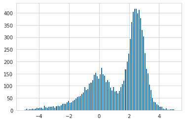
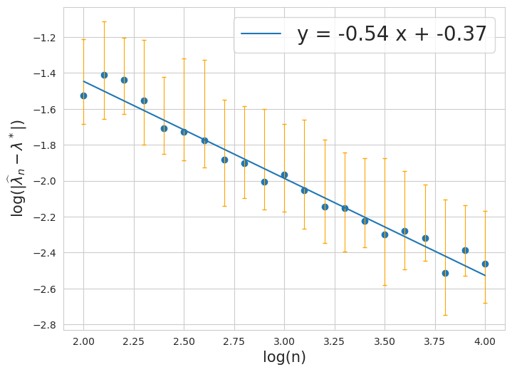
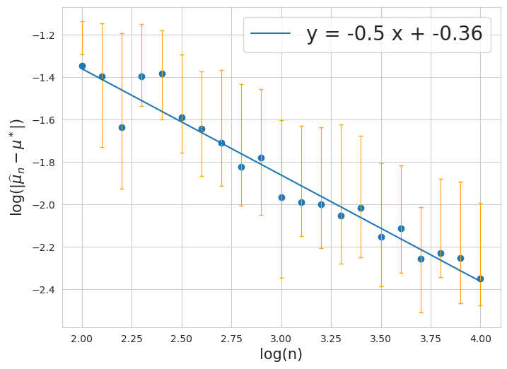
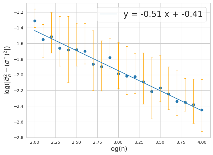
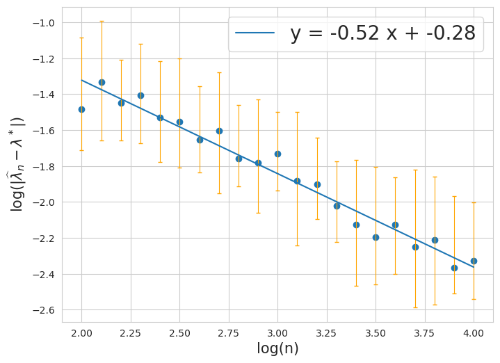
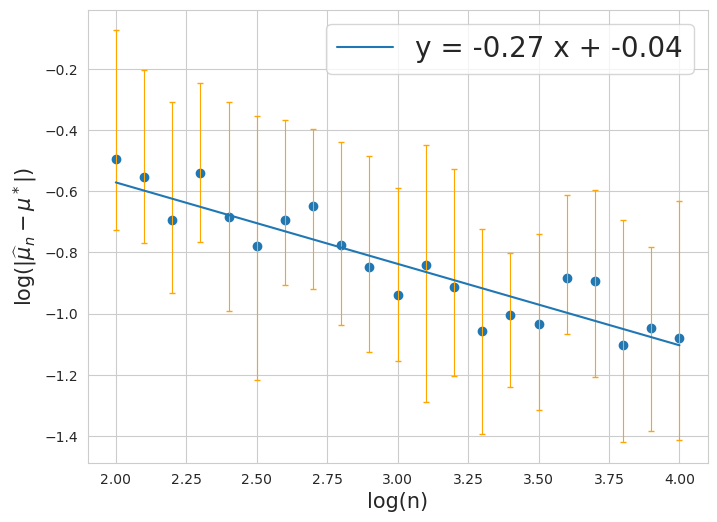
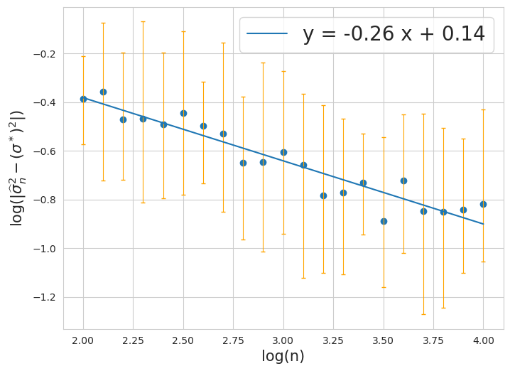
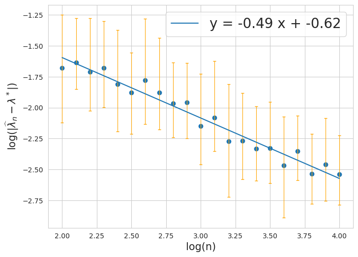
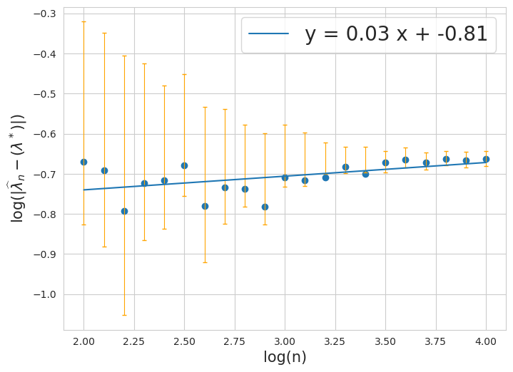
Two histograms for samples from the density pG∗p_{G_{*}} with n=10000n=10000 corresponding to the above two cases are illustrated in Figure 1(a) and  2(a). For each case, we take into account multiple sample sizes nn ranging from 10210^{2} to 10410^{4}. For each sample size nn, we calculate the MLE (λ^n,μ^n,σ^n2)(\hat{\lambda}_{n},\hat{\mu}_{n},\hat{\sigma}^{2}_{n}) via the EM algorithm [13] and measure the errors |λ^n−λ∗||\widehat{\lambda}_{n}-\lambda^{*}|, |μ^n−μ∗||\widehat{\mu}_{n}-\mu^{*}|, and |σ^n2−(σ∗)2||\widehat{\sigma}^{2}_{n}-(\sigma^{*})^{2}|. We repeat this procedure 64 times and plot the mean (blue dot) and quartile error bars (yellow bar) of the logarithm of estimation errors against the log of nn. Theorem 4.1 suggests that the log convergence rate of λ∗\lambda^{*} is of order −1/2{-1/2} for all cases, and so is the rate for (μ,(σ)2)(\mu,(\sigma)^{2}) in the first case. Meanwhile, the convergence rates of (μ∗,(σ∗)2)(\mu^{*},(\sigma^{*})^{2}) in the second case are slower, which is in the order of −1/4{-1/4}. The empirical rates found in the experiments match this theoretical result, where the least square line shows that the logarithm of the rate for estimating μ∗\mu^{*} in case (i) is -0.5 and that of the case (ii) is -0.27 ≈−1/4\approx-1/4 (similar for (σ∗)2(\sigma^{*})^{2}).

(a) Histogram

(a) *
Refer to caption

(b) Rate of λ^n\widehat{\lambda}_{n}

(b) *
Refer to caption

(c) Rate of μ^n\widehat{\mu}_{n}

(c) *
Refer to caption

(d) Rate of σ^n2\widehat{\sigma}^{2}_{n}

(d) *
Refer to caption
Figure 1: Case (i) λ∗=0.5\lambda^{*}=0.5.

(a) Histogram

(a) *
Refer to caption

(b) Rate of λ^n\widehat{\lambda}_{n}

(b) *
Refer to caption

(c) Rate of μ^n\widehat{\mu}_{n}

(c) *
Refer to caption

(d) Rate of σ^n2\widehat{\sigma}^{2}_{n}

(d) *
Refer to caption
Figure 2: Case (ii) λ∗=0.5/n1/4\lambda^{*}=0.5/n^{1/4}.

We once again emphasize that this interesting phenomenon of the rates of convergence is due to the singularity and identifiability of the multivariate deviated model. Our theory and simulation have accurately shown quantitative convergence rates for parameter estimation when λ∗\lambda^{*} near the singularity point 00, where all pairs of (μ∗,Σ∗)(\mu^{*},\Sigma^{*}) in model (2) give the same model. Together with the non-distinguishable settings, we provide a comprehensive study of the large-sample theory for this type of model, thanks to the newly developed notion of distinguishability that helps to control the linear independent relation between h0h_{0} and ff. The developed optimal minimax lower bounds and convergence rates will certainly help Machine Learning practitioners understand better the role of sample sizes in the accuracy of estimation in the multivariate deviated model, and are also inspired theorists to study more about the estimation rate of complex hierarchical/mixture models.

6 Conclusion

In this paper, we establish the uniform rate for estimating true parameters in the multivariate deviated model by using the maximum likelihood estimation (MLE) method. During our derivation, we have to overcome two major obstacles, which are firstly the interaction between the known function h0h_{0} and the Gaussian density ff, and secondly the likelihood of the deviated proportion λ∗\lambda^{*} vanishing to either one or zero. To this end, we introduce a notion of distinguishability to control the linearly independent relation between two functions h0h_{0} and ff. Finally, we achieve the optimal convergence rate of the MLE under both the distinguishable and non-distinguishable settings.

Acknowledgements

NH acknowledges support from the NSF IFML 2019844 and the NSF AI Institute for Foundations of Machine Learning.

References

  • [1] L. Bordes, C. Delmas, and P. Vandekerkhove. Semiparametric estimation of a two-component mixture model where one component is known. Scandinavian journal of statistics, 33(4):733–752, 2006.
  • [2] L. Bordes, S. Mottelet, and P. Vandekerkhove. Semiparametric estimation of a two-component mixture model. The Annals of Statistics, 34(3):1204–1232, 2006.
  • [3] T. Cai, X. J. Jeng, and J. Jin. Optimal detection of heterogeneous and heteroscedastic mixtures. Journal of the Royal Statistical Society: Series B (Statistical Methodology), 73(5):629–662, 2011.
  • [4] T. Cai, J. Jin, and M. G. Low. Estimation and confidence sets for sparse normal mixtures. The Annals of Statistics, 35(6):2421–2449, 2007.
  • [5] T. Cai and Y. Wu. Optimal detection of sparse mixtures against a given null distribution. IEEE Transactions on Information Theory, 60(4):2217 – 2232, 2014.
  • [6] G. Casella and R. L. Berger. Statistical inference. Cengage Learning, 2021.
  • [7] H. Chen and J. Chen. Tests for homogeneity in normal mixtures in the presence of a structural parameter. Statistica Sinica, 13:351–365, 2003.
  • [8] H. Chen, J. Chen, and J. D. Kalbfleisch. A modified likelihood ratio test for homogeneity in finite mixture models. Journal of the Royal Statistical Society: Series B (Statistical Methodology), 63(1):19–29, 2001.
  • [9] J. Chen. Optimal rate of convergence for finite mixture models. Annals of Statistics, 23(1):221–233, 1995.
  • [10] J. Chen, P. Li, and Y. Fu. Inference on the order of a normal mixture. Journal of the American Statistical Association, 107:1096–1105, 2012.
  • [11] W. G. Cochran. The χ\chi2 test of goodness of fit. The Annals of mathematical statistics, pages 315–345, 1952.
  • [12] N. Deb, S. Saha, A. Guntuboyina, and B. Sen. Two-component mixture model in the presence of covariates. Journal of the American Statistical Association, 117(540):1820–1834, 2022.
  • [13] A. P. Dempster, N. M. Laird, and D. B. Rubin. Maximum Likelihood from Incomplete Data Via the EM Algorithm. Journal of the Royal Statistical Society: Series B (Methodological), 39(1):1–22, Sept. 1977.
  • [14] D. Do, N. Ho, and X. Nguyen. Beyond black box densities: Parameter learning for the deviated components. arXiv preprint arXiv:2202.02651, 2022.
  • [15] D. Donoho and J. Jin. Higher criticism for detecting sparse heterogeneous mixtures. Annals of Statistics, 32(3):962–994, 2004.
  • [16] S. Gadat, J. Kahn, C. Marteau, and C. Maugis-Rabusseau. Parameter recovery in two-component contamination mixtures: The l2l^{2} strategy. In Annales de l’Institut Henri Poincaré, Probabilités et Statistiques, volume 56, pages 1391–1418. Institut Henri Poincaré, 2020.
  • [17] E. Giné and R. Nickl. Mathematical foundations of infinite-dimensional statistical models. Cambridge university press, 2021.
  • [18] M. Hardt and E. Price. Tight bounds for learning a mixture of two gaussians. In STOC, 2015.
  • [19] P. Heinrich and J. Kahn. Strong identifiability and optimal minimax rates for finite mixture estimation. Annals of Statistics, 46(6A):2844–2870, 2018.
  • [20] N. Ho and L. Nguyen. Singularity structures and impacts on parameter estimation in finite mixtures of distributions. SIAM Journal on Mathematics of Data Science, 1(4):730–758, 2019.
  • [21] N. Ho and X. Nguyen. Convergence rates of parameter estimation for some weakly identifiable finite mixtures. Annals of Statistics, 44:2726–2755, 2016.
  • [22] N. Ho and X. Nguyen. On strong identifiability and convergence rates of parameter estimation in finite mixtures. Electronic Journal of Statistics, 10:271–307, 2016.
  • [23] E. J. Hu, Y. Shen, P. Wallis, Z. Allen-Zhu, Y. Li, S. Wang, L. Wang, and W. Chen. Lora: Low-rank adaptation of large language models. arXiv preprint arXiv:2106.09685, 2021.
  • [24] H. Kasahara and K. Shimotsu. Non-parametric identification and estimation of the number of components in multivariate mixtures. Journal of the Royal Statistical Society: Series B (Statistical Methodology), 76(1):97–111, 2014.
  • [25] H. Kasahara and K. Shimotsu. Testing the number of components in normal mixture regression models. Journal of the American Statistical Association, 110(512):1632–1645, 2015.
  • [26] P. Li and J. Chen. Testing the order of a finite mixture. Journal of the American Statistical Association, 105(491):1084–1092, 2010.
  • [27] Q. Liu, J. Lee, and M. Jordan. A kernelized stein discrepancy for goodness-of-fit tests. In Proceedings of The 33rd International Conference on Machine Learning, volume 48 of Proceedings of Machine Learning Research, pages 276–284. PMLR, 20–22 Jun 2016.
  • [28] X. Nguyen. Convergence of latent mixing measures in finite and infinite mixture models. Annals of Statistics, 4(1):370–400, 2013.
  • [29] R. Patra and B. Sen. Estimation of a two-component mixture model with applications to multiple testing. J. R. Stat. Soc. Series B Stat. Methodol., 78(4):869–893, 2016.
  • [30] R. Patra and B. Sen. Estimation of a two-component mixture model with applications to multiple testing. Journal of the Royal Statistical Society: Series B (Statistical Methodology), 78(4):869–893, 2016.
  • [31] A. Schrab, B. Guedj, and A. Gretton. KSD aggregated goodness-of-fit test. In A. H. Oh, A. Agarwal, D. Belgrave, and K. Cho, editors, Advances in Neural Information Processing Systems, 2022.
  • [32] S. Talts, M. Betancourt, D. Simpson, A. Vehtari, and A. Gelman. Validating bayesian inference algorithms with simulation-based calibration, 2018.
  • [33] S. van de Geer. Empirical Processes in M-estimation, volume 6. Cambridge university press, 2000.
  • [34] N. Verzelen and E. Arias-Castro. Detection and feature selection in sparse mixture models. Annals of Statistics, 45(5):1920–1950, 2017.
  • [35] C. Villani. Topics in Optimal Transportation. American Mathematical Society, 2003.
  • [36] Y. Wu and P. Yang. Optimal estimation of Gaussian mixtures via denoised method of moments. The Annals of Statistics, 48:1987–2007, 2020.
  • [37] J. Yang, V. Rao, and J. Neville. A stein-papangelou goodness-of-fit test for point processes. In Proceedings of the Twenty-Second International Conference on Artificial Intelligence and Statistics, volume 89 of Proceedings of Machine Learning Research, pages 226–235. PMLR, 16–18 Apr 2019.

In this supplementary material, we present additional results and proofs. The minimax lower bounds and convergence rates of parameter estimation in the non-distinguishable settings are presented in Section A. The general theory for the convergence rates of densities and their proofs can be found in Appendix B. Proofs of the geometric inequalities that relate the convergence of density estimation to that of parameter estimation are in Section C, while those for minimax lower bounds and convergence rates of parameter estimation are left in Appendix D. Then, we provide a necessary lemma for those results along with its proof in Appendix E. Finally, some discussion about the general setting of the paper is presented in Section F, followed by a set of simulations to support the developed theory.

Appendix A Minimax Lower Bounds and Convergence Rates of Parameter Estimation under the Non-distinguishable Settings

Theorem A.1.

(Strongly identifiable and non-distinguishable settings) Assume that classes of densities h0h_{0} and ff satisfy the conditions in Theorem 3.5. We define

Ξ1​(ln):={G=(λ,μ,Σ)∈Ξ:lnmin1≤i≤d11≤u,v≤d2⁡{|(Δ​μ)i|2,|(Δ​Σ)u​v|2}​n≤λ},\displaystyle\Xi_{1}(l_{n}):=\Bigg\{G=(\lambda,\mu,\Sigma)\in\Xi:\dfrac{l_{n}}{\min\limits_{\begin{subarray}{c}1\leq i\leq d_{1}\\ 1\leq u,v\leq d_{2}\end{subarray}}{\left\{|(\Delta\mu)_{i}|^{2},|(\Delta\Sigma)_{uv}|^{2}\right\}}\sqrt{n}}\leq\lambda\Bigg\},

for any sequence {ln}\left\{l_{n}\right\}. Then, we achieve

(a) (Minimax lower bound) Assume that ff satisfies assumption S.1 in Theorem 4.1. Then for any r<1r<1 and sequence {ln}\left\{l_{n}\right\}, there exist two universal positive constants c1c_{1} and c2c_{2} such that

infG^n∈ΞsupG∈Ξ1​(ln)𝔼pG(λ2∥(Δμ,ΔΣ)∥2∥(μ^n,Σ^n)−(μ,Σ)∥2)≥c1n−1/r,\displaystyle\inf\limits_{\widehat{G}_{n}\in\Xi}\sup\limits_{G\in\Xi_{1}(l_{n})}\mathbb{E}_{p_{G}}\biggr(\lambda^{2}\|(\Delta\mu,\Delta\Sigma)\|^{2}\|(\widehat{\mu}_{n},\widehat{\Sigma}_{n})-(\mu,\Sigma)\|^{2}\biggr)\geq c_{1}n^{-1/r},
infG^n∈ΞsupG∈Ξ1​(ln)𝔼pG(∥Δμ,ΔΣ)∥4|λ^n−λ|2)≥c2n−1/r.\displaystyle\inf\limits_{\widehat{G}_{n}\in\Xi}\sup\limits_{G\in\Xi_{1}(l_{n})}\mathbb{E}_{p_{G}}\biggr(\|\Delta\mu,\Delta\Sigma)\|^{4}|\widehat{\lambda}_{n}-\lambda|^{2}\biggr)\geq c_{2}n^{-1/r}.

(b) (MLE rate) Let G^n\widehat{G}_{n} be the MLE defined in equation (3), and the family {pG:G∈Ξ}\{p_{G}:G\in\Xi\} satisfies condition A2. Then, for any sequence {ln}\left\{l_{n}\right\} such that ln/log⁡n→∞l_{n}/\log n\to\infty,

supG∗∈Ξ1​(ln)𝔼pG∗((λ∗)2∥(Δμ∗,ΔΣ∗)∥2∥(μ^n,Σ^n)−(μ∗,Σ∗)∥2)≲log2⁡nn,\displaystyle\sup\limits_{G_{*}\in\Xi_{1}(l_{n})}\mathbb{E}_{p_{G*}}\biggr((\lambda^{*})^{2}\|(\Delta\mu^{*},\Delta\Sigma^{*})\|^{2}\|(\widehat{\mu}_{n},\widehat{\Sigma}_{n})-(\mu^{*},\Sigma^{*})\|^{2}\biggr)\lesssim\dfrac{\log^{2}n}{n},
supG∗∈Ξ1​(ln)𝔼pG∗(∥(Δμ∗,ΔΣ∗)∥4|λ^n−λ∗|2)≲log2⁡nn.\displaystyle\sup\limits_{G_{*}\in\Xi_{1}(l_{n})}\mathbb{E}_{p_{G*}}\biggr(\|(\Delta\mu^{*},\Delta\Sigma^{*})\|^{4}|\widehat{\lambda}_{n}-\lambda^{*}|^{2}\biggr)\lesssim\dfrac{\log^{2}n}{n}.

Proof of Theorem A.1 is in Appendix D.2. The results of part (b) are the generalization of those in Theorem 3.1 and Theorem 3.2 in [16] to the setting of strongly identifiable in the second-order kernel. The condition regarding the lower bound of λ\lambda in the formation of Ξ1​(ln)\Xi_{1}(l_{n}) is necessary to guarantee that (μ^n,Σ^n)(\widehat{\mu}_{n},\widehat{\Sigma}_{n}) and λ^n\widehat{\lambda}_{n} are consistent estimators of (μ∗,Σ∗)(\mu^{*},\Sigma^{*}) and λ∗\lambda^{*} respectively. In particular, from the results in equation (34) of the proof of Theorem A.1, we have for any G∗∈ΞG_{*}\in\Xi that

𝔼pG∗(λ∗)2∥(Δμ∗,ΔΣ∗)∥2∥(μ^n,Σ^n)−(μ∗,Σ∗)∥2≲log2⁡nn.\displaystyle\mathbb{E}_{p_{G*}}(\lambda^{*})^{2}\|(\Delta\mu^{*},\Delta\Sigma^{*})\|^{2}\|(\widehat{\mu}_{n},\widehat{\Sigma}_{n})-(\mu^{*},\Sigma^{*})\|^{2}\lesssim\dfrac{\log^{2}n}{n}.

Therefore, for any 1≤i≤d11\leq i\leq d_{1} and 1≤u,v≤d21\leq u,v\leq d_{2} we get

𝔼pG∗{((Δ​μ^n)i(Δ​μ∗)i−1)2}\displaystyle\mathbb{E}_{p_{G*}}\biggr\{\biggr(\dfrac{(\Delta\widehat{\mu}_{n})_{i}}{(\Delta\mu^{*})_{i}}-1\biggr)^{2}\biggr\} ≲\displaystyle\lesssim log2⁡nn​(λ∗)2​{(Δ​μ∗)i}4,\displaystyle\dfrac{\log^{2}n}{n(\lambda^{*})^{2}\left\{(\Delta\mu^{*})_{i}\right\}^{4}},
𝔼pG∗{((Δ​Σ^n)u​v(Δ​Σ∗)u​v−1)2}\displaystyle\mathbb{E}_{p_{G*}}\biggr\{\biggr(\dfrac{(\Delta\widehat{\Sigma}_{n})_{uv}}{(\Delta\Sigma^{*})_{uv}}-1\biggr)^{2}\biggr\} ≲\displaystyle\lesssim log2⁡nn​(λ∗)2​{(Δ​Σ∗)u​v}4.\displaystyle\dfrac{\log^{2}n}{n(\lambda^{*})^{2}\left\{(\Delta\Sigma^{*})_{uv}\right\}^{4}}.

It indicates that

log⁡nn​λ∗​min1≤i≤d1,1≤u,v≤d2​{|(Δ​μ∗)i|2,|(Δ​Σ∗)i|2}→0\dfrac{\log n}{\sqrt{n}\lambda^{*}\min\limits_{1\leq i\leq d_{1},1\leq u,v\leq d_{2}}\left\{|(\Delta\mu^{*})_{i}|^{2},|(\Delta\Sigma^{*})_{i}|^{2}\right\}}\to 0

for the left-hand-side terms of the above display to go to 0 for all 1≤i≤d11\leq i\leq d_{1} and 1≤u,v≤d21\leq u,v\leq d_{2}.

The results of Theorem A.1 imply that as long as the kernel functions are strongly identifiable in the second order, the convergence rates of μ^n\widehat{\mu}_{n} to μ∗\mu^{*} and Σ^n\widehat{\Sigma}_{n} to Σ∗\Sigma^{*} are similar, which depend on the vanishing rate of (λ∗)2​‖(Δ​μ∗,Δ​Σ∗)‖2(\lambda^{*})^{2}\|(\Delta\mu^{*},\Delta\Sigma^{*})\|^{2} to 0. In our next result of location-covariance multivariate Gaussian distribution, we will demonstrate that such uniform convergence rates of different parameters no longer hold.

Theorem A.2.

(Weakly identifiable and non-distinguishable settings) Assume that ff is a family of location-covariance multivariate Gaussian distributions, and h0​(x)=f⁡(x|μ0,Σ0)h_{0}(x)=f(x|\mu_{0},\Sigma_{0}) for some (μ0,Σ0)∈Θ×Σ(\mu_{0},\Sigma_{0})\in\Theta\times\Sigma. We define

Ξ2​(ln):={G=(λ,μ,Σ)∈Ξ:lnmin1≤i≤d,1≤u,v≤d⁡{|(Δ​μ)i|4,|(Δ​Σ)u​v|2}​n≤λ},\displaystyle\Xi_{2}(l_{n}):=\bigg\{G=(\lambda,\mu,\Sigma)\in\Xi:\dfrac{l_{n}}{\min\limits_{1\leq i\leq d,1\leq u,v\leq d}\left\{|(\Delta\mu)_{i}|^{4},|(\Delta\Sigma)_{uv}|^{2}\right\}\sqrt{n}}\leq\lambda\bigg\},

for any sequence {ln}\left\{l_{n}\right\}. Then, the following holds:

(a) (Minimax lower bound) For any r<1r<1 and sequence {ln}\left\{l_{n}\right\}, there exist two universal positive constants c1c_{1} and c2c_{2} such that

infG^n∈ΞsupG∈Ξ2​(ln)𝔼pG(λ2{∥Δμ∥4+∥ΔΣ∥2}{∥μ^n−μ∥4+∥Σ^n−Σ∥2})≥c1n−1/r,\displaystyle\inf\limits_{\widehat{G}_{n}\in\Xi}\sup\limits_{G\in\Xi_{2}(l_{n})}\mathbb{E}_{p_{G}}\biggr(\lambda^{2}\left\{\|\Delta\mu\|^{4}+\|\Delta\Sigma\|^{2}\right\}\left\{\|\widehat{\mu}_{n}-\mu\|^{4}+\|\widehat{\Sigma}_{n}-\Sigma\|^{2}\right\}\biggr)\geq c_{1}n^{-1/r},
infG^n∈ΞsupG∈Ξ2​(ln)𝔼pG({∥Δμ∥8+∥ΔΣ∥4}|λ^−λ|2)≥c2n−1/r.\displaystyle\inf\limits_{\widehat{G}_{n}\in\Xi}\sup\limits_{G\in\Xi_{2}(l_{n})}\mathbb{E}_{p_{G}}\biggr(\left\{\|\Delta\mu\|^{8}+\|\Delta\Sigma\|^{4}\right\}|\widehat{\lambda}-\lambda|^{2}\biggr)\geq c_{2}n^{-1/r}.

(b) (MLE rate) Let G^n\widehat{G}_{n} be the estimator defined in (3). Then, for any sequence {ln}\left\{l_{n}\right\} such that ln/log⁡n→∞l_{n}/\log n\to\infty the following holds

supG∗∈Ξ2​(ln)𝔼pG∗((λ∗)2{∥Δμ∗∥4+∥ΔΣ∗∥2}{∥μ^n−μ∗∥4+∥Σ^n−Σ∗∥2})≲log2⁡nn,\displaystyle\sup\limits_{G_{*}\in\Xi_{2}(l_{n})}\mathbb{E}_{p_{G*}}\biggr((\lambda^{*})^{2}\left\{\|\Delta\mu^{*}\|^{4}+\|\Delta\Sigma^{*}\|^{2}\right\}\left\{\|\widehat{\mu}_{n}-\mu^{*}\|^{4}+\|\widehat{\Sigma}_{n}-\Sigma^{*}\|^{2}\right\}\biggr)\lesssim\dfrac{\log^{2}n}{n},
supG∗∈Ξ2​(ln)𝔼pG∗({∥Δμ∗∥8+∥ΔΣ∗∥4}|λ^n−λ∗|2)≲log2⁡nn.\displaystyle\sup\limits_{G_{*}\in\Xi_{2}(l_{n})}\mathbb{E}_{p_{G*}}\biggr(\left\{\|\Delta\mu^{*}\|^{8}+\|\Delta\Sigma^{*}\|^{4}\right\}|\widehat{\lambda}_{n}-\lambda^{*}|^{2}\biggr)\lesssim\dfrac{\log^{2}n}{n}.

Proof of Theorem A.2 is in Appendix D.3. A few comments are in order:

(i) Similar to the argument after Theorem A.1, the condition regarding λ\lambda in the formulation of Ξ2​(ln)\Xi_{2}(l_{n}) is to guarantee that (μ^n,Σ^n)(\widehat{\mu}_{n},\widehat{\Sigma}_{n}) and λ^n\widehat{\lambda}_{n} are consistent estimators of (μ∗,Σ∗)(\mu^{*},\Sigma^{*}) and λ∗\lambda^{*}, respectively.

(ii) The results of part (b) indicate that the convergence rate of estimating Σ∗\Sigma^{*} is generally much faster than that of estimating μ∗\mu^{*} regardless of the circumstance of (λ∗)2​{‖Δ​μ∗‖4+‖Δ​Σ∗‖2}(\lambda^{*})^{2}\left\{\|\Delta\mu^{*}\|^{4}+\|\Delta\Sigma^{*}\|^{2}\right\}. The non-uniformity of these convergence rates is mainly due to the structure of the heat partial differential equation, where the second-order derivative of the location parameter and the first-order derivative of covariance parameter correlate.

(iii) From the results of part (b), it is clear that when ‖Δ​μ∗‖+‖Δ​Σ∗‖↛0\|\Delta\mu^{*}\|+\|\Delta\Sigma^{*}\|\not\to 0, i.e., (μ∗,Σ∗)→(μ¯,Σ¯)≠(μ0,Σ0)(\mu^{*},\Sigma^{*})\to(\overline{\mu},\overline{\Sigma})\neq(\mu_{0},\Sigma_{0}), and λ∗↛0\lambda^{*}\not\to 0, the convergence rate of λ^n\widehat{\lambda}_{n} to λ∗\lambda^{*} is n−1/2n^{-1/2}. Furthermore, by using the result from part (a) of Proposition C.4 we can verify that

supG∗𝔼pG∗((λ∗)2{∥μ^n−μ∗∥2+∥Σ^n−Σ∗∥2})≲log2⁡nn,\displaystyle\sup\limits_{G_{*}}\mathbb{E}_{p_{G*}}\biggr((\lambda^{*})^{2}\left\{\|\widehat{\mu}_{n}-\mu^{*}\|^{2}+\|\widehat{\Sigma}_{n}-\Sigma^{*}\|^{2}\right\}\biggr)\lesssim\dfrac{\log^{2}n}{n},

where the supremum is taken over {G∗∈Ξ2​(ln):𝒦⁡(G∗,G¯)≤ϵ}\{G_{*}\in\Xi_{2}(l_{n}):\mathcal{K}(G_{*},\overline{G})\leq\epsilon\}, and G¯=(λ¯,μ¯,Σ¯)\overline{G}=(\overline{\lambda},\overline{\mu},\overline{\Sigma}), λ∗→λ¯\lambda^{*}\to\overline{\lambda}, and ϵ\epsilon is some sufficiently small positive constant. Since λ¯≠0\overline{\lambda}\neq 0, we achieve the optimal convergence rate n−1/2n^{-1/2} of estimating (μ∗,Σ∗)(\mu^{*},\Sigma^{*}) within a sufficiently small neighborhood of G¯\overline{G} under metric 𝒦\mathcal{K}. These results imply that even though the convergence rate of estimating G∗G_{*} may be extremely slow when G∗G_{*} moves over the whole space Ξ2​(ln)\Xi_{2}(l_{n}) (global convergence), such convergence rate can be at standard rate n−1/2n^{-1/2} when G∗G_{*} moves within a sufficiently small neighborhood of some appropriate parameters G¯\overline{G} (local convergence).

As we have seen from the convergence rate results from location-covariance multivariate Gaussian distributions, the heat PDE structure plays a key role in the slow convergence rates of location and covariance parameters as well as the mismatch of orders of these rates.

Appendix B Convergence Rate of Density Estimation

B.1 General Theory and Proof of Theorem 2.3

We now describe the convergence rate of density estimation under the Hellinger distance in detail and give a general result for the multivariate deviated model. We recall some popular notions in Empirical Process theory as follows. An ϵ−\epsilon-net for a metric space (𝒫,d)(\mathcal{P},d) is a collection of balls with radius ϵ\epsilon (with respect to metric dd) having union contains 𝒫\mathcal{P}. The minimal cardinality of such ϵ−\epsilon-nets is called the covering number and denoted by N⁡(ϵ,𝒫,d)N(\epsilon,\mathcal{P},d). The logarithm of N⁡(ϵ,𝒫,d)N(\epsilon,\mathcal{P},d) is called the entropy number and is denoted by H⁡(ϵ,𝒫,d)H(\epsilon,\mathcal{P},d). The bracketing number NB​(ϵ,𝒫,d)N_{B}(\epsilon,\mathcal{P},d) is the minimal number nn such that there exists nn pairs (f¯i,f¯i)i=1n(\underline{f}_{i},\overline{f}_{i})_{i=1}^{n} such that f¯i<f¯i,d⁡(f¯i,f¯i)<ϵ\underline{f}_{i}<\overline{f}_{i},d(\underline{f}_{i},\overline{f}_{i})<\epsilon, and their union covers 𝒫\mathcal{P}. The logarithm of NB​(ϵ,𝒫,d)N_{B}(\epsilon,\mathcal{P},d) is called the bracketing entropy number and is denoted by HB​(ϵ,𝒫,d)H_{B}(\epsilon,\mathcal{P},d). In the following discussion, if 𝒫\mathcal{P} is a family of density and we omit dd, we understand that dd is the distance associated with L2​(m)L^{2}(m), where mm is the Lebesgue measure.

Denote 𝒫⁡(Ξ)={pG:G∈Ξ}\mathcal{P}(\Xi)=\{p_{G}:G\in\Xi\} and 𝒫¯​(Ξ)={(pG∗+pG)/2:G∈Ξ}\overline{\mathcal{P}}(\Xi)=\{(p_{G_{*}}+p_{G})/2:G\in\Xi\} for the fixed true parameter G∗G_{*}. The convergence rate can be deduced from the complexity of the set:

𝒫¯1/2(Ξ,ϵ)={p¯G1/2:G∈Ξ,h(p¯G,pG∗)≤ϵ},\overline{\mathcal{P}}^{1/2}(\Xi,\epsilon)=\left\{\bar{p}_{G}^{1/2}:G\in\Xi,~h(\bar{p}_{G},p_{G_{*}})\leq\epsilon\right\}, (7)

where for any G∈ΞG\in\Xi, we denote p¯G:=(pG+pG∗)/2\bar{p}_{G}:=(p_{G}+p_{G_{*}})/2. We measure the complexity of this class through the bracketing entropy integral

𝒥B​(ϵ,𝒫¯1/2​(Ξ,ϵ))=∫ϵ2/213ϵHB1/2​(u,𝒫¯1/2​(Ξ,ϵ))​𝑑u∨ϵ,\mathcal{J}_{B}(\epsilon,\overline{\mathcal{P}}^{1/2}(\Xi,\epsilon))=\int_{\epsilon^{2}/2^{13}}^{\epsilon}H^{1/2}_{B}(u,\overline{\mathcal{P}}^{1/2}(\Xi,\epsilon))du\vee\epsilon, (8)

where HB​(ϵ,𝒫)H_{B}(\epsilon,\mathcal{P}) denotes the ϵ\epsilon-bracketing entropy number of a metric space 𝒫\mathcal{P}. We recall assumption A2:

  1. A2.

    Given a universal constant J>0J>0, there exists N>0N>0, possibly depending on Θ\Theta and kk, such that for all n≥Nn\geq N and all ϵ>(log⁡n/n)1/2\epsilon>(\log n/n)^{1/2},

    𝒥B​(ϵ,𝒫¯1/2​(Ξ,ϵ))≤J​n​ϵ2.\mathcal{J}_{B}(\epsilon,\overline{\mathcal{P}}^{1/2}(\Xi,\epsilon))\leq J\sqrt{n}\epsilon^{2}.
Theorem B.1.

Assume that Assumption A2 holds, and let k≥1k\geq 1. Then, there exists a constant C>0C>0 depending only on Θ\Theta and kk such that for all n≥1n\geq 1,

supG∗∈Ξ𝔼pG∗​h​(pG^n,pG∗)≤C​log⁡n/n.\sup_{G_{*}\in\Xi}\mathbb{E}_{p_{G_{*}}}h(p_{\widehat{G}_{n}},p_{G_{*}})\leq C\sqrt{\log n/n}.

This result can be obtained by modifying the proof of Theorem 7.4 in [33]. Recall that we defined the function class

𝒫¯1/2(Ξ,ϵ)={p¯G1/2:G∈Ξ,h(p¯G,pG∗)≤ϵ},\overline{\mathcal{P}}^{1/2}(\Xi,\epsilon)=\left\{\bar{p}_{G}^{1/2}:G\in\Xi,~h(\bar{p}_{G},p_{G_{*}})\leq\epsilon\right\}, (9)

where for any G∈ΞG\in\Xi, we write p¯G=(pG+pG∗)/2\bar{p}_{G}=(p_{G}+p_{G_{*}})/2, and measure the complexity of this class through the bracketing entropy integral

𝒥B​(ϵ,𝒫¯1/2​(Ξ,ϵ),ν)=∫ϵ2/213ϵlog⁡NB​(u,𝒫¯1/2​(Ξ,u),ν)​𝑑u∨ϵ,\mathcal{J}_{B}(\epsilon,\overline{\mathcal{P}}^{1/2}(\Xi,\epsilon),\nu)=\int_{\epsilon^{2}/2^{13}}^{\epsilon}\sqrt{\log N_{B}(u,\overline{\mathcal{P}}^{1/2}(\Xi,u),\nu)}du\vee\epsilon,

where NB​(ϵ,X,η)N_{B}(\epsilon,X,\eta) denotes the ϵ\epsilon-bracketing number of a metric space (X,η)(X,\eta) and ν\nu is the Lebesgue measure. We denote by PGP_{G} the distribution corresponding to the density pGp_{G}. The technique to prove this theorem is to bound the convergence rate by the increments of an empirical process:

νn(G)=n∫{pG∗>0}12logp¯GpG∗d(Pn−PG∗),\nu_{n}(G)=\sqrt{n}\int_{\{p_{G_{*}}>0\}}\dfrac{1}{2}\log\dfrac{\overline{p}_{G}}{p_{G_{*}}}d(P_{n}-P_{G_{*}}),

where Pn=1n​∑i=1nδXiP_{n}=\frac{1}{n}\sum_{i=1}^{n}\delta_{X_{i}} is the empirical measure (X1,…,Xn​∼i​i​d​pG∗X_{1},\dots,X_{n}\overset{iid}{\sim}p_{G_{*}}). We first recall Theorem 5.11 in [33] with the notations adapted from our setting:

Theorem B.2.

Let R>0R>0, k≥1k\geq 1, and 𝒢\mathcal{G} be a subset of Ξ\Xi, which contains G∗G_{*}. Given C1<∞C_{1}<\infty, for all CC sufficiently large, and for n∈ℕn\in\mathbb{N} and t>0t>0 satisfying

t≤n​((8​R)∧(C1​R2)),t\leq\sqrt{n}((8R)\wedge(C_{1}R^{2})), (10)

and

t≥C2​(C1+1)​(R∨∫t/(26​n)RHB1/2​(u2,𝒫¯1/2​(Ξ,R),ν)​𝑑u),t\geq C^{2}(C_{1}+1)\left(R\vee\int_{t/(2^{6}\sqrt{n})}^{R}H_{B}^{1/2}\left(\frac{u}{\sqrt{2}},\overline{\mathcal{P}}^{1/2}(\Xi,R),\nu\right)du\right), (11)

we have

ℙλ∗​G∗​(supG∈𝒢,h⁡(p¯G,pG∗)≤R|νn​(G)|≥t)≤C​exp⁡(−t2C2​(C1+1)​R2).\mathbb{P}_{\lambda^{*}G_{*}}\left(\sup_{G\in\mathcal{G},h(\overline{p}_{G},p_{G_{*}})\leq R}|\nu_{n}(G)|\geq t\right)\leq C\exp\left(-\dfrac{t^{2}}{C^{2}(C_{1}+1)R^{2}}\right). (12)

Now we proceed to prove Theorem 2.3, the proof is divided into three parts: Bounding the tail probability of h⁡(pG^n,pG∗)h(p_{\hat{G}_{n}},p_{G_{*}}) by sums of empirical processes increments using the chaining technique, bounding the empirical processes increments using Theorem B.2, and bounding the expectation of h⁡(pG^n,pG∗)h(p_{\hat{G}_{n}},p_{G_{*}}) using its tail probability.

Step 1 (Bounding the tail probability h⁡(pG^n,pG∗)h(p_{\hat{G}_{n}},p_{G_{*}}) by sums of empirical processes increments):

Firstly, by Lemma 4.1 and 4.2 of [33], we have

116​h2​(pG^n,pG∗)≤h2​(p¯G^n,pG∗)≤1n​νn​(G^n).\dfrac{1}{16}h^{2}(p_{\hat{G}_{n}},p_{G_{*}})\leq h^{2}(\overline{p}_{\hat{G}_{n}},p_{G_{*}})\leq\dfrac{1}{\sqrt{n}}\nu_{n}(\hat{G}_{n}).

Hence, for any δ>δn:=(log⁡n/n)1/2\delta>\delta_{n}:=(\log n/n)^{1/2}, we have

ℙG∗​(h⁡(pG^n,pG∗)≥δ)\displaystyle\mathbb{P}_{G_{*}}(h(p_{\hat{G}_{n}},p_{G_{*}})\geq\delta) ≤ℙG∗​(νn​(λ^n​G^n)−n​h2​(p¯G^n,pG∗)≥0CLOSE,\displaystyle\leq\mathbb{P}_{G_{*}}\bigg(\nu_{n}(\hat{\lambda}_{n}\hat{G}_{n})-\sqrt{n}h^{2}(\overline{p}_{\hat{G}_{n}},p_{G_{*}})\geq 0,
OPENh⁡(p¯G^n,pG∗)≥δ/4)\displaystyle\hskip 142.26378pth(\overline{p}_{\hat{G}_{n}},p_{G_{*}})\geq\delta/4\bigg)
≤ℙG∗(supG:h⁡(p¯G,pG∗)≥δ/4[νn(G)−nh2(p¯G,pG∗)]≥0)\displaystyle\leq\mathbb{P}_{G_{*}}\left(\sup_{G:h(\overline{p}_{G},p_{G_{*}})\geq\delta/4}[\nu_{n}(G)-\sqrt{n}h^{2}(\overline{p}_{G},p_{G_{*}})]\geq 0\right)
≤∑s=0SℙG∗(supG:2s​δ/4≤h⁡(p¯G,pG∗)≤2s+1​δ/4|νn(G)|≥n22​s(δ/4)2)\displaystyle\leq\sum_{s=0}^{S}\mathbb{P}_{G_{*}}\left(\sup_{G:2^{s}\delta/4\leq h(\overline{p}_{G},p_{G_{*}})\leq 2^{s+1}\delta/4}|\nu_{n}(G)|\geq\sqrt{n}2^{2s}(\delta/4)^{2}\right)
≤∑s=0SℙG∗(supG:h⁡(p¯G,pG∗)≤2s+1​δ/4|νn(G)|≥n22​s(δ/4)2),\displaystyle\leq\sum_{s=0}^{S}\mathbb{P}_{G_{*}}\left(\sup_{G:h(\overline{p}_{G},p_{G_{*}})\leq 2^{s+1}\delta/4}|\nu_{n}(G)|\geq\sqrt{n}2^{2s}(\delta/4)^{2}\right),

where SS is a smallest number such that 2S​δ/4>12^{S}\delta/4>1, as h⁡(p¯G,pG∗)≤1h(\overline{p}_{G},p_{G_{*}})\leq 1. Now we will bound each term above using Theorem B.2.

Step 2 (Bounding the empirical processes increments using Theorem B.2):

In Theorem B.2, choose R=2s+1​δ,C1=15R=2^{s+1}\delta,C_{1}=15 and t=n​22​s​(δ/4)2t=\sqrt{n}2^{2s}(\delta/4)^{2}, we can readily check that Condition (10) satisfies (because 2s−1​δ/4≤12^{s-1}\delta/4\leq 1 for all s=0,…,Ss=0,\dots,S). Condition (11) satisfies thanks to Assumption A3:

∫t/(26​n)RHB1/2​(u2,𝒫1/2​(Ξ,R),ν)​𝑑u∨2s+1​δ\displaystyle\int_{t/(2^{6}\sqrt{n})}^{R}H_{B}^{1/2}\left(\dfrac{u}{\sqrt{2}},\mathcal{P}^{1/2}(\Xi,R),\nu\right)du\vee 2^{s+1}\delta =2​∫R2/213R/2HB1/2​(u,𝒫1/2​(Ξ,R),ν)​𝑑u∨2s+1​δ\displaystyle=\sqrt{2}\int_{R^{2}/2^{13}}^{R/\sqrt{2}}H_{B}^{1/2}\left(u,\mathcal{P}^{1/2}(\Xi,R),\nu\right)du\vee 2^{s+1}\delta
≤2​𝒥B​(R,𝒫1/2​(Ξ,R),ν)\displaystyle\leq 2\mathcal{J}_{B}(R,\mathcal{P}^{1/2}(\Xi,R),\nu)
≤2​J​n​22​s+1​δ2=26​J​t.\displaystyle\leq 2J\sqrt{n}2^{2s+1}\delta^{2}=2^{6}Jt.

So the conclusion of Theorem B.2 gives us

ℙG∗​(h⁡(pG^n,pG∗)>δ)≤C​∑s=0∞exp⁡(22​s​n​δ2J2​214)≤c​exp⁡(n​δ2c2),\mathbb{P}_{G_{*}}(h(p_{\hat{G}_{n}},p_{G_{*}})>\delta)\leq C\sum_{s=0}^{\infty}\exp\left(\dfrac{2^{2s}n\delta^{2}}{J^{2}2^{14}}\right)\leq c\exp\left(\dfrac{n\delta^{2}}{c^{2}}\right), (13)

where cc is a large constants that does not depend on G∗G_{*}.

Step 3 (Implying the bound on supremum of expectation):

Thus, we have

𝔼​h​(pG^n,pG∗)=∫0∞ℙ⁡(h⁡(pG^n,pG∗)>δ)​𝑑δ≤δn+c​∫δn∞exp⁡(−n​δ2c2)≤c~​δn,\mathbb{E}h(p_{\hat{G}_{n}},p_{G_{*}})=\int_{0}^{\infty}\mathbb{P}(h(p_{\hat{G}_{n}},p_{G_{*}})>\delta)d\delta\leq\delta_{n}+c\int_{\delta_{n}}^{\infty}\exp\left(-\dfrac{n\delta^{2}}{c^{2}}\right)\leq\tilde{c}\delta_{n},

for some c~\tilde{c} does not depend on λ∗,G∗\lambda^{*},G_{*}. Hence, we finally proved that

supG∗∈Ξ𝔼G∗​h​(pG^n,pG∗)≤C​log⁡n/n.\sup_{G_{*}\in\Xi}\mathbb{E}_{G_{*}}h(p_{\widehat{G}_{n}},p_{G_{*}})\leq C\sqrt{\log n/n}.

As a consequence, we obtain the conclusion of the theorem.

B.2 Proof for Proposition 2.4

We further introduce some more notations that are required for the proof. Let N(ϵ,𝒫(Ξ),∥⋅∥∞)N(\epsilon,\mathcal{P}(\Xi),\|\cdot\|_{\infty}) be the ϵ−\epsilon-covering number of (𝒫(Ξ),∥⋅∥∞)(\mathcal{P}(\Xi),\|\cdot\|_{\infty}) and NB​(ϵ,𝒫⁡(Ξ),h)N_{B}(\epsilon,\mathcal{P}(\Xi),h) be the bracketing number of 𝒫⁡(Ξ)\mathcal{P}(\Xi) measured by Hellinger metric hh. HB​(ϵ,𝒫⁡(Ξ),h)=log⁡NB​(ϵ,𝒫⁡(Ξ),h)H_{B}(\epsilon,\mathcal{P}(\Xi),h)=\log N_{B}(\epsilon,\mathcal{P}(\Xi),h) is called the bracketing entropy of 𝒫⁡(Ξ)\mathcal{P}(\Xi) under metric hh. We want to show that

𝒥B​(ϵ,𝒫¯1/2​(Ξ,ϵ),L2​(m))=(∫ϵ2/2213ϵHB1/2​(δ,𝒫¯1/2​(Ξ,δ),L2​(m))​𝑑δ∨δ)≲n​ϵ2,\mathcal{J}_{B}(\epsilon,\overline{\mathcal{P}}^{1/2}(\Xi,\epsilon),L^{2}(m))=\left(\int_{\epsilon^{2}/2^{2^{13}}}^{\epsilon}H_{B}^{1/2}(\delta,\overline{\mathcal{P}}^{1/2}(\Xi,\delta),L^{2}(m))d\delta\vee\delta\right)\lesssim\sqrt{n}\epsilon^{2}, (14)

for all n>Nn>N large enough and ϵ>(log⁡n/n)1/2\epsilon>(\log n/n)^{1/2}. We proceed to show that claim (14) will be proved if

log⁡N⁡(ϵ,𝒫⁡(Ξ),‖⋅‖∞)≲log⁡(1/ϵ),\log N(\epsilon,\mathcal{P}(\Xi),\left\|\cdot\right\|_{\infty})\lesssim\log(1/\epsilon), (15)
HB​(ϵ,𝒫⁡(Ξ),h)≲log⁡(1/ϵ),H_{B}(\epsilon,\mathcal{P}(\Xi),h)\lesssim\log(1/\epsilon), (16)

and then prove claim (15) and (16).

Proof of that claim (16) implies claim (14)

Because 𝒫¯1/2​(Ξ,δ)⊂𝒫¯1/2​(Ξ)\overline{\mathcal{P}}^{1/2}(\Xi,\delta)\subset\overline{\mathcal{P}}^{1/2}(\Xi) and from the definition of Hellinger distance,

HB​(δ,𝒫¯1/2​(Ξ,δ),μ)≤HB​(δ,𝒫¯1/2​(Ξ),μ)=HB​(δ2,𝒫¯​(Ξ),h).H_{B}(\delta,\overline{\mathcal{P}}^{1/2}(\Xi,\delta),\mu)\leq H_{B}(\delta,\overline{\mathcal{P}}^{1/2}(\Xi),\mu)=H_{B}(\frac{\delta}{\sqrt{2}},\overline{\mathcal{P}}(\Xi),h).

Now use the fact that for densities f∗,f1,f2f_{*},f_{1},f_{2}, we have h2​((f1+f∗)/2,(f2+f∗)/2)≤h2​(f1,f2)/2h^{2}((f_{1}+f_{*})/2,(f_{2}+f_{*})/2)\leq h^{2}(f_{1},f_{2})/2, one can readily check that HB​(δ2,𝒫¯​(Ξ),h)≤HB​(δ,𝒫⁡(Ξ),h)H_{B}(\frac{\delta}{\sqrt{2}},\overline{\mathcal{P}}(\Xi),h)\leq H_{B}(\delta,\mathcal{P}(\Xi),h). Hence, if claim (16) holds true, then

HB​(δ,𝒫¯1/2​(Ξ,δ),μ)≤HB​(δ,𝒫⁡(Ξ),h)≲log⁡(1/δ),H_{B}(\delta,\overline{\mathcal{P}}^{1/2}(\Xi,\delta),\mu)\leq H_{B}(\delta,\mathcal{P}(\Xi),h)\lesssim\log(1/\delta),

which implies that

𝒥B​(ϵ,𝒫¯1/2​(Ξ,δ),μ)≲ϵ​(log⁡(213/ϵ2))1/2<n​ϵ2,\mathcal{J}_{B}(\epsilon,\overline{\mathcal{P}}^{1/2}(\Xi,\delta),\mu)\lesssim\epsilon(\log(2^{13}/\epsilon^{2}))^{1/2}<n\epsilon^{2},

for all ϵ>(log⁡n/n)1/2\epsilon>(\log n/n)^{1/2}. Hence, claim (14) is proved.

Proof of claim (15)

As λ∈[0,1]\lambda\in[0,1], we can choose an ϵ−\epsilon-net for it with the cardinality no more than 1ϵ\dfrac{1}{\epsilon}. Similarly, because Θ\Theta and Ω\Omega are compact, we can cover them by hypercube [−a,a]d1[-a,a]^{d_{1}} and [−b,b]d2×d2[-b,b]^{d_{2}\times d_{2}}. Hence, there exists ϵ−\epsilon-nets for them with the cardinality no more than (2​aϵ)d1\left(\dfrac{2a}{\epsilon}\right)^{d_{1}} and (2​bϵ)d22\left(\dfrac{2b}{\epsilon}\right)^{d_{2}^{2}}. Let 𝒮\mathcal{S} be the Cartesian product of them. We have log⁡|𝒮|≲log⁡(1/ϵ)\log|\mathcal{S}|\lesssim\log(1/\epsilon) and for every G=(λ,μ,Σ)∈ΞG=(\lambda,\mu,\Sigma)\in\Xi, there exists G′=(λ′,μ′,Σ′)∈𝒮G^{\prime}=(\lambda^{\prime},\mu^{\prime},\Sigma^{\prime})\in\mathcal{S} such that |λ−λ′|,‖μ−μ′‖,‖Σ−Σ′‖≤ϵ|\lambda-\lambda^{\prime}|,\left\|\mu-\mu^{\prime}\right\|,\left\|\Sigma-\Sigma^{\prime}\right\|\leq\epsilon. By triangle inequalities,

‖pG−pG′‖∞≤|λ−λ′​|(‖h0‖∞+‖f‖∞)+λ|​f​(x|μ,Σ)−f⁡(x|μ′,Σ′)|≲ϵ,\left\|p_{G}-p_{G^{\prime}}\right\|_{\infty}\leq|\lambda-\lambda^{\prime}|(\left\|h_{0}\right\|_{\infty}+\left\|f\right\|_{\infty})+\lambda|f(x|\mu,\Sigma)-f(x|\mu^{\prime},\Sigma^{\prime})|\lesssim\epsilon,

thanks to the uniform bounded and Lipchitz assumptions. Hence,

log⁡N⁡(ϵ,𝒫⁡(Ξ),‖⋅‖∞)≲log⁡(1/ϵ).\log N(\epsilon,\mathcal{P}(\Xi),\left\|\cdot\right\|_{\infty})\lesssim\log(1/\epsilon).
Proof of claim (16)

Now, from the entropy number, we are going to bound the bracketing number, we let η≤ϵ\eta\leq\epsilon which will be chosen later. Let f1,…,fNf_{1},\dots,f_{N} be a η\eta-net for 𝒫⁡(Ξ)\mathcal{P}(\Xi), where fi​(x)=(1−λi)​h0​(x)+λi​f​(x|μi,Σi)f_{i}(x)=(1-\lambda_{i})h_{0}(x)+\lambda_{i}f(x|\mu_{i},\Sigma_{i}). Let

H⁡(x)={b1​exp⁡(−b2​‖x‖b3),‖x‖2≥B1,M,otherwiseH(x)=\begin{cases}b_{1}\exp(-b_{2}\left\|x\right\|^{b_{3}}),&\quad\left\|x\right\|_{2}\geq B_{1},\\ M,&\quad\text{otherwise}\end{cases} (17)

is an envelop for f⁡(x|μ,Σ)f(x|\mu,\Sigma). We can construct brackets [piL,piU][p_{i}^{L},p_{i}^{U}] as follows.

piL​(x)\displaystyle p_{i}^{L}(x) =(1−λi)​h0​(x)+λi​max⁡{f⁡(x|μi,Σi)−η,0},\displaystyle=(1-\lambda_{i})h_{0}(x)+\lambda_{i}\max\{f(x|\mu_{i},\Sigma_{i})-\eta,0\},
piU​(x)\displaystyle p_{i}^{U}(x) =(1−λi)​h0​(x)+λi​min⁡{f⁡(x|μi,Σi)+η,H⁡(x)}.\displaystyle=(1-\lambda_{i})h_{0}(x)+\lambda_{i}\min\{f(x|\mu_{i},\Sigma_{i})+\eta,H(x)\}.

Because for each f∈𝒫⁡(Ξ)f\in\mathcal{P}(\Xi), there is fif_{i} such that ‖f−fi‖∞<η\left\|f-f_{i}\right\|_{\infty}<\eta, we have piL≤f≤piUp_{i}^{L}\leq f\leq p_{i}^{U}. Moreover, for any B¯≥B\overline{B}\geq B,

∫ℝd(piU−piL)​𝑑μ\displaystyle\int_{\mathbb{R}^{d}}(p_{i}^{U}-p_{i}^{L})d\mu ≤λi​(∫‖x‖≤B¯2​η​𝑑x+∫‖x‖≥B¯H⁡(x)​𝑑x)\displaystyle\leq\lambda_{i}\left(\int_{\left\|x\right\|\leq\overline{B}}2\eta dx+\int_{\left\|x\right\|\geq\overline{B}}H(x)dx\right)
≲η​B¯d+B¯d​exp⁡(−b2​B¯b3),\displaystyle\lesssim\eta\overline{B}^{d}+\overline{B}^{d}\exp\left(-b_{2}\overline{B}^{b_{3}}\right), (18)

where we use spherical coordinate to have

∫‖x‖≤B¯𝑑x=πd/2Γ⁡(d/2+1)​B¯d≲B¯d,\int_{\left\|x\right\|\leq\overline{B}}dx=\dfrac{\pi^{d/2}}{\Gamma(d/2+1)}\overline{B}^{d}\lesssim\overline{B}^{d},

and

∫‖x‖≥B¯exp⁡(−b2​‖x‖b3)\displaystyle\int_{\left\|x\right\|\geq\overline{B}}\exp\left(-b_{2}\left\|x\right\|^{b_{3}}\right) ≲∫r≥B¯rd−1​exp⁡(−b2​rb3)​𝑑r\displaystyle\lesssim\int_{r\geq\overline{B}}r^{d-1}\exp\left(-b_{2}r^{b_{3}}\right)dr
=1b3​b21/b3∫B¯b3∞ud/b3−1exp(−u)du(change of variable u=b2rb3)\displaystyle=\dfrac{1}{b_{3}b_{2}^{1/b_{3}}}\int_{\overline{B}^{b_{3}}}^{\infty}u^{d/b_{3}-1}\exp(-u)du\quad(\text{change of variable }u=b_{2}r^{b_{3}})
≤1b3​b21/b3​B¯d−b3​exp⁡(−B¯b3).\displaystyle\leq\dfrac{1}{b_{3}b_{2}^{1/b_{3}}}\overline{B}^{d-b_{3}}\exp(-\overline{B}^{b_{3}}).

Hence, in (18), if we choose B¯=B​(log⁡(1/η))1/b3\overline{B}=B(\log(1/\eta))^{1/b_{3}} then

∫ℝd(piU−piL)​𝑑μ≲η​(log⁡(1η))d/b3.\int_{\mathbb{R}^{d}}(p_{i}^{U}-p_{i}^{L})d\mu\lesssim\eta\left(\log\left(\dfrac{1}{\eta}\right)\right)^{d/b_{3}}. (19)

Therefore, there exists a positive constant cc which does not depend on η\eta such that

HB​(c​η​log⁡(1/η)d/b3,𝒫⁡(Ξ),‖⋅‖1)≲log⁡(1/η).H_{B}(c\eta\log(1/\eta)^{d/b_{3}},\mathcal{P}(\Xi),\left\|\cdot\right\|_{1})\lesssim\log(1/\eta).

Let ϵ=c​η​(log⁡(1/η))d/b3\epsilon=c\eta(\log(1/\eta))^{d/b_{3}}, we have log⁡(1/ϵ)≍log⁡(1/η)\log(1/\epsilon)\asymp\log(1/\eta), which combines with inequality ‖⋅‖1≤h2\left\|\cdot\right\|_{1}\leq h^{2} leads to

HB​(ϵ,𝒫⁡(Ξ),h)≤HB​(ϵ2,𝒫⁡(Ξ),‖⋅‖1)≲log⁡(1/ϵ2)≲log⁡(1/ϵ).H_{B}(\epsilon,\mathcal{P}(\Xi),h)\leq H_{B}(\epsilon^{2},\mathcal{P}(\Xi),\left\|\cdot\right\|_{1})\lesssim\log(1/\epsilon^{2})\lesssim\log(1/\epsilon).

Thus, we have proved claim (16).

Appendix C Proofs for Geometric Inverse Bounds

C.1 Proof of Theorem 3.3

The second inequality in Theorem 3.3 is straightforward from the equivalent form of W1​(G,G∗)W_{1}(G,G_{*}) in Lemma E.1 (see Appendix E). Therefore, we will only focus on establishing the first inequality in that theorem. We start with the following key result:

Proposition C.1.

Given the assumptions in Theorem 3.5 and G¯=(λ¯,μ¯,Σ¯)\overline{G}=(\overline{\lambda},\overline{\mu},\overline{\Sigma}) such that λ¯∈[0,1]\overline{\lambda}\in[0,1] and (μ¯,Σ¯)(\overline{\mu},\overline{\Sigma}) can be equal to (μ0,Σ0)(\mu_{0},\Sigma_{0}). Then, we have

limϵ→0infG,G∗{V⁡(pG,pG∗)𝒦⁡(G,G∗):𝒦⁡(G,G¯)∨𝒦⁡(G∗,G¯)≤ϵ}>0.\displaystyle\lim\limits_{\epsilon\to 0}\inf\limits_{G,G_{*}}{\left\{\dfrac{V(p_{G},p_{G_{*}})}{\mathcal{K}(G,G_{*})}:\ \mathcal{K}(G,\overline{G})\vee\mathcal{K}(G_{*},\overline{G})\leq\epsilon\right\}}>0.
Proof.

The high level idea of the proof of Proposition C.3 is to utilize the Taylor expansion techniques previously employed in [9, 28, 22, 19]. Indeed, following Fatou’s argument from Theorem 3.1 in [22], to obtain the conclusion of Proposition C.3 it suffices to demonstrate that

limϵ→0infG,G∗{‖pG−pG∗‖∞𝒦⁡(G,G∗):𝒦⁡(G,G¯)∨𝒦⁡(G∗,G¯)≤ϵ}>0.\displaystyle\lim\limits_{\epsilon\to 0}\inf\limits_{G,G_{*}}{\left\{\dfrac{\|p_{G}-p_{G_{*}}\|_{\infty}}{\mathcal{K}(G,G_{*})}:\ \mathcal{K}(G,\overline{G})\vee\mathcal{K}(G_{*},\overline{G})\leq\epsilon\right\}}>0.

Assume that the above conclusion does not hold. It implies that we can find two sequences Gn=(λn,μn,Σn)G_{n}=(\lambda_{n},\mu_{n},\Sigma_{n}) and G∗,n=(λn∗,μn∗,Σn∗)G_{*,n}=(\lambda^{*}_{n},\mu_{n}^{*},\Sigma_{n}^{*}) such that 𝒦⁡(Gn,G¯)→0\mathcal{K}(G_{n},\overline{G})\to 0, 𝒦⁡(G∗,n,G¯)→0\mathcal{K}(G_{*,n},\overline{G})\to 0, and ‖pGn−pG∗,n‖∞/𝒦⁡(Gn,G∗,n)→0\|p_{G_{n}}-p_{G_{*,n}}\|_{\infty}/\mathcal{K}(G_{n},G_{*,n})\to 0 as n→∞n\to\infty. Now, we only consider the most challenging setting of (μn,Σn)(\mu_{n},\Sigma_{n}) and (μn∗,Σn∗)(\mu_{n}^{*},\Sigma_{n}^{*}) when they share the same limit point (μ′,Σ′)(\mu^{\prime},\Sigma^{\prime}). The other settings of these two components can be argued in the same fashion. Here, (μ′,Σ′)(\mu^{\prime},\Sigma^{\prime}) is not necessarily equal to (μ0,Σ0)(\mu_{0},\Sigma_{0}) or (μ¯,Σ¯)(\overline{\mu},\overline{\Sigma}) as λn,λn∗\lambda_{n},\lambda_{n}^{*} can go to 0 or 1 in the limit. Under that setting, by means of Taylor expansion up to the first order we obtain

pGn​(x)−pG∗,n​(x)𝒦⁡(Gn,G∗,n)\displaystyle\dfrac{p_{G_{n}}(x)-p_{G_{*,n}}(x)}{\mathcal{K}(G_{n},G_{*,n})} =\displaystyle= (λn∗−λn)​[h0​(x|μ0,Σ0)−f⁡(x|μn∗,Σn∗)]+λn​[f⁡(x|μn,Σn)−f⁡(x|μn∗,Σn∗)]𝒦⁡(Gn,G∗,n)\displaystyle\dfrac{(\lambda^{*}_{n}-\lambda_{n})[h_{0}(x|\mu_{0},\Sigma_{0})-f(x|\mu_{n}^{*},\Sigma_{n}^{*})]+\lambda_{n}[f(x|\mu_{n},\Sigma_{n})-f(x|\mu^{*}_{n},\Sigma^{*}_{n})]}{\mathcal{K}(G_{n},G_{*,n})}
=\displaystyle= (λn∗−λn)​[h0​(x|μ0,Σ0)−f⁡(x|μn∗,Σn∗)]𝒦⁡(Gn,G∗,n)\displaystyle\dfrac{(\lambda^{*}_{n}-\lambda_{n})[h_{0}(x|\mu_{0},\Sigma_{0})-f(x|\mu_{n}^{*},\Sigma_{n}^{*})]}{\mathcal{K}(G_{n},G_{*,n})}
+\displaystyle+ λn(∑|α|=1(μn−μn∗)α1​(Σn−Σn∗)α2α!∂|α|f∂μα1​∂Σα2(x|μn∗,Σn∗)+R1(x))𝒦⁡(Gn,G∗,n)\displaystyle\dfrac{\lambda_{n}\biggr(\sum\limits_{|\alpha|=1}\dfrac{(\mu_{n}-\mu^{*}_{n})^{\alpha_{1}}(\Sigma_{n}-\Sigma^{*}_{n})^{\alpha_{2}}}{\alpha!}\dfrac{\partial^{|\alpha|}{f}}{\partial{\mu^{\alpha_{1}}}\partial{\Sigma^{\alpha_{2}}}}(x|\mu_{n}^{*},\Sigma_{n}^{*})+R_{1}(x)\biggr)}{\mathcal{K}(G_{n},G_{*,n})}

where R1​(x)R_{1}(x) is Taylor remainder and α=(α1,α2)\alpha=(\alpha_{1},\alpha_{2}) in the summation of the second equality satisfies α1=(α1(1),…,αd1(1))∈ℕd1\alpha_{1}=(\alpha_{1}^{(1)},\ldots,\alpha_{d_{1}}^{(1)})\in\mathbb{N}^{d_{1}}, α2=(αu​v(2))∈ℕd2×d2\alpha_{2}=(\alpha_{uv}^{(2)})\in\mathbb{N}^{d_{2}\times d_{2}}, |α|=∑i=1d1αi(1)+∑1≤u,v≤d2αu​v(2)|\alpha|=\sum\limits_{i=1}^{d_{1}}{\alpha_{i}^{(1)}}+\sum\limits_{1\leq u,v\leq d_{2}}{\alpha_{uv}^{(2)}}, and α!=∏i=1d1αi(1)!​∏1≤u,v≤d2αu​v(2)!\alpha!=\prod\limits_{i=1}^{d_{1}}{\alpha_{i}^{(1)}!}\prod\limits_{1\leq u,v\leq d_{2}}{\alpha_{uv}^{(2)}!}. As ff admits the first order uniform Lipschitz condition, we have R1​(x)=O⁡(‖(μn,Σn)−(μn∗,Σn∗)‖1+γ)R_{1}(x)=O(\|(\mu_{n},\Sigma_{n})-(\mu_{n}^{*},\Sigma_{n}^{*})\|^{1+\gamma}) for some γ>0\gamma>0, which implies that

λn​|R1​(x)|/𝒦⁡(Gn,G∗,n)=O⁡(‖(μn,Σn)−(μn∗,Σn∗)‖γ)→0\displaystyle\lambda_{n}|R_{1}(x)|/\mathcal{K}(G_{n},G_{*,n})=O(\|(\mu_{n},\Sigma_{n})-(\mu_{n}^{*},\Sigma_{n}^{*})\|^{\gamma})\to 0

as n→∞n\to\infty. Therefore, we can treat [pGn​(x)−pG∗,n​(x)]/𝒦⁡(Gn,G∗,n)[p_{G_{n}}(x)-p_{G_{*,n}}(x)]/\mathcal{K}(G_{n},G_{*,n}) as the linear combination of h0​(x|θ0,Σ0)h_{0}(x|\theta_{0},\Sigma_{0}) and ∂|α|f∂μα1​∂Σα2​(x|μn∗,Σn∗)\dfrac{\partial^{|\alpha|}{f}}{\partial{\mu^{\alpha_{1}}}\partial{\Sigma^{\alpha_{2}}}}(x|\mu_{n}^{*},\Sigma_{n}^{*}) when |α|≤1|\alpha|\leq 1. Assume that the coefficients of these terms go to 0. Then, by studying the coefficients of h0​(x|θ0,Σ0)h_{0}(x|\theta_{0},\Sigma_{0}), ∂f∂μi​(x|μ0,Σ0)\dfrac{\partial{f}}{\partial{\mu_{i}}}(x|\mu_{0},\Sigma_{0}), and ∂f∂Σu​v​(x|μ0,Σ0)\dfrac{\partial{f}}{\partial{\Sigma_{uv}}}(x|\mu_{0},\Sigma_{0}), we achieve

(λn∗−λn)/𝒦⁡(Gn,G∗,n)→0,λn​(μn−μn∗)i/𝒦⁡(Gn,G∗,n)→0,λn​(Σn−Σn∗)u​v/𝒦⁡(Gn,G∗,n)→0\displaystyle(\lambda_{n}^{*}-\lambda_{n})/\mathcal{K}(G_{n},G_{*,n})\to 0,\ \lambda_{n}(\mu_{n}-\mu_{n}^{*})_{i}/\mathcal{K}(G_{n},G_{*,n})\to 0,\ \lambda_{n}(\Sigma_{n}-\Sigma_{n}^{*})_{uv}/\mathcal{K}(G_{n},G_{*,n})\to 0

for all 1≤i≤d11\leq i\leq d_{1} and 1≤u,v≤d21\leq u,v\leq d_{2} where (a)i(a)_{i} denotes the ii-th element of vector aa and Au​vA_{uv} denotes the (u,v)(u,v)-th element of matrix AA. It would imply that

(λn+λn∗)​‖(μn,Σn)−(μn∗,Σn∗)‖/𝒦⁡(Gn,G∗,n)→0.\displaystyle(\lambda_{n}+\lambda_{n}^{*})\|(\mu_{n},\Sigma_{n})-(\mu_{n}^{*},\Sigma_{n}^{*})\|/\mathcal{K}(G_{n},G_{*,n})\to 0.

Therefore, we achieve

1=(|λn∗−λn|+(λn+λn∗)∥(μn,Σn)−(μn∗,Σn∗)∥)/𝒦(Gn,G∗,n)→0,\displaystyle 1=\biggr(|\lambda_{n}^{*}-\lambda_{n}|+(\lambda_{n}+\lambda_{n}^{*})\|(\mu_{n},\Sigma_{n})-(\mu_{n}^{*},\Sigma_{n}^{*})\|\biggr)/\mathcal{K}(G_{n},G_{*,n})\to 0,

a contradiction. Therefore, not all the coefficients of h0​(x|θ0,Σ0)h_{0}(x|\theta_{0},\Sigma_{0}) and ∂|α|f∂μα1​∂Σα2​(x|μn∗,Σn∗)\dfrac{\partial^{|\alpha|}{f}}{\partial{\mu^{\alpha_{1}}}\partial{\Sigma^{\alpha_{2}}}}(x|\mu_{n}^{*},\Sigma_{n}^{*}) go to 0. If we denote mnm_{n} to be the maximum of the absolute values of the coefficients of h0​(x|θ0,Σ0)h_{0}(x|\theta_{0},\Sigma_{0}) and ∂|α|f∂μα1​∂Σα2​(x|μn∗,Σn∗)\dfrac{\partial^{|\alpha|}{f}}{\partial{\mu^{\alpha_{1}}}\partial{\Sigma^{\alpha_{2}}}}(x|\mu_{n}^{*},\Sigma_{n}^{*}), then we get 1/mn↛∞1/m_{n}\not\to\infty as n→∞n\to\infty, i.e., 1/mn1/m_{n} is uniformly bounded. Hence, we achieve for all xx that

1mnpGn​(x)−pG∗,n​(x)K⁡(Gn,G∗,n)→ηf(|μ0,Σ0)+∑|α|≤1τα∂|α|f∂μα1​∂Σα2(x|μ′,Σ′)=0\displaystyle\dfrac{1}{m_{n}}\dfrac{p_{G_{n}}(x)-p_{G_{*,n}}(x)}{K(G_{n},G_{*,n})}\to\eta f(|\mu_{0},\Sigma_{0})+\sum\limits_{|\alpha|\leq 1}{\tau_{\alpha}\dfrac{\partial^{|\alpha|}{f}}{\partial{\mu^{\alpha_{1}}}\partial{\Sigma^{\alpha_{2}}}}(x|\mu^{\prime},\Sigma^{\prime})}=0

for some coefficients η\eta and τα\tau_{\alpha} such that they are not all 0. However, as ff is distinguishable from h0h_{0} up to the first order, the above equation indicates that η=τα=0\eta=\tau_{\alpha}=0 for all |α|≤1|\alpha|\leq 1, a contradiction. As a consequence, we achieve the conclusion of the proposition. ∎

Now, assume that the conclusion of Theorem (3.3) does not hold. It implies that we can find two sequences Gn′G_{n}^{\prime} and G∗,n′G_{*,n}^{\prime} such that An=‖pGn′−pG∗,n′‖2/𝒦⁡(Gn′,G∗,n′)→0A_{n}=\|p_{G_{n}^{\prime}}-p_{G_{*,n}^{\prime}}\|_{2}/\mathcal{K}(G_{n}^{\prime},G_{*,n}^{\prime})\to 0 as n→∞n\to\infty. Since Θ\Theta and Ω\Omega are two bounded subsets, we can find subsequences of Gn′G_{n}^{\prime} and G∗,n′G_{*,n}^{\prime} such that 𝒦⁡(Gn′,G¯1)\mathcal{K}(G_{n}^{\prime},\overline{G}_{1}) and 𝒦⁡(G∗,n′,G¯2)\mathcal{K}(G_{*,n}^{\prime},\overline{G}_{2}) vanish to 0 as n→∞n\to\infty where G¯1,G¯2\overline{G}_{1},\overline{G}_{2} are some discrete measures having one component to be (μ0,Σ0)(\mu_{0},\Sigma_{0}). Because An→0A_{n}\to 0, we obtain V⁡(pGn′,pG∗,n′)→0V(p_{G_{n}^{\prime}},p_{G_{*,n}^{\prime}})\to 0 as n→∞n\to\infty. By means of Fatou’s lemma, we have

0=limn→∞∫|(pGn′​(x)−pG∗,n′​(x))|​𝑑x≥∫lim infn→∞|(pGn′​(x)−pG∗,n′​(x))|​𝑑x=V⁡(pG¯1​(x),pG¯2​(x)).\displaystyle 0=\lim\limits_{n\to\infty}\int\left|(p_{G_{n}^{\prime}}(x)-p_{G_{*,n}^{\prime}}(x))\right|dx\geq\int\mathop{\liminf}\limits_{n\to\infty}\left|(p_{G_{n}^{\prime}}(x)-p_{G_{*,n}^{\prime}}(x))\right|dx=V(p_{\overline{G}_{1}}(x),p_{\overline{G}_{2}}(x)).

Due to the fact that ff is distinguishable from h0h_{0} up to the first order, the above equation implies that G¯1≡G¯2\overline{G}_{1}\equiv\overline{G}_{2}. However, from the result of Proposition C.1, regardless of the value of G¯1\overline{G}_{1} we would have An↛0A_{n}\not\to 0 as n→∞n\to\infty, which is a contradiction. Therefore, we obtain the conclusion of the theorem.

C.2 Proof of Theorem 3.5

Prior to presenting the proof of Theorem 3.5, we introduce the definition of second-order uniform Lipschitz:

Definition C.2 (Second-order Uniform Lipschitz).

We say that ff is uniformly Lipschitz up to the second order if the following holds: there are positive constants δ3\delta_{3}, δ4\delta_{4} such that for any R4,R5,R6>0R_{4},R_{5},R_{6}>0, γ1∈ℝd1\gamma_{1}\in\mathbb{R}^{d_{1}}, γ2∈ℝd2×d2\gamma_{2}\in\mathbb{R}^{d_{2}\times d_{2}}, R4≤λ1​(Σ)≤λd2​(Σ)≤R5R_{4}\leq\sqrt{\lambda_{1}(\Sigma)}\leq\sqrt{\lambda_{d_{2}}(\Sigma)}\leq R_{5}, ‖θ‖≤R6\|\theta\|\leq R_{6}, θ1,θ2∈Θ\theta_{1},\theta_{2}\in\Theta, Σ1,Σ2∈Ω\Sigma_{1},\Sigma_{2}\in\Omega, there are positive constants C1C_{1} depending on (R4,R5)(R_{4},R_{5}) and C2C_{2} depending on R6R_{6} such that for all x∈𝒳x\in\mathcal{X},

|γ1⊤​(∂2f∂θ2​(x|θ1,Σ)−∂2f∂θ2​(x|θ2,Σ))​γ1|≤‖θ1−θ2‖1δ3​‖γ1‖22,\displaystyle\Big|\gamma_{1}^{\top}\Big(\frac{\partial^{2}f}{\partial\theta^{2}}(x|\theta_{1},\Sigma)-\frac{\partial^{2}f}{\partial\theta^{2}}(x|\theta_{2},\Sigma)\Big)\gamma_{1}\Big|\leq\|\theta_{1}-\theta_{2}\|_{1}^{\delta_{3}}\|\gamma_{1}\|_{2}^{2},
|tr⁡([∂∂Σ​(tr⁡(∂f∂Σ1​(x|θ,Σ)⊤​γ2))−∂∂Σ​(tr⁡(∂f∂Σ​(x|θ,Σ2)⊤​γ2))]⊤​γ2)|\displaystyle\Big|\operatorname{tr}\Big(\Big[\frac{\partial}{\partial\Sigma}\Big(\operatorname{tr}\Big(\frac{\partial f}{\partial\Sigma_{1}}(x|\theta,\Sigma)^{\top}\gamma_{2}\Big)\Big)-\frac{\partial}{\partial\Sigma}\Big(\operatorname{tr}\Big(\frac{\partial f}{\partial\Sigma}(x|\theta,\Sigma_{2})^{\top}\gamma_{2}\Big)\Big)\Big]^{\top}\gamma_{2}\Big)\Big|
≤C2​‖Σ1−Σ2‖2δ4​‖γ‖22.\displaystyle\leq C_{2}\|\Sigma_{1}-\Sigma_{2}\|_{2}^{\delta_{4}}\|\gamma\|_{2}^{2}.

Now, we are back to the main proof. Utilizing the same Fatou’s argument as that of Proposition C.1 , to achieve the conclusion of the first inequality in Theorem 3.5 it suffices to demonstrate the following result

Proposition C.3.

Given the assumptions in Theorem 3.5 and G¯=(λ¯,μ¯,Σ¯)\overline{G}=(\overline{\lambda},\overline{\mu},\overline{\Sigma}) such that λ¯∈[0,1]\overline{\lambda}\in[0,1] and (μ¯,Σ¯)(\overline{\mu},\overline{\Sigma}) can be identical to (μ0,Σ0)(\mu_{0},\Sigma_{0}). Then, the following holds

  • (a)

    If (μ0,Σ0)≠(μ¯,Σ¯)(\mu_{0},\Sigma_{0})\neq(\overline{\mu},\overline{\Sigma}) and λ¯>0\overline{\lambda}>0, then

    limϵ→0infG,G∗{‖pG−pG∗‖∞𝒦⁡(G,G∗):𝒦⁡(G,G¯)∨𝒦⁡(G∗,G¯)≤ϵ}>0.\displaystyle\lim\limits_{\epsilon\to 0}\inf\limits_{G,G_{*}}{\left\{\dfrac{\|p_{G}-p_{G_{*}}\|_{\infty}}{\mathcal{K}(G,G_{*})}:\ \mathcal{K}(G,\overline{G})\vee\mathcal{K}(G_{*},\overline{G})\leq\epsilon\right\}}>0.
  • (b)

    If (μ0,Σ0)≡(μ¯,Σ¯)(\mu_{0},\Sigma_{0})\equiv(\overline{\mu},\overline{\Sigma}) or (μ0,Σ0)≠(μ¯,Σ¯)(\mu_{0},\Sigma_{0})\neq(\overline{\mu},\overline{\Sigma}) and λ¯=0\overline{\lambda}=0, then

    limϵ→0infG,G∗{‖pG−pG∗‖∞𝒟⁡(G,G∗):𝒟⁡(G,G¯)∨𝒟⁡(G∗,G¯)≤ϵ}>0.\displaystyle\lim\limits_{\epsilon\to 0}\inf\limits_{G,G_{*}}{\left\{\dfrac{\|p_{G}-p_{G_{*}}\|_{\infty}}{\mathcal{D}(G,G_{*})}:\ \mathcal{D}(G,\overline{G})\vee\mathcal{D}(G_{*},\overline{G})\leq\epsilon\right\}}>0.
Proof.

The proof of part (a) is essentially similar to that of Proposition C.1; therefore, we only provide the proof for the challenging settings of part (b). Here, we only consider the setting that (μ0,Σ0)≡(μ¯,Σ¯)(\mu_{0},\Sigma_{0})\equiv(\overline{\mu},\overline{\Sigma}) as the proof for other possibilities of (μ0,Σ0)(\mu_{0},\Sigma_{0}) can be argued in the similar fashion. Under this assumption, (μ0,Σ0)=(μ0,Σ0)(\mu_{0},\Sigma_{0})=(\mu_{0},\Sigma_{0}), G¯=(λ¯,θ0,Σ0)\overline{G}=(\overline{\lambda},\theta_{0},\Sigma_{0}), and h0​(x|θ0,Σ0)=f⁡(x|θ0,Σ0)h_{0}(x|\theta_{0},\Sigma_{0})=f(x|\theta_{0},\Sigma_{0}) for all x∈𝒳x\in\mathcal{X}. Assume that the conclusion of Proposition C.3 does not hold. It implies that we can find two sequences Gn=(λn,μn,Σn)G_{n}=(\lambda_{n},\mu_{n},\Sigma_{n}) and G∗,n=(λn∗,μn∗,Σn∗)G_{*,n}=(\lambda^{*}_{n},\mu^{*}_{n},\Sigma_{n}^{*}) such that 𝒟⁡(Gn,G¯)=λn​‖(Δ​μn,Δ​Σn)‖2→0\mathcal{D}(G_{n},\overline{G})=\lambda_{n}\|(\Delta\mu_{n},\Delta\Sigma_{n})\|^{2}\to 0, 𝒟⁡(G∗,n,G¯)=λn∗​‖(Δ​μn∗,Δ​Σn∗)‖2→0\mathcal{D}(G_{*,n},\overline{G})=\lambda_{n}^{*}\|(\Delta\mu_{n}^{*},\Delta\Sigma_{n}^{*})\|^{2}\to 0, and ‖pGn−pG∗,n‖∞/𝒟⁡(Gn,G∗,n)→0\|p_{G_{n}}-p_{G_{*,n}}\|_{\infty}/\mathcal{D}(G_{n},G_{*,n})\to 0 as n→∞n\to\infty. For the transparency of presentation, we denote An=‖(Δ​μn,Δ​Σn)‖A_{n}=\|(\Delta\mu_{n},\Delta\Sigma_{n})\|, Bn=‖(Δ​μn∗,Δ​Σn∗)‖B_{n}=\|(\Delta\mu_{n}^{*},\Delta\Sigma_{n}^{*})\|, and Cn=|(μn,Σn)−(μn∗,Σn∗)|=‖(Δ​μn,Δ​Σn)−(Δ​μn∗,Δ​Σn∗)‖C_{n}=\|(\mu_{n},\Sigma_{n})-(\mu_{n}^{*},\Sigma_{n}^{*})\|=\|(\Delta\mu_{n},\Delta\Sigma_{n})-(\Delta\mu_{n}^{*},\Delta\Sigma_{n}^{*})\|. Now, we have three main cases regarding the convergence behaviors of (μn,Σn)(\mu_{n},\Sigma_{n}) and (μn∗,Σn∗)(\mu^{*}_{n},\Sigma^{*}_{n})

Case 1:

Both An→0A_{n}\to 0 and Bn→0B_{n}\to 0, i.e., (μn,Σn)(\mu_{n},\Sigma_{n}) and (μn∗,Σn∗)(\mu^{*}_{n},\Sigma^{*}_{n}) vanish to (μ0,Σ0)(\mu_{0},\Sigma_{0}) as n→∞n\to\infty. Due to the symmetry between λn\lambda_{n} and λn∗\lambda_{n}^{*}, we assume without loss of generality that λn∗≥λn\lambda_{n}^{*}\geq\lambda_{n} for infinite values of nn. Without loss of generality, we replace these subsequences of Gn,G∗,nG_{n},G_{*,n} by the whole sequences of GnG_{n} and G∗,nG_{*,n}. Now, the formulation of 𝒟⁡(Gn,G∗,n)\mathcal{D}(G_{n},G_{*,n}) is

𝒟(Gn,G∗,n)=(λn∗−λn)Bn2+(λnAn+λn∗Bn)Cn.\displaystyle\mathcal{D}(G_{n},G_{*,n})=(\lambda_{n}^{*}-\lambda_{n})B_{n}^{2}+\biggr(\lambda_{n}A_{n}+\lambda_{n}^{*}B_{n}\biggr)C_{n}.

Now, by means of Taylor expansion up to the second order, we get

pGn​(x)−pG∗,n​(x)𝒟⁡(Gn,G∗,n)\displaystyle\dfrac{p_{G_{n}}(x)-p_{G_{*,n}}(x)}{\mathcal{D}(G_{n},G_{*,n})} =\displaystyle= (λn∗−λn)​[f⁡(x|μ0,Σ0)−f⁡(x|μn∗,Σn∗)]+λn​[f⁡(x|μn,Σn)−f⁡(x|μn∗,Σn∗)]𝒟⁡(Gn,G∗,n)\displaystyle\dfrac{(\lambda^{*}_{n}-\lambda_{n})[f(x|\mu_{0},\Sigma_{0})-f(x|\mu_{n}^{*},\Sigma_{n}^{*})]+\lambda_{n}[f(x|\mu_{n},\Sigma_{n})-f(x|\mu^{*}_{n},\Sigma^{*}_{n})]}{\mathcal{D}(G_{n},G_{*,n})}
=\displaystyle= (λ∗n−λn)(∑|α|=12(−Δ​μn∗)α1​(−Δ​Σn∗)α2α!∂|α|f∂μα1​∂Σα2(x|μn∗,Σn∗)+R1(x))𝒟⁡(Gn,G∗,n)\displaystyle\dfrac{(\lambda^{*}_{n}-\lambda_{n})\biggr(\sum\limits_{|\alpha|=1}^{2}\dfrac{(-\Delta\mu^{*}_{n})^{\alpha_{1}}(-\Delta\Sigma^{*}_{n})^{\alpha_{2}}}{\alpha!}\dfrac{\partial^{|\alpha|}{f}}{\partial{\mu^{\alpha_{1}}}\partial{\Sigma^{\alpha_{2}}}}(x|\mu_{n}^{*},\Sigma_{n}^{*})+R_{1}(x)\biggr)}{\mathcal{D}(G_{n},G_{*,n})}
+\displaystyle+ λn(∑|α|=12(Δ​μn−Δ​μn∗)α1​(Δ​Σn−Δ​Σn∗)α2α!∂|α|f∂μα1​∂Σα2(x|μn∗,Σn∗)+R2(x))𝒟⁡(Gn,G∗,n)\displaystyle\dfrac{\lambda_{n}\biggr(\sum\limits_{|\alpha|=1}^{2}\dfrac{(\Delta\mu_{n}-\Delta\mu^{*}_{n})^{\alpha_{1}}(\Delta\Sigma_{n}-\Delta\Sigma^{*}_{n})^{\alpha_{2}}}{\alpha!}\dfrac{\partial^{|\alpha|}{f}}{\partial{\mu^{\alpha_{1}}}\partial{\Sigma^{\alpha_{2}}}}(x|\mu_{n}^{*},\Sigma_{n}^{*})+R_{2}(x)\biggr)}{\mathcal{D}(G_{n},G_{*,n})}

where R1​(x)R_{1}(x) and R2​(x)R_{2}(x) are Taylor remainders that satisfy R1​(x)=O⁡(Bn2+γ)R_{1}(x)=O(B_{n}^{2+\gamma}) and R2​(x)=O⁡(Cn2+γ)R_{2}(x)=O(C_{n}^{2+\gamma}) for some positive number γ\gamma due to the second order uniform Lipschitz condition of kernel density function ff. From the formation of 𝒟⁡(Gn,G∗,n)\mathcal{D}(G_{n},G_{*,n}), since An+Bn≥CnA_{n}+B_{n}\geq C_{n} (triangle inequality), as An→0A_{n}\to 0 and Bn→0B_{n}\to 0 it is clear that

(λn−λn∗)​|R1​(x)|/𝒟⁡(Gn,G∗,n)≤|R1​(x)|/Bn2=O⁡(Bnγ)→0\displaystyle(\lambda_{n}-\lambda^{*}_{n})|R_{1}(x)|/\mathcal{D}(G_{n},G_{*,n})\leq|R_{1}(x)|/B_{n}^{2}=O(B_{n}^{\gamma})\to 0
λn|R2(x)|/𝒟(Gn,G∗,n)≤|R2(x)|/{(An+Bn)Cn}=O(Cn2+γ/Cn2)=O(Cnγ)→0\displaystyle\lambda_{n}|R_{2}(x)|/\mathcal{D}(G_{n},G_{*,n})\leq|R_{2}(x)|/\left\{(A_{n}+B_{n})C_{n}\right\}=O\biggr(C_{n}^{2+\gamma}/C_{n}^{2}\biggr)=O(C_{n}^{\gamma})\to 0

as n→∞n\to\infty for all x∈𝒳x\in\mathcal{X}. Therefore, we achieve for all x∈𝒳x\in\mathcal{X} that

((λn−λn∗)|R1(x)|+λn|R2(x)|)/𝒟(Gn,G∗,n)→0.\displaystyle\biggr((\lambda_{n}-\lambda^{*}_{n})|R_{1}(x)|+\lambda_{n}|R_{2}(x)|\biggr)/\mathcal{D}(G_{n},G_{*,n})\to 0.

Hence, we can treat [pGn​(x)−pG∗,n​(x)]/𝒟⁡(Gn,G∗,n)[p_{G_{n}}(x)-p_{G_{*,n}}(x)]/\mathcal{D}(G_{n},G_{*,n}) as a linear combination of ∂|α|f∂μα1​∂Σα2​(x|μn∗,Σn∗)\dfrac{\partial^{|\alpha|}{f}}{\partial{\mu^{\alpha_{1}}}\partial{\Sigma^{\alpha_{2}}}}(x|\mu_{n}^{*},\Sigma_{n}^{*}) for all xx and α=(α1,α2)\alpha=(\alpha_{1},\alpha_{2}) such that 1≤|α|≤21\leq|\alpha|\leq 2. Assume that all the coefficients of these terms go to 0 as n→∞n\to\infty. By studying the vanishing behaviors of the coefficients of ∂|α|f∂μα1​∂Σα2​(x|μn∗,Σn∗)\dfrac{\partial^{|\alpha|}{f}}{\partial{\mu^{\alpha_{1}}}\partial{\Sigma^{\alpha_{2}}}}(x|\mu_{n}^{*},\Sigma_{n}^{*}) as |α|=1|\alpha|=1, we achieve the following limits

(λn(Δμn)i−λn∗(Δμn∗)i)/𝒟(Gn,G∗,n)→0,(λn(ΔΣn)u​v−λn∗(ΔΣn∗)u​v)/𝒟(Gn,G∗,n)→0\displaystyle\biggr(\lambda_{n}(\Delta\mu_{n})_{i}-\lambda_{n}^{*}(\Delta\mu_{n}^{*})_{i}\biggr)/\mathcal{D}(G_{n},G_{*,n})\to 0,\ \biggr(\lambda_{n}(\Delta\Sigma_{n})_{uv}-\lambda_{n}^{*}(\Delta\Sigma_{n}^{*})_{uv}\biggr)/\mathcal{D}(G_{n},G_{*,n})\to 0

for all 1≤i≤d11\leq i\leq d_{1} and 1≤u,v≤d21\leq u,v\leq d_{2} where (a)i(a)_{i} denotes the ii-th element of vector aa and Au​vA_{uv} denotes the (u,v)(u,v)-th element of matrix AA. Furthermore, for any 1≤i,j≤d1\leq i,j\leq d (ii and jj can be equal), the coefficient of ∂|α|f∂μα1​∂Σα2​(x|μn∗,Σn∗)\dfrac{\partial^{|\alpha|}{f}}{\partial{\mu^{\alpha_{1}}}\partial{\Sigma^{\alpha_{2}}}}(x|\mu_{n}^{*},\Sigma_{n}^{*}) when (α1)i=(α1)j=1(\alpha_{1})_{i}=(\alpha_{1})_{j}=1 and α2=0\alpha_{2}=0 leads to

[(λn∗−λn)(Δμn∗)i(Δμn∗)j+λn(Δμn−Δμn∗)i(Δμn−Δμn∗)j]/𝒟(Gn,G∗,n)→0.\displaystyle\biggr[(\lambda_{n}^{*}-\lambda_{n})(\Delta\mu_{n}^{*})_{i}(\Delta\mu_{n}^{*})_{j}+\lambda_{n}(\Delta\mu_{n}-\Delta\mu_{n}^{*})_{i}(\Delta\mu_{n}-\Delta\mu_{n}^{*})_{j}\biggr]/\mathcal{D}(G_{n},G_{*,n})\to 0. (20)

When i=ji=j, the above limits lead to

[(λn∗−λn){(Δμn∗)i}2+λn{(Δμn−Δμn∗)i}2]/𝒟(Gn,G∗,n)→0.\displaystyle\biggr[(\lambda_{n}^{*}-\lambda_{n})\left\{(\Delta\mu_{n}^{*})_{i}\right\}^{2}+\lambda_{n}\left\{(\Delta\mu_{n}-\Delta\mu_{n}^{*})_{i}\right\}^{2}\biggr]/\mathcal{D}(G_{n},G_{*,n})\to 0.

Therefore, we would have

[(λn∗−λn)∥Δμn∗∥2+λn∥Δμn−Δμn∗∥2]/𝒟(Gn,G∗,n)→0.\displaystyle\biggr[(\lambda_{n}^{*}-\lambda_{n})\|\Delta\mu_{n}^{*}\|^{2}+\lambda_{n}\|\Delta\mu_{n}-\Delta\mu_{n}^{*}\|^{2}\biggr]/\mathcal{D}(G_{n},G_{*,n})\to 0. (21)

Now, as (λn(Δμn)i−λn∗(Δμn∗)i)/𝒟(Gn,G∗,n)→0\biggr(\lambda_{n}(\Delta\mu_{n})_{i}-\lambda_{n}^{*}(\Delta\mu_{n}^{*})_{i}\biggr)/\mathcal{D}(G_{n},G_{*,n})\to 0 we obtain that

(λn(Δμn)i(Δμn)j−λn∗(Δμn∗)i(Δμn)j)/𝒟(Gn,G∗,n)\displaystyle\biggr(\lambda_{n}(\Delta\mu_{n})_{i}(\Delta\mu_{n})_{j}-\lambda_{n}^{*}(\Delta\mu_{n}^{*})_{i}(\Delta\mu_{n})_{j}\biggr)/\mathcal{D}(G_{n},G_{*,n}) →\displaystyle\to 0,\displaystyle 0,
(λn(Δμn)i(Δμn∗)j−λn∗(Δμn∗)i(Δμn∗)j)/𝒟(Gn,G∗,n)\displaystyle\biggr(\lambda_{n}(\Delta\mu_{n})_{i}(\Delta\mu_{n}^{*})_{j}-\lambda_{n}^{*}(\Delta\mu_{n}^{*})_{i}(\Delta\mu_{n}^{*})_{j}\biggr)/\mathcal{D}(G_{n},G_{*,n}) →\displaystyle\to 0.\displaystyle 0. (22)

Plugging the results from (22) into (20), we ultimately achieve for any 1≤i,j≤d1\leq i,j\leq d that

(λn∗−λn)​(Δ​μn∗)i​(Δ​μn)j/𝒟⁡(Gn,G∗,n)→0.\displaystyle(\lambda_{n}^{*}-\lambda_{n})(\Delta\mu_{n}^{*})_{i}(\Delta\mu_{n})_{j}/\mathcal{D}(G_{n},G_{*,n})\to 0. (23)

Using the results from (20) and (23), we would have

λn​(Δ​μn)i​(Δ​μn−Δ​μn∗)j𝒟⁡(Gn,G∗,n)→(λn∗−λn)​(Δ​μn)i​(Δ​μn∗)j𝒟⁡(Gn,G∗,n)→0,\displaystyle\dfrac{\lambda_{n}(\Delta\mu_{n})_{i}(\Delta\mu_{n}-\Delta\mu_{n}^{*})_{j}}{\mathcal{D}(G_{n},G_{*,n})}\to\dfrac{(\lambda_{n}^{*}-\lambda_{n})(\Delta\mu_{n})_{i}(\Delta\mu_{n}^{*})_{j}}{\mathcal{D}(G_{n},G_{*,n})}\to 0,
λn∗​(Δ​μn∗)i​(Δ​μn−Δ​μn∗)j𝒟⁡(Gn,G∗,n)→(λn∗−λn)​(Δ​μn∗)i​(Δ​μn)j𝒟⁡(Gn,G∗,n)→0\displaystyle\dfrac{\lambda_{n}^{*}(\Delta\mu_{n}^{*})_{i}(\Delta\mu_{n}-\Delta\mu_{n}^{*})_{j}}{\mathcal{D}(G_{n},G_{*,n})}\to\dfrac{(\lambda_{n}^{*}-\lambda_{n})(\Delta\mu_{n}^{*})_{i}(\Delta\mu_{n})_{j}}{\mathcal{D}(G_{n},G_{*,n})}\to 0

for any 1≤i,j≤d1\leq i,j\leq d. Therefore, it leads to

∑1≤i,j≤dλn​|(Δ​μn)i|​|(Δ​μn−Δ​μn∗)j|𝒟⁡(Gn,G∗,n)=λn​∑1≤i≤d|(Δ​μn)i|​∑1≤i≤d|(Δ​μn−Δ​μn∗)i|𝒟⁡(Gn,G∗,n)→0,\displaystyle\dfrac{\sum\limits_{1\leq i,j\leq d}{\lambda_{n}|(\Delta\mu_{n})_{i}||(\Delta\mu_{n}-\Delta\mu_{n}^{*})_{j}|}}{\mathcal{D}(G_{n},G_{*,n})}=\dfrac{\lambda_{n}\sum\limits_{1\leq i\leq d}{|(\Delta\mu_{n})_{i}|}\sum\limits_{1\leq i\leq d}{|(\Delta\mu_{n}-\Delta\mu_{n}^{*})_{i}|}}{\mathcal{D}(G_{n},G_{*,n})}\to 0,
∑1≤i,j≤dλn∗​|(Δ​μn∗)i|​|(Δ​μn−Δ​μn∗)j|𝒟⁡(Gn,G∗,n)=λn∗​∑1≤i≤d|(Δ​μn)i∗|​∑1≤i≤d|(Δ​μn−Δ​μn∗)i|𝒟⁡(Gn,G∗,n)→0.\displaystyle\dfrac{\sum\limits_{1\leq i,j\leq d}\lambda_{n}^{*}|(\Delta\mu_{n}^{*})_{i}||(\Delta\mu_{n}-\Delta\mu_{n}^{*})_{j}|}{\mathcal{D}(G_{n},G_{*,n})}=\dfrac{\lambda_{n}^{*}\sum\limits_{1\leq i\leq d}{|(\Delta\mu_{n})_{i}^{*}|}\sum\limits_{1\leq i\leq d}{|(\Delta\mu_{n}-\Delta\mu_{n}^{*})_{i}|}}{\mathcal{D}(G_{n},G_{*,n})}\to 0.

The above results mean that

λn|Δ​μn|‖Δ​μn−Δ​μn∗‖/𝒟⁡(Gn,G∗,n)→0,λn∗|Δ​μn∗|‖Δ​μn−Δ​μn∗‖/𝒟⁡(Gn,G∗,n)→0.\displaystyle\lambda_{n}\|\Delta\mu_{n}\|\|\Delta\mu_{n}-\Delta\mu_{n}^{*}\|/\mathcal{D}(G_{n},G_{*,n})\to 0,\ \lambda_{n}^{*}\|\Delta\mu_{n}^{*}\|\|\Delta\mu_{n}-\Delta\mu_{n}^{*}\|/\mathcal{D}(G_{n},G_{*,n})\to 0. (24)

By applying the above argument with the coefficients of ∂|α|f∂μα1​∂Σα2​(x|μn∗,Σn∗)\dfrac{\partial^{|\alpha|}{f}}{\partial{\mu^{\alpha_{1}}}\partial{\Sigma^{\alpha_{2}}}}(x|\mu_{n}^{*},\Sigma_{n}^{*}) when α1=0\alpha_{1}=0 and (α2)u1​v1=(α2)u2​v2=1(\alpha_{2})_{u_{1}v_{1}}=(\alpha_{2})_{u_{2}v_{2}}=1 for any two pairs (u1,v1),(u2,v2)(u_{1},v_{1}),(u_{2},v_{2}) (not neccessarily distinct) such that 1≤u1,u2,v1,v2≤d1\leq u_{1},u_{2},v_{1},v_{2}\leq d or (α1)i=1(\alpha_{1})_{i}=1 and (α2)u​v=1(\alpha_{2})_{uv}=1 for any 1≤i≤d1\leq i\leq d and 1≤u,v≤d1\leq u,v\leq d, we respectively obtain that

[(λn∗−λn)∥ΔΣn∗∥2+λn∥ΔΣn−ΔΣn∗∥2]/𝒟(Gn,G∗,n)→0,\displaystyle\biggr[(\lambda_{n}^{*}-\lambda_{n})\|\Delta\Sigma_{n}^{*}\|^{2}+\lambda_{n}\|\Delta\Sigma_{n}-\Delta\Sigma_{n}^{*}\|^{2}\biggr]/\mathcal{D}(G_{n},G_{*,n})\to 0,
λn|Δ​Σn|‖Δ​Σn−Δ​Σn∗‖/𝒟⁡(Gn,G∗,n)→0,λn∗|Δ​Σn∗|‖Δ​Σn−Δ​Σn∗‖/𝒟⁡(Gn,G∗,n)→0,\displaystyle\lambda_{n}\|\Delta\Sigma_{n}\|\|\Delta\Sigma_{n}-\Delta\Sigma_{n}^{*}\|/\mathcal{D}(G_{n},G_{*,n})\to 0,\ \lambda_{n}^{*}\|\Delta\Sigma_{n}^{*}\|\|\Delta\Sigma_{n}-\Delta\Sigma_{n}^{*}\|/\mathcal{D}(G_{n},G_{*,n})\to 0,
λn|Δ​μn|‖Δ​Σn−Δ​Σn∗‖/𝒟⁡(Gn,G∗,n)→0,λn∗|Δ​μn∗|‖Δ​Σn−Δ​Σn∗‖/𝒟⁡(Gn,G∗,n)→0.\displaystyle\lambda_{n}\|\Delta\mu_{n}\|\|\Delta\Sigma_{n}-\Delta\Sigma_{n}^{*}\|/\mathcal{D}(G_{n},G_{*,n})\to 0,\ \lambda_{n}^{*}\|\Delta\mu_{n}^{*}\|\|\Delta\Sigma_{n}-\Delta\Sigma_{n}^{*}\|/\mathcal{D}(G_{n},G_{*,n})\to 0. (25)

Combining the results from (21), (24), and (25) leads to

1=𝒟⁡(Gn,G∗,n)/𝒟⁡(Gn,G∗,n)→0,\displaystyle 1=\mathcal{D}(G_{n},G_{*,n})/\mathcal{D}(G_{n},G_{*,n})\to 0,

which is a contradiction. As a consequence, not all the coefficients of ∂|α|f∂μα1​∂Σα2​(x|μn∗,Σn∗)\dfrac{\partial^{|\alpha|}{f}}{\partial{\mu^{\alpha_{1}}}\partial{\Sigma^{\alpha_{2}}}}(x|\mu_{n}^{*},\Sigma_{n}^{*}) go to 0 as 1≤|α|≤21\leq|\alpha|\leq 2. Follow the argument of Proposition C.1, by denoting mnm_{n} to be the maximum of the absolute values of the coefficients of ∂|α|f∂μα1​∂Σα2​(x|μn∗,Σn∗)\dfrac{\partial^{|\alpha|}{f}}{\partial{\mu^{\alpha_{1}}}\partial{\Sigma^{\alpha_{2}}}}(x|\mu_{n}^{*},\Sigma_{n}^{*}) we achieve for all xx that

1mn​pGn​(x)−pG∗,n​(x)W22​(Gn,G∗,n)→∑|α|=12τα​∂|α|f∂μα1​∂Σα2​(x|μ0,Σ0)=0\displaystyle\dfrac{1}{m_{n}}\dfrac{p_{G_{n}}(x)-p_{G_{*,n}}(x)}{W_{2}^{2}(G_{n},G_{*,n})}\to\sum\limits_{|\alpha|=1}^{2}{\tau_{\alpha}\dfrac{\partial^{|\alpha|}{f}}{\partial{\mu^{\alpha_{1}}}\partial{\Sigma^{\alpha_{2}}}}(x|\mu_{0},\Sigma_{0})}=0

where τα∈ℝ\tau_{\alpha}\in\mathbb{R} are some coefficients such that not all of them are 0. Due to the second order identifiability condition of ff, the above equation implies that τα=0\tau_{\alpha}=0 for all α\alpha such that |α|=2|\alpha|=2, which is a contradiction. As a consequence, Case 1 cannot happen.

Case 2:

Exactly one of AnA_{n} and BnB_{n} goes to 0, i.e., there exists at least one component among (μn,Σn)(\mu_{n},\Sigma_{n}) and (μn∗,Σn∗)(\mu^{*}_{n},\Sigma^{*}_{n}) that does not converge to (μ0,Σ0)(\mu_{0},\Sigma_{0}) as n→∞n\to\infty. Due to the symmetry of AnA_{n} and BnB_{n}, we assume without loss of generality that An↛0A_{n}\not\to 0 and Bn→0B_{n}\to 0, which is equivalent to (μn,Σn)→(μ′,Σ′)≠(μ0,Σ0)(\mu_{n},\Sigma_{n})\to(\mu^{\prime},\Sigma^{\prime})\neq(\mu_{0},\Sigma_{0}) while (μn∗,Σn∗)→(μ0,Σ0)(\mu^{*}_{n},\Sigma_{n}^{*})\to(\mu_{0},\Sigma_{0}) as n→∞n\to\infty. We denote

𝒟′​(Gn,G∗,n)=|λn∗−λn|​Bn+λn​An+λn∗​Bn.\displaystyle\mathcal{D}^{\prime}(G_{n},G_{*,n})=|\lambda_{n}^{*}-\lambda_{n}|B_{n}+\lambda_{n}A_{n}+\lambda_{n}^{*}B_{n}.

Since [pGn​(x)−pG∗,n​(x)]/𝒟⁡(Gn,G∗,n)→0[p_{G_{n}}(x)-p_{G_{*,n}}(x)]/\mathcal{D}(G_{n},G_{*,n})\to 0, we achieve that [pGn​(x)−pG∗,n​(x)]/𝒟′​(Gn,G∗,n)[p_{G_{n}}(x)-p_{G_{*,n}}(x)]/\mathcal{D}^{\prime}(G_{n},G_{*,n})
→0\to 0 for all xx as 𝒟⁡(Gn,G∗,n)≲𝒟′​(Gn,G∗,n)\mathcal{D}(G_{n},G_{*,n})\lesssim\mathcal{D}^{\prime}(G_{n},G_{*,n}). By means of Taylor expansion up to the first order, we have

pGn​(x)−pG∗,n​(x)𝒟′​(Gn,G∗,n)\displaystyle\dfrac{p_{G_{n}}(x)-p_{G_{*,n}}(x)}{\mathcal{D}^{\prime}(G_{n},G_{*,n})} =\displaystyle= (λn∗−λn)​[f⁡(x|μ0,Σ0)−f⁡(x|μn∗,Σn∗)]+λn​f​(x|μn,Σn)−λn​f​(x|μn∗,Σn∗)𝒟′​(Gn,G∗,n)\displaystyle\dfrac{(\lambda^{*}_{n}-\lambda_{n})[f(x|\mu_{0},\Sigma_{0})-f(x|\mu^{*}_{n},\Sigma_{n}^{*})]+\lambda_{n}f(x|\mu_{n},\Sigma_{n})-\lambda_{n}f(x|\mu^{*}_{n},\Sigma_{n}^{*})}{\mathcal{D}^{\prime}(G_{n},G_{*,n})}
=\displaystyle= (λ∗n−λn)(∑|α|=1(−Δ​μn∗)α1​(−Δ​Σn∗)α2α!∂f∂μα1​∂Σα2(x|μn∗,Σn∗)+R1′(x))𝒟′​(Gn,G∗,n)\displaystyle\dfrac{(\lambda^{*}_{n}-\lambda_{n})\biggr(\sum\limits_{|\alpha|=1}\dfrac{(-\Delta\mu_{n}^{*})^{\alpha_{1}}(-\Delta\Sigma_{n}^{*})^{\alpha_{2}}}{\alpha!}\dfrac{\partial{f}}{\partial{\mu^{\alpha_{1}}}\partial{\Sigma^{\alpha_{2}}}}(x|\mu_{n}^{*},\Sigma_{n}^{*})+R_{1}^{\prime}(x)\biggr)}{\mathcal{D}^{\prime}(G_{n},G_{*,n})}
+\displaystyle+ λn​f​(x|μn,Σn)−λn​f​(x|μn∗,Σn∗)𝒟′​(Gn,G∗,n)\displaystyle\dfrac{\lambda_{n}f(x|\mu_{n},\Sigma_{n})-\lambda_{n}f(x|\mu^{*}_{n},\Sigma_{n}^{*})}{\mathcal{D}^{\prime}(G_{n},G_{*,n})}

where R1′​(x)R_{1}^{\prime}(x) is Taylor remainder that satisfies (λn∗−λn)​|R1′​(x)|/𝒟′​(Gn,G∗,n)=O⁡(Bnγ′)→0(\lambda_{n}^{*}-\lambda_{n})|R_{1}^{\prime}(x)|/\mathcal{D}^{\prime}(G_{n},G_{*,n})=O(B_{n}^{\gamma^{\prime}})\to 0 for some positive number γ′>0\gamma^{\prime}>0. Since (μn,Σn)(\mu_{n},\Sigma_{n}) and (μn∗,Σn∗)(\mu_{n}^{*},\Sigma_{n}^{*}) do not have the same limit, they will be different when nn is large enough, i.e., n≥M′n\geq M^{\prime} for some value of M′M^{\prime}. Now, as n≥M′n\geq M^{\prime}, [pGn​(x)−pG∗,n​(x)]/𝒟′​(Gn,G∗,n)[p_{G_{n}}(x)-p_{G_{*,n}}(x)]/\mathcal{D}^{\prime}(G_{n},G_{*,n}) becomes a linear combination of ∂f∂μα1​∂Σα2​(x|μn∗,Σn∗)\dfrac{\partial{f}}{\partial{\mu^{\alpha_{1}}}\partial{\Sigma^{\alpha_{2}}}}(x|\mu_{n}^{*},\Sigma_{n}^{*}) for all |α|≤1|\alpha|\leq 1 and f⁡(x|μn,Σn)f(x|\mu_{n},\Sigma_{n}). If all of the coefficients of these terms go to 0, we would have λn/𝒟′​(Gn,G∗,n)→0\lambda_{n}/\mathcal{D}^{\prime}(G_{n},G_{*,n})\to 0, (λn∗−λn)​(−Δ​μn∗)i/𝒟′​(Gn,G∗,n)→0(\lambda^{*}_{n}-\lambda_{n})(-\Delta\mu_{n}^{*})_{i}/\mathcal{D}^{\prime}(G_{n},G_{*,n})\to 0, and (λn∗−λn)​(−Δ​Σn∗)u​v/𝒟′​(Gn,G∗,n)→0(\lambda^{*}_{n}-\lambda_{n})(-\Delta\Sigma_{n}^{*})_{uv}/\mathcal{D}^{\prime}(G_{n},G_{*,n})\to 0 for all 1≤i≤d11\leq i\leq d_{1} and 1≤u,v≤d21\leq u,v\leq d_{2}. It would imply that (λn∗−λn)​Bn/𝒟′​(Gn,G∗,n)→0(\lambda_{n}^{*}-\lambda_{n})B_{n}/\mathcal{D}^{\prime}(G_{n},G_{*,n})\to 0, λn​An/𝒟′​(Gn,G∗,n)→0\lambda_{n}A_{n}/\mathcal{D}^{\prime}(G_{n},G_{*,n})\to 0, and λn​Bn/𝒟′​(Gn,G∗,n)→0\lambda_{n}B_{n}/\mathcal{D}^{\prime}(G_{n},G_{*,n})\to 0. These results lead to

1=(|λn∗−λn|Bn+λnAn+λn∗Bn)/𝒟′(Gn,G∗,n)→0,\displaystyle 1=\biggr(|\lambda^{*}_{n}-\lambda_{n}|B_{n}+\lambda_{n}A_{n}+\lambda_{n}^{*}B_{n}\biggr)/\mathcal{D}^{\prime}(G_{n},G_{*,n})\to 0,

a contradiction. Therefore, not all the coefficients of ∂f∂μα1​∂Σα2​(x|μn∗,Σn∗)\dfrac{\partial{f}}{\partial{\mu^{\alpha_{1}}}\partial{\Sigma^{\alpha_{2}}}}(x|\mu_{n}^{*},\Sigma_{n}^{*}) and f⁡(x|μn,Σn)f(x|\mu_{n},\Sigma_{n}) go to 0. By defining mn′m_{n}^{\prime} to be the maximum of these coefficients, we achieve for all xx that

1mn′​pGn​(x)−pG∗,n​(x)𝒟′​(Gn,G∗,n)→η′​f​(x|μ0,Σ0)+∑|α|=01τα′​∂|α|f∂μα1​∂Σα2​(x|μ′,Σ′)=0,\displaystyle\dfrac{1}{m_{n}^{\prime}}\dfrac{p_{G_{n}}(x)-p_{G_{*,n}}(x)}{\mathcal{D}^{\prime}(G_{n},G_{*,n})}\to\eta^{\prime}f(x|\mu_{0},\Sigma_{0})+\sum\limits_{|\alpha|=0}^{1}{\tau_{\alpha}^{\prime}\dfrac{\partial^{|\alpha|}{f}}{\partial{\mu^{\alpha_{1}}}\partial{\Sigma^{\alpha_{2}}}}(x|\mu^{\prime},\Sigma^{\prime})}=0,

where η′\eta^{\prime} and τα′\tau_{\alpha}^{\prime} are coefficients such that not all of them are 0, which is a contradiction to the first order identifiability of ff. As a consequence, Case 2 cannot hold.

Case 3:

Both AnA_{n} and BnB_{n} do not go to 0, i.e., (μn,Σn)(\mu_{n},\Sigma_{n}) and (μn∗,Σn∗)(\mu^{*}_{n},\Sigma^{*}_{n}) do not converge to (μ0,Σ0)(\mu_{0},\Sigma_{0}) as n→∞n\to\infty. Since 𝒟n​(Gn,G∗,n)≲𝒦⁡(Gn,G∗,n)=|λn−λn∗|+(λn+λn∗)​Cn\mathcal{D}_{n}(G_{n},G_{*,n})\lesssim\mathcal{K}(G_{n},G_{*,n})=|\lambda_{n}-\lambda_{n}^{*}|+(\lambda_{n}+\lambda_{n}^{*})C_{n} and [pGn​(x)−pG∗,n​(x)]/𝒟⁡(Gn,G∗,n)→0[p_{G_{n}}(x)-p_{G_{*,n}}(x)]/\mathcal{D}(G_{n},G_{*,n})\to 0, we achieve that [pGn​(x)−pG∗,n​(x)]/𝒦⁡(Gn,G∗,n)→0[p_{G_{n}}(x)-p_{G_{*,n}}(x)]/\mathcal{K}(G_{n},G_{*,n})\to 0 for all xx. From here, by using the same argument as that of the proof of Proposition C.1, we also reach the contradiction. Therefore, Case 3 cannot happen.

In sum, we achieve the conclusion of the proposition. ∎

C.3 Proof of Theorem 3.6

For the simplicity of proof argument, we will only consider the univariate setting of Gaussian kernel, i.e., when both μ\mu and Σ=σ2\Sigma=\sigma^{2} are scalars. The argument for the multivariate setting of Gaussian kernel can be argued in the rather similar fashion, which is omitted. Throughout this proof, we denote v:=σ2v:=\sigma^{2}. Now, according to the proof argument of Proposition C.1 and Proposition C.3, to achieve the conclusion of the theorem it suffices to demonstrate the following result:

Proposition C.4.

Given G¯=(λ¯,μ¯,v¯)\overline{G}=(\overline{\lambda},\overline{\mu},\overline{v}) such that λ¯∈[0,1]\overline{\lambda}\in[0,1] and (μ¯,v¯)(\overline{\mu},\overline{v}) can be identical to (μ0,v0)(\mu_{0},v_{0}). Then, the following holds

  • (a)

    If (μ0,v0)≠(μ¯,v¯)(\mu_{0},v_{0})\neq(\overline{\mu},\overline{v}) and λ¯>0\overline{\lambda}>0, then

    limϵ→0infG,G∗{‖pG−pG∗‖∞𝒦⁡(G,G∗):𝒦⁡(G,G¯)∨𝒦⁡(G∗,G¯)≤ϵ}>0.\displaystyle\lim\limits_{\epsilon\to 0}\inf\limits_{G,G_{*}}{\left\{\dfrac{\|p_{G}-p_{G_{*}}\|_{\infty}}{\mathcal{K}(G,G_{*})}:\ \mathcal{K}(G,\overline{G})\vee\mathcal{K}(G_{*},\overline{G})\leq\epsilon\right\}}>0.
  • (b)

    If (μ0,v0)≡(μ¯,v¯)(\mu_{0},v_{0})\equiv(\overline{\mu},\overline{v}) or (μ0,v0)≠(μ¯,v¯)(\mu_{0},v_{0})\neq(\overline{\mu},\overline{v}) and λ¯=0\overline{\lambda}=0, then

    limϵ→0infG,G∗{‖pG−pG∗‖∞𝒬⁡(G,G∗):𝒬⁡(G,G¯)∨𝒬⁡(G∗,G¯)≤ϵ}>0.\displaystyle\lim\limits_{\epsilon\to 0}\inf\limits_{G,G_{*}}{\left\{\dfrac{\|p_{G}-p_{G_{*}}\|_{\infty}}{\mathcal{Q}(G,G_{*})}:\ \mathcal{Q}(G,\overline{G})\vee\mathcal{Q}(G_{*},\overline{G})\leq\epsilon\right\}}>0.
Proof.

We will only provide the proof for part (b) since the proofs for part (a) can be argued in similar fashion as that of Proposition C.1. Assume that the conclusion of Proposition C.4 does not hold. It implies that we can find two sequences Gn=(λn,μn,vn)G_{n}=(\lambda_{n},\mu_{n},v_{n}) and G∗,n=(λn∗,μn∗,vn∗)G_{*,n}=(\lambda^{*}_{n},\mu^{*}_{n},v_{n}^{*}) such that 𝒬⁡(Gn,G¯)→0\mathcal{Q}(G_{n},\overline{G})\to 0, 𝒬⁡(G∗,n,G¯)→0\mathcal{Q}(G_{*,n},\overline{G})\to 0, and ‖pGn−pG∗,n‖∞/𝒬⁡(Gn,G∗,n)→0\|p_{G_{n}}-p_{G_{*,n}}\|_{\infty}/\mathcal{Q}(G_{n},G_{*,n})\to 0 as n→∞n\to\infty. Due to the symmetry between λn\lambda_{n} and λn∗\lambda_{n}^{*}, we can assume without loss of generality that λn∗≥λn\lambda_{n}^{*}\geq\lambda_{n}. Therefore, we achieve that

𝒬(Gn,G∗,n)=(λn∗−λn)(|Δμn∗|4+|Δvn∗|2)+(λn(|Δμn|2+|Δvn|)+λn∗(|Δμn∗|2+|Δvn∗|))×\displaystyle\mathcal{Q}(G_{n},G_{*,n})=(\lambda_{n}^{*}-\lambda_{n})(|\Delta\mu_{n}^{*}|^{4}+|\Delta v_{n}^{*}|^{2})+\biggr(\lambda_{n}(|\Delta\mu_{n}|^{2}+|\Delta v_{n}|)+\lambda_{n}^{*}(|\Delta\mu_{n}^{*}|^{2}+|\Delta v_{n}^{*}|)\biggr)\times
×(|μn−μn∗|2+|vn−vn∗|).\displaystyle\times\biggr(|\mu_{n}-\mu_{n}^{*}|^{2}+|v_{n}-v_{n}^{*}|\biggr).

In this proof, we only consider the scenario when ‖(Δ​μn,Δ​vn)‖→0\|(\Delta\mu_{n},\Delta v_{n})\|\to 0 and ‖(Δ​μn∗,Δ​vn∗)‖→0\|(\Delta\mu_{n}^{*},\Delta v_{n}^{*})\|\to 0 since the arguments for other settings of these two terms are similar to those of Case 2 and Case 3 in the proof of Proposition C.3. As being indicated in Section 3.2.2, the univariate Gaussian kernel contains the partial differential equation structure ∂2f∂μ2​(x|μ,v)=2​∂f∂v​(x|μ,v)\dfrac{\partial^{2}{f}}{\partial{\mu^{2}}}(x|\mu,v)=2\dfrac{\partial{f}}{\partial{v}}(x|\mu,v) for all μ∈Θ\mu\in\Theta and v∈Ωv\in\Omega. Therefore, for any α=(α1,α2)\alpha=(\alpha_{1},\alpha_{2}) we can check that

∂|α|f∂μα1​∂vα2​(x|μ,v)=12α2​∂βf∂μβ​(x|μ,v)\displaystyle\dfrac{\partial^{|\alpha|}{f}}{\partial{\mu^{\alpha_{1}}}\partial{v^{\alpha_{2}}}}(x|\mu,v)=\dfrac{1}{2^{\alpha_{2}}}\dfrac{\partial^{\beta}{f}}{\partial{\mu^{\beta}}}(x|\mu,v)

where β=α1+2​α2\beta=\alpha_{1}+2\alpha_{2}. Now, by means of Taylor expansion up to the fourth order, we obtain

pGn​(x)−pG∗,n​(x)𝒬⁡(Gn,G∗,n)\displaystyle\dfrac{p_{G_{n}}(x)-p_{G_{*,n}}(x)}{\mathcal{Q}(G_{n},G_{*,n})} =\displaystyle= (λn∗−λn)(∑|α|=14(−Δ​μn∗)α1​(−Δ​vn∗)α2α1!​α2!∂|α|f∂μα1​∂vα2(x|μn∗,vn∗)+R1(x))𝒬⁡(Gn,G∗,n)\displaystyle\dfrac{(\lambda_{n}^{*}-\lambda_{n})\biggr(\sum\limits_{|\alpha|=1}^{4}{\dfrac{(-\Delta\mu_{n}^{*})^{\alpha_{1}}(-\Delta v_{n}^{*})^{\alpha_{2}}}{\alpha_{1}!\alpha_{2}!}\dfrac{\partial^{|\alpha|}{f}}{\partial{\mu^{\alpha_{1}}}\partial{v^{\alpha_{2}}}}(x|\mu_{n}^{*},v_{n}^{*})+R_{1}(x)\biggr)}}{\mathcal{Q}(G_{n},G_{*,n})}
+\displaystyle+ λn(∑|α|=14(Δ​μn−Δ​μn∗)α1​(Δ​vn−Δ​vn∗)α2α1!​α2!∂|α|f∂μα1​∂vα2(x|μn∗,vn∗)+R2(x))𝒬⁡(Gn,G∗,n)\displaystyle\dfrac{\lambda_{n}\biggr(\sum\limits_{|\alpha|=1}^{4}{\dfrac{(\Delta\mu_{n}-\Delta\mu_{n}^{*})^{\alpha_{1}}(\Delta v_{n}-\Delta v_{n}^{*})^{\alpha_{2}}}{\alpha_{1}!\alpha_{2}!}\dfrac{\partial^{|\alpha|}{f}}{\partial{\mu^{\alpha_{1}}}\partial{v^{\alpha_{2}}}}(x|\mu_{n}^{*},v_{n}^{*})+R_{2}(x)\biggr)}}{\mathcal{Q}(G_{n},G_{*,n})}
=\displaystyle= ∑β=18∑α1,α2(λn∗−λn)​(−Δ​μn∗)α1​(−Δ​vn∗)α2+λn​(Δ​μn−Δ​μn∗)α1​(Δ​vn−Δ​vn∗)α22α2​α1!​α2!​𝒬​(Gn,G∗,n)\displaystyle\sum\limits_{\beta=1}^{8}\sum\limits_{\alpha_{1},\alpha_{2}}{\dfrac{(\lambda_{n}^{*}-\lambda_{n})(-\Delta\mu_{n}^{*})^{\alpha_{1}}(-\Delta v_{n}^{*})^{\alpha_{2}}+\lambda_{n}(\Delta\mu_{n}-\Delta\mu_{n}^{*})^{\alpha_{1}}(\Delta v_{n}-\Delta v_{n}^{*})^{\alpha_{2}}}{2^{\alpha_{2}}\alpha_{1}!\alpha_{2}!\mathcal{Q}(G_{n},G_{*,n})}}
×\displaystyle\times ∂βf∂μβ​(x|μn∗,vn∗)+(λn∗−λn)​R1​(x)+λn​R2​(x)𝒬⁡(Gn,G∗,n)\displaystyle\dfrac{\partial^{\beta}{f}}{\partial{\mu^{\beta}}}(x|\mu_{n}^{*},v_{n}^{*})+\dfrac{(\lambda_{n}^{*}-\lambda_{n})R_{1}(x)+\lambda_{n}R_{2}(x)}{\mathcal{Q}(G_{n},G_{*,n})}

where R1​(x),R2​(x)R_{1}(x),R_{2}(x) are Taylor remainders and the range of α1,α2\alpha_{1},\alpha_{2} in the summation of the second equality satisfies β=α1+2​α2\beta=\alpha_{1}+2\alpha_{2}. As Gaussian kernel admits fourth-order uniform Lipschitz condition, it is clear that

(λn∗−λn)​|R1​(x)|+λn​|R2​(x)|𝒬⁡(Gn,G∗,n)=𝒪⁡(‖(Δ​μn∗,Δ​vn∗)‖γ+‖(μn,vn)−(μn∗,vn∗)‖γ)→0\displaystyle\dfrac{(\lambda_{n}^{*}-\lambda_{n})|R_{1}(x)|+\lambda_{n}|R_{2}(x)|}{\mathcal{Q}(G_{n},G_{*,n})}=\mathcal{O}(\|(\Delta\mu_{n}^{*},\Delta v_{n}^{*})\|^{\gamma}+\|(\mu_{n},v_{n})-(\mu_{n}^{*},v_{n}^{*})\|^{\gamma})\to 0

as n→∞n\to\infty for some γ>0\gamma>0. Therefore, we can consider [pGn​(x)−pG∗,n​(x)]/𝒬⁡(Gn,G∗,n)[p_{G_{n}}(x)-p_{G_{*,n}}(x)]/\mathcal{Q}(G_{n},G_{*,n}) as a linear combination of ∂βf∂μβ​(x|μn∗,vn∗)\dfrac{\partial^{\beta}{f}}{\partial{\mu^{\beta}}}(x|\mu_{n}^{*},v_{n}^{*}) for 1≤β≤81\leq\beta\leq 8. If all of the coefficients of these terms go to 0, then we obtain

Lβ=∑α1,α2(λn∗−λn)​(−Δ​μn∗)α1​(−Δ​vn∗)α2+λn​(Δ​μn−Δ​μn∗)α1​(Δ​vn−Δ​vn∗)α22|α2|​α1!​α2!𝒬⁡(Gn,G∗,n)→0\displaystyle L_{\beta}=\dfrac{\sum\limits_{\alpha_{1},\alpha_{2}}{\dfrac{(\lambda_{n}^{*}-\lambda_{n})(-\Delta\mu_{n}^{*})^{\alpha_{1}}(-\Delta v_{n}^{*})^{\alpha_{2}}+\lambda_{n}(\Delta\mu_{n}-\Delta\mu_{n}^{*})^{\alpha_{1}}(\Delta v_{n}-\Delta v_{n}^{*})^{\alpha_{2}}}{2^{|\alpha_{2}|}\alpha_{1}!\alpha_{2}!}}}{\mathcal{Q}(G_{n},G_{*,n})}\to 0

for any 1≤β≤81\leq\beta\leq 8. Now, we divide our argument with LβL_{\beta} into two key cases

Case 1:

(λn(|Δμn|2+|Δvn|)+λn∗|(Δμn∗|2+|Δvn∗|))/{λn(|μn−μn∗|2+|vn−vn∗|)}↛∞\biggr(\lambda_{n}(|\Delta\mu_{n}|^{2}+|\Delta v_{n}|)+\lambda_{n}^{*}|(\Delta\mu_{n}^{*}|^{2}+|\Delta v_{n}^{*}|)\biggr)/\biggr\{\lambda_{n}(|\mu_{n}-\mu_{n}^{*}|^{2}+|v_{n}-v_{n}^{*}|)\biggr\}\not\to\infty. It implies that as nn is large enough, we would have

Q⁡(Gn,G∗,n)≲(λn∗−λn)​(|Δ​μn∗|4+|Δ​vn∗|2)+λn​(|Δ​μn−Δ​μn∗|4+|Δ​vn−Δ​vn∗|2).\displaystyle Q(G_{n},G_{*,n})\lesssim(\lambda_{n}^{*}-\lambda_{n})(|\Delta\mu_{n}^{*}|^{4}+|\Delta v_{n}^{*}|^{2})+\lambda_{n}(|\Delta\mu_{n}-\Delta\mu_{n}^{*}|^{4}+|\Delta v_{n}-\Delta v_{n}^{*}|^{2}).

Combining the above result with Lβ→0L_{\beta}\to 0 for all 1≤β≤81\leq\beta\leq 8, we get

Hβ=∑α1,α2(λn∗−λn)​(−Δ​μn∗)α1​(−Δ​vn∗)α2+λn​(Δ​μn−Δ​μn∗)α1​(Δ​vn−Δ​vn∗)α22|α2|​α1!​α2!(λn∗−λn)​(|Δ​μn∗|4+|Δ​vn∗|2)+λn​(|Δ​μn−Δ​μn∗|4+|Δ​vn−Δ​vn∗|2)→0\displaystyle H_{\beta}=\dfrac{\sum\limits_{\alpha_{1},\alpha_{2}}{\dfrac{(\lambda_{n}^{*}-\lambda_{n})(-\Delta\mu_{n}^{*})^{\alpha_{1}}(-\Delta v_{n}^{*})^{\alpha_{2}}+\lambda_{n}(\Delta\mu_{n}-\Delta\mu_{n}^{*})^{\alpha_{1}}(\Delta v_{n}-\Delta v_{n}^{*})^{\alpha_{2}}}{2^{|\alpha_{2}|}\alpha_{1}!\alpha_{2}!}}}{(\lambda_{n}^{*}-\lambda_{n})(|\Delta\mu_{n}^{*}|^{4}+|\Delta v_{n}^{*}|^{2})+\lambda_{n}(|\Delta\mu_{n}-\Delta\mu_{n}^{*}|^{4}+|\Delta v_{n}-\Delta v_{n}^{*}|^{2})}\to 0

Note that, when the denominator of the above limits is (λn∗−λn)​(|Δ​μn∗|4+|Δ​vn∗|4)+λn​(|Δ​μn−Δ​μn∗|4+|Δ​vn−Δ​vn∗|4)(\lambda_{n}^{*}-\lambda_{n})(|\Delta\mu_{n}^{*}|^{4}+|\Delta v_{n}^{*}|^{4})+\lambda_{n}(|\Delta\mu_{n}-\Delta\mu_{n}^{*}|^{4}+|\Delta v_{n}-\Delta v_{n}^{*}|^{4}), the technique for studying the above system of limits with this denominator has been considered in Proposition 2.3 in [21]. However, since the current denominator of HβH_{\beta} strongly dominates by the previous denominator, we must develop a more sophisticated control of HβH_{\beta} as 1≤β≤81\leq\beta\leq 8 to obtain a concrete understanding of their limits. Due to the symmetry between λn∗−λn\lambda_{n}^{*}-\lambda_{n} and λn\lambda_{n}, we assume without loss of generality that λn∗−λn≤λn\lambda_{n}^{*}-\lambda_{n}\leq\lambda_{n} for all nn (by the subsequence argument). We have two possibilities regarding λn\lambda_{n} and λn∗\lambda_{n}^{*}

Case 1.1:

(λn∗−λn)/λn↛0(\lambda_{n}^{*}-\lambda_{n})/\lambda_{n}\not\to 0 as n→∞n\to\infty. Under that setting, we define pn=max⁡{λn∗−λn,λn}p_{n}=\max{\left\{\lambda_{n}^{*}-\lambda_{n},\lambda_{n}\right\}} and

Mn=max⁡{|Δ​μn∗|,|Δ​μn∗−Δ​μn|,|Δ​vn∗|1/2,|Δ​vn∗−Δ​vn|1/2}\displaystyle M_{n}=\max{\left\{|\Delta\mu_{n}^{*}|,|\Delta\mu_{n}^{*}-\Delta\mu_{n}|,|\Delta v_{n}^{*}|^{1/2},|\Delta v_{n}^{*}-\Delta v_{n}|^{1/2}\right\}}

Additionally, we let (λn∗−λn)/pn→c12(\lambda_{n}^{*}-\lambda_{n})/p_{n}\to c_{1}^{2}, λn/pn→c22\lambda_{n}/p_{n}\to c_{2}^{2}, Δ​μn∗/Mn→−a1\Delta\mu_{n}^{*}/M_{n}\to-a_{1}, (Δ​μn∗−Δ​μn)/Mn→a2(\Delta\mu_{n}^{*}-\Delta\mu_{n})/M_{n}\to a_{2}, Δ​vn∗/Mn2→−2​b1\Delta v_{n}^{*}/M_{n}^{2}\to-2b_{1}, and (Δ​vn−Δ​vn∗)/Mn2→2​b2(\Delta v_{n}-\Delta v_{n}^{*})/M_{n}^{2}\to 2b_{2}. From here, at least one among a1,a2,b1,b2a_{1},a_{2},b_{1},b_{2} and both c1,c2c_{1},c_{2} are different from 0. Now, by dividing both the numerators and the denominators of HβH_{\beta} as 1≤β≤41\leq\beta\leq 4 by pn​Mnβp_{n}M_{n}^{\beta}, we achieve the following system of polynomial equations

c12​a1+c22​a2=0\displaystyle c_{1}^{2}a_{1}+c_{2}^{2}a_{2}=0
12​(c12​a12+c22​a22)+c12​b1+c22​b2=0\displaystyle\dfrac{1}{2}(c_{1}^{2}a_{1}^{2}+c_{2}^{2}a_{2}^{2})+c_{1}^{2}b_{1}+c_{2}^{2}b_{2}=0
13!​(c12​a13+c22​a23)+c12​a1​b1+c22​a2​b2=0\displaystyle\dfrac{1}{3!}(c_{1}^{2}a_{1}^{3}+c_{2}^{2}a_{2}^{3})+c_{1}^{2}a_{1}b_{1}+c_{2}^{2}a_{2}b_{2}=0
14!​(c12​a14+c22​a24)+12!​(c12​a12​b1+c22​a22​b2)+12!​(c12​b12+c22​b22)=0,\displaystyle\dfrac{1}{4!}(c_{1}^{2}a_{1}^{4}+c_{2}^{2}a_{2}^{4})+\dfrac{1}{2!}(c_{1}^{2}a_{1}^{2}b_{1}+c_{2}^{2}a_{2}^{2}b_{2})+\dfrac{1}{2!}(c_{1}^{2}b_{1}^{2}+c_{2}^{2}b_{2}^{2})=0,

As being indicated in Proposition 2.1 in [21], this system will only admits the trivial solution, i.e., a1=a2=b1=b2=0a_{1}=a_{2}=b_{1}=b_{2}=0, which is a contradiction. Therefore, Case 1.1 cannot happen.

Case 1.2:

(λn∗−λn)/λn→0(\lambda_{n}^{*}-\lambda_{n})/\lambda_{n}\to 0, i.e., λn∗/λn→1\lambda_{n}^{*}/\lambda_{n}\to 1, as n→∞n\to\infty. Under that setting, if Mn∈max⁡{|Δ​μn−Δ​μn∗|,|Δ​vn−Δ​vn∗|1/2}M_{n}\in\max{\left\{|\Delta\mu_{n}-\Delta\mu_{n}^{*}|,|\Delta v_{n}-\Delta v_{n}^{*}|^{1/2}\right\}}, then we have

λnMn4=max{(λn∗−λn)|Δμn∗|4,(λn∗−λn)|Δμn−Δμn∗|4,λn|Δvn∗|2,λn|Δvn−Δvn∗|2}.\displaystyle\lambda_{n}M_{n}^{4}=\max\biggr\{(\lambda_{n}^{*}-\lambda_{n})|\Delta\mu_{n}^{*}|^{4},(\lambda_{n}^{*}-\lambda_{n})|\Delta\mu_{n}-\Delta\mu_{n}^{*}|^{4},\lambda_{n}|\Delta v_{n}^{*}|^{2},\lambda_{n}|\Delta v_{n}-\Delta v_{n}^{*}|^{2}\biggr\}.

By dividing both the numerator and the denominator of H1H_{1} by λn​Mn\lambda_{n}M_{n}, given that the new denominator of H1H_{1} goes to 0, its new numerator also goes to 0, i.e., we obtain

(λn∗−λn)​(−Δ​μn∗)/{λn​Mn}+(Δ​μn−Δ​μn∗)/Mn→0.\displaystyle(\lambda_{n}^{*}-\lambda_{n})(-\Delta\mu_{n}^{*})/\left\{\lambda_{n}M_{n}\right\}+(\Delta\mu_{n}-\Delta\mu_{n}^{*})/M_{n}\to 0.

Since (λn∗−λn)/λn→0(\lambda_{n}^{*}-\lambda_{n})/\lambda_{n}\to 0 and |Δ​μn∗|≤Mn|\Delta\mu_{n}^{*}|\leq M_{n}, we have (λn∗−λn)​(−Δ​μn∗)/{λn​Mn}→0(\lambda_{n}^{*}-\lambda_{n})(-\Delta\mu_{n}^{*})/\left\{\lambda_{n}M_{n}\right\}\to 0. Therefore, we have (Δ​μn−Δ​μn∗)/Mn→0(\Delta\mu_{n}-\Delta\mu_{n}^{*})/M_{n}\to 0. With the previous results, by dividing both the numerator and the denominator of H2H_{2} by λn​Mn2\lambda_{n}M_{n}^{2} and given that the new denominator goes to 0, we have

(λn∗−λn)​(−Δ​vn∗)/{λn​Mn2}+(Δ​vn−Δ​vn∗)/Mn2→0.\displaystyle(\lambda_{n}^{*}-\lambda_{n})(-\Delta v_{n}^{*})/\left\{\lambda_{n}M_{n}^{2}\right\}+(\Delta v_{n}-\Delta v_{n}^{*})/M_{n}^{2}\to 0.

As (λn∗−λn)​(−Δ​vn∗)/{λn​Mn2}→0(\lambda_{n}^{*}-\lambda_{n})(-\Delta v_{n}^{*})/\left\{\lambda_{n}M_{n}^{2}\right\}\to 0 (due to the assumption of MnM_{n}), we get (Δ​vn−Δ​vn∗)/Mn2→0(\Delta v_{n}-\Delta v_{n}^{*})/M_{n}^{2}\to 0. These results imply that

1=max⁡{|Δ​μn−Δ​μn∗|2,|Δ​vn−Δ​vn∗|}Mn2→0,\displaystyle 1=\dfrac{\max{\left\{|\Delta\mu_{n}-\Delta\mu_{n}^{*}|^{2},|\Delta v_{n}-\Delta v_{n}^{*}|\right\}}}{M_{n}^{2}}\to 0,

which is a contradiction. Therefore, we would only have Mn∈max⁡{|Δ​μn∗|,|Δ​vn∗|1/2}M_{n}\in\max{\left\{|\Delta\mu_{n}^{*}|,|\Delta v_{n}^{*}|^{1/2}\right\}}. For the simplicity of the proof, we only consider the setting when Mn=|Δ​μn∗|M_{n}=|\Delta\mu_{n}^{*}| for all nn (by subsequence argument). The setting that Mn=|Δ​vn∗|1/2M_{n}=|\Delta v_{n}^{*}|^{1/2} for all nn can be argued in the similar fashion. Now, if we have

max⁡{|Δ​μn−Δ​μn∗|,|Δ​vn−Δ​vn∗|1/2}/Mn↛0,\displaystyle\max{\left\{|\Delta\mu_{n}-\Delta\mu_{n}^{*}|,|\Delta v_{n}-\Delta v_{n}^{*}|^{1/2}\right\}}/M_{n}\not\to 0,

then by dividing the numerator and denominator of HiH_{i} with λn​(max⁡{|Δ​μn−Δ​μn∗|,|Δ​vn−Δ​vn∗|1/2})i\lambda_{n}\left(\max{\left\{|\Delta\mu_{n}-\Delta\mu_{n}^{*}|,|\Delta v_{n}-\Delta v_{n}^{*}|^{1/2}\right\}}\right)^{i} as 1≤i≤21\leq i\leq 2, we would achieve

1=max⁡{|Δ​μn−Δ​μn∗|2,|Δ​vn−Δ​vn∗|}max⁡{|Δ​μn−Δ​μn∗|2,|Δ​vn−Δ​vn∗|}→0,\displaystyle 1=\dfrac{\max{\left\{|\Delta\mu_{n}-\Delta\mu_{n}^{*}|^{2},|\Delta v_{n}-\Delta v_{n}^{*}|\right\}}}{\max{\left\{|\Delta\mu_{n}-\Delta\mu_{n}^{*}|^{2},|\Delta v_{n}-\Delta v_{n}^{*}|\right\}}}\to 0,

a contradiction. Therefore, we must have

max⁡{|Δ​μn−Δ​μn∗|,|Δ​vn−Δ​vn∗|1/2}/Mn↛0\displaystyle\max{\left\{|\Delta\mu_{n}-\Delta\mu_{n}^{*}|,|\Delta v_{n}-\Delta v_{n}^{*}|^{1/2}\right\}}/M_{n}\not\to 0 (26)

as n→∞n\to\infty. Now, we further divide the argument under that setting of MnM_{n} into two small cases

Case 1.2.1:

(λn∗−λn)​|Δ​μn∗|4≤λn​|Δ​μn−Δ​μn∗|4(\lambda_{n}^{*}-\lambda_{n})|\Delta\mu_{n}^{*}|^{4}\leq\lambda_{n}|\Delta\mu_{n}-\Delta\mu_{n}^{*}|^{4} for all nn (by subsequence argument). Since Mn=|Δ​μn∗|M_{n}=|\Delta\mu_{n}^{*}|, we would have (λn∗−λn)​|Δ​μn∗|i≤λn​|Δ​μn−Δ​μn∗|i(\lambda_{n}^{*}-\lambda_{n})|\Delta\mu_{n}^{*}|^{i}\leq\lambda_{n}|\Delta\mu_{n}-\Delta\mu_{n}^{*}|^{i} for all nn and 1≤l≤41\leq l\leq 4. From here, we obtain that

(λn∗−λn)​|Δ​μn∗|4λn​|Δ​μn−Δ​μn∗|≤λn​|Δ​μn−Δ​μn∗|4λn​|Δ​μn−Δ​μn∗|→0,\displaystyle\dfrac{(\lambda_{n}^{*}-\lambda_{n})|\Delta\mu_{n}^{*}|^{4}}{\lambda_{n}|\Delta\mu_{n}-\Delta\mu_{n}^{*}|}\leq\dfrac{\lambda_{n}|\Delta\mu_{n}-\Delta\mu_{n}^{*}|^{4}}{\lambda_{n}|\Delta\mu_{n}-\Delta\mu_{n}^{*}|}\to 0,
(λn∗−λn)​|Δ​vn∗|2λn​|Δ​μn−Δ​μn∗|≤(λn∗−λn)​|Δ​μn∗|4λn​|Δ​μn−Δ​μn∗|→0.\displaystyle\dfrac{(\lambda_{n}^{*}-\lambda_{n})|\Delta v_{n}^{*}|^{2}}{\lambda_{n}|\Delta\mu_{n}-\Delta\mu_{n}^{*}|}\leq\dfrac{(\lambda_{n}^{*}-\lambda_{n})|\Delta\mu_{n}^{*}|^{4}}{\lambda_{n}|\Delta\mu_{n}-\Delta\mu_{n}^{*}|}\to 0.

If |Δ​μn−Δ​μn∗|/|Δ​vn−Δ​vn∗|1/2↛0|\Delta\mu_{n}-\Delta\mu_{n}^{*}|/|\Delta v_{n}-\Delta v_{n}^{*}|^{1/2}\not\to 0, by diving both the numerator and the denominator of H1H_{1} by λn​|Δ​μn−Δ​μn∗|\lambda_{n}|\Delta\mu_{n}-\Delta\mu_{n}^{*}| and given that the new denominator goes to 0, the new numerator must converge to 0, i.e. we have

(λn∗−λn)​Δ​μn∗/{λn​(Δ​μn−Δ​μn∗)}→−1.\displaystyle(\lambda_{n}^{*}-\lambda_{n})\Delta\mu_{n}^{*}/\left\{\lambda_{n}(\Delta\mu_{n}-\Delta\mu_{n}^{*})\right\}\to-1.

However, since we have |(Δμn−Δμn∗)/Δμn∗→0|(\Delta\mu_{n}-\Delta\mu_{n}^{*})/\Delta\mu_{n}^{*}\to 0, the above result would imply that

(λn∗−λn)​|Δ​μn∗|4/{λn​|Δ​μn−Δ​μn∗|4}→∞,\displaystyle(\lambda_{n}^{*}-\lambda_{n})|\Delta\mu_{n}^{*}|^{4}/\left\{\lambda_{n}|\Delta\mu_{n}-\Delta\mu_{n}^{*}|^{4}\right\}\to\infty,

which is a contradiction to the assumption of Case 1.2.1.1. As a consequence, we must have |Δ​μn−Δ​μn∗|/|Δ​vn−Δ​vn∗|1/2→0|\Delta\mu_{n}-\Delta\mu_{n}^{*}|/|\Delta v_{n}-\Delta v_{n}^{*}|^{1/2}\to 0. Now, we also have that

(λn∗−λn)​|Δ​μn∗|4λn​|Δ​vn−Δ​vn∗|i/2≲λn​|Δ​vn−Δ​vn∗|2λn​|Δ​μn−Δ​μn∗|i/2→0,\displaystyle\dfrac{(\lambda_{n}^{*}-\lambda_{n})|\Delta\mu_{n}^{*}|^{4}}{\lambda_{n}|\Delta v_{n}-\Delta v_{n}^{*}|^{i/2}}\lesssim\dfrac{\lambda_{n}|\Delta v_{n}-\Delta v_{n}^{*}|^{2}}{\lambda_{n}|\Delta\mu_{n}-\Delta\mu_{n}^{*}|^{i/2}}\to 0,
(λn∗−λn)​|Δ​vn∗|4λn​|Δ​vn−Δ​vn∗|i/2≤(λn∗−λn)​|Δ​μn∗|4λn​|Δ​vn−Δ​vn∗|i/2→0.\displaystyle\dfrac{(\lambda_{n}^{*}-\lambda_{n})|\Delta v_{n}^{*}|^{4}}{\lambda_{n}|\Delta v_{n}-\Delta v_{n}^{*}|^{i/2}}\leq\dfrac{(\lambda_{n}^{*}-\lambda_{n})|\Delta\mu_{n}^{*}|^{4}}{\lambda_{n}|\Delta v_{n}-\Delta v_{n}^{*}|^{i/2}}\to 0.

for all 1≤i≤31\leq i\leq 3. Without loss of generality, we assume that Δ​vn−Δ​vn∗>0\Delta v_{n}-\Delta v_{n}^{*}>0 for all nn. We denote (−Δ​μn∗)=q1n​(Δ​vn−Δ​vn∗)(-\Delta\mu_{n}^{*})=q_{1}^{n}(\Delta v_{n}-\Delta v_{n}^{*}) and Δ​vn∗=q2n​(Δ​vn−Δ​vn∗)\Delta v_{n}^{*}=q_{2}^{n}(\Delta v_{n}-\Delta v_{n}^{*}) for all nn. From the result of (26), we would have |q1n|→∞|q_{1}^{n}|\to\infty. Given the above results, by dividing the numerators and the denominators of HβH_{\beta} by λn​(Δ​vn−Δ​vn∗)β/2\lambda_{n}(\Delta v_{n}-\Delta v_{n}^{*})^{\beta/2} for any 1≤β≤31\leq\beta\leq 3, we would have the new denominators go to 0. Therefore, all the new numerators of these HβH_{\beta} also go to 0, i.e. we achieve the following system of limits

λn∗−λnλnq1n→0,λn∗−λnλn{(q1n)2+q2n}+1→0,λn∗−λnλn((q1n)36+q1n​q2n2)→0.\displaystyle\dfrac{\lambda_{n}^{*}-\lambda_{n}}{\lambda_{n}}q_{1}^{n}\to 0,\ \dfrac{\lambda_{n}^{*}-\lambda_{n}}{\lambda_{n}}\left\{(q_{1}^{n})^{2}+q_{2}^{n}\right\}+1\to 0,\ \dfrac{\lambda_{n}^{*}-\lambda_{n}}{\lambda_{n}}\biggr(\dfrac{(q_{1}^{n})^{3}}{6}+\dfrac{q_{1}^{n}q_{2}^{n}}{2}\biggr)\to 0.

Since |q1n|→∞|q_{1}^{n}|\to\infty, the last limit in the above system implies that (λn∗−λn)((q1n)23+q2n)/λn→0(\lambda_{n}^{*}-\lambda_{n})\biggr(\dfrac{(q_{1}^{n})^{2}}{3}+q_{2}^{n}\biggr)/\lambda_{n}\to 0. Combining this result with the second limit in the above system yields that (λn∗−λn)​(q1n)2/λn+3/2→0(\lambda_{n}^{*}-\lambda_{n})(q_{1}^{n})^{2}/\lambda_{n}+3/2\to 0, which cannot happen. Therefore, Case 1.2.1 does not hold.

Case 1.2.2:

(λn∗−λn)​|Δ​μn∗|4>λn​|Δ​μn−Δ​μn∗|4(\lambda_{n}^{*}-\lambda_{n})|\Delta\mu_{n}^{*}|^{4}>\lambda_{n}|\Delta\mu_{n}-\Delta\mu_{n}^{*}|^{4} for all nn (by subsequence argument). If (λn∗−λn)​|Δ​μn∗|4≤λn​|Δ​vn−Δ​vn∗|2(\lambda_{n}^{*}-\lambda_{n})|\Delta\mu_{n}^{*}|^{4}\leq\lambda_{n}|\Delta v_{n}-\Delta v_{n}^{*}|^{2} for all nn, the by using the same argument as that of Case 1.2.1, we quickly achieve the contradiction. Therefore, we must have (λn∗−λn)​|Δ​μn∗|4>λn​|Δ​vn−Δ​vn∗|2(\lambda_{n}^{*}-\lambda_{n})|\Delta\mu_{n}^{*}|^{4}>\lambda_{n}|\Delta v_{n}-\Delta v_{n}^{*}|^{2}. Denote (Δ​μn−Δ​μn∗)=m1n​(−Δ​μn∗)(\Delta\mu_{n}-\Delta\mu_{n}^{*})=m_{1}^{n}(-\Delta\mu_{n}^{*}), (−Δ​vn∗)=m2n​(Δ​μn∗)2(-\Delta v_{n}^{*})=m_{2}^{n}(\Delta\mu_{n}^{*})^{2}, and (Δ​vn−Δ​vn∗)=m3n​(Δ​μn∗)2(\Delta v_{n}-\Delta v_{n}^{*})=m_{3}^{n}(\Delta\mu_{n}^{*})^{2}. Since Mn=|Δ​μn∗|M_{n}=|\Delta\mu_{n}^{*}|, we would have |min|≤1|m_{i}^{n}|\leq 1 for all 1≤i≤31\leq i\leq 3. Denote min→mim_{i}^{n}\to m_{i} for all 1≤i≤31\leq i\leq 3 (by subsequence argument). The results of (26) lead to m1=m3=0m_{1}=m_{3}=0. Now by dividing both the numerator and denominator of HβH_{\beta} by (λn∗−λn)​(−Δ​μn∗)β(\lambda_{n}^{*}-\lambda_{n})(-\Delta\mu_{n}^{*})^{\beta} for any 1≤β≤41\leq\beta\leq 4, as the new denominators of H|β|H_{|\beta|} do not go to ∞\infty, we would also achieve that the new numerators of H|β|H_{|\beta|} go to 0, i.e. the following system of limits hold

1+λn∗−λnλnm1n→0,[1+λn∗−λnλn(m1n)2]+m2n+λn∗−λnλnm3n→0,\displaystyle 1+\dfrac{\lambda_{n}^{*}-\lambda_{n}}{\lambda_{n}}m_{1}^{n}\to 0,\ \biggr[1+\dfrac{\lambda_{n}^{*}-\lambda_{n}}{\lambda_{n}}(m_{1}^{n})^{2}\biggr]+m_{2}^{n}+\dfrac{\lambda_{n}^{*}-\lambda_{n}}{\lambda_{n}}m_{3}^{n}\to 0,
(1+λn∗−λnλn(m1n)3)/6+(m2n+λn∗−λnλnm1nm3n)/2→0,\displaystyle\biggr(1+\dfrac{\lambda_{n}^{*}-\lambda_{n}}{\lambda_{n}}(m_{1}^{n})^{3}\biggr)/6+\biggr(m_{2}^{n}+\dfrac{\lambda_{n}^{*}-\lambda_{n}}{\lambda_{n}}m_{1}^{n}m_{3}^{n}\biggr)/2\to 0,
(1+λn∗−λnλn(m1n)4)/24+(m2n+λn∗−λnλn(m3n)2)/4+((m2n)2+λn∗−λnλn(m3n)2)/8→0.\displaystyle\biggr(1+\dfrac{\lambda_{n}^{*}-\lambda_{n}}{\lambda_{n}}(m_{1}^{n})^{4}\biggr)/24+\biggr(m_{2}^{n}+\dfrac{\lambda_{n}^{*}-\lambda_{n}}{\lambda_{n}}(m_{3}^{n})^{2}\biggr)/4+\biggr((m_{2}^{n})^{2}+\dfrac{\lambda_{n}^{*}-\lambda_{n}}{\lambda_{n}}(m_{3}^{n})^{2}\biggr)/8\to 0.

Combining with m1n→0m_{1}^{n}\to 0, the first and third limit of the above system of limits imply that m2=−1/3m_{2}=-1/3. From here, the second and fourth limit yields that 1/6+m2+m22/2=01/6+m_{2}+m_{2}^{2}/2=0, which is a contradiction. Therefore, Case 1.2.2 cannot hold.

Case 2:

(λn(|Δμn|2+|Δvn|)+λn∗(|Δμn∗|2+|Δvn∗|))/{λn(|μn−μn∗|2+|vn−vn∗|)}→∞\biggr(\lambda_{n}(|\Delta\mu_{n}|^{2}+|\Delta v_{n}|)+\lambda_{n}^{*}(|\Delta\mu_{n}^{*}|^{2}+|\Delta v_{n}^{*}|)\biggr)/\biggr\{\lambda_{n}(|\mu_{n}-\mu_{n}^{*}|^{2}+|v_{n}-v_{n}^{*}|)\biggr\}\to\infty. We define

𝒬¯​(Gn,G∗,n)\displaystyle\overline{\mathcal{Q}}(G_{n},G_{*,n}) =\displaystyle= (λn∗−λn)(|Δμn|2+|Δvn|)(|Δμn∗|2+|Δvn∗|)+(λn(|Δμn|2+|Δvn|)\displaystyle(\lambda_{n}^{*}-\lambda_{n})(|\Delta\mu_{n}|^{2}+|\Delta v_{n}|)(|\Delta\mu_{n}^{*}|^{2}+|\Delta v_{n}^{*}|)+\biggr(\lambda_{n}(|\Delta\mu_{n}|^{2}+|\Delta v_{n}|)
+\displaystyle+ λn∗(|Δμn∗|2+|Δvn∗|))(|μn−μn∗|2+|vn−vn∗|).\displaystyle\lambda_{n}^{*}(|\Delta\mu_{n}^{*}|^{2}+|\Delta v_{n}^{*}|)\biggr)\biggr(|\mu_{n}-\mu_{n}^{*}|^{2}+|v_{n}-v_{n}^{*}|\biggr).

We will demonstrate that 𝒬⁡(Gn,G∗,n)≍𝒬¯​(Gn,G∗,n)\mathcal{Q}(G_{n},G_{*,n})\asymp\overline{\mathcal{Q}}(G_{n},G_{*,n}). In fact, from the above formulation of 𝒬¯​(Gn,G∗,n)\overline{\mathcal{Q}}(G_{n},G_{*,n}), we would have that

𝒬¯​(Gn,G∗,n)\displaystyle\overline{\mathcal{Q}}(G_{n},G_{*,n}) ≤\displaystyle\leq 2​(λn∗−λn)​(|Δ​μn∗|2+|Δ​μn−Δ​μn∗|2+|Δ​vn∗|+|Δ​vn−Δ​vn∗|)​(|Δ​μn∗|2+|Δ​vn∗|)\displaystyle 2(\lambda_{n}^{*}-\lambda_{n})(|\Delta\mu_{n}^{*}|^{2}+|\Delta\mu_{n}-\Delta\mu_{n}^{*}|^{2}+|\Delta v_{n}^{*}|+|\Delta v_{n}-\Delta v_{n}^{*}|)(|\Delta\mu_{n}^{*}|^{2}+|\Delta v_{n}^{*}|)
+\displaystyle+ 2(λn(|Δμn|2+|Δvn|)+λn∗(|Δμn∗|2+|Δvn∗|))(|μn−μn∗|2+|vn−vn∗|)\displaystyle 2\biggr(\lambda_{n}(|\Delta\mu_{n}|^{2}+|\Delta v_{n}|)+\lambda_{n}^{*}(|\Delta\mu_{n}^{*}|^{2}+|\Delta v_{n}^{*}|)\biggr)\biggr(|\mu_{n}-\mu_{n}^{*}|^{2}+|v_{n}-v_{n}^{*}|\biggr)
≤\displaystyle\leq 2​𝒬​(Gn,G∗,n)\displaystyle 2\mathcal{Q}(G_{n},G_{*,n})

where the first inequality is due to the triangle inequality and basic inequality (a+b)2≤2​(a2+b2)(a+b)^{2}\leq 2(a^{2}+b^{2}) and the second inequality is due to the following result

(λn∗−λn)(|Δμn−Δμn∗|2+|Δvn−Δvn∗|)≤λn∗(|μn−μn∗|2+|vn−vn∗|)\displaystyle(\lambda_{n}^{*}-\lambda_{n})(|\Delta\mu_{n}-\Delta\mu_{n}^{*}|^{2}+|\Delta v_{n}-\Delta v_{n}^{*}|)\leq\lambda_{n}^{*}\biggr(|\mu_{n}-\mu_{n}^{*}|^{2}+|v_{n}-v_{n}^{*}|\biggr)

On the other hand, we also have that

2​𝒬¯​(Gn,G∗,n)\displaystyle 2\overline{\mathcal{Q}}(G_{n},G_{*,n}) ≥\displaystyle\geq (λn∗−λn)​(|Δ​μn∗|2+|Δ​vn∗|)​(|Δ​μn|2+|Δ​vn|+|μn−μn∗|2+|vn−vn∗|)\displaystyle(\lambda_{n}^{*}-\lambda_{n})(|\Delta\mu_{n}^{*}|^{2}+|\Delta v_{n}^{*}|)(|\Delta\mu_{n}|^{2}+|\Delta v_{n}|+|\mu_{n}-\mu_{n}^{*}|^{2}+|v_{n}-v_{n}^{*}|)
+\displaystyle+ (λn(|Δμn|2+|Δvn|)+λn∗(|Δμn∗|2+|Δvn∗|))(|μn−μn∗|2+|vn−vn∗|)\displaystyle\biggr(\lambda_{n}(|\Delta\mu_{n}|^{2}+|\Delta v_{n}|)+\lambda_{n}^{*}(|\Delta\mu_{n}^{*}|^{2}+|\Delta v_{n}^{*}|)\biggr)\biggr(|\mu_{n}-\mu_{n}^{*}|^{2}+|v_{n}-v_{n}^{*}|\biggr)
≥\displaystyle\geq 𝒬⁡(Gn,G∗,n)/2\displaystyle\mathcal{Q}(G_{n},G_{*,n})/2

where the last inequality is due to triangle inequality and basic inequality (a+b)2≤2​(a2+b2)(a+b)^{2}\leq 2(a^{2}+b^{2}). Therefore, we conclude that 𝒬⁡(Gn,G∗,n)≍𝒬¯​(Gn,G∗,n)\mathcal{Q}(G_{n},G_{*,n})\asymp\overline{\mathcal{Q}}(G_{n},G_{*,n}). Now, since Hβ→0H_{\beta}\to 0 for all 1≤β≤81\leq\beta\leq 8, we would have that

Fβ=∑α1,α2(λn∗−λn)​(−Δ​μn∗)α1​(−Δ​vn∗)α2+λn​(Δ​μn−Δ​μn∗)α1​(Δ​vn−Δ​vn∗)α22|α2|​α1!​α2!𝒬¯​(Gn,G∗,n)→0.\displaystyle F_{\beta}=\dfrac{\sum\limits_{\alpha_{1},\alpha_{2}}{\dfrac{(\lambda_{n}^{*}-\lambda_{n})(-\Delta\mu_{n}^{*})^{\alpha_{1}}(-\Delta v_{n}^{*})^{\alpha_{2}}+\lambda_{n}(\Delta\mu_{n}-\Delta\mu_{n}^{*})^{\alpha_{1}}(\Delta v_{n}-\Delta v_{n}^{*})^{\alpha_{2}}}{2^{|\alpha_{2}|}\alpha_{1}!\alpha_{2}!}}}{\overline{\mathcal{Q}}(G_{n},G_{*,n})}\to 0.

Similar to Case 1, under Case 2 we also consider two distincts setting of λn∗/λn\lambda_{n}^{*}/\lambda_{n}

Case 2.1:

λn∗/λn↛∞\lambda_{n}^{*}/\lambda_{n}\not\to\infty. Under this case, we denote

Mn′:=max⁡{|Δ​μn|2,|Δ​vn|,|Δ​μn∗|2,|Δ​vn∗|}.\displaystyle M_{n}^{\prime}:=\max\left\{|\Delta\mu_{n}|^{2},|\Delta v_{n}|,|\Delta\mu_{n}^{*}|^{2},|\Delta v_{n}^{*}|\right\}.

From the assumption of Case 2, we would have

|Δ​μn−Δ​μn∗|2/Mn′→0,|Δ​vn−Δ​vn∗|/Mn′→0.\displaystyle|\Delta\mu_{n}-\Delta\mu_{n}^{*}|^{2}/M_{n}^{\prime}\to 0,\ |\Delta v_{n}-\Delta v_{n}^{*}|/M_{n}^{\prime}\to 0. (27)

Due to the symmetry between (|Δ​μn|2,|Δ​vn|)(|\Delta\mu_{n}|^{2},|\Delta v_{n}|) and (|Δ​μn∗|2,|Δ​vn∗|)(|\Delta\mu_{n}^{*}|^{2},|\Delta v_{n}^{*}|), we assume without loss of generality that Mn′∈max⁡{|Δ​μn|2,|Δ​vn|}M_{n}^{\prime}\in\max\left\{|\Delta\mu_{n}|^{2},|\Delta v_{n}|\right\}. Under that assumption, we have two distinct cases

Case 2.1.1:

Mn′=|Δ​μn|2M_{n}^{\prime}=|\Delta\mu_{n}|^{2} for all nn (by the subsequence argument). From (27), we have |Δ​μn−Δ​μn∗|/|Δ​μn|→0|\Delta\mu_{n}-\Delta\mu_{n}^{*}|/|\Delta\mu_{n}|\to 0, i.e., Δ​μn/Δ​μn∗→1\Delta\mu_{n}/\Delta\mu_{n}^{*}\to 1. To be able to utilize the assumptions of Case 2, we will need to study the formulations of FβF_{\beta} more deeply. In fact, when β=1\beta=1 simple calculation yields

A1:=(λn​Δ​μn−λn∗​Δ​μn∗)/𝒬¯​(Gn,G∗,n)→0.\displaystyle A_{1}:=(\lambda_{n}\Delta\mu_{n}-\lambda_{n}^{*}\Delta\mu_{n}^{*})/\overline{\mathcal{Q}}(G_{n},G_{*,n})\to 0.

When β=2\beta=2, we have

F2=(λn∗−λn)​(Δ​μn∗)2+λn​(Δ​μn−Δ​μn∗)2+(λn∗−λn)​(−Δ​vn∗)+λn​(Δ​vn−Δ​vn∗)Q¯​(Gn,G∗,n)→0.\displaystyle F_{2}=\dfrac{(\lambda_{n}^{*}-\lambda_{n})(\Delta\mu_{n}^{*})^{2}+\lambda_{n}(\Delta\mu_{n}-\Delta\mu_{n}^{*})^{2}+(\lambda_{n}^{*}-\lambda_{n})(-\Delta v_{n}^{*})+\lambda_{n}(\Delta v_{n}-\Delta v_{n}^{*})}{\overline{Q}(G_{n},G_{*,n})}\to 0.

Combining with the result of A1A_{1}, it is clear that

(λn∗−λn)​(Δ​μn∗)2+λn​(Δ​μn−Δ​μn∗)2𝒬¯​(Gn,G∗,n)→(λn∗−λn)​Δ​μn​Δ​μn∗𝒬¯​(Gn,G∗,n).\displaystyle\dfrac{(\lambda_{n}^{*}-\lambda_{n})(\Delta\mu_{n}^{*})^{2}+\lambda_{n}(\Delta\mu_{n}-\Delta\mu_{n}^{*})^{2}}{\overline{\mathcal{Q}}(G_{n},G_{*,n})}\to\dfrac{(\lambda_{n}^{*}-\lambda_{n})\Delta\mu_{n}\Delta\mu_{n}^{*}}{\overline{\mathcal{Q}}(G_{n},G_{*,n})}.

Combining the above result with F2→0F_{2}\to 0, we would have

A2:=(λn∗−λn)​Δ​μn​Δ​μn∗+λn​Δ​vn−λn∗​Δ​vn∗𝒬¯​(Gn,G∗,n)→0.\displaystyle A_{2}:=\dfrac{(\lambda_{n}^{*}-\lambda_{n})\Delta\mu_{n}\Delta\mu_{n}^{*}+\lambda_{n}\Delta v_{n}-\lambda_{n}^{*}\Delta v_{n}^{*}}{\overline{\mathcal{Q}}(G_{n},G_{*,n})}\to 0.

Now, we have two small cases

Case 2.1.1.1:

Δ​vn/(Δ​μn)2→0\Delta v_{n}/(\Delta\mu_{n})^{2}\to 0 as n→∞n\to\infty. From (27), since we have |Δ​vn−Δ​vn∗|/(Δ​μn)2→0|\Delta v_{n}-\Delta v_{n}^{*}|/(\Delta\mu_{n})^{2}\to 0, it implies that Δ​vn∗/(Δ​μn)2→0\Delta v_{n}^{*}/(\Delta\mu_{n})^{2}\to 0. Since Δ​μn/Δ​μn∗→1\Delta\mu_{n}/\Delta\mu_{n}^{*}\to 1, we also have that Δ​vn∗/(Δ​μn∗)2→0\Delta v_{n}^{*}/(\Delta\mu_{n}^{*})^{2}\to 0. Now, from the formulations of 𝒬¯​(Gn,G∗,n)\overline{\mathcal{Q}}(G_{n},G_{*,n}) we have

(λn∗−λn)​|Δ​vn​Δ​vn∗|/𝒬¯​(Gn,G∗,n)≤|Δ​vn|/|Δ​μn|2→0,\displaystyle(\lambda_{n}^{*}-\lambda_{n})|\Delta v_{n}\Delta v_{n}^{*}|/\overline{\mathcal{Q}}(G_{n},G_{*,n})\leq|\Delta v_{n}|/|\Delta\mu_{n}|^{2}\to 0,
(λn∗−λn)​|Δ​vn​(Δ​μn∗)2|/𝒬¯​(Gn,G∗,n)≤|Δ​vn|/|Δ​μn|2→0,\displaystyle(\lambda_{n}^{*}-\lambda_{n})|\Delta v_{n}(\Delta\mu_{n}^{*})^{2}|/\overline{\mathcal{Q}}(G_{n},G_{*,n})\leq|\Delta v_{n}|/|\Delta\mu_{n}|^{2}\to 0,
(λn∗−λn)​|Δ​vn∗​(Δ​μn)2|/𝒬¯​(Gn,G∗,n)≤|Δ​vn∗|/|Δ​μn∗|2→0.\displaystyle(\lambda_{n}^{*}-\lambda_{n})|\Delta v_{n}^{*}(\Delta\mu_{n})^{2}|/\overline{\mathcal{Q}}(G_{n},G_{*,n})\leq|\Delta v_{n}^{*}|/|\Delta\mu_{n}^{*}|^{2}\to 0. (28)

From the result that A2→0A_{2}\to 0, by multiplying A2A_{2} with Δ​μn​Δ​μn∗\Delta\mu_{n}\Delta\mu_{n}^{*}, we would also have that

(λn∗−λn)​(Δ​μn​Δ​μn∗)2+(λn​Δ​vn−λn∗​Δ​vn∗)​Δ​μn​Δ​μn∗Q¯​(Gn,G∗,n)→0.\displaystyle\dfrac{(\lambda_{n}^{*}-\lambda_{n})(\Delta\mu_{n}\Delta\mu_{n}^{*})^{2}+(\lambda_{n}\Delta v_{n}-\lambda_{n}^{*}\Delta v_{n}^{*})\Delta\mu_{n}\Delta\mu_{n}^{*}}{\overline{Q}(G_{n},G_{*,n})}\to 0. (29)

As λn∗/λn↛∞\lambda_{n}^{*}/\lambda_{n}\not\to\infty, we have two distinct settings of λn∗/λn\lambda_{n}^{*}/\lambda_{n}

Case 2.1.1.1.1:

λn∗/λn↛1\lambda_{n}^{*}/\lambda_{n}\not\to 1. Using the result from (28) and the fact that Δ​μn/Δ​μn∗→1\Delta\mu_{n}/\Delta\mu_{n}^{*}\to 1, we would obtain that

(λn​Δ​vn−λn∗​Δ​vn∗)​Δ​μn​Δ​μn∗/𝒬¯​(Gn,G∗,n)→0.\displaystyle(\lambda_{n}\Delta v_{n}-\lambda_{n}^{*}\Delta v_{n}^{*})\Delta\mu_{n}\Delta\mu_{n}^{*}/\overline{\mathcal{\mathcal{Q}}}(G_{n},G_{*,n})\to 0.

Combining the above result with (29), it leads to

(λn∗−λn)​(Δ​μn​Δ​μn∗)2/𝒬¯​(Gn,G∗,n)→0.\displaystyle(\lambda_{n}^{*}-\lambda_{n})(\Delta\mu_{n}\Delta\mu_{n}^{*})^{2}/\overline{\mathcal{Q}}(G_{n},G_{*,n})\to 0. (30)

Combining (28) and (30), we would achieve that

(λn∗−λn)​(|Δ​μn|2+|Δ​vn|)​(|Δ​μn∗|2+|Δ​vn∗|)𝒬¯​(Gn,G∗,n)→0.\displaystyle\dfrac{(\lambda_{n}^{*}-\lambda_{n})(|\Delta\mu_{n}|^{2}+|\Delta v_{n}|)(|\Delta\mu_{n}^{*}|^{2}+|\Delta v_{n}^{*}|)}{\overline{\mathcal{Q}}(G_{n},G_{*,n})}\to 0.

From the formulation of 𝒬¯​(Gn,G∗,n)\overline{\mathcal{Q}}(G_{n},G_{*,n}), the above limit implies that

E:=(λn(|Δμn|2+|Δvn|)+λn∗|(Δμn∗|2+|Δvn∗|))(|μn−μn∗|2+|vn−vn∗|)𝒬¯​(Gn,G∗,n)→1.\displaystyle E:=\dfrac{\biggr(\lambda_{n}(|\Delta\mu_{n}|^{2}+|\Delta v_{n}|)+\lambda_{n}^{*}|(\Delta\mu_{n}^{*}|^{2}+|\Delta v_{n}^{*}|)\biggr)\biggr(|\mu_{n}-\mu_{n}^{*}|^{2}+|v_{n}-v_{n}^{*}|\biggr)}{\overline{\mathcal{Q}}(G_{n},G_{*,n})}\to 1.

Due to the previous assumptions, we obtain that

E≲max⁡{λn​(Δ​μn)2​(Δ​μn−Δ​μn∗)2,λn​(Δ​μn)2​(Δ​vn−Δ​vn∗)}𝒬¯​(Gn,G∗,n).\displaystyle E\lesssim\dfrac{\max\left\{\lambda_{n}(\Delta\mu_{n})^{2}(\Delta\mu_{n}-\Delta\mu_{n}^{*})^{2},\lambda_{n}(\Delta\mu_{n})^{2}(\Delta v_{n}-\Delta v_{n}^{*})\right\}}{\overline{\mathcal{Q}}(G_{n},G_{*,n})}.

By combining the results from (28) and (30), we can verify that

λn​(Δ​μn)2​(Δ​μn−Δ​μn∗)2𝒬¯​(Gn,G∗,n)→(λn∗−λn)(−(Δμn)2(Δμn∗)2+(Δμn)3Δμn∗)𝒬¯​(Gn,G∗,n)→0,\displaystyle\dfrac{\lambda_{n}(\Delta\mu_{n})^{2}(\Delta\mu_{n}-\Delta\mu_{n}^{*})^{2}}{\overline{\mathcal{Q}}(G_{n},G_{*,n})}\to\dfrac{(\lambda_{n}^{*}-\lambda_{n})\biggr(-(\Delta\mu_{n})^{2}(\Delta\mu_{n}^{*})^{2}+(\Delta\mu_{n})^{3}\Delta\mu_{n}^{*}\biggr)}{\overline{\mathcal{Q}}(G_{n},G_{*,n})}\to 0,
λn​(Δ​μn)2​(Δ​vn−Δ​vn∗)𝒬¯​(Gn,G∗,n)→(λn∗−λn)​(Δ​μn)2​Δ​vn∗𝒬¯​(Gn,G∗,n)→0.\displaystyle\dfrac{\lambda_{n}(\Delta\mu_{n})^{2}(\Delta v_{n}-\Delta v_{n}^{*})}{\overline{\mathcal{Q}}(G_{n},G_{*,n})}\to\dfrac{(\lambda_{n}^{*}-\lambda_{n})(\Delta\mu_{n})^{2}\Delta v_{n}^{*}}{\overline{\mathcal{Q}}(G_{n},G_{*,n})}\to 0.

Therefore, we achieve E→0E\to 0, which is a contradiction. As a consequence, Case 2.1.1.1.1 cannot happen.

Case 2.1.1.1.2:

λn∗/λn→1\lambda_{n}^{*}/\lambda_{n}\to 1. Under this case, if we have

max{λn​|Δ​μn−Δ​μn∗|2(λn∗−λn)​|Δ​μn|2,λn​|Δ​vn−Δ​vn∗|(λn∗−λn)​|Δ​μn|2}→∞,\displaystyle\max\biggr\{\dfrac{\lambda_{n}|\Delta\mu_{n}-\Delta\mu_{n}^{*}|^{2}}{(\lambda_{n}^{*}-\lambda_{n})|\Delta\mu_{n}|^{2}},\dfrac{\lambda_{n}|\Delta v_{n}-\Delta v_{n}^{*}|}{(\lambda_{n}^{*}-\lambda_{n})|\Delta\mu_{n}|^{2}}\biggr\}\to\infty,

then we will achieve that

(λn∗−λn)(ΔμnΔμn∗)2/𝒬¯(Gn,G∗,n)≤min{(λn∗−λn)​|Δ​μn∗|2λn​|Δ​μn−Δ​μn∗|2,(λn∗−λn)​|Δ​μn∗|2λn​|Δ​vn−Δ​vn∗|}→0.\displaystyle(\lambda_{n}^{*}-\lambda_{n})(\Delta\mu_{n}\Delta\mu_{n}^{*})^{2}/\overline{\mathcal{Q}}(G_{n},G_{*,n})\leq\min\biggr\{\dfrac{(\lambda_{n}^{*}-\lambda_{n})|\Delta\mu_{n}^{*}|^{2}}{\lambda_{n}|\Delta\mu_{n}-\Delta\mu_{n}^{*}|^{2}},\dfrac{(\lambda_{n}^{*}-\lambda_{n})|\Delta\mu_{n}^{*}|^{2}}{\lambda_{n}|\Delta v_{n}-\Delta v_{n}^{*}|}\biggr\}\to 0.

From here, by using the same argument as that of Case 2.1.1.1.1, we will obtain E→0E\to 0, which is a contradiction. Therefore, we would have that

max{λn​|Δ​μn−Δ​μn∗|2(λn∗−λn)​|Δ​μn|2,λn​|Δ​vn−Δ​vn∗|(λn∗−λn)​|Δ​μn|2}↛∞.\displaystyle\max\biggr\{\dfrac{\lambda_{n}|\Delta\mu_{n}-\Delta\mu_{n}^{*}|^{2}}{(\lambda_{n}^{*}-\lambda_{n})|\Delta\mu_{n}|^{2}},\dfrac{\lambda_{n}|\Delta v_{n}-\Delta v_{n}^{*}|}{(\lambda_{n}^{*}-\lambda_{n})|\Delta\mu_{n}|^{2}}\biggr\}\not\to\infty. (31)

With that assumption, it leads to 𝒬¯​(Gn,G∗,n)≍(λn∗−λn)​(Δ​μn∗)2​(Δ​μn)2≍(λn∗−λn)​(Δ​μn∗)4\overline{\mathcal{Q}}(G_{n},G_{*,n})\asymp(\lambda_{n}^{*}-\lambda_{n})(\Delta\mu_{n}^{*})^{2}(\Delta\mu_{n})^{2}\asymp(\lambda_{n}^{*}-\lambda_{n})(\Delta\mu_{n}^{*})^{4} as Δ​μn∗/Δ​μn→1\Delta\mu_{n}^{*}/\Delta\mu_{n}\to 1. Now, we denote Δ​μn−Δ​μn∗=τ1n​Δ​μn∗\Delta\mu_{n}-\Delta\mu_{n}^{*}=\tau_{1}^{n}\Delta\mu_{n}^{*} and Δ​vn−Δ​vn∗=τ2n​(Δ​μn∗)2\Delta v_{n}-\Delta v_{n}^{*}=\tau_{2}^{n}(\Delta\mu_{n}^{*})^{2}. From the assumption of Case 2.1.1.1, we would have that τ1n→0\tau_{1}^{n}\to 0 and τ2n→0\tau_{2}^{n}\to 0. By dividing both the numerator and the denominator of F3F_{3} by (λn∗−λn)​(Δ​μn∗)3(\lambda_{n}^{*}-\lambda_{n})(\Delta\mu_{n}^{*})^{3}, as the new denominators of F3F_{3} goes to 0, we also obtain the numerator of this term goes to 0, i.e., the following holds

{−1+λnλn∗−λn​(τ1n)3}/6+λn2​(λn∗−λn)​τ1n​τ2n→0.\displaystyle\left\{-1+\dfrac{\lambda_{n}}{\lambda_{n}^{*}-\lambda_{n}}(\tau_{1}^{n})^{3}\right\}/6+\dfrac{\lambda_{n}}{2(\lambda_{n}^{*}-\lambda_{n})}\tau_{1}^{n}\tau_{2}^{n}\to 0.

From (31), we have that λn​(τ1n)2/(λn∗−λn)↛∞\lambda_{n}(\tau_{1}^{n})^{2}/(\lambda_{n}^{*}-\lambda_{n})\not\to\infty and λn​τ2n/(λn∗−λn)↛∞\lambda_{n}\tau_{2}^{n}/(\lambda_{n}^{*}-\lambda_{n})\not\to\infty. Therefore, since τ1n→0\tau_{1}^{n}\to 0 and τ2n→0\tau_{2}^{n}\to 0, we would achieve that λn​(τ1n)3/(λn∗−λn)→0\lambda_{n}(\tau_{1}^{n})^{3}/(\lambda_{n}^{*}-\lambda_{n})\to 0 and λn​τ1n​τ2n/(λn∗−λn)→0\lambda_{n}\tau_{1}^{n}\tau_{2}^{n}/(\lambda_{n}^{*}-\lambda_{n})\to 0. By plugging these results to the above limit, it implies that −1/6=0-1/6=0, which is a contradiction. As a consequence, Case 2.1.1.1.2 cannot hold.

Case 2.1.1.2:

Δ​vn/(Δ​μn)2↛0\Delta v_{n}/(\Delta\mu_{n})^{2}\not\to 0 as n→∞n\to\infty. Under that case, we will only consider the setting that λn∗/λn→1\lambda_{n}^{*}/\lambda_{n}\to 1 as the argument for other settings of that ratio can be argued in the similar fashion. Since we have |Δ​vn−Δ​vn∗|/(Δ​μn)2→0|\Delta v_{n}-\Delta v_{n}^{*}|/(\Delta\mu_{n})^{2}\to 0, it leads to Δ​vn∗/(Δ​μn)2↛0\Delta v_{n}^{*}/(\Delta\mu_{n})^{2}\not\to 0. Combining with Δ​μn/Δ​μn∗→1\Delta\mu_{n}/\Delta\mu_{n}^{*}\to 1, it implies that as nn is large enough we would have

max⁡{(Δ​μn)2,(Δ​μn∗)2}≲min⁡{|Δ​vn|,|Δ​vn∗|}.\displaystyle\max\left\{(\Delta\mu_{n})^{2},(\Delta\mu_{n}^{*})^{2}\right\}\lesssim\min\left\{|\Delta v_{n}|,|\Delta v_{n}^{*}|\right\}. (32)

According the formulation of 𝒬¯​(Gn,G∗,n)\overline{\mathcal{Q}}(G_{n},G_{*,n}), we achieve

(λn∗−λn)​|Δ​vn​Δ​vn∗|𝒬¯​(Gn,G∗,n)≤min{(λn∗−λn)​|Δ​vn∗|λn​|Δ​vn−Δ​vn∗|,(λn∗−λn)​|Δ​vn|λn∗​|Δ​vn−Δ​vn∗|,(λn∗−λn)​|Δ​vn∗|λn​|Δ​μn−Δ​μn∗|2,\displaystyle\dfrac{(\lambda_{n}^{*}-\lambda_{n})|\Delta v_{n}\Delta v_{n}^{*}|}{\overline{\mathcal{Q}}(G_{n},G_{*,n})}\leq\min\biggr\{\dfrac{(\lambda_{n}^{*}-\lambda_{n})|\Delta v_{n}^{*}|}{\lambda_{n}|\Delta v_{n}-\Delta v_{n}^{*}|},\dfrac{(\lambda_{n}^{*}-\lambda_{n})|\Delta v_{n}|}{\lambda_{n}^{*}|\Delta v_{n}-\Delta v_{n}^{*}|},\dfrac{(\lambda_{n}^{*}-\lambda_{n})|\Delta v_{n}^{*}|}{\lambda_{n}|\Delta\mu_{n}-\Delta\mu_{n}^{*}|^{2}},
(λn∗−λn)​|Δ​vn|λn∗​|Δ​μn−Δ​μn∗|2}=B.\displaystyle\dfrac{(\lambda_{n}^{*}-\lambda_{n})|\Delta v_{n}|}{\lambda_{n}^{*}|\Delta\mu_{n}-\Delta\mu_{n}^{*}|^{2}}\biggr\}=B.

If we have B→0B\to 0, we would get (λn∗−λn)​|Δ​vn​Δ​vn∗|𝒬¯​(Gn,G∗,n)→0\dfrac{(\lambda_{n}^{*}-\lambda_{n})|\Delta v_{n}\Delta v_{n}^{*}|}{\overline{\mathcal{Q}}(G_{n},G_{*,n})}\to 0. Combining with (32), we can check that all the results in (28), (30), and (C.3) hold. With similar argument as Case 2.1.1.1, we achieve 𝒬¯​(Gn,G∗,n)/𝒬¯​(Gn,G∗,n)→0\overline{\mathcal{Q}}(G_{n},G_{*,n})/\overline{\mathcal{Q}}(G_{n},G_{*,n})\to 0, a contradiction. Therefore, we must have B↛0B\not\to 0. It implies that as nn is large enough we must have

max⁡{λn,λn∗}​max​{|Δ​μn−Δ​μn∗|2,|Δ​vn−Δ​vn∗|}≲(λn∗−λn)​min​{|Δ​vn|,|Δ​vn∗|}.\displaystyle\max\left\{\lambda_{n},\lambda_{n}^{*}\right\}\max\left\{|\Delta\mu_{n}-\Delta\mu_{n}^{*}|^{2},|\Delta v_{n}-\Delta v_{n}^{*}|\right\}\lesssim(\lambda_{n}^{*}-\lambda_{n})\min\left\{|\Delta v_{n}|,|\Delta v_{n}^{*}|\right\}.

Furthermore, as (λn∗−λn)/λn→0(\lambda_{n}^{*}-\lambda_{n})/\lambda_{n}\to 0, we obtain |Δ​vn∗|/|Δ​vn−Δ​vn∗|→∞|\Delta v_{n}^{*}|/|\Delta v_{n}-\Delta v_{n}^{*}|\to\infty and |Δ​vn∗|/|Δ​μn−Δ​μn∗|2→∞|\Delta v_{n}^{*}|/|\Delta\mu_{n}-\Delta\mu_{n}^{*}|^{2}\to\infty, i.e., Δ​vn/Δ​vn∗→1\Delta v_{n}/\Delta v_{n}^{*}\to 1. With all of these results, we can check that 𝒬¯​(Gn,G∗,n)≲(λn∗−λn)​|Δ​vn∗|2\overline{\mathcal{Q}}(G_{n},G_{*,n})\lesssim(\lambda_{n}^{*}-\lambda_{n})|\Delta v_{n}^{*}|^{2}. Denote (Δ​vn−Δ​vn∗)=k1n​|Δ​vn∗|(\Delta v_{n}-\Delta v_{n}^{*})=k_{1}^{n}|\Delta v_{n}^{*}|, (Δ​μn−Δ​μn∗)=k2n​|Δ​vn∗|1/2(\Delta\mu_{n}-\Delta\mu_{n}^{*})=k_{2}^{n}|\Delta v_{n}^{*}|^{1/2}, and Δ​μn∗=k3n​|Δ​vn∗|1/2\Delta\mu_{n}^{*}=k_{3}^{n}|\Delta v_{n}^{*}|^{1/2} for all nn. From all the assumptions we have thus far, we get k1n→0k_{1}^{n}\to 0, k2n→0k_{2}^{n}\to 0, and |k3n|↛∞|k_{3}^{n}|\not\to\infty. Additionally, as B↛0B\not\to 0, we further have λn​|k1n|/(λn∗−λn)↛∞\lambda_{n}|k_{1}^{n}|/(\lambda_{n}^{*}-\lambda_{n})\not\to\infty and λn​(k2n)2/(λn∗−λn)↛∞\lambda_{n}(k_{2}^{n})^{2}/(\lambda_{n}^{*}-\lambda_{n})\not\to\infty. By dividing both the numerator and the denominator of F3F_{3} and F4F_{4} respectively by (λn∗−λn)​|Δ​vn∗|3/2(\lambda_{n}^{*}-\lambda_{n})|\Delta v_{n}^{*}|^{3/2} and (λn∗−λn)​|Δ​vn∗|2(\lambda_{n}^{*}-\lambda_{n})|\Delta v_{n}^{*}|^{2}, as the new denominators of F3,F4F_{3},F_{4} do not go to infinity, we obtain the new numerators of these terms go to 0, i.e., the following holds

{−(k3n)3+λnλn∗−λn(k2n)3}/6+{k3n+λnλn∗−λnk1nk2n}/2→0,\displaystyle\biggr\{-(k_{3}^{n})^{3}+\dfrac{\lambda_{n}}{\lambda_{n}^{*}-\lambda_{n}}(k_{2}^{n})^{3}\biggr\}/6+\biggr\{k_{3}^{n}+\dfrac{\lambda_{n}}{\lambda_{n}^{*}-\lambda_{n}}k_{1}^{n}k_{2}^{n}\biggr\}/2\to 0,
{(k3n)4+λnλn∗−λn(k2n)4}/24+{−(k3n)2+λnλn∗−λnk1n(k2n)2}/4+{1+λnλn∗−λn(k1n)2}/8→0.\displaystyle\biggr\{(k_{3}^{n})^{4}+\dfrac{\lambda_{n}}{\lambda_{n}^{*}-\lambda_{n}}(k_{2}^{n})^{4}\biggr\}/24+\biggr\{-(k_{3}^{n})^{2}+\dfrac{\lambda_{n}}{\lambda_{n}^{*}-\lambda_{n}}k_{1}^{n}(k_{2}^{n})^{2}\biggr\}/4+\biggr\{1+\dfrac{\lambda_{n}}{\lambda_{n}^{*}-\lambda_{n}}(k_{1}^{n})^{2}\biggr\}/8\to 0.

With the assumptions with k1n,k2nk_{1}^{n},k_{2}^{n}, and k3nk_{3}^{n}, we would have

λnλn∗−λn​(k2n)i→0,λnλn∗−λn​k1n​(k2n)j→0,λnλn∗−λn​(k1n)2→0\displaystyle\dfrac{\lambda_{n}}{\lambda_{n}^{*}-\lambda_{n}}(k_{2}^{n})^{i}\to 0,\ \dfrac{\lambda_{n}}{\lambda_{n}^{*}-\lambda_{n}}k_{1}^{n}(k_{2}^{n})^{j}\to 0,\dfrac{\lambda_{n}}{\lambda_{n}^{*}-\lambda_{n}}(k_{1}^{n})^{2}\to 0

for any 3≤i≤43\leq i\leq 4 and 1≤j≤21\leq j\leq 2. If we denote k3n→k3k_{3}^{n}\to k_{3}, by combining all the above results we achieve the following system of equations

−k33/6+k3/2=0,k34/24−k32/4+1/8=0,\displaystyle-k_{3}^{3}/6+k_{3}/2=0,\ k_{3}^{4}/24-k_{3}^{2}/4+1/8=0,

which does not admit a solution, a contradiction. Hence, Case 2.1.1.2 cannot hold.

Case 2.1.2:

Mn′=|Δ​vn|M_{n}^{\prime}=|\Delta v_{n}| for all nn (by the subsequence argument). From (27), we would have |Δ​vn−Δ​vn∗|/|Δ​vn|→0|\Delta v_{n}-\Delta v_{n}^{*}|/|\Delta v_{n}|\to 0, i.e., Δ​vn/Δ​vn∗→1\Delta v_{n}/\Delta v_{n}^{*}\to 1, and |Δ​μn−Δ​μn∗|2/|Δ​vn|→0|\Delta\mu_{n}-\Delta\mu_{n}^{*}|^{2}/|\Delta v_{n}|\to 0. The argument under this case is rather similar to that of Case 2.1; therefore, we only sketch the key steps. By using the result that A1→0A_{1}\to 0 and A2→0A_{2}\to 0, we would obtain that

(λn∗−λn)​(Δ​μn∗)4+λn​(Δ​μn−Δ​μn∗)424​𝒬¯​(Gn,G∗,n)→(λn∗−λn)ΔμnΔμn∗[(Δμn)2−3ΔμnΔμn∗+3(Δμn∗)2]24​𝒬¯​(Gn,G∗,n),\displaystyle\dfrac{(\lambda_{n}^{*}-\lambda_{n})(\Delta\mu_{n}^{*})^{4}+\lambda_{n}(\Delta\mu_{n}-\Delta\mu_{n}^{*})^{4}}{24\overline{\mathcal{Q}}(G_{n},G_{*,n})}\to\dfrac{(\lambda_{n}^{*}-\lambda_{n})\Delta\mu_{n}\Delta\mu_{n}^{*}\biggr[(\Delta\mu_{n})^{2}-3\Delta\mu_{n}\Delta\mu_{n}^{*}+3(\Delta\mu_{n}^{*})^{2}\biggr]}{24\overline{\mathcal{Q}}(G_{n},G_{*,n})},
(λn∗−λn)​(Δ​vn∗)2+λn​(Δ​vn−Δ​vn∗)28​𝒬¯​(Gn,G∗,n)→(λn∗−λn)Δμn∗[ΔμnΔvn−Δμn∗Δvn−ΔunΔvn∗]8​𝒬¯​(Gn,G∗,n),\displaystyle\dfrac{(\lambda_{n}^{*}-\lambda_{n})(\Delta v_{n}^{*})^{2}+\lambda_{n}(\Delta v_{n}-\Delta v_{n}^{*})^{2}}{8\overline{\mathcal{Q}}(G_{n},G_{*,n})}\to\dfrac{(\lambda_{n}^{*}-\lambda_{n})\Delta\mu_{n}^{*}\biggr[\Delta\mu_{n}\Delta v_{n}-\Delta\mu_{n}^{*}\Delta v_{n}-\Delta u_{n}\Delta v_{n}^{*}\biggr]}{8\overline{\mathcal{Q}}(G_{n},G_{*,n})},
λn​(Δ​μn−Δ​μn∗)2​(Δ​vn−Δ​vn∗)4​𝒬¯​(Gn,G∗,n)→(λn∗−λn)[ΔμnΔμn∗Δvn∗−ΔμnΔμn∗Δvn+ΔvnΔvn∗]4​𝒬¯​(Gn,G∗,n).\displaystyle\dfrac{\lambda_{n}(\Delta\mu_{n}-\Delta\mu_{n}^{*})^{2}(\Delta v_{n}-\Delta v_{n}^{*})}{4\overline{\mathcal{Q}}(G_{n},G_{*,n})}\to\dfrac{(\lambda_{n}^{*}-\lambda_{n})\biggr[\Delta\mu_{n}\Delta\mu_{n}^{*}\Delta v_{n}^{*}-\Delta\mu_{n}\Delta\mu_{n}^{*}\Delta v_{n}+\Delta v_{n}\Delta v_{n}^{*}\biggr]}{4\overline{\mathcal{Q}}(G_{n},G_{*,n})}.

As F4→0F_{4}\to 0, we equivalently have

A4\displaystyle A_{4} :⁣=\displaystyle:= (λn∗−λn){ΔμnΔμn∗[(Δμn)2−3ΔμnΔμn∗+3(Δμn∗)2]24​𝒬¯​(Gn,G∗,n)\displaystyle(\lambda_{n}^{*}-\lambda_{n})\biggr\{\dfrac{\Delta\mu_{n}\Delta\mu_{n}^{*}\biggr[(\Delta\mu_{n})^{2}-3\Delta\mu_{n}\Delta\mu_{n}^{*}+3(\Delta\mu_{n}^{*})^{2}\biggr]}{24\overline{\mathcal{Q}}(G_{n},G_{*,n})}
+\displaystyle+ Δ​μn​Δ​μn∗​Δ​vn−2​(Δ​μn∗)2​Δ​vn−Δ​μn​Δ​μn∗​Δ​vn∗+Δ​vn​Δ​vn∗8​𝒬¯​(Gn,G∗,n)}→0.\displaystyle\dfrac{\Delta\mu_{n}\Delta\mu_{n}^{*}\Delta v_{n}-2(\Delta\mu_{n}^{*})^{2}\Delta v_{n}-\Delta\mu_{n}\Delta\mu_{n}^{*}\Delta v_{n}^{*}+\Delta v_{n}\Delta v_{n}^{*}}{8\overline{\mathcal{Q}}(G_{n},G_{*,n})}\biggr\}\to 0.

Under Case 2.1.2, we only consider the setting when (Δ​μn)2/Δ​vn→0(\Delta\mu_{n})^{2}/\Delta v_{n}\to 0 as other settings of this term can be argued in the similar fashion as that of Case 2.1.2. Since |Δ​μn−Δ​μn∗|2/|Δ​vn|→0|\Delta\mu_{n}-\Delta\mu_{n}^{*}|^{2}/|\Delta v_{n}|\to 0, we have (Δ​μn∗)/Δ​vn→0(\Delta\mu_{n}^{*})/\Delta v_{n}\to 0. As Δ​vn/Δ​vn∗→1\Delta v_{n}/\Delta v_{n}^{*}\to 1, we also further have that (Δ​μn∗)2/Δ​vn∗→0(\Delta\mu_{n}^{*})^{2}/\Delta v_{n}^{*}\to 0 and (Δ​μn)2/Δ​vn→0(\Delta\mu_{n})^{2}/\Delta v_{n}\to 0. Therefore, we have Δ​μn​Δ​μn∗/Δ​vn→0\Delta\mu_{n}\Delta\mu_{n}^{*}/\Delta v_{n}\to 0 and Δ​μn​Δ​μn∗/Δ​vn∗→0\Delta\mu_{n}\Delta\mu_{n}^{*}/\Delta v_{n}^{*}\to 0. Now, from the formulation of Q¯​(Gn,G∗,n)\overline{Q}(G_{n},G_{*,n}), we achieve

(λn∗−λn)​|Δ​μn​Δ​μn∗|2/𝒬¯​(Gn,G∗,n)≤|Δ​μn|2/|Δ​vn∗|2→0,\displaystyle(\lambda_{n}^{*}-\lambda_{n})|\Delta\mu_{n}\Delta\mu_{n}^{*}|^{2}/\overline{\mathcal{Q}}(G_{n},G_{*,n})\leq|\Delta\mu_{n}|^{2}/|\Delta v_{n}^{*}|^{2}\to 0,
(λn∗−λn)​|Δ​vn​(Δ​μn∗)2|/𝒬¯​(Gn,G∗,n)≤|Δ​μn∗|2/|Δ​vn∗|→0,\displaystyle(\lambda_{n}^{*}-\lambda_{n})|\Delta v_{n}(\Delta\mu_{n}^{*})^{2}|/\overline{\mathcal{Q}}(G_{n},G_{*,n})\leq|\Delta\mu_{n}^{*}|^{2}/|\Delta v_{n}^{*}|\to 0,
(λn∗−λn)​|Δ​vn∗​(Δ​μn)2|/𝒬¯​(Gn,G∗,n)≤|Δ​μn|2/|Δ​vn|→0,\displaystyle(\lambda_{n}^{*}-\lambda_{n})|\Delta v_{n}^{*}(\Delta\mu_{n})^{2}|/\overline{\mathcal{Q}}(G_{n},G_{*,n})\leq|\Delta\mu_{n}|^{2}/|\Delta v_{n}|\to 0,
(λn∗−λn)​|Δ​μn|3​|Δ​μn∗|/𝒬¯​(Gn,G∗,n)≤|Δ​μn|​|Δ​μn∗|/|Δ​vn∗|→0,\displaystyle(\lambda_{n}^{*}-\lambda_{n})|\Delta\mu_{n}|^{3}|\Delta\mu_{n}^{*}|/\overline{\mathcal{Q}}(G_{n},G_{*,n})\leq|\Delta\mu_{n}||\Delta\mu_{n}^{*}|/|\Delta v_{n}^{*}|\to 0,
(λn∗−λn)​|Δ​μn|​|Δ​μn∗|3/𝒬¯​(Gn,G∗,n)≤|Δ​μn|​|Δ​μn∗|/|Δ​vn|→0.\displaystyle(\lambda_{n}^{*}-\lambda_{n})|\Delta\mu_{n}||\Delta\mu_{n}^{*}|^{3}/\overline{\mathcal{Q}}(G_{n},G_{*,n})\leq|\Delta\mu_{n}||\Delta\mu_{n}^{*}|/|\Delta v_{n}|\to 0.

Combining these results with A4→0A_{4}\to 0, we achieve (λn∗−λn)​Δ​vn​Δ​vn∗/𝒬¯​(Gn,G∗,n)→0(\lambda_{n}^{*}-\lambda_{n})\Delta v_{n}\Delta v_{n}^{*}/\overline{\mathcal{Q}}(G_{n},G_{*,n})\to 0. From here, we can easily verify that all the results in (C.3) hold. Thus, by using the same argument as that of Case 2.1.1, we would get 𝒬¯​(Gn,G∗,n)/𝒬¯​(Gn,G∗,n)→0\overline{\mathcal{Q}}(G_{n},G_{*,n})/\overline{\mathcal{Q}}(G_{n},G_{*,n})\to 0, a contradiction. As a consequence, Case 2.1.2 cannot happen.

Case 2.2:

λn∗/λn→∞\lambda_{n}^{*}/\lambda_{n}\to\infty. Remind that Mn′=max⁡{|Δ​μn|2,|Δ​vn|,|Δ​μn∗|2,|Δ​vn∗|}M_{n}^{\prime}=\max\left\{|\Delta\mu_{n}|^{2},|\Delta v_{n}|,|\Delta\mu_{n}^{*}|^{2},|\Delta v_{n}^{*}|\right\}. We can verify that 𝒬¯​(Gn,G∗,n)≲λn∗​(Mn′)4\overline{\mathcal{Q}}(G_{n},G_{*,n})\lesssim\lambda_{n}^{*}(M_{n}^{\prime})^{4}. By dividing both the numerator and the denominator of A1A_{1} and A2A_{2} respectively by λn∗​(Mn′)1/2\lambda_{n}^{*}(M_{n}^{\prime})^{1/2} and λn∗​Mn′\lambda_{n}^{*}M_{n}^{\prime}, given that the new denominators go to 0 we would obtain the new numerators also go to 0, i.e., we have the following results

λn​Δ​μnn/{λn∗​(Mn′)1/2}−Δ​μn∗/(Mn′)1/2→0,\displaystyle\lambda_{n}\Delta\mu_{n}^{n}/\left\{\lambda_{n}^{*}(M_{n}^{\prime})^{1/2}\right\}-\Delta\mu_{n}^{*}/(M_{n}^{\prime})^{1/2}\to 0,
[(λn∗−λn)ΔμnΔμn∗+λnΔvn−λn∗Δvn∗]/{λn∗Mn′}→0.\displaystyle\biggr[(\lambda_{n}^{*}-\lambda_{n})\Delta\mu_{n}\Delta\mu_{n}^{*}+\lambda_{n}\Delta v_{n}-\lambda_{n}^{*}\Delta v_{n}^{*}\biggr]/\left\{\lambda_{n}^{*}M_{n}^{\prime}\right\}\to 0.

Since λn/λn∗→0\lambda_{n}/\lambda_{n}^{*}\to 0, the first limit implies that Δ​μn∗/Mn′→0\Delta\mu_{n}^{*}/M_{n}^{\prime}\to 0. Combining this result with the second limit, we obtain Δ​vn∗/Mn′→0\Delta v_{n}^{*}/M_{n}^{\prime}\to 0. Therefore, we would have Mn′=max⁡{|Δ​μn|2,|Δ​vn|}M_{n}^{\prime}=\max\left\{|\Delta\mu_{n}|^{2},|\Delta v_{n}|\right\}. Without loss of generality, we assume that Mn′=|Δ​μn|2M_{n}^{\prime}=|\Delta\mu_{n}|^{2} as the argument for other possibility of Mn′M_{n}^{\prime} can be argued in the similar fashion. With these assumptions, |Δ​vn−Δ​vn∗|/|Δ​μn|2↛∞|\Delta v_{n}-\Delta v_{n}^{*}|/|\Delta\mu_{n}|^{2}\not\to\infty, i.e., as nn is large enough we get |Δ​vn−Δ​vn∗|≲|Δ​μn|2|\Delta v_{n}-\Delta v_{n}^{*}|\lesssim|\Delta\mu_{n}|^{2}. Now, we have two distinct cases

Case 2.2.1:

λn∗​max⁡{|Δ​μn∗|2,|Δ​vn∗|}/(λn​|Δ​μn|2)→∞\lambda_{n}^{*}\max\left\{|\Delta\mu_{n}^{*}|^{2},|\Delta v_{n}^{*}|\right\}/(\lambda_{n}|\Delta\mu_{n}|^{2})\to\infty. Due to this assumption, we can check that as nn is large enough, 𝒬¯​(Gn,G∗,n)≍λn∗​|Δ​μn|2​max⁡{|Δ​μn∗|2,|Δ​vn∗|}\overline{\mathcal{Q}}(G_{n},G_{*,n})\asymp\lambda_{n}^{*}|\Delta\mu_{n}|^{2}\max\left\{|\Delta\mu_{n}^{*}|^{2},|\Delta v_{n}^{*}|\right\}. If max⁡{|Δ​μn∗|2,|Δ​vn∗|}=|Δ​μn∗|2\max\left\{|\Delta\mu_{n}^{*}|^{2},|\Delta v_{n}^{*}|\right\}=|\Delta\mu_{n}^{*}|^{2} for all nn, then by dividing both the numerator and denominator of A1A_{1} by λn∗​Δ​μn∗\lambda_{n}^{*}\Delta\mu_{n}^{*}, given that the new denominator of A1A_{1} goes to 0, its new numerator must go to 0, i.e., we have

λn​Δ​μn/(λn∗​Δ​μn∗)→1,\displaystyle\lambda_{n}\Delta\mu_{n}/(\lambda_{n}^{*}\Delta\mu_{n}^{*})\to 1,

which cannot hold since λ​|Δ​μn|2/(λn∗​|Δ​μn∗|2)→0\lambda|\Delta\mu_{n}|^{2}/(\lambda_{n}^{*}|\Delta\mu_{n}^{*}|^{2})\to 0 (assumption of Case 2.2.1) and |Δ​μn|/|Δ​μn∗|→∞|\Delta\mu_{n}|/|\Delta\mu_{n}^{*}|\to\infty. Therefore, we must have max⁡{|Δ​μn∗|2,|Δ​vn∗|}=|Δ​vn∗|\max\left\{|\Delta\mu_{n}^{*}|^{2},|\Delta v_{n}^{*}|\right\}=|\Delta v_{n}^{*}| for all nn. By dividing both the numerator and denominator of A2A_{2} by λn∗​Δ​vn∗\lambda_{n}^{*}\Delta v_{n}^{*}, as the new denominator of A2A_{2} goes to 0, we would have

(λn∗−λn)​Δ​μn​Δ​μn∗λn∗​Δ​vn∗+λn​Δ​vnλn∗​Δ​vn∗−1→0.\displaystyle\dfrac{(\lambda_{n}^{*}-\lambda_{n})\Delta\mu_{n}\Delta\mu_{n}^{*}}{\lambda_{n}^{*}\Delta v_{n}^{*}}+\dfrac{\lambda_{n}\Delta v_{n}}{\lambda_{n}^{*}\Delta v_{n}^{*}}-1\to 0.

Since λn​|Δ​vn|λn∗​|Δ​vn∗|≤λn​|Δ​μn|2λn∗​|Δ​vn∗|→0\dfrac{\lambda_{n}|\Delta v_{n}|}{\lambda_{n}^{*}|\Delta v_{n}^{*}|}\leq\dfrac{\lambda_{n}|\Delta\mu_{n}|^{2}}{\lambda_{n}^{*}|\Delta v_{n}^{*}|}\to 0 and (λn∗−λn)/λn∗→1(\lambda_{n}^{*}-\lambda_{n})/\lambda_{n}^{*}\to 1, the above limit shows that Δ​μn​Δ​μn∗/Δ​vn∗→1\Delta\mu_{n}\Delta\mu_{n}^{*}/\Delta v_{n}^{*}\to 1. Since (Δ​μn)2/|Δ​vn∗|→∞(\Delta\mu_{n})^{2}/|\Delta v_{n}^{*}|\to\infty, it implies that (Δ​μn∗)2/Δ​vn∗→0(\Delta\mu_{n}^{*})^{2}/\Delta v_{n}^{*}\to 0. Now, by combing the result that A1→0A_{1}\to 0 and A2→0A_{2}\to 0, since F3→0F_{3}\to 0, we can verify that it is equivalent to

A3:=[(λn∗−λn)ΔμnΔμn∗(Δμn−2Δμn∗)]/3+(λn∗−λn)Δμn∗Δvn𝒬¯​(Gn,G∗,n)→0.\displaystyle A_{3}:=\dfrac{\biggr[(\lambda_{n}^{*}-\lambda_{n})\Delta\mu_{n}\Delta\mu_{n}^{*}(\Delta\mu_{n}-2\Delta\mu_{n}^{*})\biggr]/3+(\lambda_{n}^{*}-\lambda_{n})\Delta\mu_{n}^{*}\Delta v_{n}}{\overline{\mathcal{Q}}(G_{n},G_{*,n})}\to 0.

By dividing both the numerator and the denominator of A3A_{3} by λn∗​Δ​μn​Δ​vn∗\lambda_{n}^{*}\Delta\mu_{n}\Delta v_{n}^{*}, we obtain

[(λn∗−λn)ΔμnΔμn∗(Δμn−2Δμn∗)]/3+(λn∗−λn)Δμn∗Δvnλn∗​Δ​μn​Δ​vn∗→0.\displaystyle\dfrac{\biggr[(\lambda_{n}^{*}-\lambda_{n})\Delta\mu_{n}\Delta\mu_{n}^{*}(\Delta\mu_{n}-2\Delta\mu_{n}^{*})\biggr]/3+(\lambda_{n}^{*}-\lambda_{n})\Delta\mu_{n}^{*}\Delta v_{n}}{\lambda_{n}^{*}\Delta\mu_{n}\Delta v_{n}^{*}}\to 0.

As (Δ​μn∗)2/Δ​vn∗→0(\Delta\mu_{n}^{*})^{2}/\Delta v_{n}^{*}\to 0 and Δ​μn​Δ​μn∗/Δ​vn∗→1\Delta\mu_{n}\Delta\mu_{n}^{*}/\Delta v_{n}^{*}\to 1, the above limit leads to Δμn∗Δvn/(ΔμnΔvn∗)→−1/3\Delta\mu_{n}^{*}\Delta v_{n}/(\Delta\mu_{n}\Delta v_{n}^{*})\to-1/3. Now, by studying A4→0A_{4}\to 0 with the assumption that 𝒬¯​(Gn,G∗,n)≍λn∗​|Δ​μn|2​|Δ​vn∗|\overline{\mathcal{Q}}(G_{n},G_{*,n})\asymp\lambda_{n}^{*}|\Delta\mu_{n}|^{2}|\Delta v_{n}^{*}|, we eventually get the equation 1/24−1/12=01/24-1/12=0, which is a contradiction. Therefore, Case 2.2.1 cannot hold.

Case 2.2.2:

λn∗​max⁡{|Δ​μn∗|2,|Δ​vn∗|}/λn​|Δ​μn|2↛∞\lambda_{n}^{*}\max\left\{|\Delta\mu_{n}^{*}|^{2},|\Delta v_{n}^{*}|\right\}/\lambda_{n}|\Delta\mu_{n}|^{2}\not\to\infty. Therefore, as nn is large enough, we would have λn∗​max⁡{|Δ​μn∗|2,|Δ​vn∗|}≲(λn​|Δ​μn|2)\lambda_{n}^{*}\max\left\{|\Delta\mu_{n}^{*}|^{2},|\Delta v_{n}^{*}|\right\}\lesssim(\lambda_{n}|\Delta\mu_{n}|^{2}). Hence, we achieve under this case that 𝒬¯​(Gn,G∗,n)≍λn​|Δ​μn|4\overline{\mathcal{Q}}(G_{n},G_{*,n})\asymp\lambda_{n}|\Delta\mu_{n}|^{4}. Denote Δ​μn∗=l1n​Δ​μn\Delta\mu_{n}^{*}=l_{1}^{n}\Delta\mu_{n}, Δ​vn=l2n​(Δ​μn)2\Delta v_{n}=l_{2}^{n}(\Delta\mu_{n})^{2}, and Δ​vn∗=l3n​(Δ​μn)2\Delta v_{n}^{*}=l_{3}^{n}(\Delta\mu_{n})^{2}. From the assumptions of Case 2.2.2, we would have l1n→0l_{1}^{n}\to 0 and l3n→0l_{3}^{n}\to 0 while l2n↛∞l_{2}^{n}\not\to\infty. Additionally, λn∗​max⁡{(l1n)2,|l3n|}/λn↛0\lambda_{n}^{*}\max\left\{(l_{1}^{n})^{2},|l_{3}^{n}|\right\}/\lambda_{n}\not\to 0. By dividing the numerators and denominators of AiA_{i} by λn​(Δ​μn)i\lambda_{n}(\Delta\mu_{n})^{i} for 1≤i≤31\leq i\leq 3, we achieve the following system of limits

λn∗​l1nλn−1→0,(λn∗−λn)​l1nλn+l2n−λn∗​l3nλn→0,λn∗−λnλn​{l1n−(l1n)23+l1n​l2n}→0.\displaystyle\dfrac{\lambda_{n}^{*}l_{1}^{n}}{\lambda_{n}}-1\to 0,\ \dfrac{(\lambda_{n}^{*}-\lambda_{n})l_{1}^{n}}{\lambda_{n}}+l_{2}^{n}-\dfrac{\lambda_{n}^{*}l_{3}^{n}}{\lambda_{n}}\to 0,\ \dfrac{\lambda_{n}^{*}-\lambda_{n}}{\lambda_{n}}\left\{\dfrac{l_{1}^{n}-(l_{1}^{n})^{2}}{3}+l_{1}^{n}l_{2}^{n}\right\}\to 0. (33)

As l1n→0l_{1}^{n}\to 0, the first limit in the above system implies that λn∗​(l1n)2/λn→0\lambda_{n}^{*}(l_{1}^{n})^{2}/\lambda_{n}\to 0. If we have max⁡{(l1n)2,|l2n|}=|l1n|2\max\left\{(l_{1}^{n})^{2},|l_{2}^{n}|\right\}=|l_{1}^{n}|^{2} for all nn, the previous result would mean that λn∗​l3n/λn→0\lambda_{n}^{*}l_{3}^{n}/\lambda_{n}\to 0. Therefore, the second limit in (33) demonstrates that l2n→−1l_{2}^{n}\to-1. However, plugging these results to the third limit in this system would yield 1/3−1=01/3-1=0, which is a contradiction. Hence, we must have max⁡{(l1n)2,|l2n|}=|l3n|\max\left\{(l_{1}^{n})^{2},|l_{2}^{n}|\right\}=|l_{3}^{n}| for all nn. Under this setting, by denoting λn∗​l3nλn→a\dfrac{\lambda_{n}^{*}l_{3}^{n}}{\lambda_{n}}\to a as n→∞n\to\infty, the first and second limit in (33) leads to l2n→a−1l_{2}^{n}\to a-1. With this result, the third limit in this system shows that a=2/3a=2/3. With these results, by dividing both the numerator and denominator of A4A_{4} by λn​(Δ​μn)4\lambda_{n}(\Delta\mu_{n})^{4}, we quickly achieve the equation 1/24−5/72=01/24-5/72=0, which is a contradiction. Therefore, Case 2.2.2 cannot hold.

In sum, not all the coefficients of ∂|β|f∂μβ​(x|μn∗,vn∗)\dfrac{\partial^{|\beta|}{f}}{\partial{\mu^{\beta}}}(x|\mu_{n}^{*},v_{n}^{*}) as 1≤|β|≤81\leq|\beta|\leq 8 go to 0. From here, by using the same argument as that of Proposition C.1 and Proposition C.3, we achieve the result of part (b) of the proposition. As a consequence, we reach the conclusion of the theorem. ∎

Appendix D Proofs for Convergence Rates of Parameter Estimation and Minimax Lower Bounds

In this appendix, we provide the proofs for the convergence rates of the MLE as well as the corresponding minimax lower bounds introduced in Section D.

D.1 Proof of Theorem 4.1

(a) For any G1=G1​(λ1,μ1,Σ1)G_{1}=G_{1}(\lambda_{1},\mu_{1},\Sigma_{1}) and G2=G2​(λ2,μ2,Σ2)G_{2}=G_{2}(\lambda_{2},\mu_{2},\Sigma_{2}), we denote the following distance

d1​(G1,G2)\displaystyle d_{1}(G_{1},G_{2}) =\displaystyle= λ1​‖(μ1,Σ1)−(μ2,Σ2)‖,\displaystyle\lambda_{1}||(\mu_{1},\Sigma_{1})-(\mu_{2},\Sigma_{2})||,
d2​(G1,G2)\displaystyle d_{2}(G_{1},G_{2}) =\displaystyle= |λ1−λ2|2.\displaystyle|\lambda_{1}-\lambda_{2}|^{2}.

Even though d2​(G1,G2)d_{2}(G_{1},G_{2}) is a proper distance, it is clear that d⁡(G1,G2)d(G_{1},G_{2}) is not symmetric and only satisfies a weak triangle inequality, i.e. we have

d1​(G1,G3)+d1​(G2,G3)≥min⁡{d1​(G1,G2),d1​(G2,G1)}.\displaystyle d_{1}(G_{1},G_{3})+d_{1}(G_{2},G_{3})\geq\min\left\{d_{1}(G_{1},G_{2}),d_{1}(G_{2},G_{1})\right\}.

Therefore, we will utilize the modification of Le Cam method for nonsymmetric loss in Lemma 6.1 of [16] to deal with such distance. We start with the following proposition

Proposition D.1.

Given that ff satisfies assumption (S.1) in Theorem 4.1, we achieve for any r<1r<1 that

  • (i)

    limϵ→0infG1=(λ,μ1,Σ1),G2=(λ,μ2,Σ2){h⁡(pG1,pG2)/d1r​(G1,G2):d1​(G1,G2)≤ϵ}=0\lim\limits_{\epsilon\to 0}\inf\limits_{G_{1}=(\lambda,\mu_{1},\Sigma_{1}),G_{2}=(\lambda,\mu_{2},\Sigma_{2})}\left\{h(p_{G_{1}},p_{G_{2}})/d_{1}^{r}(G_{1},G_{2}):d_{1}(G_{1},G_{2})\leq\epsilon\right\}=0.

  • (ii)

    limϵ→0infG1=(λ1,μ,Σ),G2=(λ2,μ,Σ){h⁡(pG1,pG2)/d2r​(G1,G2):d2​(G1,G2)≤ϵ}=0\lim\limits_{\epsilon\to 0}\inf\limits_{G_{1}=(\lambda_{1},\mu,\Sigma),G_{2}=(\lambda_{2},\mu,\Sigma)}\left\{h(p_{G_{1}},p_{G_{2}})/d_{2}^{r}(G_{1},G_{2}):d_{2}(G_{1},G_{2})\leq\epsilon\right\}=0.

Proof.

(i) For any sequences G1,n=(λn,μ1,n,Σ1,n)G_{1,n}=(\lambda_{n},\mu_{1,n},\Sigma_{1,n}) and G2,n=(λn,μ2,n,Σ2,n)G_{2,n}=(\lambda_{n},\mu_{2,n},\Sigma_{2,n}), we have

h2​(pG1,n,pG2,n)\displaystyle h^{2}(p_{G_{1,n}},p_{G_{2,n}}) ≤\displaystyle\leq 1λn​∫(pG1,n​(x)−pG2,n​(x))2f⁡(x|μ2,n,Σ2,n)​𝑑x\displaystyle\dfrac{1}{\lambda_{n}}\int\dfrac{(p_{G_{1,n}}(x)-p_{G_{2,n}}(x))^{2}}{f(x|\mu_{2,n},\Sigma_{2,n})}dx
=\displaystyle= λn​∫(f⁡(x|μ1,n,Σ1,n)−f⁡(x|μ2,n,Σ2,n))2f⁡(x|μ2,n,Σ2,n)​𝑑x\displaystyle\lambda_{n}\int\dfrac{(f(x|\mu_{1,n},\Sigma_{1,n})-f(x|\mu_{2,n},\Sigma_{2,n}))^{2}}{f(x|\mu_{2,n},\Sigma_{2,n})}dx

where the first inequality is due to pG1,n​(x)+pG2,n​(x)>λn​f​(x|μ2,n,Σ2,n)\sqrt{p_{G_{1,n}}(x)}+\sqrt{p_{G_{2,n}}(x)}>\sqrt{\lambda_{n}f(x|\mu_{2,n},\Sigma_{2,n})}. By Taylor expansion up to the first order, we have

f⁡(x|μ1,n,Σ1,n)−f⁡(x|μ2,n,Σ2,n)=∑|α|=1(μ1,n−μ2,n)α1​(Σ1,n−Σ2,n)α2α1!​α2!​∂f∂μα1​∂Σα2​(x|μ2,n,Σ2,n)\displaystyle f(x|\mu_{1,n},\Sigma_{1,n})-f(x|\mu_{2,n},\Sigma_{2,n})=\sum\limits_{|\alpha|=1}{\dfrac{(\mu_{1,n}-\mu_{2,n})^{\alpha_{1}}(\Sigma_{1,n}-\Sigma_{2,n})^{\alpha_{2}}}{\alpha_{1}!\alpha_{2}!}\dfrac{\partial{f}}{\partial{\mu^{\alpha_{1}}}\partial{\Sigma^{\alpha_{2}}}}(x|\mu_{2,n},\Sigma_{2,n})}
+∑|α|=1(μ1,n−μ2,n)α1​(Σ1,n−Σ2,n)α2α1!​α2!∫01∂f∂μα1​∂Σα2(x|μ2,n+t(μ1,n−μ2,n),Σ2,n+t(Σ1,n−Σ2,n))dt\displaystyle+\sum\limits_{|\alpha|=1}{\dfrac{(\mu_{1,n}-\mu_{2,n})^{\alpha_{1}}(\Sigma_{1,n}-\Sigma_{2,n})^{\alpha_{2}}}{\alpha_{1}!\alpha_{2}!}}\int\limits_{0}^{1}\dfrac{\partial{f}}{\partial{\mu^{\alpha_{1}}}\partial{\Sigma^{\alpha_{2}}}}(x|\mu_{2,n}+t(\mu_{1,n}-\mu_{2,n}),\Sigma_{2,n}+t(\Sigma_{1,n}-\Sigma_{2,n}))dt

Now, by choosing λn1−2​r​‖(μ1,n,Σ1,n)−(μ2,n,Σ2,n)‖2−2​r→0\lambda_{n}^{1-2r}\|(\mu_{1,n},\Sigma_{1,n})-(\mu_{2,n},\Sigma_{2,n})\|^{2-2r}\to 0, and ‖(μ1,n,Σ1,n)−(μ2,n,Σ2,n)‖→0\|(\mu_{1,n},\Sigma_{1,n})-(\mu_{2,n},\Sigma_{2,n})\|\to 0 and using condition (S.1), we can easily verify that h⁡(pG1,n,pG2,n)/d1r​(G1,n,G2,n)→0h(p_{G_{1,n}},p_{G_{2,n}})/d_{1}^{r}(G_{1,n},G_{2,n})\to 0. Therefore, we achieve the conclusion of part (i).

(ii) The argument for this part is essentially similar to that in part (i). In fact, for any two sequences G1,n′=(λ1,n,μn,Σn)G_{1,n}^{\prime}=(\lambda_{1,n},\mu_{n},\Sigma_{n}) and G2,n′=(λ2,n,μn,Σn)G_{2,n}^{\prime}=(\lambda_{2,n},\mu_{n},\Sigma_{n}), we also obtain

h2​(pG1,n′,pG2,n′)d22​r​(G1,n′,G2,n′)\displaystyle\dfrac{h^{2}(p_{G_{1,n}^{\prime}},p_{G_{2,n}^{\prime}})}{d_{2}^{2r}(G_{1,n}^{\prime},G_{2,n}^{\prime})} ≤\displaystyle\leq (λ1,n−λ2,n)2−2​r(1−λ1,n)∧λ1,n​∫(h0​(x|μ0,Σ0)−f⁡(x|μn,Σn))2h0​(x|μ0,Σ0)+f⁡(x|μn,Σn)​𝑑x\displaystyle\dfrac{(\lambda_{1,n}-\lambda_{2,n})^{2-2r}}{(1-\lambda_{1,n})\wedge\lambda_{1,n}}\int\dfrac{(h_{0}(x|\mu_{0},\Sigma_{0})-f(x|\mu_{n},\Sigma_{n}))^{2}}{h_{0}(x|\mu_{0},\Sigma_{0})+f(x|\mu_{n},\Sigma_{n})}dx
≤\displaystyle\leq 2​(λ1,n−λ2,n)2−2​r(1−λ1,n)∧λ1,n\displaystyle\dfrac{2(\lambda_{1,n}-\lambda_{2,n})^{2-2r}}{(1-\lambda_{1,n})\wedge\lambda_{1,n}}

By choosing (λ1,n−λ2,n)2−2​r/{(1−λ1,n)∧λ1,n}→0(\lambda_{1,n}-\lambda_{2,n})^{2-2r}/\left\{(1-\lambda_{1,n})\wedge\lambda_{1,n}\right\}\to 0, we also achieve the conclusion of part (ii). ∎

Now, given G∗=(λ∗,μ∗,Σ∗)G_{*}=(\lambda^{*},\mu^{*},\Sigma^{*}) and r<1r<1. Let C0C_{0} be any fixed constant. According to part (i) of Proposition D.1, for any sufficiently small ϵ>0\epsilon>0, there exists G∗′=(λ∗,μ1∗,Σ1∗)G_{*}^{\prime}=(\lambda^{*},\mu^{*}_{1},\Sigma^{*}_{1}) such that d1​(G∗,G∗′)=d1​(G∗′,G∗)=ϵd_{1}(G_{*},G_{*}^{\prime})=d_{1}(G_{*}^{\prime},G_{*})=\epsilon and h⁡(pG∗,pG∗′)≤C0​ϵrh(p_{G_{*}},p_{G_{*}^{\prime}})\leq C_{0}\epsilon^{r}. By means of Lemma 6.1 of [16], we achieve

infG^n∈ΞsupG∈Ξ𝔼pG(λ2∥(μ^n,Σ^n)−(μ,Σ)∥2)≥ϵ22(1−V(pG∗n,pG∗′n)).\displaystyle\inf\limits_{\widehat{G}_{n}\in\Xi}\sup\limits_{G\in\Xi}\mathbb{E}_{p_{G}}\biggr(\lambda^{2}\|(\widehat{\mu}_{n},\widehat{\Sigma}_{n})-(\mu,\Sigma)\|^{2}\biggr)\geq\dfrac{\epsilon^{2}}{2}\biggr(1-V(p_{G_{*}}^{n},p_{G_{*}^{\prime}}^{n})\biggr).

where pG∗np_{G_{*}}^{n} denotes the density of the nn-iid sample X1,…,XnX_{1},\ldots,X_{n}. From there,

V⁡(pG∗n,pG∗′n)\displaystyle V(p_{G_{*}}^{n},p_{G_{*}^{\prime}}^{n}) ≤\displaystyle\leq h⁡(pG∗n,pG∗′n)\displaystyle h(p_{G_{*}}^{n},p_{G_{*}^{\prime}}^{n})
=\displaystyle= 1−(1−h2​(pG∗,pG∗′))n\displaystyle\sqrt{1-\left(1-h^{2}(p_{G_{*}},p_{G_{*}^{\prime}})\right)^{n}}
≤\displaystyle\leq 1−(1−C02​ϵ2​r)n.\displaystyle\sqrt{1-(1-C_{0}^{2}\epsilon^{2r})^{n}}.

Hence, we obtain

infG^n∈ΞsupG∈Ξ𝔼pG(λ2∥(μ^n,Σ^n)−(μ,Σ)∥2)≥ϵ221−(1−C02​ϵ2​r)n.\displaystyle\inf\limits_{\widehat{G}_{n}\in\Xi}\sup\limits_{G\in\Xi}\mathbb{E}_{p_{G}}\biggr(\lambda^{2}\|(\widehat{\mu}_{n},\widehat{\Sigma}_{n})-(\mu,\Sigma)\|^{2}\biggr)\geq\dfrac{\epsilon^{2}}{2}\sqrt{1-(1-C_{0}^{2}\epsilon^{2r})^{n}}.

By choosing ϵ2​r=1C02​n\epsilon^{2r}=\dfrac{1}{C_{0}^{2}n}, we achieve

infG^n∈ΞsupG∈Ξ𝔼pG(λ2∥(μ^n,Σ^n)−(μ,Σ)∥2)≥c1n−1/r.\displaystyle\inf\limits_{\widehat{G}_{n}\in\Xi}\sup\limits_{G\in\Xi}\mathbb{E}_{p_{G}}\biggr(\lambda^{2}\|(\widehat{\mu}_{n},\widehat{\Sigma}_{n})-(\mu,\Sigma)\|^{2}\biggr)\geq c_{1}n^{-1/r}.

for any r<1r<1 where c1c_{1} is some positive constant. Using the similar argument, with the result of (ii) in Proposition D.1 we also immediately obtain the result infG^n∈ΞsupG∈Ξ𝔼pG(|λ^n−λ|2)≥c2n−1/r\inf\limits_{\widehat{G}_{n}\in\Xi}\sup\limits_{G\in\Xi}\mathbb{E}_{p_{G}}\biggr(|\widehat{\lambda}_{n}-\lambda|^{2}\biggr)\geq c_{2}n^{-1/r}. As a consequence, we reach the conclusion of part (a) of the theorem.

(b) The proof of this part is a direct consequence of Theorem 3.3 and Theorem 2.3. Indeed, for G^n=(λ^n,μ^n,Σ^n)\widehat{G}_{n}=(\widehat{\lambda}_{n},\widehat{\mu}_{n},\widehat{\Sigma}_{n}) being the MLE as in equation (3), we have

𝔼pG∗​(|λ^n−λ∗|+λ∗​‖(μ^n,Σ^n)−(μ∗,Σ∗)‖)\displaystyle\mathbb{E}_{p_{G_{*}}}\left(|\hat{\lambda}_{n}-\lambda^{*}|+\lambda^{*}\|(\widehat{\mu}_{n},\widehat{\Sigma}_{n})-(\mu^{*},\Sigma^{*})\|\right) ≲Thm​3.3​𝔼pG∗​V​(pG^n,pG∗)≤𝔼pG∗​h​(pG^n,pG∗)\displaystyle\overset{\text{Thm}~\ref{theorem:strong_identifiable_model_distinguishable}}{\lesssim}\mathbb{E}_{p_{G_{*}}}V(p_{\widehat{G}_{n}},p_{G_{*}})\leq\mathbb{E}_{p_{G_{*}}}h(p_{\widehat{G}_{n}},p_{G_{*}})
≲Thm​2.3​log⁡nn\displaystyle\overset{\text{Thm}~\ref{thm:density_estimation_rate}}{\lesssim}\dfrac{\log n}{\sqrt{n}}

Because all inequalities are uniform in G∗G_{*}, we achieve the conclusion of part (b) of the theorem.

D.2 Proof of Theorem A.1

(a) Similar to the proof argument of part (a) of Theorem 4.1, we define

d3​(G1,G2)\displaystyle d_{3}(G_{1},G_{2}) =\displaystyle= λ1​‖(Δ​μ1,Δ​Σ1)‖​‖(μ1,Σ1)−(μ2,Σ2)‖,\displaystyle\lambda_{1}\|(\Delta\mu_{1},\Delta\Sigma_{1})\|\|(\mu_{1},\Sigma_{1})-(\mu_{2},\Sigma_{2})\|,
d4​(G1,G2)\displaystyle d_{4}(G_{1},G_{2}) =\displaystyle= |λ1−λ2|​‖(Δ​μ1,Δ​Σ1)‖2.\displaystyle|\lambda_{1}-\lambda_{2}|\|(\Delta\mu_{1},\Delta\Sigma_{1})\|^{2}.

for any G1=G1​(λ1,μ1,Σ1)G_{1}=G_{1}(\lambda_{1},\mu_{1},\Sigma_{1}) and G2=G2​(λ2,μ2,Σ2)G_{2}=G_{2}(\lambda_{2},\mu_{2},\Sigma_{2}). It is clear that both d3​(G1,G2)d_{3}(G_{1},G_{2}) and d4​(G1,G2)d_{4}(G_{1},G_{2}) still satisfy weak triangle inequality. To achieve the conclusion of this part, it suffices to demonstrate the following results

  • (i)

    There exists two sequences G1,n=(λn,μ1,n,Σ1,n)∈Ξ1​(ln)G_{1,n}=(\lambda_{n},\mu_{1,n},\Sigma_{1,n})\in\Xi_{1}(l_{n}) and G2,n=(λn,μ2,n,Σ2,n)∈Ξ1​(ln)G_{2,n}=(\lambda_{n},\mu_{2,n},\Sigma_{2,n})\in\Xi_{1}(l_{n}) such that d3​(G1,n,G2,n)→0d_{3}(G_{1,n},G_{2,n})\to 0 and h⁡(pG1,n,pG2,n)/d3r​(G1,n,G2,n)h(p_{G_{1,n}},p_{G_{2,n}})/d_{3}^{r}(G_{1,n},G_{2,n}) as n→∞n\to\infty.

  • (ii)

    There exists two sequences G1,n′=(λ1,n,μn,Σn)∈Ξ1​(ln)G_{1,n}^{\prime}=(\lambda_{1,n},\mu_{n},\Sigma_{n})\in\Xi_{1}(l_{n}) and G2,n′=(λ2,n,μn,Σn)∈Ξ1​(ln)G_{2,n}^{\prime}=(\lambda_{2,n},\mu_{n},\Sigma_{n})\in\Xi_{1}(l_{n}) such that d4​(G1,n,G2,n)→0d_{4}(G_{1,n},G_{2,n})\to 0 and h⁡(pG1,n′,pG2,n′)/d4r​(G1,n,G2,n)h(p_{G_{1,n}^{\prime}},p_{G_{2,n}^{\prime}})/d_{4}^{r}(G_{1,n},G_{2,n}) as n→∞n\to\infty.

for any r<1r<1. The proof argument for the above results can proceed in a similar fashion as that of Proposition D.1; therefore, it is omitted. We achieve the conclusion of part (a) of the theorem.

(b) Combining the result of Theorem 3.5 and the fact that D⁡(G,G∗)≍D¯​(G,G∗)D(G,G_{*})\asymp\overline{D}(G,G_{*}) for any GG and G∗G_{*}, we immediately achieve the following convergence rates

supG∗∈Ξ𝔼pG∗((λ∗)2∥(Δμ∗,ΔΣ∗)∥2∥(μ^n,Σ^n)−(μ∗,Σ∗)∥2)≲log2⁡nn,\displaystyle\sup\limits_{G_{*}\in\Xi}\mathbb{E}_{p_{G*}}\biggr((\lambda^{*})^{2}\|(\Delta\mu^{*},\Delta\Sigma^{*})\|^{2}\|(\widehat{\mu}_{n},\widehat{\Sigma}_{n})-(\mu^{*},\Sigma^{*})\|^{2}\biggr)\lesssim\dfrac{\log^{2}n}{n},
supG∗∈Ξ𝔼pG∗(∥(Δμ^n,ΔΣ^n)∥2∥(Δμ∗,ΔΣ∗)∥2|λ^n−λ∗|2)≲log2⁡nn.\displaystyle\sup\limits_{G_{*}\in\Xi}\mathbb{E}_{p_{G*}}\biggr(\|(\Delta\widehat{\mu}_{n},\Delta\widehat{\Sigma}_{n})\|^{2}\|(\Delta\mu^{*},\Delta\Sigma^{*})\|^{2}|\widehat{\lambda}_{n}-\lambda^{*}|^{2}\biggr)\lesssim\dfrac{\log^{2}n}{n}. (34)

It is clear that the second result in (34) does not match with the second result in the conclusion of part (b) of the theorem. To circumvent this issue, we utilize the fact that G∗∈Ξ1​(ln)G_{*}\in\Xi_{1}(l_{n}). Indeed, notice that (μ^n,Σ^n)−(μ∗,Σ∗)=(Δ​μ^n,Δ​Σ^n)−(Δ​μ∗,Δ​Σ∗)(\widehat{\mu}_{n},\widehat{\Sigma}_{n})-(\mu^{*},\Sigma^{*})=(\Delta\widehat{\mu}_{n},\Delta\widehat{\Sigma}_{n})-(\Delta\mu^{*},\Delta\Sigma^{*}), we have

supG∗∈Ξ𝔼pG∗‖(Δμ^n,ΔΣ^n)−(Δμ∗,ΔΣ∗)‖2‖(Δ​μ∗,Δ​Σ∗)‖2≲log2⁡nn​(λ∗)2​‖(Δ​μ∗,Δ​Σ∗)‖4→0.\displaystyle\sup\limits_{G_{*}\in\Xi}\dfrac{\mathbb{E}_{p_{G*}}\left\|(\Delta\widehat{\mu}_{n},\Delta\widehat{\Sigma}_{n})-(\Delta\mu^{*},\Delta\Sigma^{*})\right\|^{2}}{\|(\Delta\mu^{*},\Delta\Sigma^{*})\|^{2}}\lesssim\dfrac{\log^{2}n}{n(\lambda^{*})^{2}\|(\Delta\mu^{*},\Delta\Sigma^{*})\|^{4}}\to 0. (35)

Hence, by the AM-GM inequality, we have

𝔼pG∗​‖(Δ​μ^n,Δ​Σ^n)‖2​(λ^n−λ∗)2\displaystyle\mathbb{E}_{p_{G_{*}}}\|(\Delta\widehat{\mu}_{n},\Delta\widehat{\Sigma}_{n})\|^{2}(\widehat{\lambda}_{n}-\lambda^{*})^{2}
≥12​‖(Δ​μ∗,Δ​Σ∗)‖2​EpG∗​(λ^n−λ∗)2−EpG∗​‖(Δ​μ^n,Δ​Σ^n)−(Δ​μ∗,Δ​Σ∗)‖2​(λ^n−λ∗)2\displaystyle\geq\dfrac{1}{2}\|(\Delta\mu^{*},\Delta\Sigma^{*})\|^{2}E_{p_{G_{*}}}(\widehat{\lambda}_{n}-\lambda^{*})^{2}-E_{p_{G_{*}}}\|(\Delta\widehat{\mu}_{n},\Delta\widehat{\Sigma}_{n})-(\Delta\mu^{*},\Delta\Sigma^{*})\|^{2}(\widehat{\lambda}_{n}-\lambda^{*})^{2}
=12​‖(Δ​μ∗,Δ​Σ∗)‖2​(EpG∗​(λ^n−λ∗)2−EpG∗‖(Δμ^n,ΔΣ^n)−(Δμ∗,ΔΣ∗)‖2(λ^n−λ∗)2‖(Δ​μ∗,Δ​Σ∗)‖2)\displaystyle=\dfrac{1}{2}\|(\Delta\mu^{*},\Delta\Sigma^{*})\|^{2}\left(E_{p_{G_{*}}}(\widehat{\lambda}_{n}-\lambda^{*})^{2}-\dfrac{E_{p_{G*}}\left\|(\Delta\widehat{\mu}_{n},\Delta\widehat{\Sigma}_{n})-(\Delta\mu^{*},\Delta\Sigma^{*})\right\|^{2}(\widehat{\lambda}_{n}-\lambda^{*})^{2}}{\|(\Delta\mu^{*},\Delta\Sigma^{*})\|^{2}}\right)
≳‖(Δ​μ∗,Δ​Σ∗)‖​EpG∗​(λ^n−λ∗)2,\displaystyle\gtrsim\|(\Delta\mu^{*},\Delta\Sigma^{*})\|E_{p_{G_{*}}}(\widehat{\lambda}_{n}-\lambda^{*})^{2}, (36)

uniformly in G∗G_{*}, where in the last inequality we use (35) combining with the fact that |λ^n−λ∗||\widehat{\lambda}_{n}-\lambda^{*}| is uniformly bounded by 2. Hence,

𝔼pG∗(∥(Δμ∗,ΔΣ∗)∥4|λ^n−λ∗|2)≲𝔼pG∗(∥(Δμ^n,ΔΣ^n)∥2∥(Δμ∗,ΔΣ∗)∥2|λ^n−λ∗|2)≲log2⁡(n)n,\mathbb{E}_{p_{G*}}\biggr(\|(\Delta\mu^{*},\Delta\Sigma^{*})\|^{4}|\widehat{\lambda}_{n}-\lambda^{*}|^{2}\biggr)\lesssim\mathbb{E}_{p_{G*}}\biggr(\|(\Delta\widehat{\mu}_{n},\Delta\widehat{\Sigma}_{n})\|^{2}\|(\Delta\mu^{*},\Delta\Sigma^{*})\|^{2}|\widehat{\lambda}_{n}-\lambda^{*}|^{2}\biggr)\lesssim\dfrac{\log^{2}(n)}{n},

which is the conclusion of the theorem.

D.3 Proof of Theorem A.2

(a) Similar to the proof argument of part (a) of Theorem 4.1, we define

d5​(G1,G2)\displaystyle d_{5}(G_{1},G_{2}) =\displaystyle= λ1​‖(μ1,Σ1)−(μ2,Σ2)‖4,\displaystyle\lambda_{1}\|(\mu_{1},\Sigma_{1})-(\mu_{2},\Sigma_{2})\|^{4},
d6​(G1,G2)\displaystyle d_{6}(G_{1},G_{2}) =\displaystyle= |λ1−λ2|​‖(Δ​μ1,Δ​Σ1)‖4.\displaystyle|\lambda_{1}-\lambda_{2}|\|(\Delta\mu_{1},\Delta\Sigma_{1})\|^{4}.

for any G1=G1​(λ1,μ1,Σ1)G_{1}=G_{1}(\lambda_{1},\mu_{1},\Sigma_{1}) and G2=G2​(λ2,μ2,Σ2)G_{2}=G_{2}(\lambda_{2},\mu_{2},\Sigma_{2}). It is clear that d6​(G1,G2)d_{6}(G_{1},G_{2}) satisfies weak triangle inequality while d5​(G1,G2)d_{5}(G_{1},G_{2}) no longer satisfies weak triangle inequality. In particular, we have

d5​(G1,G3)+d5​(G2,G3)≥min⁡{d5​(G1,G2),d5​(G2,G1)}8.\displaystyle d_{5}(G_{1},G_{3})+d_{5}(G_{2},G_{3})\geq\dfrac{\min\left\{d_{5}(G_{1},G_{2}),d_{5}(G_{2},G_{1})\right\}}{8}.

A close investigation of Lemma 6.1 of [16] reveals that modified Le Cam method still works under this setting of d5d_{5} metric. More specifically, for any ϵ>0\epsilon>0 the following holds

infG^n∈ΞsupG∈Ξ2​(ln)𝔼pG(d52(G,G^n))≥ϵ2128{1−V(pG1n,pG2n)}\displaystyle\inf\limits_{\widehat{G}_{n}\in\Xi}\sup\limits_{G\in\Xi_{2}(l_{n})}\mathbb{E}_{p_{G}}\biggr(d_{5}^{2}(G,\widehat{G}_{n})\biggr)\geq\dfrac{\epsilon^{2}}{128}\biggr\{1-V(p_{G_{1}}^{n},p_{G_{2}}^{n})\biggr\}

where G1,G2∈Ξ2​(ln)G_{1},G_{2}\in\Xi_{2}(l_{n}) such that d5​(G1,G2)∧d5​(G1,G2)≥ϵ/4d_{5}(G_{1},G_{2})\wedge d_{5}(G_{1},G_{2})\geq\epsilon/4. From here, to achieve the conclusion of part (a), it suffices to demonstrate for any r<1r<1 that

  • (i)

    There exists two sequences G1,n=(λn,μ1,n,Σ1,n)∈Ξ2​(ln)G_{1,n}=(\lambda_{n},\mu_{1,n},\Sigma_{1,n})\in\Xi_{2}(l_{n}) and G2,n=(λn,μ2,n,Σ2,n)∈Ξ1​(ln)G_{2,n}=(\lambda_{n},\mu_{2,n},\Sigma_{2,n})\in\Xi_{1}(l_{n}) such that d5​(G1,n,G2,n)→0d_{5}(G_{1,n},G_{2,n})\to 0 and h⁡(pG1,n,pG2,n)/d5r​(G1,n,G2,n)h(p_{G_{1,n}},p_{G_{2,n}})/d_{5}^{r}(G_{1,n},G_{2,n}) as n→∞n\to\infty.

  • (ii)

    There exists two sequences G1,n′=(λ1,n,μn,Σn)∈Ξ2​(ln)G_{1,n}^{\prime}=(\lambda_{1,n},\mu_{n},\Sigma_{n})\in\Xi_{2}(l_{n}) and G2,n′=(λ2,n,μn,Σn)∈Ξ1​(ln)G_{2,n}^{\prime}=(\lambda_{2,n},\mu_{n},\Sigma_{n})\in\Xi_{1}(l_{n}) such that d6​(G1,n,G2,n)→0d_{6}(G_{1,n},G_{2,n})\to 0 and h⁡(pG1,n′,pG2,n′)/d6r​(G1,n,G2,n)h(p_{G_{1,n}^{\prime}},p_{G_{2,n}^{\prime}})/d_{6}^{r}(G_{1,n},G_{2,n}) as n→∞n\to\infty.

Following the proof argument of Proposition D.1, we can quickly verify the above results. As a consequence, we reach the conclusion of part (a) of the theorem.

(b) From the discussion after Theorem 3.5, we can show that:

𝒬⁡(G,G∗)≍|λ−λ∗|​(‖Δ​μ‖2​‖Δ​Σ‖)​(‖Δ​μ∗‖2​‖Δ​Σ∗‖)+(‖μ−μ∗‖2+‖Σ−Σ∗‖)|(λ⁡(‖Δ​μ‖2+‖Δ​Σ‖)+λ∗​(‖Δ​μ∗‖2+‖Δ​Σ∗‖)).\mathcal{Q}(G,G_{*})\asymp|\lambda-\lambda^{*}|(\|\Delta\mu\|^{2}\|\Delta\Sigma\|)(\|\Delta\mu^{*}\|^{2}\|\Delta\Sigma^{*}\|)+(\|\mu-\mu^{*}\|^{2}+\|\Sigma-\Sigma^{*}\|)\|(\lambda(\|\Delta\mu\|^{2}+\|\Delta\Sigma\|)+\lambda^{*}(\|\Delta\mu^{*}\|^{2}+\|\Delta\Sigma^{*}\|)).

Hence, from Theorem 3.6 combining with Theorem 2.3, we have

supG∗𝔼pG∗​(λ∗)2​(‖μ^n−μ∗‖4+‖Σ^n−Σ∗‖2)​(‖Δ​μ∗‖4+‖Δ​Σ∗‖2)≲log2⁡(n)n\displaystyle\sup_{G_{*}}\mathbb{E}_{p_{G_{*}}}(\lambda^{*})^{2}(\|\widehat{\mu}_{n}-\mu^{*}\|^{4}+\|\widehat{\Sigma}_{n}-\Sigma^{*}\|^{2})(\|\Delta\mu^{*}\|^{4}+\|\Delta\Sigma^{*}\|^{2})\lesssim\dfrac{\log^{2}(n)}{n}
supG∗𝔼pG∗​|λ^n−λ∗|2​(‖Δ​μ^n‖4​‖Δ​Σ^n‖2)​(‖Δ​μ∗‖4​‖Δ​Σ∗‖2)≲log2⁡(n)n.\displaystyle\sup_{G_{*}}\mathbb{E}_{p_{G_{*}}}|\widehat{\lambda}_{n}-\lambda^{*}|^{2}(\|\Delta\widehat{\mu}_{n}\|^{4}\|\Delta\widehat{\Sigma}_{n}\|^{2})(\|\Delta\mu^{*}\|^{4}\|\Delta\Sigma^{*}\|^{2})\lesssim\dfrac{\log^{2}(n)}{n}.

Similar to the proof of Theorem A.1 and with the definition of Ξ2​(l2)\Xi_{2}(l_{2}), we have

𝔼pG∗​|λ^n−λ∗|2​(‖Δ​μ^n‖4​‖Δ​Σ^n‖2)≳(‖Δ​μ∗‖4​‖Δ​Σ∗‖2)​𝔼pG∗​|λ^n−λ∗|2\displaystyle\mathbb{E}_{p_{G_{*}}}|\widehat{\lambda}_{n}-\lambda^{*}|^{2}(\|\Delta\widehat{\mu}_{n}\|^{4}\|\Delta\widehat{\Sigma}_{n}\|^{2})\gtrsim(\|\Delta\mu^{*}\|^{4}\|\Delta\Sigma^{*}\|^{2})\mathbb{E}_{p_{G_{*}}}|\widehat{\lambda}_{n}-\lambda^{*}|^{2}

uniformly in G∗∈Ξ2​(l2)G_{*}\in\Xi_{2}(l_{2}). Hence,

supG∗∈Ξ2​(l2)𝔼pG∗​|λ^n−λ∗|2​(‖Δ​μ∗‖8​‖Δ​Σ∗‖4)≲log2⁡(n)n.\sup_{G_{*}\in\Xi_{2}(l_{2})}\mathbb{E}_{p_{G_{*}}}|\widehat{\lambda}_{n}-\lambda^{*}|^{2}(\|\Delta\mu^{*}\|^{8}\|\Delta\Sigma^{*}\|^{4})\lesssim\dfrac{\log^{2}(n)}{n}.

As a consequence, we obtain the conclusion of the theorem.

Appendix E Proofs for Auxiliary Results

Lemma E.1.

For any r≥1r\geq 1, we define

Dr​(G,G∗)\displaystyle D_{r}(G,G_{*}) =\displaystyle= λ​‖(Δ​μ,Δ​Σ)‖r+λ∗​‖(Δ​μ∗,Δ​Σ∗)‖r\displaystyle\lambda\|(\Delta\mu,\Delta\Sigma)\|^{r}+\lambda^{*}\|(\Delta\mu^{*},\Delta\Sigma^{*})\|^{r}
−\displaystyle- min{λ,λ∗}(∥(Δμ,ΔΣ)∥r+∥(Δμ∗,ΔΣ∗)∥r−∥(μ,Σ)−(μ∗,Σ∗)∥r)\displaystyle\min\left\{\lambda,\lambda^{*}\right\}\biggr(\|(\Delta\mu,\Delta\Sigma)\|^{r}+\|(\Delta\mu^{*},\Delta\Sigma^{*})\|^{r}-\|(\mu,\Sigma)-(\mu^{*},\Sigma^{*})\|^{r}\biggr)

for any GG and G∗G_{*}. Then, we have Wrr​(G,G∗)≍Dr​(G,G∗)W_{r}^{r}(G,G_{*})\asymp D_{r}(G,G_{*}) for any r≥1r\geq 1 where WrW_{r} is the rr-th order Wasserstein distance.

Proof.

Without loss of generality, we assume throughout the lemma that λ<λ∗\lambda<\lambda^{*}. Therefore, we obtain from the formulation of Dr​(G,G∗)D_{r}(G,G_{*}) that

Dr​(G,G∗)=(λ∗−λ)​‖(Δ​μ∗,Δ​Σ∗)‖r+λ​‖(μ,Σ)−(μ∗,Σ∗)‖r.\displaystyle D_{r}(G,G_{*})=(\lambda^{*}-\lambda)||(\Delta\mu^{*},\Delta\Sigma^{*})||^{r}+\lambda||(\mu,\Sigma)-(\mu^{*},\Sigma^{*})||^{r}.

Direct computation of Wrr​(G,G∗)W_{r}^{r}(G,G_{*}) yields three distinct cases:

Case 1:

If ‖(Δ​μ,Δ​Σ)‖r+‖(Δ​μ∗,Δ​Σ∗)‖r≥‖(μ,Σ)−(μ∗,Σ∗)‖r||(\Delta\mu,\Delta\Sigma)||^{r}+||(\Delta\mu^{*},\Delta\Sigma^{*})||^{r}\geq||(\mu,\Sigma)-(\mu^{*},\Sigma^{*})||^{r}, then

Wrr​(G,G∗)\displaystyle W_{r}^{r}(G,G_{*}) =\displaystyle= λ​‖(Δ​μ,Δ​Σ)‖r+λ∗​‖(Δ​μ∗,Δ​Σ∗)‖r\displaystyle\lambda||(\Delta\mu,\Delta\Sigma)||^{r}+\lambda^{*}||(\Delta\mu^{*},\Delta\Sigma^{*})||^{r}
−\displaystyle- min⁡{λ,λ∗}​(‖(Δ​μ,Δ​Σ)‖r+‖(Δ​μ∗,Δ​Σ∗)‖r−‖(μ,Σ)−(μ∗,Σ∗)‖r)\displaystyle\min\left\{\lambda,\lambda^{*}\right\}(||(\Delta\mu,\Delta\Sigma)||^{r}+||(\Delta\mu^{*},\Delta\Sigma^{*})||^{r}-||(\mu,\Sigma)-(\mu^{*},\Sigma^{*})||^{r})
=\displaystyle= Dr​(G,G∗).\displaystyle D_{r}(G,G_{*}).
Case 2:

If ‖(Δ​μ,Δ​Σ)‖r+‖(Δ​μ∗,Δ​Σ∗)‖r<‖(μ,Σ)−(μ∗,Σ∗)‖r||(\Delta\mu,\Delta\Sigma)||^{r}+||(\Delta\mu^{*},\Delta\Sigma^{*})||^{r}<||(\mu,\Sigma)-(\mu^{*},\Sigma^{*})||^{r} and λ+λ∗≤1\lambda+\lambda^{*}\leq 1, then

Wrr​(G,G∗)\displaystyle W_{r}^{r}(G,G_{*}) =\displaystyle= λ​‖(Δ​μ,Δ​Σ)‖r+λ∗​‖(Δ​μ∗,Δ​Σ∗)‖r\displaystyle\lambda||(\Delta\mu,\Delta\Sigma)||^{r}+\lambda^{*}||(\Delta\mu^{*},\Delta\Sigma^{*})||^{r}
=\displaystyle= (λ∗−λ)​‖(Δ​μ∗,Δ​Σ∗)‖r+λ⁡(‖(Δ​μ,Δ​Σ)‖r+‖(Δ​μ∗,Δ​Σ∗)‖r).\displaystyle(\lambda^{*}-\lambda)||(\Delta\mu^{*},\Delta\Sigma^{*})||^{r}+\lambda(||(\Delta\mu,\Delta\Sigma)||^{r}+||(\Delta\mu^{*},\Delta\Sigma^{*})||^{r}).

From Cauchy-Schartz’s inequality, we have ‖(Δ​μ,Δ​Σ)‖r+‖(Δ​μ∗,Δ​Σ∗)‖r≳‖(μ,Σ)−(μ∗,Σ∗)‖r||(\Delta\mu,\Delta\Sigma)||^{r}+||(\Delta\mu^{*},\Delta\Sigma^{*})||^{r}\gtrsim||(\mu,\Sigma)-(\mu^{*},\Sigma^{*})||^{r}. Therefore, under Case 2 we have ‖(Δ​μ,Δ​Σ)‖r+‖(Δ​μ∗,Δ​Σ∗)‖r≍‖(μ,Σ)−(μ∗,Σ∗)‖r||(\Delta\mu,\Delta\Sigma)||^{r}+||(\Delta\mu^{*},\Delta\Sigma^{*})||^{r}\asymp||(\mu,\Sigma)-(\mu^{*},\Sigma^{*})||^{r}, which directly implies that Wrr​(G,G∗)≍Dr​(G,G∗)W_{r}^{r}(G,G_{*})\asymp D_{r}(G,G_{*}).

Case 3:

If ‖(Δ​μ,Δ​Σ)‖r+‖(Δ​μ∗,Δ​Σ∗)‖r<‖(μ,Σ)−(μ∗,Σ∗)‖r||(\Delta\mu,\Delta\Sigma)||^{r}+||(\Delta\mu^{*},\Delta\Sigma^{*})||^{r}<||(\mu,\Sigma)-(\mu^{*},\Sigma^{*})||^{r} and λ+λ∗>1\lambda+\lambda^{*}>1, then

Wrr​(G,G∗)\displaystyle W_{r}^{r}(G,G_{*}) =\displaystyle= (1−λ∗)​‖(Δ​μ,Δ​Σ)‖r+(1−λ)​‖(Δ​μ∗,Δ​Σ∗)‖r\displaystyle(1-\lambda^{*})||(\Delta\mu,\Delta\Sigma)||^{r}+(1-\lambda)||(\Delta\mu^{*},\Delta\Sigma^{*})||^{r}
+\displaystyle+ (λ+λ∗−1)​‖(μ,Σ)−(μ∗,Σ∗)‖r\displaystyle(\lambda+\lambda^{*}-1)||(\mu,\Sigma)-(\mu^{*},\Sigma^{*})||^{r}
=\displaystyle= (λ∗−λ)​‖(Δ​μ∗,Δ​Σ∗)‖r+(1−λ∗)​(‖(Δ​μ,Δ​Σ)‖r+‖(Δ​μ∗,Δ​Σ∗)‖r)\displaystyle(\lambda^{*}-\lambda)||(\Delta\mu^{*},\Delta\Sigma^{*})||^{r}+(1-\lambda^{*})(||(\Delta\mu,\Delta\Sigma)||^{r}+||(\Delta\mu^{*},\Delta\Sigma^{*})||^{r})
+\displaystyle+ (λ∗+λ−1)​‖(μ,Σ)−(μ∗,Σ∗)‖r.\displaystyle(\lambda^{*}+\lambda-1)||(\mu,\Sigma)-(\mu^{*},\Sigma^{*})||^{r}.

Since ‖(Δ​μ,Δ​Σ)‖r+‖(Δ​μ∗,Δ​Σ∗)‖r≍‖(μ,Σ)−(μ∗,Σ∗)‖r||(\Delta\mu,\Delta\Sigma)||^{r}+||(\Delta\mu^{*},\Delta\Sigma^{*})||^{r}\asymp||(\mu,\Sigma)-(\mu^{*},\Sigma^{*})||^{r}, we achieve

(1−λ∗)​(‖(Δ​μ,Δ​Σ)‖r≍(1−λ∗)​‖(μ,Σ)−(μ∗,Σ∗)‖rCLOSE.\displaystyle(1-\lambda^{*})(||(\Delta\mu,\Delta\Sigma)||^{r}\asymp(1-\lambda^{*})||(\mu,\Sigma)-(\mu^{*},\Sigma^{*})||^{r}.

Therefore, we also have Wrr​(G,G∗)≍Dr​(G,G∗)W_{r}^{r}(G,G_{*})\asymp D_{r}(G,G_{*}) under Case 3.

Combining the results from these cases, we reach the conclusion of the lemma. ∎

Appendix F Discussion and Additional Experiments

F.1 Parameter Changes with the Sample Size

In statistics and machine learning, researchers often want to know how many samples are enough to achieve some pre-specified ϵ\epsilon error for the estimation of parameter θ\theta in the fitted model. In the language of probability, we want to find an inequality such as E​‖θ^n−θ‖<C∗r​a​t​e​(n)E\|\widehat{\theta}_{n}-\theta\|<C*rate(n), where r​a​t​e​(n)rate(n) is a decreasing sequence in nn and CC does not depend on nn. Usually, in the parametric models, we have r​a​t​e​(n)=1/nrate(n)=1/\sqrt{n}, and therefore it takes C2/ϵ2C^{2}/\epsilon^{2} samples to achieve average ϵ\epsilon error in estimation. In complex models such as hierarchical models or the multivariate deviated model  that we consider in this paper, difficulties arise because of the singularity and identifiability of the model. For example, in Eq. (2), if λ∗=0\lambda^{*}=0, any pair of (μ∗,Σ∗)(\mu^{*},\Sigma^{*}) yields the same model. Hence, when λ∗≈0\lambda^{*}\approx 0, it should be harder to estimate (μ∗,Σ∗)(\mu^{*},\Sigma^{*}), and researchers may need more samples to have an accurate estimation for them. Notably, we have shown, for example in Theorem 4.1, the precise dependence of the convergence rate of (μ∗,Σ∗)(\mu^{*},\Sigma^{*}) on the magnitude of λ∗\lambda^{*}. In particular, we have

𝔼​|λ^n−λ∗|≤C​log⁡nn,𝔼​λ∗​‖(μ^n,Σ^n)−(μ∗,Σ∗)‖≤C​log⁡nn,\mathbb{E}|\widehat{\lambda}_{n}-\lambda^{*}|\leq C\dfrac{\log n}{\sqrt{n}},\quad\mathbb{E}\lambda^{*}\left\|(\widehat{\mu}_{n},\widehat{\Sigma}_{n})-(\mu^{*},\Sigma^{*})\right\|\leq C\dfrac{\log n}{\sqrt{n}},

where CC is a constant that does not depend on λ∗,μ∗,Σ∗\lambda^{*},\mu^{*},\Sigma^{*} and nn. Hence, one can have a good estimation (with error ϵ\epsilon) for λ∗\lambda^{*} with C2/ϵ2C^{2}/\epsilon^{2} samples, while he needs C2/(ϵ∗λ∗)2C^{2}/(\epsilon*\lambda^{*})^{2} samples to achieve such a good estimation for (μ∗,Σ∗)(\mu^{*},\Sigma^{*}). The simulation studies in the next section will make this clearer.

F.2 Additional Experiments for the Distinguishable Settings

We have seen in the main text that in two cases where λ∗\lambda^{*} is either fixed or decreasing with rate n−1/4n^{-1/4}, the convergence rate of λ∗\lambda^{*} is C×n−1/2C\times n^{-1/2}, where the constants CC is the same for both cases. The convergence rate for (μ∗,Σ∗)(\mu^{*},\Sigma^{*}) is C×n−1/4C\times n^{-1/4} for the latter case, which is much slower than the parametric rate in the former case. This phenomenon is quite rare for parametric models. We want to further bring readers’ attention to two more extreme cases:

  1. 1.

    λ∗=0.5/n3/8\lambda^{*}=0.5/n^{3/8} as nn increases;

  2. 2.

    λ∗=0.5/n1/2\lambda^{*}=0.5/n^{1/2} as nn increases,

where we consider the same (μ∗,Σ∗)(\mu^{*},\Sigma^{*}) with the experiments in the main text. The convergence rate for (λ,μ,σ2)(\lambda,\mu,\sigma^{2}) in both cases in the log domain can be seen in Figure 3 and Figure 4. Hence, in all cases, the rate of convergence for λ∗\lambda^{*} is always of order n−1/2n^{-1/2}, meanwhile, the rate for (μ∗,Σ∗)(\mu^{*},\Sigma^{*}) becomes slower as λ∗\lambda^{*} tends to 0 faster. From the theoretical result, when λ∗=0.5/n3/8\lambda^{*}=0.5/n^{3/8}, we expect the rate for (μ∗,Σ∗)(\mu^{*},\Sigma^{*}) to be of order n−1/8n^{-1/8}, which is demonstrated in Figure 3(b)&(c)). At the extreme case λ∗=0.5/n1/2\lambda^{*}=0.5/n^{1/2}, it is even impossible to recover (μ∗,Σ∗)(\mu^{*},\Sigma^{*}) as n→∞n\to\infty (cf. Figure 4(b)&(c)). This suggests practitioners collect more data when λ^n\hat{\lambda}_{n} is small to have a good estimate for (μ∗,Σ∗)(\mu^{*},\Sigma^{*}). Finally, in the case λ^n\hat{\lambda}_{n} is extremely small (of order n−1/2n^{-1/2}), we suggest not to report the estimated values (μ^n,Σ^n)(\widehat{\mu}_{n},\widehat{\Sigma}_{n}), as they are highly uncertain.

(a) Rate of λ^n\widehat{\lambda}_{n}
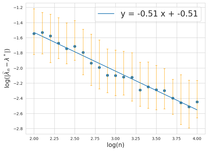
(a) *
Refer to caption

(b) Rate of μ^n\widehat{\mu}_{n}

(b) *
Refer to caption

(c) Rate of σ^n2\widehat{\sigma}^{2}_{n}

(c) *
Refer to caption
Figure 3: Case λ∗=0.5/n3/8\lambda^{*}=0.5/n^{3/8}.

(a) Rate of λ^n\widehat{\lambda}_{n}

(a) *
Refer to caption

(b) Rate of μ^n\widehat{\mu}_{n}

(b) *
Refer to caption

(c) Rate of σ^n2\widehat{\sigma}^{2}_{n}

(c) *
Refer to caption
Figure 4: Case λ∗=0.5/n1/2\lambda^{*}=0.5/n^{1/2}.

F.3 Non-distinguishable Settings

Finally, we consider the weakly identifiable and non-distinguishable setting here to demonstrate that the convergence rate for λ∗\lambda^{*} can be slower than the parametric rate when ff is near h0h_{0}. Let both h0h_{0} and ff belong to the location-scale Gaussian family. h0​(x)=f⁡(x|0,1)h_{0}(x)=f(x|0,1) and consider two cases of (λ∗,μ∗,Σ∗)(\lambda^{*},\mu^{*},\Sigma^{*}):

  1. 1.

    λ∗=0.25,μ∗=0.\lambda^{*}=0.25,\mu^{*}=0. are fixed and σ∗=1+n−1/8\sigma^{*}=1+n^{-1/8} as nn increases;

  2. 2.

    λ∗=0.25,σ∗=1.\lambda^{*}=0.25,\sigma^{*}=1. are fixed and μ∗=n−1/8\mu^{*}=n^{-1/8} as nn increases;

Recall that we have proved that {∥Δμ∗∥4+∥ΔΣ∗∥2}|λ^n−λ∗|=𝒪(n−1/2)\left\{\|\Delta\mu^{*}\|^{4}+\|\Delta\Sigma^{*}\|^{2}\right\}|\widehat{\lambda}_{n}-\lambda^{*}|=\mathcal{O}(n^{-1/2}) and λ∗(∥Δμ∗∥2+∥Δμ^n∥2+∥ΔΣ∗∥+∥ΔΣ^n∥)(∥μ^n−μ∗∥2+∥Σ^n−Σ∗∥)=𝒪(n−1/2)\lambda^{*}(\|\Delta\mu^{*}\|^{2}+\|\Delta\widehat{\mu}_{n}\|^{2}+\|\Delta\Sigma^{*}\|+\|\Delta\widehat{\Sigma}_{n}\|)(\|\widehat{\mu}_{n}-\mu^{*}\|^{2}+\|\widehat{\Sigma}_{n}-\Sigma^{*}\|)=\mathcal{O}(n^{-1/2}), where there is a mismatch in the orders of convergence rates of the location and scale parameter. Notably, the rate of convergence for λ∗\lambda^{*} also depends on the rate Δ​μ∗\Delta\mu^{*} and Δ​(σ∗)2→0\Delta(\sigma^{*})^{2}\to 0. The experiments do support this theoretical finding, where we have the rate for λ∗\lambda^{*} is ≈n−1/4\approx n^{-1/4} is the first case (as ‖Δ(σ∗)2‖2=O(n−1/4)\left\|\Delta(\sigma^{*})^{2}\right\|^{2}=O(n^{-1/4})) and it does not convergence in the second case λ∗\lambda^{*} is ≈n−1/4\approx n^{-1/4} is the first case (as ‖Δμ∗‖4=O(n−1/2)\left\|\Delta\mu^{*}\right\|^{4}=O(n^{-1/2})). The mismatch rate for ‖μ^n−μ∗‖\|\widehat{\mu}_{n}-\mu^{*}\| and ‖σ^n2−(σ∗)2‖\|\widehat{\sigma}_{n}^{2}-(\sigma^{*})^{2}\| can also be seen clearly in the second case, where the rate for the scale parameter is still of the parametric rate, whereas it is slower for the mean.

(a) Rate of λ^n\widehat{\lambda}_{n}
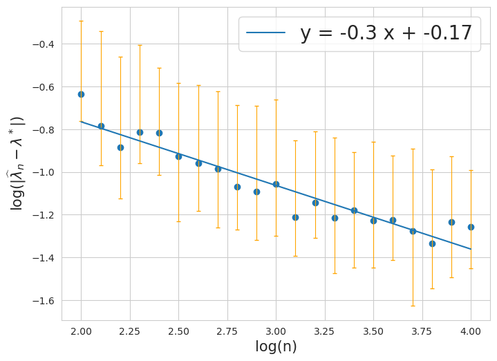
(a) *
Refer to caption

(b) Rate of μ^n\widehat{\mu}_{n}

(b) *
Refer to caption

(c) Rate of σ^n2\widehat{\sigma}^{2}_{n}

(c) *
Refer to caption
Figure 5: Case 1: μ∗=μ0\mu^{*}=\mu_{0} and (σ∗)2→σn2(\sigma^{*})^{2}\to\sigma_{n}^{2} in the rate n−1/8n^{-1/8}

(a) Rate of λ^n\widehat{\lambda}_{n}

(a) *
Refer to caption

(b) Rate of μ^n\widehat{\mu}_{n}

(b) *
Refer to caption

(c) Rate of σ^n2\widehat{\sigma}^{2}_{n}

(c) *
Refer to caption
Figure 6: Case 2: σ∗=σ0\sigma^{*}=\sigma_{0} and μ∗→μ0\mu^{*}\to\mu_{0} in the rate n−1/8n^{-1/8}.