Hydrodynamic Collapse of the Leidenfrost Vapor LayerPreprint: APS/123-QED
Abstract
During the Leidenfrost effect, a stable vapor film can separate a hot solid from an evaporating liquid. Eventually, after formation and upon cooling, the vapor layer cannot be sustained and undergoes a violent collapse evidenced by explosive boiling. Computationally, modeling this instability involves an interplay between hydrodynamics, thermodynamics, rapid evaporation, and length-scales from m to cm. Selective assumptions, made to reduce computational costs, have limited most previous studies to steady-state investigations. Here, we combine two-phase laminar flow, heat transfer, and evaporation in a finite-element simulation to examine the failure of Leidenfrost vapor layers during cooling. During periods of quiescence, the geometry of the vapor layer agrees well with steady-state lubrication theory. In the simulations, we report the local temperature of the solid at failure, , which provides a lower bound for recent experimental work using the same geometric and material conditions. Surprisingly, we find that inertial forces, which are typically ignored in theoretical treatments of the vapor layer, are responsible for initiating the instability leading to failure.
I Introduction
The Leidenfrost vapor layer was first noted by J. G. Leidenfrost in his 1756 treatise on the properties of water. He realized that water would not wet the surface of a sufficiently heated spoon and instead floated on a layer of its own vapor Leidenfrost 1756. The significance of this discovery has become important for both fundamental fluid mechanics and industrial applications Quéré 2013. Previous studies of the Leindenfrost effect have focused on the vapor layer geometry Burton et al. 2012; B. et al. 2014; Biance et al. 2003; Snoeijer et al. 6307; Duchemin et al. 2005; Lister et al. 2008; Chakraborty et al. 2022, spontaneous motion and oscillations of drops Bouillant et al. 2018; Cousins et al. 2012; Lagubeau et al. 2011; Linke et al. 2006; Gauthier et al. 2019; Ma and Burton 2018; Ma et al. 2017, drop impact on heated surfaces Tran et al. 2012; Castanet et al. 2015; Riboux and Gordillo 2016; Yao and Cai 1988; Gordillo and Riboux 2022, and “nano-painting” through particle deposition Bain 2007; Elbahri et al. 2007. The temperature at which the vapor layer forms (or fails) is important in all of these examples, yet this temperature is not well-understood. Influencing factors that determine the Leidenfrost temperature include surface roughness Kim et al. 2011; Kim et al. 2013; Kruse et al. 2013; Kim et al. 2010; Jones et al. 2019, hydrophobicity Liu and Craig 2010; Vakarelski et al. 2011; Vakarelski et al. 2012; Kim et al. 2010; Jiang et al. 2022; Bourrianne et al. 2019, solid thermal properties Freud et al. 2009; Vakarelski et al. 2011; Vakarelski et al. 2012; Yagov et al. 2015; Hsu et al. 2015; Sher et al. 2012, liquid temperature Jouhara and Axcell 2009; Freud et al. 2009; Sher et al. 2012; Yagov et al. 2015; Yagov et al. 2016; Kim et al. 2010, solid geometry Bradfield 1966; Huang and Carey 2007; Jouhara and Axcell 2009; Freud et al. 2009; Vakarelski et al. 2011; Vakarelski et al. 2012; Sher et al. 2012; Yagov et al. 2015, and liquid impurities Huang and Carey 2007; Abdalrahman et al. 2014; Hsu et al. 2015; Kim et al. 2010; Moreau et al. 2019. Most recently, studies have revealed that there are two separate Leidenfrost temperatures, a higher temperature for formation (), and a lower temperature for failure (), which are often separated by over 100∘C Harvey et al. 2021; Zhao and Patankar 2020; Chantelot and Lohse 2021a; Chantelot and Lohse 2021b.
How does a stable vapor layer fail? On smooth solid materials, is predominantly determined by van der Waals forces between the liquid and solid Zhao and Patankar 2020. Yet prior to failure, Leidenfrost vapor layers can be 10s of microns thick, suggesting that hydrodynamic stability determines . In experiments, direct measurements of the gas-fluid and gas-solid interfaces are extremely challenging. Our recent experimental work resolved microsecond dynamics of vapor layer failure using a high speed electrical technique and geometric capacitive model for the fluid interfaces Harvey et al. 2021. In the experiment, an inverse Leidenfrost system was used, which provided a well-defined vapor layer surface area despite evaporation. The hot solid material was a metallic rod with a spherical tip of radius, = 8 mm (Fig. 1a), immersed in a bath of salt water of height above the tip. After formation of the vapor layer at high temperatures, the solid was cooled until the vapor layer collapsed and explosive boiling ensued. We found a consistent failure temperature, C (Fig. 1b), for all experiments of various metals and salt concentrations. This suggests that a hydrodynamic instability, i.e. surface waves growing in amplitude, incited vapor layer collapse Harvey et al. 2021. This can be seen in Fig. 1c-d and Movie S1. Beyond these experimental results, computational fluid mechanics can be used to specify the dominant hydrodynamic mechanism that initiates vapor layer collapse.

Previous simulations Snoeijer et al. 6307; B. et al. 2014; van Limbeek et al. 2017; Chakraborty et al. 2022 have succeeded in matching the experimentally-measured geometries of steady-state Leidenfrost drops Biance et al. 2003; Burton et al. 2012; van Limbeek et al. 2017. However, vapor layer failure is inherently dynamic, and steady-state approximations are invalid in this regime. Additionally, other simplifying assumptions commonly used to describe the fluid mechanics of vapor layers may be invalid near failure. First, lubrication theory is typically used to describe the vapor layer, which assumes the thickness (10-100 m) is slowly-varying in space and completely ignores inertia B. et al. 2014; Chakraborty et al. 2022. The latter is especially important since the Reynolds number in the vapor layer can be of order unity Ma and Burton 2018. Second, nearly all theory and computational work assumes a uniform temperature throughout the fluid, with few exceptions van Limbeek et al. 2017. A uniform temperature neglects convection, heat transfer, and phase change through evaporation Chakraborty et al. 2022. These simplifying assumptions significantly reduce the computational costs of modeling vapor layers between solids and liquids. In some cases, different regimes of stability can be found between steady-state solutions Duchemin et al. 2005; Lister et al. 2008; Snoeijer et al. 6307. However, they provide little insight into the rapid dynamics of vapor layer failure.
Here, we use a COMSOL Multiphysics simulation to combine two-phase laminar flow, heat transfer, and evaporation to investigate the dynamics and failure of Leidenfrost vapor layers upon cooling. The axisymmetric model uses the same inverted Leidenfrost geometry as the experiments, and is validated by matching quiescent interface profiles prior to failure with a steady-state lubrication model, similar to previous studies. Upon cooling, we find that the vapor layer undergoes a rapid and violent failure, similar to experiments. By modeling a wide range of solid material geometries and thermal properties, we demonstrate that the temperature at failure, , agrees well with previous experiments, and in fact provides a lower bound on for smooth surfaces. Failure occurs by means of a series of growing sinusoidal perturbations in the liquid-vapor interface that approach the surface. The leading perturbation that touches the surfaces first causes failure at a single point. By varying the surface tension and molecular weight of the gas in the simulation, we found that the inertia of the evaporated gas, almost always neglected in theory, is paramount to inciting the instability which ultimately results in vapor layer collapse.
II COMSOL Simulation Details
We simulated a three dimensional (3D), axisymmetric inverse Leidenfrost system consisting of a hot object immersed in a heated liquid bath. We used a cylindrical coordinate system with radial coordinate and axial coordinate . The simulation space was a 40 mm 40 mm box consisting of a solid rod with a spherical tip of radius centered on the axis of symmetry, = 0 mm, Fig. 2a. The bottom tip of the hot solid was fixed at = 22 mm and the initial liquid height was = 21 mm. During the simulation, the height of the liquid was slowly raised until it reached a final height , forming a vapor layer around the spherical tip. This process is shown in Movie S2. The surface area of the vapor layer was controlled by varying the radius of the spherical tip, 2 mm mm, and the liquid level 0.5 mm mm, Fig. 1a. To suppress superheating of the liquid and minimize wall boundary effects, the outer boundary at = 40 mm was held at 70 ∘C with a slip condition (no restrictions on tangential velocity).

In the fluid domain we modeled a two-phase incompressible fluid with gravity using the non-conservative phase field equations. The non-conservative form must be used to avoid excessive convergence times while maintaining accurate results for our simulations Sun and Beckermanm 2007; Chiu and Lin 2011. The fluid domain mesh size was adaptive, ranging from 2.25 m - 195 m. In the solid domain we found a mesh size of 3 m - 800 m led to reproducible results. Within COMSOL, the laminar flow and two-phase flow modules allow for gradients in density and viscosity, thus the Navier-Stokes equations are defined as follows with the corresponding incompressibility condition COMSOL Multiphysics®, v. 5.3. COMSOL AB 2020:
| (1) | |||
| (2) |
Here is the velocity, is the acceleration due to gravity, is the density of the fluid, is the pressure, and is the dynamic viscosity of the fluid.
We note that previous studies investigating steady-state solutions of the vapor layer only consider the fluid dynamics of the vapor flow using a lubrication approximation Snoeijer et al. 6307; B. et al. 2014. The lubrication approximation neglects the inertial terms of the Navier-Stokes equations and instead assumes Stokes flow,
| (3) |
in the vapor layer, which is typically only 10 m - 100 m thick and varies slowly along the solid surface. The evaporating liquid is considered a solid boundary with no-slip, or is modeled as a Navier-Stokes fluid B. et al. 2014; Chakraborty et al. 2022 where evaporation is parameterized and constant along the interface. We will use this same approximation in Sec. III to verify our full simulation results well before vapor layer failure.
Evaporation was added to the COMSOL model as a heat source term, , defined in the literature as Jafari and Okutucu-Özyurt 2015; Research and Consulting 2018:
| (4) |
where is the latent heat of vaporization of the liquid defined in Table 1. The rate of mass vaporization, , and the interface delta function, , are defined as:
| (5) |
and
| (6) |
Here , , and are defined in Table 1, m/s is a tuning parameter, is a small mathematical number to ensure there are no divisions by 0 when using Jafari and Okutucu-Özyurt 2015, is the temperature of the fluid, and is the volume fraction of water. In this formulation, the phase field takes values from -1 (liquid) to 1 (vapor). The same equations for and are used by Jafari et al. to successfully simulate a growing vapor bubble in a confined tube Jafari and Okutucu-Özyurt 2015.
| Parameter | Expression | units | Description |
|---|---|---|---|
| 0.018 | kg/mol | molecular weight of water | |
| 42000/ | J/kg | latent heat of vaporization | |
| 373 | K | saturation temperature | |
| 1000 | kg/m3 | density of water | |
| ()/(8.314+eps)) | kg/m3 | density of water vapor | |
| 0.001 | m/s | tuning parameter | |
| 195 | m | maximum grid size | |
| 101325 | Pa | atmospheric pressure | |
| Pa s | dynamic viscosity of the fluid | ||
| Pa s | dynamic viscosity of the gas | ||
| 0.0588 | N/m | surface tension coefficient | |
| 0.63 | W/(mK) | thermal conductivity of water | |
| T | W/(mK) | thermal conductivity of vapor | |
| W/(mK) | thermal conductivity for two-phase flow | ||
| 4200 | J/(kgK) | specific heat of liquid water | |
| 1840 | J/(kgK) | specific heat of water vapor | |
| J/(kgK) | specific heat for two-phase flow |
A weak expression, , in the fluid domain helps produce smooth results. = test() +test() , where test() is a localized sampling function, is the source term of the phase field equation, is the source term in the continuity equation, and is the volume fraction of the vapor. The phase field help variable is
| (7) |
where is the interfacial thickness variable and . The help variable describes the interfacial free energy between the two phases Patel et al. 2019; Jafari and Okutucu-Özyurt 2015. All other variables are defined in Table 1.
For all simulations, we assume properties of the liquid and vapor phase associated with liquid and gaseous water. However, we used a larger value for the viscosity of the water vapor since it was necessary for numerical stability (as discussed in Sec. IV). A typical initial phase field frame is shown in Fig. 2a. For each simulation, initialization included defining the thermal properties of the hot solids, Table 2, and the starting isothermal temperature of all phases. For most cases, 650 K was used as the starting solid temperature. For some simulations, an increased solid temperature was required for large values of and low thermal conductivity materials. The initial water and vapor temperatures were set to 90∘C and 110∘C, respectively.
| Material | ||||
|---|---|---|---|---|
| Copper | Cu | 386 | 8940 | 385 |
| Aluminum | Al | 247 | 2710 | 897 |
| Iron | Fe | 60 | 7800 | 449 |
| Titanium | Ti | 7 | 4420 | 540 |
| Glass | 0.8 | 2500 | 792 |
An atmospheric pressure outlet at = 40 mm allowed gas to escape, while an inlet at = 0 mm had a variable pressure, , which controlled the equilibrium water level . Initially, was defined and maintained for 1 s at , where = 21 mm. After 1 s of simulation time, the pressure was slowly increased according to , which raised the water height until + 1 mm), as shown in Fig. 2b. As the water level rose a vapor layer spontaneously formed around the hot object due to evaporation. The pressure boundary at mm conveniently minimized the effects of using the non-conservative mass equations by maintaining with as much water inflow as was necessary. Once the desired was achieved, the simulations continued unhindered until the vapor layer failed. Time series for typical simulations of copper, aluminum, and titanium solid objects with mm and mm, are shown in Figs. 3-5, respectively. These simulations will be discussed further in Sec. IV.


III Lubrication Model and Comparison
To help ensure the validity of the COMSOL Multiphysics simulations, we compared quiescent, near steady-state profiles at early times with a steady-state lubrication approximation. Nearly identical lubrication models have been used to describe the air or evaporated vapor flow under a levitated drop Lister et al. 2008; Snoeijer et al. 6307; Duchemin et al. 2005; Chakraborty et al. 2022; Sobac et al. 2017; B. et al. 2014. In particular, predictions from Snoeijer et al. Snoeijer et al. 6307 show excellent agreement with experiments of Leidenfrost drops Burton et al. 2012; Biance et al. 2003. The lubrication approximation balances the leading order pressure gradient terms driving the tangential flow in the vapor layer with gradients in viscous stress, and ensures conservation of mass in the flow. For the lubrication model presented here, both the liquid-vapor interface and the solid material are considered motionless. This is valid if the viscosity of the liquid is considerably larger than the vapor. Although in our COMSOL simulation the liquid is only twice as viscous as the vapor (Table 1), this simplification allows one to ignore flow in the liquid phase and serves as a leading-order description of the physics.
In general, the lubrication approximation makes two major assumptions to simplify the governing equations. First, , where is the local gap thickness and is the total vapor path length. This is valid in steady-state Leidenfrost drops where m and cm. Second, the vapor has a parabolic velocity profile within the gap such that , and is the mean velocity in the tangential direction Lautrup 2004. A schematic of this geometry is shown in Fig. 6a. A further simplification is typically made by assuming steady-state, so that . Although this results in a system of 2 ODEs for and , during failure of the vapor layer these assumptions break down. The wavelength and amplitude of the instability, which causes vapor layer failure, grow in time so that , Fig. 6b. The wavelength becomes the important longitudinal length scale, , thus breaking the assumption that . Subsequently, we only can compare our simulations to the lubrication approximation at steady-state times well before failure.
In our lubrication model, we ignore inertia. Estimates for the flow beneath centimeter-scale droplets suggest that Re 0.3 Ma et al. 2017, so this assumption is reasonable. Since we are not explicitly considering evaporation, we assume that there is a constant flow of gas that feeds the vapor layer at velocity . We only consider the flow around the lower part of a hemisphere immersed in the liquid, and use axisymmetric spherical coordinates so that the tip of the hemisphere (with radius ) corresponds to (Fig. 1a). Both the film thickness, , and the depth-averaged velocity, , vary with the angular coordinate. We will assume that , and that , where prime denotes differentiation with respect to . This means that the film is thin and that its thickness varies slowly along the edge of the hemisphere, an assumption that must break down at failure.
With these assumptions, there are two differential equations that describe the steady state profiles of and :
| (8) | |||
| (9) |
Equation 8 comes from mass conservation of the gas in the vapor layer, assuming that from symmetry considerations. Equation 9 balances the pressure gradient necessary to drive the flow in the lubricating vapor layer with the pressure gradient determined by hydrostatic (gravitational) forces and variations in the Laplace pressure. The variable is the total curvature of the interface, and can be calculated by taking the divergence of the normal vector to the liquid-vapor interface:
| (10) | |||
| (11) |
where the spherical coordinate is evaluated at after differentiation. Here we have kept the full curvature with no approximations in order to correctly model the shape of the interface all the way to the boundary.
Equation 8 can be solved directly for and inserted into Eq. 9, resulting in a third-order differential equation for . For a given gas input velocity (), we chose initial values of and since = 0 by axisymmetry. We then solved the resulting equation for until we matched the height of the liquid level at the outer boundary (), and required that , so that the normal to the interface pointed in the -direction. Importantly, we emphasize that these are steady solutions, so there are no dynamics. This means that for a given and set of boundary conditions, a solution may not exist. In fact, the structure of the branches where solutions exist is quite complicated, as may be expected from similar problems considering the lubricating flow under droplets Lister et al. 2008; Duchemin et al. 2005. In reality, a vapor layer may exist for all thicknesses and boundary conditions, but will fluctuate in time. Periods of quiescent behavior in the experiments Harvey et al. 2021 and COMSOL simulations may correspond to regimes where steady solutions of the lubricating vapor layer exist.
Using the properties for water and vapor given in Table 1, we show comparisons between the lubrication model and COMSOL simulation at early times in Fig. 7. The lubrication model parameters , , and were adjusted to best match the COMSOL profiles where the phase field (50% vapor, 50% liquid). The agreement is excellent for different values of the external water level . However, the lubrication model tends to have a minimum in that is smaller than in the COMSOL simulation, meaning that the interface comes closer to the solid boundary. This may be due to the variation in evaporation rate in the COMSOL model, which is determined by thermodynamics, whereas the lubrication model assumes a constant value of along the entire interface. Figure 8 shows the solutions for and that correspond to the profile shown in Fig. 7b. The minimum in aligns with the maximum in the velocity . The near linear increase in the velocity from is a result of the increasing mass flux into the vapor layer (Eq. 8). The peak in 0.5 m/s agrees very well with the velocity from the full COMSOL simulation, discussed in more detail in Sec. IV.
IV Failure of the Vapor Layer


The primary purpose of the COMSOL simulations was to provide a quantitative understanding of the failure of Leidenfrost vapor layers. As such, we varied the geometry of the vapor layer and the thermal properties of the hot solid to best match our previous experimental results Harvey et al. 2021. In experiments, we found the minimum Leidenfrost Temperature, = 140∘C, was independent of solid thermal properties, geometry, and salt concentration of the liquid. However, the physical geometry of the metallic hot solid was limited by experimental constraints. Here, we show how our simulations can replicate experimental results, explore a larger variation of system parameters, and provide insight into the instability that drives vapor layer failure.
A typical simulation evolved as described in Sec. II until vapor layer failure (explosive collapse). As the water level rose, evaporation produced a vapor layer of order 100-200 m around the hot solid object. During subsequent cooling, for solids such as aluminum or copper with high thermal conductivity, the solid was nearly isothermal during the simulation (Figs. 3 & 4). However, there was significant local cooling near the tip of the solid in materials with low thermal conductivity, such as titanium (Fig. 5). In all simulations, local cooling of the liquid due to evaporation, determined by , was initially strong enough to create a downward convective flow, as illustrated in Figs. 3-5. This downward flow eventually subsided as the solid cooled, but persisted until failure for titanium. As a consequence, the flow in the liquid adjacent to the vapor layer could reverse direction during the simulation.
Upon further cooling of the solid, the vapor layer thinned and developed time-dependent variations in thickness; a dynamic instability leading to failure. In experiments, this instability manifested as visible surface waves, Fig. 1c, which proceeded the explosive collapse of the vapor layer. In simulations, the instability appeared as the same interfacial wave, sometimes many waves, which grew and moved along the surface until fluid-solid contact (last frames of Figs. 3-5). This is most clearly illustrated in Fig. 9 (Movie S3), which shows a times series of vapor layer failure for a copper object. The location of the failure point was somewhat stochastic and typically did not occur at the minimum in (e.g., Fig. 8a).
Figure 10 shows an unwrapped angular plot of both the phase field and velocity magnitude from the same simulation. An obvious feature seen here is the appearance of local liquid contact at the tip, . This occurred in nearly all simulations, but most prominently for solids with lower thermal conductivity and small values of . This apparent contact did not produce explosive boiling, and the vapor layer failure seemed to occur at smaller values of away from the tip. Additionally, this apparent contact was not observed in experiments Harvey et al. 2021, and is likely a consequence of the finite thickness of our phase field or the enforced axisymmetric geometry. Nevertheless, at the failure point away from the tip, liquid-solid contact occurred in 10s of milliseconds, which agrees well with the rapid timescales for collapse measured in experiments Harvey et al. 2021. At the contact point, the temperature of the solid, , was still well above the boiling point of water, so rapid evaporation ensued at the moment of contact. Subsequently, the COMSOL simulation often crashed due to the explosive nature of the event and the inability to capture such rapid dynamics. However, we can analyze the results of the simulation leading to failure and compare directly to experiments.
In our experimental work, we could precisely determine the failure of the vapor layer in time as a discontinuity in the thickness measurement Harvey et al. 2021. That discontinuity correlated to the wetting of the surface as liquid came into contact with the hot solid. To directly compare simulations and experiments we define vapor layer failure as the initial contact point between the fluid and solid. Therefore, was measured locally in the solid at the contact point one time-step before collapse. Furthermore, to compare among simulations and experiments with different values of the tip radius and water height, , we computed the effective surface area of the vapor layers, . Here is the surface area of the vapor layer found by integrating over a semi-sphere Boas 2005:
| (12) |
Here is the height above the tip measured at the inflection point of the contour (Fig. 11a). We divide by to normalize the area, where mm is the capillary length of boiling water. Using two parameters, the radius of the hot solid, 2 mm, and the water height, mm, an effective area range of was achieved in simulations. In Fig. 11b we plot as a function of for hot objects of various radii and thermal properties. The thermal properties correlated to real material values described in Table 2.
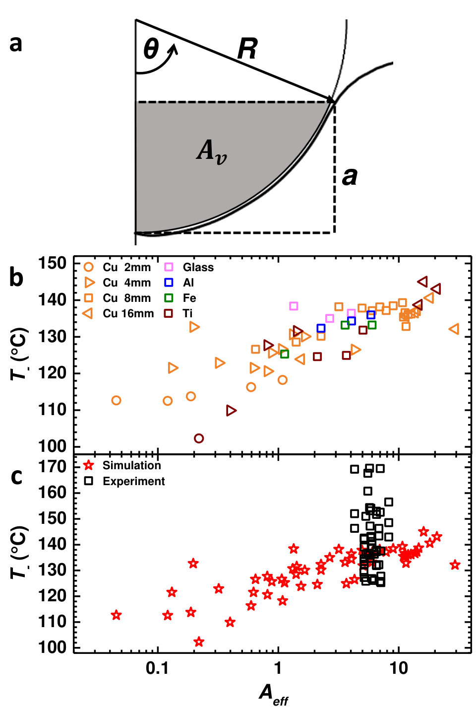

Just as in experiments (Fig. 1b), we found that was nearly independent of the thermal properties of the solid. Generally, decreased as decreased and even approached the boiling temperature Baumeister et al. 1966; Harvey et al. 2021; Zaitsev et al. 2017, yet appeared to plateau at larger values of . The plateau region begins at , so that the characteristic size of the vapor layer is approximately the capillary length, . This is consistent with experiments with liquid drops where the effective area could be easily varied by more than 1 decade Harvey et al. 2021. In the experiments using an hot object immersed in a bath, as simulated here, the effective area was limited to a much smaller range, as shown in Fig. 1b. In this range of , the simulations act as a lower bound for experimental values of . This should be expected since there were uncontrollable factors in the experiments such as microscopic debris in the water and finite surface roughness of the hot solid. Both of these effects could lead to premature failure at higher temperatures. Overall, it is remarkable that the simulations agree quantitatively with the experiments despite their simplifications, such as enforcing an axisymmetric geometry, and necessitating a higher vapor viscosity for numerical stability. This implies that the nature of the failure mechanism depends on other fluid properties of the vapor.
To better understand the evolution of failure, we investigated larger solid objects ( mm) where multiple perturbations could grow, move, and evolve prior to failure. Figure 12a-b shows two final frames from the simulation. A relatively smooth vapor layer quickly developed a series of thickness and velocity perturbations resembling a wave train. The spacing between the perturbations decreased as decreased towards the vapor exit. Since the average vapor velocity also increases near the exit (i.e., Fig. 8b), we surmise that the local growth of each perturbation depends on the local vapor velocity. To visualize this more clearly, we plot the unwrapped phase contour and velocity magnitude in Fig. 12c-d. Prior to the growth of the perturbations, the thickness profile agrees well with the prediction from the lubrication model, Fig. 8a. Just before failure, there is a clear characteristic wavelength () for the series of perturbations that develop. In units of length, this wavelength corresponds to mm. The appearance of a definitive wavelength suggests a hydrodynamic instability is initiated that leads to liquid-solid contact.
How does this hydrodynamic instability determine the failure temperature? In the vapor layer flow, there are two major forces that could naturally lead to an instability. First, the pressure in the vapor layer acts against buoyancy, so that a Rayleigh-Taylor (RT) type of instability could lead to liquid touching the surface. In fact, the RT instability is known to determine the maximum size of Leidenfrost drops Biance et al. 2003; Burton et al. 2012; Snoeijer et al. 6307. Second, the rapid flow in the vapor layer applies a stress to the liquid-vapor interface and can lead to a Kelvin-Helmholtz type of instability. However, the simplest example of both of these instabilities lead to critical wavelengths of order 1-2 cm Lautrup 2004, not millimeters, as we observe in our simulations and experiments Harvey et al. 2021. In the Leidenfrost vapor layer, there are additional complexities that need to be considered, such as the presence of a solid surface, viscous and inertial forces, evaporation, and a non-planar geometry.
Consider the simple picture of a wave at the gas-fluid interface depicted in Fig. 6b and the forces acting on it. Surface tension and evaporation both act as restoring forces to suppress the growth of liquid-vapor interface perturbations. For example, the rate of evaporation should increases as the liquid approaches the solid, producing a higher local pressure. As mentioned, buoyant forces (gravity) can instigate the growth of perturbations (RT instability), but only for centimeter-scale wavelengths. The net effect of viscous lubrication pressure depends on the geometry of the perturbation. For a symmetric perturbation, a high and low pressure develop that are equal in magnitude on each side of the perturbation, resulting in no net lift. Thus, for an infinitesimal sinusoidal perturbation to a flat vapor interface, viscous forces alone may not explain this instability.
We hypothesize that inertial forces in the vapor layer can lead to a reduction in pressure sufficient to draw the liquid-vapor interface close to the solid, initiating contact and failure. Indeed, inertia has been shown to be necessary in the formation of finite-time singularities in similar two-dimensional flows Dupont et al. 1993; Burton and Taborek 2007. An overly simplistic balance of Laplace and Bernoulli pressure can illustrate this idea. Referring to Fig. 6 again, consider a sinusoidal perturbation of amplitude and wavelength to the flat liquid-vapor interface,
| (13) |
where is the mean vapor layer thickness. Conservation of mass in the vapor layer leads to an increase in the velocity, , where the perturbation is closest to the surface,
| (14) |
where is the mean velocity in the vapor layer. The reduction in pressure due to Bernoulli suction is given by:
| (15) |
The change in Laplace pressure from the curvature of the interface is given by:
| (16) |
where the derivative is evaluated at point of closest approach. If , the perturbation will grow. Combining these equations and assuming , we can derive an expression for the critical wavelength that satisfies this condition:
| (17) |
To estimate , we use the contour line (i.e., Fig. 12c) where m, m/s, N/m, and the density 300-500 kg/m3 since we do not have a sharp liquid-vapor interface (Fig. 10a). With these numerical values, 2.8-3.6 mm, which is in reasonable agreement with the wavelengths observed in Fig. 12b. In experiments, the liquid-vapor phase separation is much sharper and well-defined. As a consequence, to estimate , one must use the density of water vapor near boiling, kg/m3. Additionally, at failure, the average thickness of the vapor layer is 15 m Harvey et al. 2021. The velocity in experiments should be much larger than the simulations because is smaller, leading to enhanced heat transfer and a higher rate of evaporation, and by conservation of mass (Eq. 8). With this in mind, a mean velocity of m/s results in 2.5 mm. It is worth noting that dynamic capillary waves with wavelength 2-3 mm were observed in the experiments Harvey et al. 2021. Thus, it is possible that failure may occur by the cooling and thinning of the vapor layer until naturally-excited waves can be suctioned to the surface by Bernoulli pressure in the vapor layer.
There are 2 independent parameters in Eq. 17 that we can vary in our simulations: and . Naively, one would expect that increasing would lead to lower values of due to its stabilizing influence against perturbations. Additionally, increasing would enhance the Bernoulli suction and lead to larger values of . However, Fig. 13a shows that increasing leads to larger values of . An important consequence of increasing the surface tension is that the liquid-vapor interface profile varies with . Also, the capillary length increases with , so that a smaller vapor layer area has to support the hydrostatic pressure of a larger surface depression. Thus, a higher temperature is required to generate enough evaporative flow to balance this pressure. Such a large increase in from evaporation may actually enhance the Bernoulli effect in Eq. 17.

A more direct test of Eq. 17 can be achieved by simply changing the molecular weight of the vapor, . The temperature-dependent vapor density, , is proportional to , as seen in Table 1. Since variations in do not affect the surface tension or viscosity, for example, the lubrication approximation that determines the steady-state interface profile is unchanged. This is what we observe, as illustrated in Fig. 13b-d. Increasing leads to larger values of , while the interface profile and geometry remain essentially unchanged. Examining Eq. 17, increases in () would lead to smaller values of the critical wavelength, meaning that the interface is less stable to perturbations, and will fail at higher temperatures. Figure 14 shows how varying or monotonically affects , from 120∘C-260∘C. In our simulations, we note that strictly changing will also change the latent heat , as given in Table 1. For completeness, we ran two sets of simulations, ones where we held fixed at J/kg, and ones where was allowed to vary with . Both sets showed nearly identical results for , indicating that hydrodynamic inertial effects () played a dominant role in determining and the failure of the vapor layer.
V Conclusion
Using simulations that combine two-phase laminar flow, heat transfer, and evaporation, we examined the formation and ultimate failure of Leidenfrost vapor layers around smooth objects. Our simulations were verified by comparing steady-state vapor layer profiles to a viscous lubrication approximation, showing excellent agreement. The failure of the vapor layer is highly dynamic and involves many thermo-physical effects not present in lubrication theory, which is often used to describe Leidenfrost vapor layers. Our results here strongly support recent experimental observations Harvey et al. 2021: 1) is nearly independent of the thermal properties of the solid material, 2) can approach boiling temperatures for small vapor layer surface areas, and plateaus for areas larger than the capillary length of the liquid, and 3) A hydrodynamic instability determines and the mechanism of vapor layer failure. In the simulations, liquid-solid contact and explosive boiling occurs at a single point determined by the rapid growth of well-defined perturbations in a few milliseconds. A major finding of this work is that gas inertia, which is often completely ignored in theories of Leidenfrost vapor layers, dominates the instability leading to failure. The local reduction in pressure near a surface perturbation draws the liquid-vapor interface to the surface. These results demonstrate that the short time scales inherent in Leidenfrost vapor layers can be successfully captured in multiphysics simulations, opening new paths to study dynamic Leidenfrost phenomena. In future studies, we suggest that controllable variations in surface geometry or roughness may be harnessed to increase or decrease , in a similar way to the formation temperature of Leidenfrost vapor layers Jiang et al. 2022.
Acknowledgements.
We gratefully acknowledge conversations with Eric Weeks. This work was supported by the NSF DMR Grant No. 2010524.References
- Leidenfrost (1756) J. G. Leidenfrost, De aquae communis nonnullis qualitatibus tractatus (Ovenius, 1756).
- Quéré (2013) D. Quéré, Leidenfrost dynamics, Annu. Rev. Fluid Mech. 45, 197 (2013).
- Burton et al. (2012) J. C. Burton, A. L. Sharpe, R. C. A. van der Veen, A. Franco, and S. R. Nagel, Geometry of the vapor layer under a leidenfrost drop, Phys. Rev. Lett. 109, 074301 (2012).
- B. et al. (2014) S. B., A. Rednikov, S. Dorbolo, and P. Colinet, Leidenfrost effect: Accurate drop shape modeling and refined scaling laws, Phys. Rev. E 90, 053011 (2014).
- Biance et al. (2003) A.-L. Biance, C. Clanet, and D. Quéré, Leidenfrost drops, Phys. Fluids 15, 1632 (2003).
- Snoeijer et al. (6307) J. H. Snoeijer, P. Brunet, and J. Eggers, Maximum size of drops levitated by an air cushion, Phys. Rev. E 79, 053011 (036307).
- Duchemin et al. (2005) L. Duchemin, J. R. Lister, and U. Lange, Static shapes of levitated viscous drops, J. Fluid Mech. 533, 161 (2005).
- Lister et al. (2008) J. R. Lister, A. B. Thompson, A. Perriot, and L. Duchemin, Shape and stability of axisymmetric levitated viscous drops, J. Fluid Mech. 617, 167 (2008).
- Chakraborty et al. (2022) I. Chakraborty, M. V. Chubynsky, and J. E. Sprittles, Computational modelling of leidendfrost drops, Journal of Fluid Mechanics 936, https://doi.org/10.1017/jfm.2022.66 (2022).
- Bouillant et al. (2018) A. Bouillant, T. Mouterde, P. Bourrianne, A. Lagarde, C. Clanet, and D. Queéré, Leidenfrost wheels, Nature Physics (2018).
- Cousins et al. (2012) T. R. Cousins, R. E. Goldstein, J. W. Jaworski, and A. I. Pesci, A ratchet trap for Leidenfrost drops, J. Fluid Mech. 696, 215 (2012).
- Lagubeau et al. (2011) G. Lagubeau, M. Le Merrer, C. Clanet, and D. Quéré, Leidenfrost on a ratchet, Nature Phys. 7, 395 (2011).
- Linke et al. (2006) H. Linke, B. J. Alemán, L. D. Melling, M. J. Taormina, M. J. Francis, C. C. Dow-Hygelund, V. Narayanan, R. P. Taylor, and A. Stout, Self-propelled Leidenfrost droplets, Phys. Rev. Lett. 96, 154502 (2006).
- Gauthier et al. (2019) A. Gauthier, C. Diddens, R. Proville, D. Lohse, and D. van der Meer, Self-propulsion of inverse leidenfrost drops on a cryogenic bath, Proc. Natl. Acad. Sci. USA 116, 1174 (2019).
- Ma and Burton (2018) X. Ma and J. C. Burton, Self-organized oscillations of leidenfrost drops, Journal of Fluid Mechanics 846, 263 (2018).
- Ma et al. (2017) X. Ma, J. Liétor-Santos, and J. C. Burton, Star-shaped oscillations of leidenfrost drops, Physical Review Fluids 2, 031602(R) (2017).
- Tran et al. (2012) T. Tran, H. J. J. Staat, A. Prosperetti, C. Sun, and D. Lohse, Drop impact on superheated surfaces, Phys. Rev. Lett. 108, 036101 (2012).
- Castanet et al. (2015) G. Castanet, O. Caballina, and F. Lemoine, Drop spreading at the impact in the leidenfrost boiling, Phys. Fluids 27, 063302 (2015).
- Riboux and Gordillo (2016) G. Riboux and J. M. Gordillo, Maximum drop radius and critical weber number for splashing in the dynamical leidenfrost regime, J. Fluid Mech. 803, 516–527 (2016).
- Yao and Cai (1988) S.-C. Yao and K. Y. Cai, The dynamics and leidenfrost temperature of drops impacting on a hot surface at small angles, Exp. Therm. and Fluid Sci. 1, 363 (1988).
- Gordillo and Riboux (2022) J. M. Gordillo and G. Riboux, The initial impact of drops cushioned by an air or vapour layer with applications to the dynamic leidenfrost regime, Journal of Fluid Mechanics 941 (2022).
- Bain (2007) C. Bain, Drip painting on a hot canvas, Nature Nanotechnology 2, 344 (2007).
- Elbahri et al. (2007) M. Elbahri, D. Paretkar, K. Hirmas, S. Jebril, and R. Adelung, Anti-lotus effect for nanostructuring at the leidenfrost temperature, Advanced Materials 19, 1262 (2007).
- Kim et al. (2011) H. Kim, B. Truong, J. Buongiorno, and L.-W. Hu, On the effect of surface roughness height, wettability, and nanoporosity on leidenfrost phenomena, Appl. Phys. Lett. 98, 083121 (2011).
- Kim et al. (2013) S. H. Kim, H. S. Ahn, J. Kim, M. Kaviany, and M. H. Kim, Dynamics of water droplet on a heated nanotubes surface, Appl. Phys. Lett. 102, 233901 (2013).
- Kruse et al. (2013) C. Kruse, T. Anderson, C. Wilson, C. Zuhlke, D. Alexander, G. Gogos, and S. Ndao, Extraordinary shifts of the leidenfrost temperature from multiscale micro/nanostructured surfaces, Langmuir 29, 9798 (2013).
- Kim et al. (2010) H. Kim, J. Buongiorno, L. Hu, and T. Mckrell, Nanoparticle deposition effects on the minimum heat flux point and quench front speed during quenching in water-based alumina nanofluids, International Journal of Heat and Mass Transfer 53, 1542 (2010).
- Jones et al. (2019) P. R. Jones, C. Chuang, T. Sun, T. Y. Zhao, K. Fezzaa, J. C. Takase, D. Singh, and N. A. Patankar, High-speed x-ray imaging of the leidenfrost collapse, Scientific Reports 9, 1598 (2019).
- Liu and Craig (2010) G. Liu and V. S. J. Craig, Macroscopically flat and smooth superhydrophobic surfaces: Heating induced wetting transitions up to the leidenfrost temperature, Faraday Discussions 146, 141 (2010).
- Vakarelski et al. (2011) I. U. Vakarelski, J. O. Marston, D. Y. C. Chan, and S. T. Thoroddsen, Drag reduction by leidenfrost vapor layers, PRL 106, 214501 (2011).
- Vakarelski et al. (2012) I. Vakarelski, N. A. Patankar, J. O. Marston, D. Y. C. Chan, and S. T. Thoroddsen, Stabilization of liedenfrost vapour layer by textured superhydrophobic surfaces, Nature 489, 274 (2012).
- Jiang et al. (2022) M. Jiang, Y. Wang, F. Liu, H. Du, Y. Li, H. Zhang, S. To, S. Wang, C. Pan, J. Yu, et al., Inhibiting the leidenfrost effect above 1,000° c for sustained thermal cooling, Nature 601, 568 (2022).
- Bourrianne et al. (2019) P. Bourrianne, C. Lv, and D. Quéré, The cold leidenfrost regime, Science advances 5, eaaw0304 (2019).
- Freud et al. (2009) R. Freud, R. Harari, and E. Sher, Collapsing criteria for vapor film around solid spheres as a fundamental stage leading to vapor explosion, Nuclear Engineering and Design 239, 722 (2009).
- Yagov et al. (2015) V. V. Yagov, A. R. Zabirov, and M. A. Lexin, Unsteady heat transfer during subcooled film boiling, Heat and Mass Transfer and Properties of Working Fluids and Materials 62, 833 (2015).
- Hsu et al. (2015) S. Hsu, Y. Ho, M. Ho, J. Wang, and C. Pan, On the formation of vapor film during quenching in de-ionized water and elimination of film boiling during quenching in natural sea water, International Journal of Heat and Mass Transfer 86, 65 (2015).
- Sher et al. (2012) I. Sher, R. Harari, R. Reshef, and E. Sher, Film boiling collapse in solid spheres immersed in a sub-cooled liquid, Applied Thermal Engineering 36, 219 (2012).
- Jouhara and Axcell (2009) H. Jouhara and B. P. Axcell, Film boiling heat transfer and vapour film collapse on spheres, cylinders, and plane surfaces, Nuclear Engineering and Design 239, 1885 (2009).
- Yagov et al. (2016) V. V. Yagov, M. A. Lexin, A. R. Zabirov, and O. N. Kaban’kov, Film boiling of subcooled liquids. part i: Leidenfrost phenomenon and experimental results for subcooled water, International Journal of Heat and Mass Transfer 100, 908 (2016).
- Bradfield (1966) W. S. Bradfield, Liquid-solid contact in stable film boiling, Ind. Eng. Chem. Fundamen. 5, 200 (1966).
- Huang and Carey (2007) C.-K. Huang and V. P. Carey, The effects of dissolved salt on the leidenfrost transition, International Journal of Heat and Mass Transfer 50, 269 (2007).
- Abdalrahman et al. (2014) K. H. M. Abdalrahman, Sabariman, and E. Specht, Influence of salt mixture on the heat transfer during spray cooling of hot metals, International Journal of Heat and Mass Transfer 78, 76 (2014).
- Moreau et al. (2019) F. Moreau, P. Colinet, and S. Dorbolo, Explosive leidenfrost droplets, Physical Review Fluids 4, 013602 (2019).
- Harvey et al. (2021) D. Harvey, J. Méndez Harper, and J. C. Burton, Minimum leidenfrost temperature on smooth surfaces, Phys. Rev. Lett. 127, 104501 (2021).
- Zhao and Patankar (2020) T. Y. Zhao and N. A. Patankar, The thermo-wetting instability driving leidenfrost film collapse, PNAS 117, 13321 (2020).
- Chantelot and Lohse (2021a) P. Chantelot and D. Lohse, Leidenfrost effect as a directed percolation phase transition, Physical review letters 127, 124502 (2021a).
- Chantelot and Lohse (2021b) P. Chantelot and D. Lohse, Drop impact on superheated surfaces: short-time dynamics and transition to contact, Journal of fluid mechanics 928 (2021b).
- van Limbeek et al. (2017) M. A. J. van Limbeek, M. H. Klein Schaarsberg, B. Sobac, A. Rednikov, C. Sun, P. Colinet, and D. Lohse, Leidenfrost drops cooling surfaces: theory and interferometric measurement, J. Fluid Mech. 827, 614 (2017).
- Sun and Beckermanm (2007) Y. Sun and C. Beckermanm, Sharp interface tracking using the phase-field equation, Journal of Computational Physics 220, 626 (2007).
- Chiu and Lin (2011) P.-H. Chiu and Y.-T. Lin, A conservative phase field method for solving incompressible two-phase flows, Journal of Computational Physics 230, 185 (2011).
- COMSOL Multiphysics®, v. 5.3. COMSOL AB (2020) COMSOL Multiphysics®, v. 5.3. COMSOL AB, Stockholm, Sweden (2020).
- Jafari and Okutucu-Özyurt (2015) R. Jafari and T. Okutucu-Özyurt, Phase-field modeling of vapor bubble growth in a microchannel, The Journal of Computational Multiphase Flows 7, https://doi.org/10.1260/1757-482X.7.3.143 (2015).
- Research and Consulting (2018) D. Research and Consulting, 2d pot boiling tutorial in comsol multiphysics (2018).
- Patel et al. (2019) V. Patel, A. Momen, K. Nawaz, A. Abu-Heiba, N. O’Connor, and J. Yagoobi, Bto 3.1.2.55 milestone report - preliminary framework for heat exchanger flow distribution model (2019).
- Sobac et al. (2017) B. Sobac, A. Rednikov, S. Dorbolo, and P. Colinet, Self-propelled leidenfrost drops on a thermal gradient: A theoretical study, Physics of Fluids 29, 082101 (2017).
- Lautrup (2004) B. Lautrup, Physics of Continuous Matter: Exotic and Everyday Phenomena in the Macroscopic World (Taylor & Francis, 2004).
- Boas (2005) M. L. Boas, Mathematical Methods in the Physical Sciences (Wiley, 2005).
- Baumeister et al. (1966) K. J. Baumeister, R. C. Hendricks, and T. D. Hamill, Metastable leidenfrost states, NASA Technical Note D3226 (1966).
- Zaitsev et al. (2017) D. V. Zaitsev, D. P. Kirichenko, V. S. Ajaev, and O. A. Kabov, Levitation and self-organization of liquid microdroplets over dry heated substrates, Phys. Rev. Lett. 119, 094503 (2017).
- Dupont et al. (1993) T. Dupont, R. Goldstein, L. Kadanoff, and S. Zhou, Finite-time singularity formation in hele-shaw systems, Physical Review E 47 (1993).
- Burton and Taborek (2007) J. Burton and P. Taborek, Two-dimensional inviscid pinch-off: An example of self-similarity of the second kind, Physics of Fluids 19 (2007).