Stray field computation by inverted finite elements: a new method in micromagnetic simulations

In micromagnetics, the structure of a magnetic body $\Omega\subset{\mathbb{R}}^{3}$ if often described by the magnetization ${\boldsymbol{M}}$, which is a vector field defined over $\Omega$ and minimizing the Landau-Lifschitz functional. In terms of dimensionless variables, the latter energy can be written into the form

where $\varphi\geqslant 0$ is a function describing the orientation of the magnetization, $\alpha>0$ is a real parameter, ${\boldsymbol{H}}_{e}$ the external magnetic field and $u$ is magnetostatic potential. The latter quantity is related to the stray-field (or the magnetic induction) ${\boldsymbol{h}}$ by

The existence of the scalar potential $u$ comes from Maxwell’s equation

Moreover, the stray-field ${\boldsymbol{h}}$ and the magnetization ${\boldsymbol{M}}$ are related by the equation

where $\chi_{\Omega}$ stands for characteristic (or indicator) function of $\Omega$. Rewritting (3) in terms of $u$ and ${\boldsymbol{M}}$ gives the well known equation

This equation can also be written into the form

where ${\boldsymbol{n}}$ is the exterior normal on $\partial\Omega$. In addition, the magnetization ${\boldsymbol{M}}$ is subject to the Heisenberg-Weiss condition

It is well known that calculating the stray-field ${\boldsymbol{h}}$ and the corresponding energy

from the magnetization ${\boldsymbol{M}}$ is one of the most important steps in studying micromagnetic configurations of a body $\Omega$. We may observe that a consequence of identity (4) is that the stray-field energy also writes

(see also the weak formulation of (4) hereafter).
In the existing litterrature, one can find mainly two categories of methods. In the first category the calculation of $u$ and ${\boldsymbol{h}}$ is often based on solving the elliptic partial differential equation (4). In that case, the computational domain is often truncated and approximation is done in a sufficiently large bounded region (see, e. g., [3], [18], [10, 15], [6] and [21], [12] and [13]). In the second category of methods, the approach consists to evaluate $u$ using the integral formula (see, e. g., [9])

Among methods using formula (9), one can mention methods based on the Fast Fourier transfor and fast Multipole methods (see, e. g., [4], [17]), $H$-matrix techniques ([20]) or direct integration methods (see, e. g., [9], [16]).
In this paper, the focus is on computing the stray-field ${\boldsymbol{h}}$ from the magnetization ${\boldsymbol{M}}$ by a novel approach based on the use of inverted finite element method (IFEM). IFEM was first introduced by Boulmezaoud in [5] for solving elliptic problem in unbounded domains without any truncation. In the context of equation (4) considered here, the domain of computation ${\mathbb{R}}^{3}$ is considered in its entirety. The deployment of IFEM is based on a weak formulation of (4) in an appropriate weighted space.
 
The paper is organized as follows. In section 2, we employ some weighted function spaces to study equation (4), completed with asymptotic conditions when $|{\boldsymbol{x}}|\rightarrow+\infty$. In particular, we give some details about the behavior at large distances and about the smoothness of the solution and of its derivatives. Section 3 is devoted to an outline of IFEM. After giving the general lines of the method, we prove its convergence in the context of equation (4). In the last section, we give some numerical results obtained with a 3D code.

In the sequel, $\Omega$ denotes an open and connected subset of ${\mathbb{R}}^{3}$ having a lipschitzian boundary, not necessarily bounded (althought in physical applications $\Omega$ is often a bounded domain). Let ${\boldsymbol{M}}$ be a vector field defined over $\Omega$. From a strictl mathematical point, unless otherwise indicated, we only assume that

Assumption (10) is obviously valid when $\Omega$ is bounded (or has a finite volume) and when $|{\boldsymbol{M}}|$ is satisfying the Heisenberg-Weiss constraint (6). In that case

We now come back to equation (4). Without going into the technicalities of Poisson equation, it can be seen that existence and uniqueness of solutions to (4) depend on the required behavior at large distances, that is when $|{\boldsymbol{x}}|\rightarrow+\infty$. To illustrate this, one may observe that polynomial growth of solutions at large distances should be excluded, otherwise uniqueness may be lost since harmonic polynomials can be added to any solution of (4) (see, e. g., [11], [2]). Fortunately, in the current context, $u$ must fulfill the physical constraint

which means that ${\boldsymbol{h}}=-\nabla u$ has a finite energy. In view of Hardy’s inequality (see, e. g., [2]), it is natural to require that

For this reason, we need to introduce some weighted function spaces. For all integers $\ell\geqslant 0$ and $m\geqslant 0$, $W^{m}_{\ell}({\mathbb{R}}^{3})$ stands for the space of all the functions satisfying

This space is endowed with the norm

In other words, elements of $W^{1}_{0}({\mathbb{R}}^{3})$ are those functions satisfying (11) and (12). We may observe that non vanishing polynomial functions do not belong to $W^{1}_{0}({\mathbb{R}}^{3})$. Before continuing with problem (4), let us recall that for any function $v\in W^{1}_{\alpha}({\mathbb{R}}^{3})$, $\alpha\in{\mathbb{R}}\backslash\{-1/2\}$, one has (see, e. g., [1])

where ${\mathbb{S}}^{2}$ is the unit sphere of ${\mathbb{R}}^{3}$ and

Equation (4), completed with asymptotic conditions (11) and (12), can be written into the variational form: find $u\in W^{1}_{0}({\mathbb{R}}^{3})$ such that

We have the following result

We should note immediately that the decay of $u$ at large distances is faster than in estimates (17) and (18). Actually, $u\in L^{2}({\mathbb{R}}^{3})$ and $(|{\boldsymbol{x}}|^{2}+1)^{1/2}\nabla u\in L^{2}({\mathbb{R}}^{3})^{3}$ as it will be stated in Proposition 2.2 hereafter.

Proof of Proposition 2.1 – Let us first recall the classical Hardy inequality

(19)

$$\forall v\in{\mathscr{D}}({\mathbb{R}}^{3}),\;\int_{{\mathbb{R}}^{3}}\frac{|u|^{2}}{|{\boldsymbol{x}}|^{2}}dx\leqslant 4\int_{{\mathbb{R}}^{3}}{|\nabla u|^{2}}dx.$$

Thus,

(20)

$$\forall v\in{\mathscr{D}}({\mathbb{R}}^{3}),\;\int_{{\mathbb{R}}^{3}}\frac{|u|^{2}}{|{\boldsymbol{x}}|^{2}+1}dx\leqslant 4\int_{{\mathbb{R}}^{3}}{|\nabla u|^{2}}dx.$$

By density of ${\mathscr{D}}({\mathbb{R}}^{3})$ in $W^{1}_{0}({\mathbb{R}}^{3})$ (see [14]), the last inequality remains valid for $v\in W^{1}_{0}({\mathbb{R}}^{3})$. It follows that the bilinear form on the left hand side of (16) is coercive. The linear form on the right hand side of (16) satisfies

$$\left|\int_{\Omega}{\boldsymbol{M}}.\nabla vdx\right|\leqslant\|{\boldsymbol{M}}\|_{L^{2}(\Omega)^{3}}.\|\nabla v\|_{L^{2}({\mathbb{R}}^{3})^{3}}.$$

Existence and uniqueness follow from Lax-Milgram theorem. Moreover, taking $v=u$ in (16) gives estimate (18). Combining with inequality (20) gives (17). $\blacksquare$

Since the right hand side of (16) is in a divergence form, we also get the following result

Proof of Proposition (2.2) – Let us prove that $u\in W^{1}_{1}({\mathbb{R}}^{3})$. This is a direct consequence of the following lemma which is a particular case of a more general result proven in [2] (Theorem 2.16):

Lemma 2.3.

Let $m\geqslant 0$ be an integer. Then, the Laplace operator

$$\Delta:W^{m+1}_{m+1}({\mathbb{R}}^{3})\mapsto W^{m-1}_{m+1}({\mathbb{R}}^{3})\perp{\mathbb{R}}$$

is an isomorphism.

Here $W^{-1}_{1}({\mathbb{R}}^{3})$ stands for the dual space of $W^{1}_{-1}({\mathbb{R}}^{3})$. It may be noted at this point that constant functions belong to $W^{1}_{-1}({\mathbb{R}}^{3})$. By $W^{-1}_{1}({\mathbb{R}}^{3})\perp{\mathbb{R}}$ we mean the space of functions $f\in W^{-1}_{1}({\mathbb{R}}^{3})$ satisfying

(21)

$$\langle f,1\rangle_{W^{-1}_{1}({\mathbb{R}}^{3}),W^{1}_{-1}({\mathbb{R}}^{3})}=0.$$

In the context of equation (4), the right hand side is $f=\mathrm{div}\,({\boldsymbol{M}}\chi_{\Omega})$. Thus, $f\in W^{-1}_{1}({\mathbb{R}}^{3})$ (since, obviously, ${\boldsymbol{M}}\chi_{\Omega}\in W^{0}_{1}({\mathbb{R}}^{3})^{3}$) and (21) is automatically fulfilled. We conclude that $u\in W^{1}_{1}({\mathbb{R}}^{3})$, thanks to Lemma 2.3. This ends the proof of the two first assertions. The third assertion follows from property (14).
$\blacksquare$

Remark – One can also prove that $u\in L^{2}({\mathbb{R}}^{3})$ by means of the Fourier transform.

Proof of Proposition (2.4). – Let $u_{0}\in H^{2}(\Omega)$ such that

$$u_{0}=0\mbox{ and }\frac{\partial u_{0}}{\partial n}={\boldsymbol{M}}.{\boldsymbol{n}}\mbox{ on }\partial\Omega.$$

Set

$$U=\left\{\begin{array}[]{ll}u-u_{0}&\mbox{ in }\Omega,\\ u&\mbox{ in }{\mathbb{R}}^{3}\backslash\overline{\Omega}.\end{array}\right.$$

Since $[U]=0$ on $\partial\Omega$, we easily deduce that $U\in W^{1}_{0}({\mathbb{R}}^{3})$. Moreover, we have

$$[\frac{\partial U}{\partial n}]=0\mbox{ on }\partial\Omega,$$

Thus,

$$\Delta U=(\mathrm{div}\,{\boldsymbol{M}}-\Delta u_{0})\chi_{\Omega}\in W^{0}_{2}({\mathbb{R}}^{3}).$$

The right hand side of this equation satisfies

$$\langle\mathrm{div}\,{\boldsymbol{M}}-\Delta u_{0},1\rangle=\int_{\Omega}\mathrm{div}\,({\boldsymbol{M}}-\nabla u_{0})dx=\int_{\Omega}({\boldsymbol{M}}.{\boldsymbol{n}}-\frac{\partial u_{0}}{\partial n})d\sigma=0.$$

In view of Lemma 2.3, we deduce that $U\in W^{2}_{2}({\mathbb{R}}^{3})$. By restrincting to $\Omega$ and to ${{\mathbb{R}}^{3}\backslash\overline{\Omega}}$ we get $u_{|\Omega}=U_{|\Omega}+u_{0}\in H^{2}(\Omega)$ and $u_{|{\mathbb{R}}^{3}\backslash\overline{\Omega}}=U_{|{\mathbb{R}}^{3}\backslash\overline{\Omega}}\in W^{2}_{2}({\mathbb{R}}^{3}\backslash\overline{\Omega})$. Suppose now that ${\boldsymbol{M}}.{\boldsymbol{n}}=0$ on $\partial\Omega$. Then, $\mathrm{div}\,({\boldsymbol{M}}\chi_{\Omega})\in L^{2}({\mathbb{R}}^{3})$. Since $\mathrm{div}\,({\boldsymbol{M}}\chi_{\Omega})=0$ in ${\mathbb{R}}^{2}\backslash\overline{\Omega}$, we also deduce that $\mathrm{div}\,({\boldsymbol{M}}\chi_{\Omega})\in W^{0}_{2}({\mathbb{R}}^{3})$. In view of Lemma 2.3, we deduce that $u\in W^{2}_{2}({\mathbb{R}}^{3})$. This ends the proof of Proposition 2.4. $\blacksquare$

Let us finish this section with an observation. In view of equations (5) the potential $u$ can be as written as

Remark – Under assumptions of Proposition 2.5, we can write (see also, e. g., [9])

where ${\mathcal{N}}$ is the Newton potential defined by

while ${\mathcal{V}}$ is the single layer potential defined by

When $\langle{\boldsymbol{M}}.{\boldsymbol{n}},1\rangle\neq 0$, ${\mathcal{N}}(\mathrm{div}\,{\boldsymbol{M}})$ and ${\mathcal{V}}({\boldsymbol{M}}.{\boldsymbol{n}})$ decreases more slowly than $u$ when $|{\boldsymbol{x}}|\to+\infty$. In fact, in view of Proposition 2.5, $u_{0}=-{\mathcal{N}}(\mathrm{div}\,{\boldsymbol{M}})\in W^{2}_{1}({\mathbb{R}}^{3}){\hookrightarrow}W^{1}_{0}({\mathbb{R}}^{3})$ and $u_{1}={\mathcal{V}}({\boldsymbol{M}}.{\boldsymbol{n}})\in W^{1}_{0}({\mathbb{R}}^{3})$ while $u_{{\mathbb{R}}^{3}\backslash\overline{\Omega}}\in W^{2}_{2}({\mathbb{R}}^{3}\backslash\overline{\Omega}){\hookrightarrow}L^{2}({\mathbb{R}}^{3}\backslash\overline{\Omega})$. Indeed, when ${\boldsymbol{M}}$ is sufficiently smooth, we have

while, in view of formula (9), we have

 
At this stage, mathematical aspects concerning equation (4) are prepared. It remains to show the way in which this problem is discretized by inverted finite elements method. This will be done in the next section.

Inverted finite elements method was developed by Boulmezaoud [5]. We will tailor it here for solving problem (4). The starting point consists to partition the whole space ${\mathbb{R}}^{3}$ into two subdomains

Here $\Omega_{0}$ is bounded region while $\Omega_{\infty}$ is an unbouded one. We should note immediately that the bounded $\Omega_{0}$ is not intented to be large. In particular, we do not rule out the possibility that $\Omega_{0}=\emptyset$ and $\Omega_{\infty}={\mathbb{R}}^{3}$. However, the following constraint is imposed to $\Omega_{\infty}$ (or, indirectly, to $\Omega_{0}={\mathbb{R}}^{3}\backslash\overline{\Omega_{\infty}}$): $\Omega_{\infty}$ is the non-overlapping union of a finite number of infinite tetrahedra, that is

with $T_{1}$,..,$T_{M}$, $M\geqslant 1$, are $M$ infinite tetrahedra satisfying the assumptions

• •

  $T_{1}$,..,$T_{M}$ have a common fictitious vertex. Subsequently, we assume that this common fictitious vertex is the origin.

• •

  the intersection of two arbitrary infinite tetrahedra $T_{i}$ and $T_{j}$, $1\leqslant i<j\leqslant M$, is either the empty set, a whole edge (a half-line) or a whole unbounded face.

The concept of infinite tetrahedron and, more generally, of infinite simplices, was introduced in [5]. For the sake of clarity, we recall here this concept in 3D configurations. Given four non-coplanar points ${\boldsymbol{a}}_{0}$, ${\boldsymbol{a}}_{1}$, ${\boldsymbol{a}}_{2}$ and ${\boldsymbol{a}}_{3}$ of the euclidian affine space ${\mathbb{R}}^{3}$, define the infinite tetrahedon $T$ whose vertices are ${\boldsymbol{a}}_{0}$, ${\boldsymbol{a}}_{1}$, ${\boldsymbol{a}}_{2}$ and ${\boldsymbol{a}}_{3}$ as the set of all the points ${\boldsymbol{x}}$ which take the form

with $\lambda_{0}\leqslant 0$, $\lambda_{i}\geqslant 0$ for $1\leqslant i\leqslant 3$. It is usual to call ${\boldsymbol{a}}_{0}$ the fictitious vertex of $T$, while ${\boldsymbol{a}}_{1}$, ${\boldsymbol{a}}_{2}$ and ${\boldsymbol{a}}_{3}$ are called the real vertices. It is worth noting that $T$ is closed and convex. The tetrahedron $S_{T}$, associated to $T$, is the convex hull of the points ${\boldsymbol{a}}_{0}$, ${\boldsymbol{a}}_{1}$, ${\boldsymbol{a}}_{2}$ and ${\boldsymbol{a}}_{3}$. The altitude vector of $T$ is ${\boldsymbol{h}}_{T}=\pi_{T}{\boldsymbol{a}}_{0}-{\boldsymbol{a}}_{0}$, where $\pi_{T}{\boldsymbol{a}}_{0}$ is the orthogonal projection of ${\boldsymbol{a}}_{0}$ on the affine plane containing ${\boldsymbol{a}}_{1}$, ${\boldsymbol{a}}_{2}$ and ${\boldsymbol{a}}_{3}$ and separating $T$ and $S_{T}$. Notice that

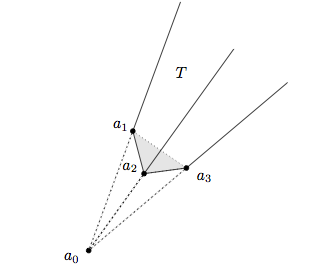
Let us go back now to the decomposition (27). We should also note that $M$, the number of infinite tetrahedra, is not intended to be large. This is just a domain decomposition of a $\Omega_{\infty}$ in which the subdomains are infinite tetrahedra and are fixed once for all. In practice, $M$ is often small ($M=3,4,...$). An example is illustrated in Figure 3 where $\Omega_{0}$ is a big tetrahedron centered at the origin and $\Omega_{\infty}$ is the union of $4$ infinite tetrahedra (see also section 4 hereafter). Another possibility consists to choose $\Omega_{0}$ as the octahedron $\{{\boldsymbol{x}}=(x_{1},x_{2},x_{3})\in{\mathbb{R}}^{3}\;|\;|x_{1}|+|x_{2}|+|x_{3}|<R\}$ and $\Omega_{\infty}={\mathbb{R}}^{3}\backslash\overline{\Omega_{0}}$ as the union of $8$ infinite tetrahedra (see Figure 2).

Subsequently, we denote by $S_{i}$, $1\leqslant i\leqslant M$, the tetrahedron associated to $T_{i}$ and by ${\boldsymbol{h}}_{i}$ the altitude vector corresponding of $T_{i}$. We have

Set

Since ${\boldsymbol{0}}$ is the fictitious vertex of each $T_{i}$ and in view of (28) it can easily be proved that

In terms of the local barycentric coordinates in $S_{i}$, $(\lambda^{(i)}_{0},\lambda^{(i)}_{1},\lambda^{(i)}_{2},\lambda^{(i)}_{3})$, we can write

The following continuity property holds true: if $T_{i}$ and $T_{j}$ are neighbors, then

The local polygonal inversion associated to $T$ is defined as

Obviously $\phi_{i}$ is a bijection between $S_{i}$ and $T_{i}$. It is also an involution which preserves $T_{i}\cap S_{i}$, that is $\phi_{i}({\boldsymbol{x}})={\boldsymbol{x}}$ for ${\boldsymbol{x}}\in T_{i}\cap S_{i}$.
Define now the global polygonal inversion $\phi$ from ${\mathbb{R}}^{3}\setminus\{0\}$ into itself and the global polygonal radius $r(.)$ as follows

In virtue of property (30), $r$ and $\phi$ are well defined and continuous on ${\mathbb{R}}^{3}$. Moreover, $\phi$ maps $\Omega_{\infty}$ into $\Omega_{0}$ and conversely. We have

Moreover, the exists two constants $c_{1}>0$ and $c_{2}>0$ such that

In other words, $r({\boldsymbol{x}})\sim|{\boldsymbol{x}}|$ and $|\phi({\boldsymbol{x}})|\sim{|{\boldsymbol{x}}|^{-1}}\mbox{ for }{\boldsymbol{x}}\in{\mathbb{R}}^{3}$. In the sequel, $\Omega_{\star}$ stands for the image of $\Omega_{\infty}$ by the inversion $\phi$. From a strictly mathematical point of view $\Omega_{\star}=\Omega_{0}\backslash\{{\boldsymbol{0}}\}$. However, since $\Omega_{0}$ and $\Omega_{\star}$ will be meshed differently. We will therefore deal with them separately.
We now consider a family of pairs of triangulations $({{\mathcal{T}}_{h}},{\mathcal{T}}_{h}^{\star})_{h}$ where

• •

  $({{\mathcal{T}}_{h}})_{h}$ are regular triangulations of $\Omega_{0}$ satisfying the usual conformity assumptions (see [5] or [7]). In particular, elements of ${{\mathcal{T}}_{h}}$ are supposed shape regular in the usual sense: there exists a constant $c_{0}>0$ not depending on $h$ such that

  (33)

  $$\max_{K\in{{\mathcal{T}}_{h}}\cup{\mathcal{T}}_{h}^{\star}}\frac{h_{K}}{\rho_{K}}\leqslant c_{0}.$$

  Here $h_{K}$ and $\rho_{K}$ are respectively the diameter of $K$ and the diameter of the sphere inscribed inside of the tetrahedron $K$.

• •

  $({\mathcal{T}}_{h}^{\star})_{h}$ are regular triangulations of $\Omega_{\star}$ which satisfies, besides (33), the following additional requirement:

  • –

    for each $K_{\star}\in{\mathcal{T}}_{h}^{\star}$, there exists $i\leqslant M$ such that $K_{\star}\subset S_{i}$ (in other words, ${\mathcal{T}}_{h}^{\star}$ is a conforming union of triangulations of the subdomains $S_{1}$,..,$S_{M}$).

  • –

    the triangulations $({\mathcal{T}}_{h}^{\star})_{h}$ are $\mu$-graded, where $\mu\in(0,1]$ is a fixed parameter. That means that there exists three constants $c^{\star}_{1}>0$, $c^{\star}_{2}>0$ and $c^{\star}_{3}>0$, not depending on $h$, such that

    (34)

    $$\max_{K\in{\mathcal{T}}_{h}^{\star\star}}\frac{h_{K}}{d^{1-\mu}_{K}}\leqslant c^{\star}_{1}h,\;$$

    (35)

    $$\max_{K\in{\mathcal{T}}_{h}^{\star}\backslash{\mathcal{T}}_{h}^{\star\star}}h_{K}\leqslant c^{\star}_{2}h^{1/\mu},\;$$

    (36)

    $$\min_{K_{\star}\in{\mathcal{T}}_{h}^{\star\star}}d_{K_{\star}}\geqslant c^{\star}_{3}h^{1/\mu},$$

    where ${\mathcal{T}}_{h}^{\star\star}=\{K\in{\mathcal{T}}_{h}^{\star}\;|\;{\boldsymbol{0}}\not\in K\}$ (elements not touching the origin), $d_{K}=\inf_{{\boldsymbol{x}}\in K}|{{\boldsymbol{x}}}|$ for all $K\in{\mathcal{T}}_{h}^{\star}$, and

    $$h=h({{\mathcal{T}}_{h}},{\mathcal{T}}_{h}^{\star})=\max_{K\in{{\mathcal{T}}_{h}}\cup{\mathcal{T}}_{h}^{\star}}h_{K},$$

  Conditions (34), (35) and (36) mean that tetrahedra of ${\mathcal{T}}_{h}^{\star}$ which are adjacent to $\partial\Omega_{\star}\cap\partial\Omega_{\infty}$ have a size of order $h$, while those touching the fictitious vertex ${\boldsymbol{0}}$ have a size of order $h^{1/\mu}$. Construction of graded meshes is detailed in [5].

• •

  ${{\mathcal{T}}_{h}}$ and ${\mathcal{T}}_{h}^{\star}$ have the same vertices, edges and faces on the common boundary $\Omega_{0}\cap\Omega_{\infty}=\partial\Omega_{0}=\partial\Omega_{\star}\backslash\{0\}$.

In the sequel, given a function ${\boldsymbol{v}}$ defined over $\Omega_{\infty}$, ${\hat{v}}$ stands for the function defined on $\Omega_{\star}$ as follows

with $\gamma>0$ a parameter. Conversely, we have

Now, let $k\geqslant 1$ be a fixed integer and consider the finite dimensional space

We may observe that functions of $W_{h}$ are piecewise polynomial in the FEM region $\Omega_{0}$, but not in the IFEM region $\Omega_{\infty}$. The last observation is due to distorsion resulting from the composition with the inversion and the multiplicative factor involved in formula (37).
Another observation concerns the behavior at large distances of functions belonging to $W_{h}$. Let ${v}\in W_{h}$. Then, $v\in H^{1}_{loc}({\mathbb{R}}^{3})^{3}$. Moreover, since ${\hat{v}}({\boldsymbol{0}})=0$, we have

for some constant $C_{0}$, not depending on ${\boldsymbol{x}}_{\star}$. It follows that for all ${\boldsymbol{x}}\in\Omega_{\infty}$, we have

In similar way, we prove that

We deduce this

This justifies the following assumption on $\gamma$:

The discrete problem writes: find $u_{h}\in W_{h}$ such that

The corresponding stray-field energy is given by

We have

Proposition 3.1 states in particular that if $u\in W^{k+1}_{k+\gamma}({\mathbb{R}}^{3})$ and if the mesh of $\Omega_{\star}$ is graded enough ($\mu\leqslant\frac{\eta}{k}$), then the error is similar to that held in the finite element method in bounded domains, that is

We also have

When smoothness of $u$ is only local, we have this

References

- [1] F. Alliot. Etude des équations stationnaires de Stokes et Navier-Stokes dans des domaines extérieurs. PhD Thesis, ENPC, Paris, 1998.
- [2] C. Amrouche, V. Girault, and J. Giroire. Weighted Sobolev spaces for Laplace’s equation in . J. Math. Pures Appl. (9), 73(6):579–606, 1994.
- [3] D. V. Berkov, K. Ramstöck, and A. Hubert. Solving micromagnetic problems: toward and optimal numerical method. Phys. Stat. Sol (a), 137:207–225, 1993.
- [4] J. L. Blue and M. R. Scheinfein. Using multipoles decreases computation time for magnetic self-energy. IEEE Trans. Magn., 27:4778–4780, 1991.
- [5] T. Z. Boulmezaoud. Inverted finite elements: a new method for solving elliptic problems in unbounded domains. M2AN Math. Model. Numer. Anal., 39(1):109–145, 2005.
- [6] C. Carstensen and A. Prohl. Numerical analysis of relaxed micromagnetics by penalised finite elements. Numer. Math., 90(1):65–99, 2001.
- [7] Ph.-G. Ciarlet. The finite element method for elliptic problems. North-Holland Publishing Co., Amsterdam, 1978.
- [8] A. Class, L. Exl, G. Selke, A. Drews, and Th. Schrefl. Fast stray field computation on tensor grids. Journal of magnetism and magnetic materials, 176(326), 2013.
- [9] L. Exl, W. Auzinger, S. Bance, M. Gusenbauer, F. Reichel, and T. Schrefl. Fast stray field computation on tensor grids. J. Comput. Phys., 231(7):2840–2850, 2012.
- [10] D. R. Fredkin and T. R. Koehler. Hybrid method for computing demagnetizing fields. IEEE Trans. Magn., 26:415–417, 1990.
- [11] J. Giroire. Etude de quelques problèmes aux limites extérieurs et résolution par équations intégrales. Thèse de Doctorat d’Etat. Université Pierre et Marie Curie, Paris, 1987.
- [12] H. Han and W. Bao. The discrete artificial boundary condition on a polygonal artificial boundary for the exterior problem of Poisson equation by using the direct method of lines. Comput. Methods Appl. Mech. Engrg., 179(3-4):345–360, 1999.
- [13] H. Han and W. Bao. Error estimates for the finite element approximation of problems in unbounded domains. SIAM J. Numer. Anal., 37(4):1101–1119, 2000.
- [14] B. Hanouzet. Espaces de Sobolev avec poids application au problème de Dirichlet dans un demi espace. Rend. Sem. Mat. Univ. Padova, 46:227–272, 1971.
- [15] T. R. Koehler and D. R. Fredkin. Finite element methods for micromagnetism. IEEE Trans. Magn., 28:1239–1244, 1992.
- [16] S. Labbé. Fast computation for large magnetostatic systems adapted for micromagnetism. SIAM J. Sci. Comput., 26(6):2160–2175, 2005.
- [17] H. Long, E. Ong, Z. Liu, and E. Li. Fast fourier transform on multipoles for rapid calculation of magnetostatic fields. IEEE Trans. Magn., 42:295–300, 2006.
- [18] M. Luskin and L. Ma. Analysis of the finite element approximation of microstructure in micromagnetics. SIAM J. Numer. Anal., 29(2):320–331, 1992.
- [19] J.-C. Nédélec. Acoustic and electromagnetic equations, volume 144 of Applied Mathematical Sciences. Springer-Verlag, New York, 2001. Integral representations for harmonic problems.
- [20] N. Popović and D. Praetorius. Applications of -matrix techniques in micromagnetics. Computing, 74(3):177–204, 2005.
- [21] A. Prohl. Computational micromagnetism. Advances in Numerical Mathematics. B. G. Teubner, Stuttgart, 2001.