Construction of Uniform Designs over Continuous Domain in Computer Experiments
Abstract
Construction of uniform designs (UDs) has received much attention in computer experiments over the past decades, but most of previous works obtain uniform designs over a U-type by lattice domain. Due to increasing demands for continuous factors, UDs over continuous domain is in lack. Moreover, the uniformity can be further improved over a continuous domain. In this paper, we use coordinate descent methods with an initialization derived by threshold accepting (TA) algorithm to construct UDs over continuous domain with Centered -discrepancy. The new UDs perform better than the recorded ones in several computer experiments by the Kriging modeling.
Keywords: Centered -discrepancy, Computer experiment, Coordinate descent, Kriging modeling, Lattice point, Threshold accepting, Uniform designs
MSC: 62K05; 62K15
1 Introduction
With the development of science and technology, computer experiments have gained more and more attention in recent years. Engineers and scientists implement computer simulations on physical systems due to the complex relationships between the inputs and outputs. Fang et al., 2005 gave a comprehensive introduction to the design and modeling of computer experiments. In computer experiments, the true underlying model
| (1) |
is known and usually too complicated to conduct some computation demanding works such as sensitivity analysis and optimization, where the response depends on the factors in the experimental domain . For a given input representing experimental runs, one can obtain their output from the true model (1). Based on the observations of the data set , an approximate model
| (2) |
called metamodel is built and used for some applications such as optimization and sensitivity analysis. There are various modeling techniques such as Kriging models, (orthogonal) polynomial regress models, Bayesian methods and neural networks. More details can be found in Fang et al., 2005.
There are two key issues in computer experiments: design and modeling. The so-called space filling design has been recommended for computer experiments. The Latin hypercube sampling (LHS) proposed by McKay et al., 1979 is one of the most popular space filling design. With design points uniformly scattered on the experimental domain, the uniform design proposed by Fang, 1980, Wang and Fang, 1981 is another widely used space-filling design.
The Latin hypercube sampling and uniform design are based on the estimation of overall mean of :
where follows the uniform distribution on . Then can be estimated by the mean . LHS provides a more efficient estimate of than the estimate by the simple random sampling. The Koksma-Hlawka inequality (see Hua and Wang, 1981) gives the upper error bounds of the estimate as
| (3) |
where is a measure of the variation of , and is the star-discrepancy of , a measure of the uniformity of . The definition of is in the sense of Hardy and Krause (Hua and Wang, 1981). Note that is independent of the design points. Thus, given a bounded , inequality (3) indicates that the more uniform a set of points is over the experimental region , the more accurate is as an estimator of . The uniform design is based on this overall mean model.
When the factors are quantitative and their domain is a rectangle , without loss of generality, we can assume the experimental domain is a unit cube . To measure the uniformity, Hickernell, 1998 proposed some new discrepancies such as Centered -discrepancy (CD) and wrap-around -discrepancy (WD) to replace the star-discrepancy. Zhou et al., 2013 also suggested mixture discrepancy (MD). In this paper, we adopt CD. The squared CD has a computational formula
| (4) |
where is from a unit hypercube . The uniform design is defined as follows.
Definition 1.
For an experiment consists of runs relating to factors on an experimental region , denote the experimental domain by that is collection of sets . Then a design, , is called a uniform design under a given measure discrepancy if
| (5) |
Constructing a uniform design is an NP hard problem that there is no exact algorithm for global optima within polynomial time. Besides, in practical experiments, the feasible values of factors are limited so that the corresponding levels in designs are required to be discrete. Therefore, for construction of uniform designs, traditional methods often focused on a lattice domain instead of the full set . The U-type domain is prevalently accepted in existing literatures.
Definition 2.
Suppose a design is an matrix. Then it is said to be a q-level U-type design denoted as if in each column of , the entries, for , appear equally often.
Most of authors restrict a U-type design in an experimental region, , defined in Definition 2. The uniform design obtained from a U-type domain is called U-type uniform design, denoted as . There are many construction approaches to , such as the good lattice point method, the combinatorial construction method, cutting method, and the foldover technique. Stochastic optimization algorithm is also feasible for this problem. More details can refer to Fang et al., 2018.
The threshold accepting (TA) algorithm proposed by Dueck and Scheuer, 1990, is a variation of the more widely used simulated annealing (SA) algorithm, that proposed by Kirkpatrick, 1984 through the emulation of the physical annealing process in solids. However, since SA algorithm involves too many parameters for the user choosing, its process convergence is slow. Hence in many cases, TA as a descendent has better performance than SA since it provides quicker convergence and better results during the same computational time. Multivariate or combinatorial optimization problems, including some NP-complete or NP-hard problems, have been tackled through TA, such as portfolio optimization problem (Dueck and Winker, 1992), NP-complete problem of optimal aggregation (Chipman and Winker, 1995) and NP-hard traveling salesman problem (Winker, 1994).
Referred to the definition of a uniform design in (5), generating a UD is a large scale integer programming problem with multimodal objective function ( discrepancies) over a discrete, large and complicated domain ( experimental region). Winker and Fang, 1997 and Winker and Fang, 1998 firstly applied the TA to the calculation of the star discrepancy and construction of uniform designs on the lattice domain. Fang et al., 2017 discussed how to apply TA to construction of orthogonal designs. Most uniform designs recorded on the website https://dst.uic.edu.cn/en/isci/uniform-design/uniform-design-tables have been obtained by TA algorithm.
Computer simulations play a dominant role in modern applications. Traditional computer experimental designs are in a lattice domain, in which the factors of interest are limited with discrete levels in experiments. However, with the improvement of computational ability, factors in practical may refer to a continuous domain, that leads to a great loss of information if the experimenter still choose a design from a lattice domain. The uniform designs over continuous domain are suitable for this case, and easily to be carried out. They should have better uniformity than U-type UDs as well, and as consequence, perform better in modeling. Hence, construction of uniform designs over continuous domain is in badly need. Our paper is to propose an approach to obtaining the UDs over continuous domain, especially in a rectangle. Finding a uniform design in a continuous is a high dimensional non-convex optimization problems. Here we only consider the case in which in Definition 2. For a point set from , the objective is to minimize the square of CD (1):
| (6) |
Gradient descent (Ruder, 2016) is a good way to solve such problems with a suitable initialization. However, it costs too much for large sized designs (i.e. and are large), which are prevalent in computer experiments. Coordinate descent (Wright, 2015) is also feasible for this problem. Compared with gradient descent, the coordinate update is simpler and cheaper, especially for the high dimensional optimization problems. Choosing a suitable initial design is very important, in this paper we adopt initial designs obtained from TA. An introduction of TA algorithm is given in Section 2. In Section 3, the implementation on constructing uniform designs through coordinate descent methods are conducted, in which iteration formula of CD is feasible to facilitate the efficiency of algorithm. To evaluate the modeling performance of new uniform designs over continuous domain, we adopt several case studies of computer experiments in Section 4.
2 Constructing Uniform Designs through TA Algorithm
The TA algorithm starts with an arbitrarily generated U-type design, say , and then it performs a large number of iterations. During each iteration, a new solution is generated and used for substituting the current solution, say , while in the first iteration . The new solution is derived from a so-called neighborhood of the current solution , which is often defined as a small permutation of the current solution. A decision rule in each iteration is to determine whether to accept the new solution and update the current objective function value or not. We present the flow chart of TA algorithm for generating uniform designs in Figure 1.

hreshold Accepting Algorithm for Generating Uniform Designs
In uniform design construction, the purpose is to minimize the discrepancy. Hence, in each iteration, the results of the new candidate and the current solution are compared through . A trivial local search algorithm accepts if and only if . In this algorithm, the resulting solution has a large probability that gets stuck in a bad local optimum especially as the objective function is multimodal. Winker and Fang, 1998 indicated that in the application to the traveling salesman problem, the result quality of the trivial local search algorithm got stuck in a bad level and could not be improved by further increasing the number of iterations. Therefore, TA adopts another acceptance criterion that allows certain temporary worsening with respect to a predetermined threshold value, say . That implies in each iteration, a new candidate is accepted if and only if . Thus TA is also regarded as the refined local search algorithm.
The threshold value is not a constant but a finite sequence that is positive and decreasing to zero. As the threshold value is nonzero in most of the iterations, even if the current solution is stuck in a bad local optimum, it has chance to leave. At the very end, the threshold value ends up at zero, that ensures the solution of TA algorithm is still a local optimum. But the local optimum of TA has high quality and at least is approaching to the global optimum.
The key of TA algorithm is to define the neighborhood and threshold sequence. A U-type design is regarded as a neighborhood of the current design if they differ by elements in at most columns. Many authors set , and define each neighborhood by randomly exchanging two elements in a randomly chosen column of the current design (so-called TA neighborhood). The definition of the neighborhoods provides an endogenous data-driven approach to generating a threshold sequence. In this paper, we adopt a recursive formula
to derive the threshold sequence in an exponentially decreasing manner, refer to Fang et al., 2017. With the given parameters , and , the procedure of generating a threshold sequence is as follows:
- (1)
generate the initial design of the TA algorithm, ;
- (2)
find neighborhoods of the initial design, , ;
- (3)
calculate the squared CD values for each neighborhood, ;
- (4)
compute the range of the squared CD values of the neighborhoods,
; - (5)
set threshold basis and ;
- (6)
generate the rest threshold sequence through , .
However, the definition of TA neighborhood is for the convenience of computation. It is different from the mathematical neighborhood with respect to CD function. For instance, considering the uniform design recorded on the website mentioned before, Figure 2 gives the distributions of CD values of designs in different neighborhoods. The right box-plot in Figure 2 plots the CD values of TA neighborhoods of . The left box-plot is for the designs derived by level permutation on randomly chosen one column of . The CD value of TA neighborhoods may vary from each other in a great amount, compared to level permuted designs. Hence, this definition of neighborhood is not feasible for continuous uniform designs.

A: The box-plot of in level permutation of one randomly chosen column of .
B: The box-plot of in level-permutation neighborhood
3 Coordinate Descent Algorithms with TA Initialization
Coordinate descent algorithms are a class of large-scale optimization algorithms that are feasible for various objective functions including non-smooth and non-convex ones. They have been successfully implemented on the problems in various modern applications such as machine learning and large-scale computational statistics. For some structured problems, coordinate descent algorithms have shown advantage on computation speed and convergence proof over traditional algorithms, such as gradient descent (GD), refer to Shi et al., 2016. A comprehensive introduction with applications to coordinate descent variants has been elaborated by Wright, 2015 and Shi et al., 2016. In this paper, three coordinate descent algorithms are introduced and discussed on their performance in constructing UDs.
Recall in (6) that constructing a uniform design under CD is an optimization problem with non-convex objective function,
where the objective function indicating CD in (1) has the second derivative, and . In traditional gradient optimization algorithm, there are two possible actions in each iteration. Coordinate descent is a simple but efficient non-gradient optimization algorithm. The gradient optimization algorithm seeks for the minimum value of the function along the direction of the most rapid descent. However, coordinate descent minimizes the value of the objective function along the coordinate gradient in each step.
3.1 Coordinate Gradient Descent (CGD)
To construct a UD, , the optimization problem can be regarded as an -dimensional problem with points on . An uniform design matrix can be viewed as design points each having dimension. Coordinate gradient descent is to adjust the position of each design point in each dimension so that the whole design point set can be more uniformly distributed in the domain. Figure 3 visualizes the design points during the optimization process. Figure 4 presents the design points of from any two-dimensional projection points. The visualization figures may help us comprehend the objective uniformity measure CD adopted in this paper. The figures indicate that the whole design points become centrally aggregated after coordinate descent. The following algorithm is the basic coordinate gradient descent method.


3.2 Coordinate Zero-gradient (CZG)
Since the coordinate gradient in Algorithm 1, , is known, we can set to find the coordinate value while fixing other coordinate values.
| (7) |
where the sgn function is:
| (8) |
The coordinate value, , can be derived through taking . However, some of in sgn function can not be solved through explicit expression. Here we adopt recursion with an initialization, denoted as , and a maximum number of iterations, , while other coordinate values , are fixed. The recursive formula is given as
| (9) |
where
| (10) |
and
| (11) |
for . Through plenty of experiments, is enough for getting good results.
In our experiments, the coordinate zero-gradient method is advantaged in computation speed. For the same optimization task, it takes several minutes through coordinate gradient descent method but several seconds through coordinate zero-gradient method. However, even though the final optimization result is good enough, the CD values during the optimization process is unstable. For instance, sometimes there may be violent fluctuations of the CD values.
3.3 Coordinate Descent with Fixed Step Size (CDFSS)
Considering the limit of minimum unit of variables in practical experiments, coordinate descent with fixed step size are suitable under such circumstances. The idea of this method is to replace the coordinate gradient with and the step size can be set as the minimum unit of variables. In each step, the coordinate with the rapidest descent will be chosen. The algorithm will be stopped until there is no further descent in any coordinate.
This method can be easily applied in the experiments with minimum unit due to the equipment or technology limitations. For example, one of the variable, temperature, in the industry experiment is from 0 to T. Due to the limitations of temperature detection and control technology, the minimum unit is 0.1 degree. With CDFSS, the step size of the variable can be set as . Similarly for other variables, the step size can be set different values according to the corresponding limitations. Thus, the resulted uniform design is feasible under practical experimental requirements.
Actually, in the experiments, these three algorithms may get different results with the same initialization. With the same initialization, the aforementioned three algorithms are conducted respectively. We present the CD values in Table 1. Table 1 shows that the final uniform designs of these algorithms may be different due to the complexity of non-convex high dimensional optimization. But using better initialization ( on the website) facilitates the optimization process.
| Website | ||
|---|---|---|
| GD | 0.033972 | 0.052300 |
| CGD | 0.033972 | 0.041678 |
| CZG | 0.033972 | 0.052690 |
| CDFSS | 0.033972 | 0.042079 |
3.4 TA Initialization
Due to the non-convexity of in (1), the initialization is significant in the gradient-based methods. With different initialization, various local minimum will be achieved by using the same coordinate descent algorithm. For example, when constructing through different initial designs, coordinate gradient descent obtains different results shown in Table 2.
| Initialization type | |
|---|---|
| 0.041678 | |
| 0.061949 | |
| 0.041114 | |
| 0.041227 | |
| on website | 0.033972 |
TA algorithm has successfully obtained many uniform designs over the U-type lattice point domain on the website mentioned above. Hence, intuitively we adopt the uniform design derived by TA algorithm as the initialization. Then subsequently, we conduct the coordinate descent methods to optimize the uniform designs over a continuous domain, . Table 3 presents the CD values of uniform designs derived by TA over a U-type domain and by TA+CGD over a continuous domain. The CD values can be further improved over a continuous domain through coordinate descent methods, compared to the existing UDs on the website.
| Algorithms | ||
|---|---|---|
| TA | 0.035403 | 0.228455 |
| TA + CGD | 0.033972 | 0.198073 |
| 0.9080 | 0.5238 | 0.6906 | 0.8001 | 0.7509 | 0.3578 | 0.9071 |
| 0.3050 | 0.5838 | 0.6351 | 0.0531 | 0.6986 | 0.7447 | 0.1393 |
| 0.7475 | 0.2567 | 0.4738 | 0.2078 | 0.9052 | 0.8544 | 0.6415 |
| 0.9457 | 0.1462 | 0.3609 | 0.4796 | 0.3579 | 0.6288 | 0.0542 |
| 0.4704 | 0.6925 | 0.5757 | 0.9079 | 0.1977 | 0.2049 | 0.0972 |
| 0.1438 | 0.4809 | 0.0946 | 0.2525 | 0.0549 | 0.5210 | 0.2979 |
| 0.5264 | 0.0986 | 0.8501 | 0.1441 | 0.1533 | 0.4260 | 0.7990 |
| 0.3570 | 0.0529 | 0.1464 | 0.5804 | 0.8045 | 0.2527 | 0.4264 |
| 0.0957 | 0.7482 | 0.9468 | 0.5135 | 0.8528 | 0.5862 | 0.5889 |
| 0.6366 | 0.4197 | 0.0528 | 0.9471 | 0.5825 | 0.6931 | 0.7531 |
| 0.0546 | 0.3076 | 0.4149 | 0.6973 | 0.3062 | 0.0959 | 0.6922 |
| 0.2009 | 0.1964 | 0.7458 | 0.8505 | 0.4748 | 0.9032 | 0.3564 |
| 0.7971 | 0.8605 | 0.8011 | 0.6355 | 0.0960 | 0.7947 | 0.4694 |
| 0.4159 | 0.6462 | 0.2524 | 0.4225 | 0.2570 | 0.9456 | 0.9456 |
| 0.5711 | 0.9058 | 0.2994 | 0.7430 | 0.9456 | 0.4756 | 0.2040 |
| 0.2435 | 0.9512 | 0.5211 | 0.3061 | 0.5330 | 0.3026 | 0.8508 |
| 0.6876 | 0.3689 | 0.9043 | 0.3633 | 0.6321 | 0.0539 | 0.2502 |
| 0.8534 | 0.7923 | 0.1928 | 0.0974 | 0.4286 | 0.1500 | 0.5260 |
| 0.0971 | 0.8438 | 0.2913 | 0.5290 | 0.7735 | 0.4409 | 0.8424 | 0.6708 | 0.4005 | 0.1238 | 0.3293 | 0.6793 | 0.8683 |
| 0.5663 | 0.8711 | 0.7423 | 0.3992 | 0.1332 | 0.1908 | 0.1838 | 0.3580 | 0.5025 | 0.8424 | 0.5971 | 0.7083 | 0.0939 |
| 0.7020 | 0.0962 | 0.2268 | 0.1853 | 0.5957 | 0.3299 | 0.5591 | 0.0915 | 0.1942 | 0.4693 | 0.6391 | 0.7802 | 0.7763 |
| 0.1914 | 0.5124 | 0.6684 | 0.7741 | 0.5287 | 0.1272 | 0.2272 | 0.2965 | 0.3338 | 0.2203 | 0.8354 | 0.2634 | 0.8097 |
| 0.2906 | 0.2188 | 0.4044 | 0.3498 | 0.6775 | 0.1570 | 0.9011 | 0.1962 | 0.8988 | 0.5647 | 0.4023 | 0.3885 | 0.1243 |
| 0.4771 | 0.1907 | 0.8427 | 0.9289 | 0.7377 | 0.9084 | 0.0971 | 0.5278 | 0.2559 | 0.4013 | 0.4324 | 0.7423 | 0.5594 |
| 0.3673 | 0.1224 | 0.8728 | 0.6715 | 0.3999 | 0.2237 | 0.6704 | 0.8715 | 0.6986 | 0.8150 | 0.2553 | 0.5226 | 0.7389 |
| 0.8424 | 0.4354 | 0.9068 | 0.8085 | 0.9281 | 0.4679 | 0.7395 | 0.1242 | 0.4656 | 0.7069 | 0.5278 | 0.1253 | 0.4302 |
| 0.0717 | 0.1596 | 0.2587 | 0.2915 | 0.2922 | 0.5324 | 0.3007 | 0.5610 | 0.5250 | 0.9289 | 0.8047 | 0.0925 | 0.5224 |
| 0.2272 | 0.6788 | 0.5259 | 0.7056 | 0.0705 | 0.8810 | 0.6402 | 0.1554 | 0.6313 | 0.6011 | 0.9295 | 0.6398 | 0.6283 |
| 0.9267 | 0.7367 | 0.8156 | 0.3238 | 0.2645 | 0.5657 | 0.3593 | 0.2191 | 0.1246 | 0.0966 | 0.3680 | 0.5100 | 0.6731 |
| 0.9006 | 0.3594 | 0.1018 | 0.4724 | 0.8127 | 0.2550 | 0.1526 | 0.7021 | 0.6665 | 0.2897 | 0.9045 | 0.5622 | 0.3623 |
| 0.6695 | 0.0708 | 0.4881 | 0.6381 | 0.5080 | 0.8414 | 0.4007 | 0.9288 | 0.4352 | 0.0711 | 0.6766 | 0.3326 | 0.0710 |
| 0.5170 | 0.4010 | 0.4748 | 0.1214 | 0.0934 | 0.4096 | 0.0724 | 0.7373 | 0.2922 | 0.6378 | 0.1547 | 0.3624 | 0.9275 |
| 0.1574 | 0.3288 | 0.6032 | 0.4884 | 0.8388 | 0.7119 | 0.4358 | 0.2642 | 0.0962 | 0.8977 | 0.0973 | 0.5941 | 0.2872 |
| 0.6397 | 0.8051 | 0.1902 | 0.9022 | 0.7080 | 0.5996 | 0.4721 | 0.4047 | 0.8367 | 0.8721 | 0.7358 | 0.4241 | 0.9042 |
| 0.8098 | 0.7682 | 0.6383 | 0.7497 | 0.5623 | 0.3728 | 0.3233 | 0.7705 | 0.9292 | 0.5323 | 0.1828 | 0.8078 | 0.2576 |
| 0.4356 | 0.9014 | 0.7820 | 0.2190 | 0.6455 | 0.6712 | 0.8026 | 0.8402 | 0.2229 | 0.5137 | 0.8732 | 0.2930 | 0.3339 |
| 0.5292 | 0.2573 | 0.1643 | 0.8350 | 0.2219 | 0.6356 | 0.7776 | 0.3306 | 0.5549 | 0.1957 | 0.1271 | 0.8760 | 0.3938 |
| 0.3232 | 0.5606 | 0.3683 | 0.2547 | 0.9073 | 0.8088 | 0.2573 | 0.9027 | 0.7356 | 0.6824 | 0.5189 | 0.9025 | 0.6990 |
| 0.1306 | 0.4634 | 0.9265 | 0.0734 | 0.3654 | 0.4859 | 0.5235 | 0.4446 | 0.8092 | 0.1592 | 0.7133 | 0.8388 | 0.2217 |
| 0.4013 | 0.9279 | 0.3244 | 0.5670 | 0.4259 | 0.7460 | 0.1239 | 0.0721 | 0.7729 | 0.3316 | 0.2306 | 0.1871 | 0.4684 |
| 0.8678 | 0.5964 | 0.0736 | 0.0967 | 0.4722 | 0.9262 | 0.7000 | 0.4762 | 0.3608 | 0.7794 | 0.2910 | 0.4719 | 0.1625 |
| 0.7417 | 0.5304 | 0.4385 | 0.6016 | 0.3333 | 0.0932 | 0.9281 | 0.5975 | 0.0718 | 0.7427 | 0.7742 | 0.9281 | 0.5089 |
| 0.7788 | 0.3003 | 0.7021 | 0.4343 | 0.1600 | 0.7792 | 0.8683 | 0.6321 | 0.8693 | 0.3659 | 0.5660 | 0.2166 | 0.8376 |
| 0.2576 | 0.6397 | 0.1321 | 0.8754 | 0.1864 | 0.2929 | 0.5135 | 0.8070 | 0.1546 | 0.4325 | 0.4745 | 0.1554 | 0.1941 |
| 0.6064 | 0.6963 | 0.5617 | 0.1565 | 0.8705 | 0.0711 | 0.5982 | 0.5135 | 0.5994 | 0.2536 | 0.0715 | 0.0715 | 0.5914 |
To further explore the performance of new uniform designs, we implement them on several computer experiments in the next section. In these case studies, we use Kriging modeling technique to obtain an approximate model for responses and factors. We evaluate the mean squared errors (MSE) when predicting untried points through the approximate models trained by the new uniform designs, compared with the ones recorded on the website, and the Latin hypercube sampling.
4 Modeling Performance of Uniform designs over Continuous Domain
The question is requested whether the new uniform designs with smaller CD on the continuous domain has better performance in modeling. We apply the new uniform designs in several computer experiments as case studies. There are many modeling techniques among which we adopt Kriging modeling technique in this study. Fang et al., 2005 gave an elaborate introduction to Kriging models.
Definition 3.
Suppose that are design points over an -dimensional experimental domain, and is the corresponding output. The universal Gaussian Kriging model is defined as
where the set of is a chosen polynomial basis over the design region and is a Gaussian process. The ordinary Kriging model is the most commonly used in practice, defined as
where is the overall mean of .
DACE packakge in MATLAB is employed for Kriging modeling. There are several candidate basis in this package, such as Poly0 representing ordinary Kriging models, Poly1 representing first-order polynomial function as basis, and Poly2 representing second-order polynomial function as basis. We evaluate the modeling performance through comparing the prediction MSE on untried points of Kriging models trained by the new uniform designs and the recorded ones in the website. The MSE is defined as follows.
Since Latin hypercube sampling (LHS) has been popular in computer experiments, we also provide the prediction MSE of the Kriging models trained by LHS and mid-point LHS (MLHS), defined in Definition 5. Since each LHS or MLHS is a random sample, we generate ten LHS or MLHS each time and conduct Kriging modeling respectively. Subsequently, we present the average prediction MSE of each Kriging model trained by these ten LHS or MLHS, denoted as Avg. LHS or Avg. MLHS in Table 7 and 8.
Definition 4.
A Latin hypercube design (LHD) with runs and factors, denoted by , is an matrix, in which each column is a random permutation of 1,2,…,n.
Definition 5.
Let , , denote the permutations of . Take mutually independent uniform random variables , , . Let , where , . Then is a LHS and denoted by . If for each , we fix at a mid-point instead of a random number, that is , is a mid-point LHS, denoted as MLHS.
4.1 Wood Model
A wood function is notorious due to its difficulty on optimization, defined by
for . The global minimum is at with . We apply several new uniform designs over continuous domain, denoted as , and the corresponding recorded ones, on the website respectively into wood model, in which 9-run and 16-run designs shown in Table 6.
| 4 | 1 | 7 | 5 | -0.5 | -2 | 1 | 0 | 0.3942 | 0.0690 | 0.7114 | 0.5978 | -0.4232 | -1.7242 | 0.8457 | 0.3912 |
|---|---|---|---|---|---|---|---|---|---|---|---|---|---|---|---|
| 1 | 3 | 4 | 3 | -2 | -1 | -0.5 | -1 | 0.0743 | 0.2762 | 0.3966 | 0.2761 | -1.7030 | -0.8953 | -0.4136 | -0.8957 |
| 9 | 9 | 5 | 4 | 2 | 2 | 0 | -0.5 | 0.9303 | 0.7215 | 0.6060 | 0.3940 | 1.7214 | 0.8861 | 0.4240 | -0.4240 |
| 6 | 6 | 6 | 9 | 0.5 | 0.5 | 0.5 | 2 | 0.6086 | 0.5114 | 0.4910 | 0.7172 | 0.4344 | 0.0456 | -0.0360 | 0.8689 |
| 5 | 7 | 2 | 1 | 0 | 1 | -1.5 | -2 | 0.5000 | 0.9207 | 0.2751 | 0.0793 | 0.0000 | 1.6830 | -0.8997 | -1.6830 |
| 2 | 8 | 8 | 7 | -1.5 | 1.5 | 1.5 | 1 | 0.1758 | 0.8242 | 0.8242 | 0.8242 | -1.2969 | 1.2969 | 1.2969 | 1.2969 |
| 3 | 5 | 1 | 6 | -1 | 0 | -2 | 0.5 | 0.2837 | 0.6065 | 0.0658 | 0.5000 | -0.8653 | 0.4260 | -1.7370 | 0.0000 |
| 8 | 2 | 3 | 8 | 1.5 | -1.5 | -1 | 1.5 | 0.8208 | 0.1875 | 0.1792 | 0.9065 | 1.2833 | -1.2501 | -1.2833 | 1.6262 |
| 7 | 4 | 9 | 2 | 1 | -0.5 | 2 | -1.5 | 0.7127 | 0.3945 | 0.9214 | 0.1705 | 0.8509 | -0.4220 | 1.6858 | -1.3181 |
| 1 | 10 | 4 | 6 | -2.00 | 0.40 | -1.20 | -0.67 | 0.4678 | 0.6593 | 0.4717 | 0.7195 | -0.1290 | 0.6370 | -0.1134 | 0.8778 |
| 2 | 4 | 13 | 15 | -1.73 | -1.20 | 1.20 | 1.73 | 0.2873 | 0.3469 | 0.0440 | 0.7769 | -0.8510 | -0.6126 | -1.8242 | 1.1074 |
| 3 | 13 | 10 | 10 | -1.47 | 1.20 | 0.40 | 0.40 | 0.1599 | 0.7847 | 0.5913 | 0.5975 | -1.3606 | 1.1386 | 0.3650 | 0.3898 |
| 4 | 8 | 7 | 1 | -1.20 | -0.13 | -0.40 | -2.00 | 0.0415 | 0.5965 | 0.2213 | 0.3425 | -1.8342 | 0.3858 | -1.1150 | -0.6302 |
| 5 | 6 | 1 | 2 | -0.93 | -0.67 | -2.00 | -1.73 | 0.7808 | 0.0927 | 0.3474 | 0.6514 | 1.1230 | -1.6294 | -0.6106 | 0.6054 |
| 6 | 15 | 15 | 4 | -0.67 | 1.73 | 1.73 | -1.20 | 0.2165 | 0.4656 | 0.4057 | 0.0389 | -1.1342 | -0.1378 | -0.3774 | -1.8446 |
| 7 | 1 | 11 | 7 | -0.40 | -2.00 | 0.67 | -0.40 | 0.7252 | 0.7091 | 0.9508 | 0.0981 | 0.9006 | 0.8362 | 1.8030 | -1.6078 |
| 8 | 16 | 8 | 14 | -0.13 | 2.00 | -0.13 | 1.47 | 0.3397 | 0.9060 | 0.7747 | 0.2254 | -0.6414 | 1.6238 | 1.0986 | -1.0986 |
| 9 | 3 | 3 | 3 | 0.13 | -1.47 | -1.47 | -1.47 | 0.8519 | 0.5300 | 0.7172 | 0.8348 | 1.4074 | 0.1198 | 0.8686 | 1.3390 |
| 10 | 7 | 16 | 9 | 0.40 | -0.40 | 2.00 | 0.13 | 0.6437 | 0.9514 | 0.2860 | 0.9514 | 0.5746 | 1.8054 | -0.8562 | 1.8054 |
| 11 | 11 | 5 | 16 | 0.67 | 0.67 | -0.93 | 2.00 | 0.4103 | 0.0373 | 0.6566 | 0.4060 | -0.3590 | -1.8510 | 0.6262 | -0.3762 |
| 12 | 12 | 12 | 2 | 0.93 | 0.93 | 0.93 | -1.73 | 0.5944 | 0.4045 | 0.8392 | 0.5308 | 0.3774 | -0.3822 | 1.3566 | 0.1230 |
| 13 | 2 | 6 | 11 | 1.20 | -1.73 | -0.67 | 0.67 | 0.9013 | 0.8316 | 0.0971 | 0.4668 | 1.6050 | 1.3262 | -1.6118 | -0.1330 |
| 14 | 14 | 2 | 8 | 1.47 | 1.47 | -1.73 | -0.13 | 0.9600 | 0.2836 | 0.5329 | 0.2779 | 1.8398 | -0.8658 | 0.1314 | -0.8886 |
| 15 | 9 | 14 | 13 | 1.73 | 0.13 | 1.47 | 1.20 | 0.5341 | 0.2096 | 0.1563 | 0.1535 | 0.1362 | -1.1618 | -1.3750 | -1.3862 |
| 16 | 5 | 9 | 5 | 2.00 | -0.93 | 0.13 | -0.93 | 0.1032 | 0.1681 | 0.8969 | 0.8969 | -1.5874 | -1.3278 | 1.5874 | 1.5874 |
| Avg. | Avg. | |||
|---|---|---|---|---|
| Poly0 | 957.9618 | 826.0637 | 816.8131 | 805.1325 |
| Poly1 | 878.1982 | 695.0498 | 877.2432 | 847.6947 |
| Avg. | Avg. | |||
| Poly0 | 829.4668 | 743.3496 | 672.0404 | 725.3436 |
| Poly1 | 779.9872 | 722.6574 | 667.8994 | 765.7914 |
| Avg. | Avg. | |||
| Poly0 | 691.7101 | 668.6842 | 731.2896 | 685.1813 |
| Poly1 | 618.7809 | 587.3990 | 717.9110 | 711.0604 |
| Avg. | Avg. | |||
| Poly0 | 2768.7 | 543.0675 | 568.6300 | 558.2930 |
| Poly1 | 1743.9 | 534.7528 | 653.5637 | 603.9952 |
Besides Table 6, we also implement 18-run and 27-run designs, LHS, and MLHS. We use the above mentioned designs with Poly0 and Poly1 bases to develop Kriging models. For convenience of reading, are calculated and listed in Table 7. It is obvious that new uniform designs over continuous domain perform better than recorded ones in wood model.
4.2 Six-hump Camelback Model
The function with six-hump camelback surface and six local minima is defined by
The global minimum is , when or . Figure 5 presents the surface of the six-hump Camelback function on .

Tabel 8 presents the prediction MSE of Kriging models developed from the 16-run and 27-run designs, LHS and MLHS with Poly0, Poly1 and Poly2 bases respectively. The new uniform designs, and , perform better in six-hump camelback model as well.
| Avg. | Avg. | |||
|---|---|---|---|---|
| Poly0 | 316.0265 | 210.8945 | 383.1213 | 338.0651 |
| Poly1 | 316.0265 | 210.8945 | 426.6880 | 380.9689 |
| Poly2 | 253.8087 | 182.3029 | 215.1144 | 221.8797 |
| Avg. | Avg. | |||
| Poly0 | 159.2230 | 178.3153 | 193.8387 | 176.9656 |
| Poly1 | 159.7014 | 178.9219 | 176.9656 | 182.0625 |
| Poly2 | 78.9778 | 93.0508 | 164.9395 | 115.1672 |
5 Conclusion
To yield a new uniform design over continuous experimental domain under the measurement of the centered -discrepancy (CD), that is a high dimensional (, where is the number of runs and the number of factors) non-convex optimization problem, we adopt three coordinate descent algorithms with a U-type initialization derived by TA algorithms. It turns out that the CD values of UDs over continuous domain has been reduced considerably.
The Algorithms 1, 2, and 3 are three coordinate descent variants, performing similarly in our case. In Figure 6, we give the trace plot of CD in the above three algorithms. Coordinate zero-gradient (Algorithm 2) is the fastest algorithm among them. As for coordinate descent with fixed step size (Algorithm 3), it does not need the coordinate gradient. Similar to gradient descent, coordinate gradient descent is stable in each step. In addition, coordinate gradient descent adjusts the position of each design point in each dimension. Compared with gradient descent algorithm, coordinate descent algorithms are simpler and cheaper. Moreover, each step in coordinate descent is meaningful, which can be visualized during the optimization process. The visualization is helpful for comprehending uniformity and the optimization process. Furthermore, it is convenient to be generalized into practical implementation on the experiments with required minimum unit of factors.
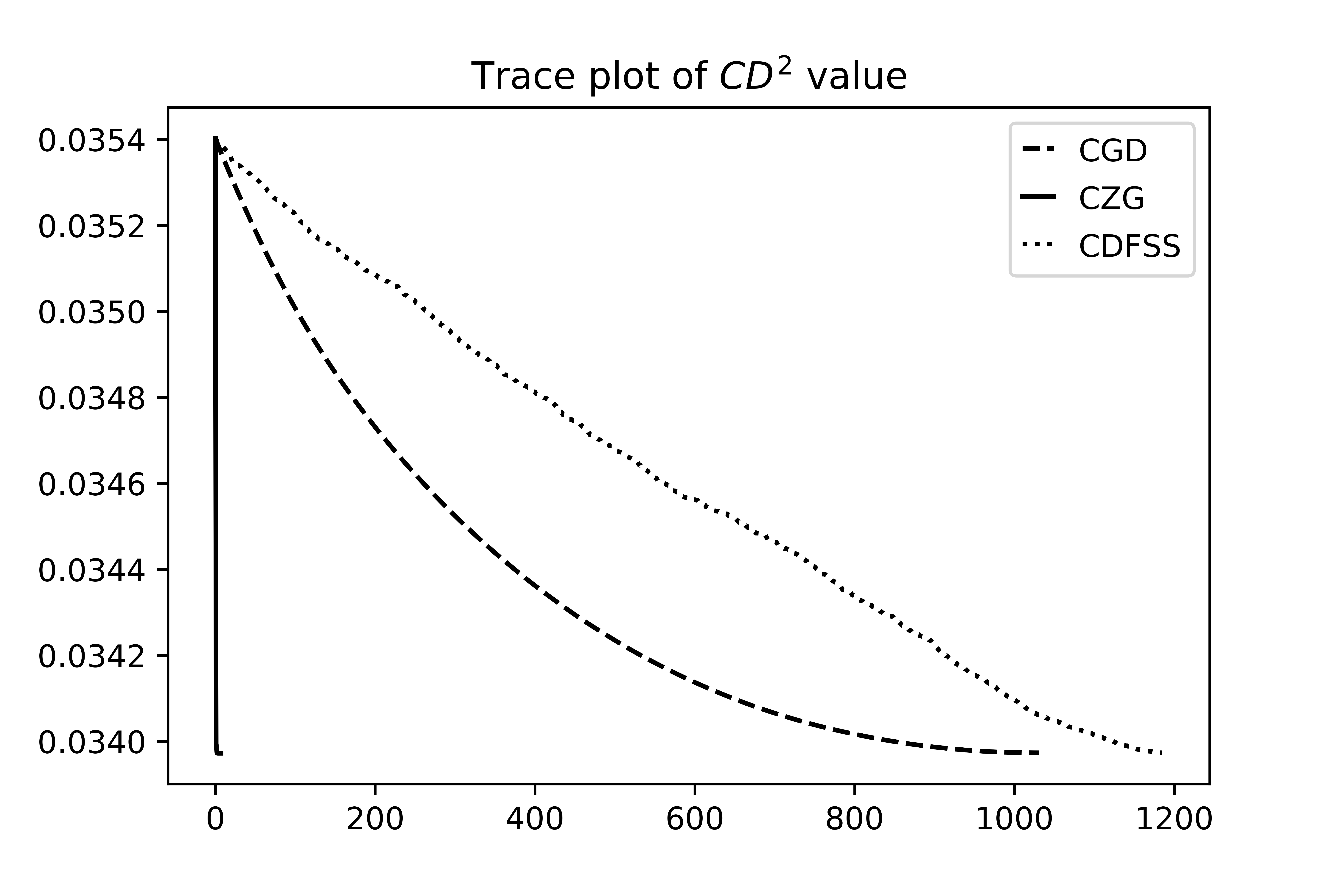
Subsequently, to evaluate the new UDs over continuous domain, we compare the modeling performance of the new designs with the recorded UDs on the website, as well as Latin hypercube sampling in two computer experiments as illustrative instances. The prediction MSE is adopted as evaluation criteria. In this paper, we take Kriging modeling technique to yield the metamodels, that may affect the MSE as well. Nevertheless, it indicates that the new uniform designs are advantaged on modeling in computer experiments. Uniform designs over continuous domain is promising since designs with continuous factors become feasible and in demand with the improvement of computational ability.
6 Acknowledgement
This work was partially supported by the Zhuhai Premier Discipline Grant; Guangdong Natural Science Foundation under Grant No. 2018A0303130231; and BNU-HKBU United International College under Grant R202108. We thank Dr. Peng Heng for his support.
References
- Chipman and Winker, (1995) Chipman, J. S. and Winker, P. (1995). Optimal industrial classification by threshold accepting. Control and Cybernetics, 24:477–494.
- Dueck and Scheuer, (1990) Dueck, G. and Scheuer, T. (1990). Threshold accepting: a general purpose optimization algorithm appearing superior to simulated annealing. Journal of Computational Physics, 90(1):161–175.
- Dueck and Winker, (1992) Dueck, G. and Winker, P. (1992). New concepts and algorithms for portfolio choice. Applied Stochastic Models and Data Analysis, 8(3):159–178.
- Fang, (1980) Fang, K. T. (1980). The uniform design: Application of number-theoretic methods in experimental design. Acta Mathematicae Applicatae Sinica, 3(4):363–372.
- Fang et al., (2017) Fang, K. T., Ke, X., and Elsawah, A. M. (2017). Construction of uniform designs via an adjusted threshold accepting algorithm. Journal of Complexity, 43:28–37.
- Fang et al., (2005) Fang, K. T., Li, R., and Sudjianto, A. (2005). Design and Modeling for Computer Experiments. CRC press.
- Fang et al., (2018) Fang, K. T., Liu, M. Q., Qin, H., and Zhou, Y. D. (2018). Theory and Application of Uniform Experimental Designs. Science Press and Springer.
- Hickernell, (1998) Hickernell, F. (1998). A generalized discrepancy and quadrature error bound. Mathematics of Computation, 67(221):299–322.
- Hua and Wang, (1981) Hua, L. K. and Wang, Y. (1981). Applications of Number Theory to Numerical Analysis. Springer and Science Press.
- Kirkpatrick, (1984) Kirkpatrick, S. (1984). Optimization by simulated annealing: Quantitative studies. Journal of Statistical Physics, 34(5-6):975–986.
- McKay et al., (1979) McKay, M. D., Beckman, R. J., and Conover, W. J. (1979). A comparison of three methods for selecting values of input variables in the analysis of output from a computer code. Technometrics, 21:239–245.
- Ruder, (2016) Ruder, S. (2016). An overview of gradient descent optimization algorithms. arXiv preprint arXiv:1609.04747.
- Shi et al., (2016) Shi, H. J. M., Tu, S., Xu, Y., and Yin, W. (2016). A primer on coordinate descent algorithms. arXiv preprint arXiv:1610.00040.
- Wang and Fang, (1981) Wang, Y. and Fang, K. T. (1981). A note on uniform distribution and experimental design. Kexue Tongbao (Chinese Science Bulletin), (26):485–489.
- Winker, (1994) Winker, P. (1994). The tuning of the threshold accepting heuristic for travelling salesman problems. In Sonderforschungsbereich, volume 178. Universität Konstanz.
- Winker and Fang, (1997) Winker, P. and Fang, K. T. (1997). Application of threshold-accepting to the evaluation of the discrepancy of a set of points. SIAM Journal on Numerical Analysis, 34(5):2028–2042.
- Winker and Fang, (1998) Winker, P. and Fang, K. T. (1998). Optimal u-type designs. In Monte Carlo and Quasi-Monte Carlo Methods 1996, pages 436–448. Springer.
- Wright, (2015) Wright, S. J. (2015). Coordinate descent algorithms. Mathematical Programming, 151(1):3–34.
- Zhou et al., (2013) Zhou, Y. D., Fang, K. T., and Ning, J. H. (2013). Mixture discrepancy for quasi-random point sets. Journal of Complexity, 29(3-4):283–301.