Cosmic chronometers to calibrate the ladders and measure the curvature of the Universe. A model-independent study
Abstract
We use the state-of-the-art data on cosmic chronometers (CCH) and the Pantheon+ compilation of supernovae of Type Ia (SNIa) to test the constancy of the SNIa absolute magnitude, , and the robustness of the cosmological principle (CP) at with a model-agnostic approach. We do so by reconstructing and the curvature parameter using Gaussian Processes. Moreover, we use CCH in combination with data on baryon acoustic oscillations (BAO) from various galaxy surveys (6dFGS, BOSS, eBOSS, WiggleZ, DES Y3) to measure the sound horizon at the baryon-drag epoch, , from each BAO data point and check their consistency. Given the precision allowed by the CCH, we find that , and are fully compatible (at C.L.) with constant values. This justifies our final analyses, in which we put constraints on these constant parameters under the validity of the CP, the metric description of gravity and standard physics in the vicinity of the stellar objects, but otherwise in a model-independent way. If we exclude the SNIa contained in the host galaxies employed by SH0ES, our results read mag, Mpc and , with km/s/Mpc (68% C.L.). These values are independent from the main data sets involved in the tension, namely, the cosmic microwave background and the first two rungs of the cosmic distance ladder. If, instead, we also consider the SNIa in the host galaxies, calibrated with Cepheids, we measure mag, Mpc, and km/s/Mpc.
Keywords:
cosmological parameters – dark energy – distance scale – cosmology: observations.1 Introduction
The absolute distance and time scales in cosmology are set by the Hubble-Lemaître constant, , which also sets the energy scale of the universe’s expansion through the Friedmann equation. Its accurate determination is therefore of utmost importance and has been a long-pursued goal since the very birth of modern (relativistic) cosmology and the idea of an expanding universe, almost one century ago (Hubble 1929). Yet, we still do not have a consensus value for this parameter.
The SH0ES collaboration has measured making use of the distance ladder method. They employ 42 supernovae of Type Ia (SNIa) contained in host galaxies with Cepheids at , i.e. at distances Mpc, to calibrate the absolute magnitude of SNIa, mag. By extending the ladder to the Hubble flow, up to , i.e. Mpc, they obtain km/s/Mpc (Riess et al. 2022). The distance ladder measurement is basically model-independent, since it only relies on the Cosmological Principle (CP) and the assumption that SNIa are good enough standardizable objects, i.e., with a standardized which remains constant from our vicinity to the far end of the Hubble flow.
Cosmic microwave background (CMB) observations, on the other hand, allow us to measure in a model-independent way and very precisely the position of the first acoustic peak of the CMB temperature angular power spectrum or, equivalently, the angle , where is the comoving sound horizon at recombination and the comoving angular diameter distance to the last-scattering surface. However, these two quantities, and , cannot be obtained separately with a model-agnostic method. Pre-recombination physics, which depends of course on the model, fixes and this, in turn, fixes to fulfill the tight constraint on 11 1 The Planck collaboration has measured the CMB acoustic angular scale to precision, (Aghanim et al. 2020).. In the context of the CDM, the fit to the full TT,TE,EE+lensing CMB likelihood from Planck leads to km/s/Mpc (Aghanim et al. 2020). The latter is in tension with SH0ES. This constitutes the well-known tension, the biggest mismatch between the standard model of cosmology and current observations, see (Verde et al. 2019; Perivolaropoulos & Skara 2022b; Abdalla et al. 2022) for dedicated reviews.
The angle is the CMB analogue of the transverse baryon acoustic oscillations (BAO) scale, , which has been measured by several galaxy surveys, with the comoving sound horizon at the baryon-drag epoch and being in this case the characteristic redshift of the survey. As , is also set by the physics in the pre-recombination era. Considering on top of CMB, data from BAO and uncalibrated low- and high-redshift SNIa one gets Mpc and mag in the standard cosmological model (Gómez-Valent 2022b). This value of is again in tension with the one reported by SH0ES, as expected, since their large determination of is induced by the large value of () obtained from the calibration in the host galaxies. A prior on derived from CMB analyses or a precise estimate of the primordial deuterium abundance can be used to calibrate the BAO distances and, consequently, also other low-redshift observables like SNIa, by assuming standard physics before decoupling. This, in turn, can be employed to extract a model-dependent estimate of and is the basis of the so-called inverse distance ladder, which leads again to a small value of the Hubble parameter, very close to the Planck/CDM value (Aubourg et al. 2015; Cuesta et al. 2015; Addison et al. 2018; Abbott et al. 2018; Feeney et al. 2019). We remark that this method only allows for a model-dependent determination of , even when no specific cosmological model is assumed at late times by using, for example, cosmography.
In view of the above discussion, it is clear that the tension can be recast in a tension in the calibrators of the direct and inverse distance ladders, and . These quantities play a crucial role in the Hubble tension (see e.g. Bernal et al. 2016; Aylor et al. 2019; Camarena & Marra 2020a; Camarena & Marra 2020b). It is therefore very important to measure these distance calibrators independently from the CMB and the first rungs of the direct distance ladder, as a means of cross-checking the results obtained with the standard methods described above.
Apart from that, it is also interesting to perform these calibrations in a model-independent way. Many models have been proposed in the last years to alleviate the tension: coupled dark energy models (Pettorino 2013; Gómez-Valent et al. 2020; Agrawal et al. 2021; Archidiacono et al. 2022; Goh et al. 2023), modified gravity (Solà Peracaula et al. 2019; Solà Peracaula et al. 2020; Ballesteros et al. 2020; Braglia et al. 2020; Braglia et al. 2021; Benevento et al. 2022), running vacuum models (Solà Peracaula et al. 2021), early dark energy (Poulin et al. 2019; Niedermann & Sloth 2021; Agrawal et al. 2019; Hill et al. 2020; Gómez-Valent et al. 2021; Gómez-Valent et al. 2022), scenarios with varying atomic constants (Liu et al. 2020a; Sekiguchi & Takahashi 2021; Lee et al. 2023), or models with primordial magnetic fields (Jedamzik & Pogosian 2020). See (Di Valentino et al. 2021a) for a review and a more complete list of references. The vast majority of these proposals introduce some kind of new physics in the last stages of the recombination epoch, triggering shifts in the value of accompanied also by changes at low redshift to keep the good description of the CMB and BAO data. Other authors have suggested an ultra-late time transition in the effective gravitational coupling and hence in at to loosen the tension, (Marra & Perivolaropoulos 2021; Perivolaropoulos 2022; Perivolaropoulos & Skara 2022a). We could use the model-independent estimation of the distance calibrators to assess the viability of these models beyond CDM. Thus, it is clear that calibrating the ladders using independent methods and following model-independent approaches can be very relevant. The results obtained with these alternative methods could be employed to shed some light into the discussion, potentially arbitrating the Hubble tension itself.
In this paper we use the state-of-the-art data on cosmic chronometers (CCH) to calibrate the cosmic ladders and measure the curvature of the universe in a model-independent framework, employing also the Pantheon compilation of SNIa and BAO data from various galaxy surveys (6dFGS, BOSS, eBOSS, WiggleZ, DES Y3). The original idea of this calibration technique was presented in (Sutherland 2012). It was applied for the first time by Heavens et al. 2014 and subsequently employed in several works in the light of new data and different statistical methods, see e.g. (Verde et al. 2017; Haridasu et al. 2018; Dhawan et al. 2021; Gómez-Valent 2022a). It assumes that gravity can be described by a metric theory, together with the CP and the validity of CCH as reliable cosmic clocks, and SNIa and BAO as optimal standard candles and standard rulers, respectively. Here, we reconstruct the shape of from CCH and the one of the apparent magnitude of SNIa with Gaussian Processes (GPs) and use them to test some of these very basic assumptions, which are usually taken for granted in other works. In particular, we reconstruct applying the method proposed by Clarkson et al. 2008 to test the homogeneity property of the universe by checking that this function is compatible with a constant for . See (Cai et al. 2016; Yu & Wang 2016; Liu et al. 2020b) for similar studies along this direction. We also reconstruct the absolute magnitude of SNIa as a function of the redshift, , and check that no evolution is preferred by current data. This analysis is on the lines of the one by Benisty et al. 2023, but we use different data sets, have a better control of the effect of correlations and get rid of double-counting issues. Finally, we perform a consistency test among the BAO data points employed in this paper, and show that according to the low-redshift data sets under consideration, there is no significant statistical tension between them.
All in all, these preliminary tests legitimize the final part of this work, in which we obtain model-independent constraints on and the calibrators and , which are also independent of the main drivers of the Hubble tension. This independent calibration of the ladders is obviously relevant for the discussion of the tension for the reasons already explained. , on the other hand, provides us with information about the early universe and the period of inflation. It is a pivotal parameter. In the context of CDM, the CMB data from Planck prefer a closed universe at C.L. for the Planck TT,TE,EE likelihood, ( C.L.), and at a slightly lower level when also the CMB lensing information is included in the analysis, (Aghanim et al. 2020; Handley 2021; Di Valentino et al. 2019). However, when data on BAO, SNIa, the full-shape galaxy power spectrum or CCH are added on top of CMB, this deviation from spatial flatness disappears (Aghanim et al. 2020; Efstathiou & Gratton 2020; Vagnozzi et al. 2021a; Vagnozzi et al. 2021b). Same conclusions are reached when CMB data from the Atacama Cosmology Telescope are employed alone or in combination with WMAP (Aiola et al. 2020). For a review, we refer the reader to (Di Valentino et al. 2021b). See also the exhaustive work by de Cruz Pérez et al. 2023 for constraints on the curvature in non-flat CDM and its extensions under a large variety of data sets, and (Collett et al. 2019) for a cosmographical measurement of and from SNIa and strong lensing data. In this paper we measure the curvature parameter without assuming any cosmological model.
This manuscript is organized as follows. In Sec. 2 we describe in detail the low- data sets employed throughout the paper, namely CCH, SNIa and BAO. In Sec. 3 we remind the reader what a Gaussian Process is and explain some of its novel and useful technical aspects, e.g. on how to select a kernel applying an objective mathematical criterion. We reconstruct the shape of and , which is important for the subsequent parts of the paper. In Sec. 4 we perform the preliminary tests already mentioned in the previous paragraphs, and in Sec. 5 we calibrate the ladders and measure the curvature of the universe using different data set combinations. We also discuss how our constraints improve if we decrease the uncertainties of the CCH data. In Sec. 6 we finally provide our conclusions.
2 Data
We dedicate this section to describe the low-redshift data sets employed in this study.
2.1 Cosmic chronometers
Massive passively evolving galaxies with old stellar populations and very low star formation rates, i.e. with very little contamination from young components, can be employed as cosmic chronometers using the so-called differential age technique. The idea dates back to the seminal work by Jimenez & Loeb 2002 and is based on the fact that in a Friedmann-Lemaître-Robertson-Walker (FLRW) universe the Hubble function can be written as
| (1) |
with the look-back time differential change with redshift. Passively evolving galaxies formed at high redshift () and over a very short period of time ( Gyr). By comparing two ensembles of galaxies that formed at the same time but with different (close enough) redshifts, it is possible to estimate the derivative using their spectra and a stellar population synthesis (SPS) model. This, in turn, allows us to measure , under the assumption that General Relativity and standard physics hold in the environment of the stars. Apart from that and the CP22 2 The expression (1) might hold even in the presence of cosmic backreaction (Koksbang 2021). Cosmic distances, though, would depart from the FLRW ones, so our analyses of Secs. 4.1, 4.3, and 5 are strictly valid under the assumption of the CP, i.e. if the impact of the backreaction is negligible. See the aforesaid sections for details., the CCH data are free from other cosmological assumptions, what makes these data very suitable to perform model-independent analyses like those we will carry out in this work. In addition, direct measurements of can be employed to calibrate the ladders, since they set the energy scale in the universe. In our study, CCH will play an analogous role to the calibrated Cepheids employed by SH0ES in the direct distance ladder.
We provide the list with the 32 CCH data points employed in this paper in Table 1, together with the original references. They span over the redshift range and constitute the most updated data set on CCH in the literature. In the last years important efforts have been dedicated to build the error budget of the CCH data, see e.g. (Moresco et al. 2020). The full (non-diagonal) covariance matrix of the data is computed as 33 3 https://gitlab.com/mmoresco/CCcovariance:
| (2) |
contains the statistical errors and is diagonal. The systematic uncertainties contained in account for several effects related to the estimate of physical properties of the galaxies, e.g. the stellar metallicity and the possible contamination by a young component, which are uncorrelated for objects at different redshifts. This is not the case for other sources of uncertainty, as they are primarily due to the choice of initial mass function, stellar library, etc., which rely on the common SPS model used to study the evolution of galaxies. See again (Moresco et al. 2020) for a more detailed account of the origin and modeling of systematic errors in the CCH data.
2.2 Supernovae of Type Ia
We make use of the Pantheon compilation of Type Ia supernovae (Scolnic et al. 2022), which includes 1701 light curves of 1550 unique, spectroscopically confirmed SNIa, ranging in redshift from to and coming from 18 different surveys 44 4 https://github.com/PantheonPlusSH0ES/DataRelease. The main changes with respect to the original Pantheon compilation from (Scolnic et al. 2018) are that in Pantheon the sample size (especially at ) and the redshift span are larger, and there has also been an improved treatment of systematic uncertainties in redshifts, peculiar velocities, photometric calibration, and intrinsic-scatter models of SNIa. In particular, we would like to remark that due to some cuts, not all the SNIa contained in Pantheon are found in the improved Pantheon compilation. There are some redshift ranges in which the number of SNIa is smaller, cf. Fig. 1 of (Scolnic et al. 2022).
In this paper we actually use two different SNIa samples. In our main analyses we remove the data points from the SNIa that are contained in the host galaxies of SH0ES (Riess et al. 2022; Brout et al. 2022) in order to obtain results independent of them. The remaining sample contains 1624 data points. In Sec. 5.5 we also use the full Pantheon compilation together with the distances to the host galaxies obtained by SH0ES in the first rungs of the distance ladder to assess their impact in our model-independent measurement of , and .
The SNIa data are given as follows. For each lightcurve we have the apparent magnitude as measured on Earth, , together with the heliocentric and Hubble diagram redshifts, denoted as and (Carr et al. 2022), respectively. If is the standardized absolute magnitude of the SNIa and is the luminosity distance inferred from the measurements for a fixed , we have the following relation,
| (3) |
with
| (4) |
and
| (5) |
where is the curvature density parameter, with for a flat, open and closed universe, respectively. is a constant with units of length that can be interpreted as the current radius of curvature in a closed universe. Using these relations, it is possible to rewrite the expression of the apparent magnitude in the most usual form, only in terms of the redshift ,
| (6) |
This is the apparent magnitude that would be measured in absence of peculiar motions, and is the function we will reconstruct in Sec. 3 to perform the tests of Secs. 4.1 and 4.2. We consider in all our analyses the effect of statistical and systematic uncertainties in the Pantheon+ data through the corresponding non-diagonal covariance matrix.
| Survey | Observable | Measurement | References | |
| 6dFGS+SDSS MGS | 0.122 | [Mpc] | Carter et al. 2018 | |
| WiggleZ | 0.44 | [Mpc] | Kazin et al. 2014 | |
| 0.60 | [Mpc] | |||
| 0.73 | [Mpc] | |||
| BOSS DR12 | 0.32 | Gil-Marín et al. 2017 | ||
| 0.57 | ||||
| DES Y3 | 0.835 | Abbott et al. 2022 | ||
| eBOSS DR16 | 1.48 | Neveux et al. 2020 | ||
| Hou et al. 2020 |
2.3 Baryon Acoustic Oscillations
Acoustic sound waves propagated in the tighly coupled photo-baryon fluid before the decoupling of CMB photons at . They left an imprint in the distribution of galaxies that manifests itself as a peak in the two-point galaxy correlation function, which is located at the maximum distance traveled by the sound wave, i.e. the sound horizon at the baryon drag epoch, . This peak translates into wiggles in the matter power spectrum, its Fourier transform. Several galaxy surveys have measured these features in the last twenty years with increasing degree of precision and spanning different redshift ranges (Cole et al. 2005; Eisenstein et al. 2005). They use as a standard ruler with respect to which they measure cosmological distances at various redshifts. This can be employed to constrain cosmological models in a quite robust way (Sherwin & White 2019; Carter et al. 2020; Bernal et al. 2020; Brieden et al. 2021a; Brieden et al. 2021b). Their constraints are given either in terms of the dilation scale ,
| (7) |
or by splitting (when possible) the angular and radial BAO information, providing data on and separately, with some degree of correlation.
In any Riemannian metric theory of gravity with photons traveling on null geodesics and conservation of the photon number, the Etherington relation (Etherington 1933) holds,
| (8) |
It is very useful, since it can be employed to convert angular diameter distances into luminosity distances, and vice versa. Current low-redshift data does not point to any deviation from this relation (Renzi et al. 2022).
We show the list of BAO data points employed in this work and their corresponding references in Table 2.
3 Gaussian Processes
3.1 The basics
Data-driven reconstructions of cosmological functions subject to minimal model assumptions can be obtained with Gaussian Processes. Based on Bayesian statistics, this machine learning algorithm has become in recent years one of the most widely used model-independent regression techniques in cosmology. It requires the data to be Gaussianly distributed.
A Gaussian Process is a generalization of a multivariate Gaussian, and is defined by the mean function and the covariance matrix , see, e.g., (Rasmussen & Williams 2006). If we denote the collection of the data points that will be employed to train the GP as , being the latter located at points , the covariance matrix takes the following form
| (9) |
where is the covariance matrix of the data and the so-called kernel function. Imagine that we want to reconstruct our function at the locations (). By computing the probability of finding a given realization of the GP under the condition we find that the resulting GP is characterized by the mean function
| (10) |
and the covariance
| (11) |
is the a priori assumed mean of the reconstructed function at . The kernel, which encodes the assumptions on the covariance between points at which we do not have data, plays a central role. There are many possible kernel functions to be employed in a GP, but the simplest choice falls into the category of stationary kernels, which depend only on the distance between the input data points, that is on , and not on their individual values and , being thus invariant to translations in the input space. Although the GP is regarded as a non-parametric method, the kernels introduce some hyperparameters that are typically in charge of controlling the strength of the fluctuations and the correlation length between two separate points. Before the reconstruction, these hyperparameters have to be determined by a proper optimization or marginalization of the GP. These two processes require the maximization or the sampling, respectively, of the likelihood
| (12) |
which is obtained by marginalizing the GP over the points that are not contained in the data set. In many cases, this likelihood is sharply peaked and the optimized result becomes a good approximation (Seikel et al. 2012). This is usually the case when a constant prior mean is employed in the analysis (Hwang et al. 2023). However, strictly speaking, from a Bayesian perspective, getting the full distribution of the hyperparameters is the correct way to proceed. Indeed, if we want to take into account the correlations between the kernel hyperparameters and their uncertainties, we need to abandon the assumption that their distribution is a Dirac delta, see e.g. (Gómez-Valent & Amendola 2018; Hwang et al. 2023). By doing so, the non-zero uncertainties of the hyperparameters can then be propagated to the reconstructed function under study. It is important not to neglect them or, at least, to duly assess their impact on the results. We will do so in Sec. 3.3, together with a study of the impact of the prior mean .
In this work we make use of the public package Gaussian Processes in Python (GaPP) 55 5 https://github.com/carlosandrepaes/GaPP, first developed by Seikel et al. 2012. One of its modules is prepared to perform the Monte Carlo Markov Chain (MCMC) sampling of the kernel hyperparameters. It relies on the public package emcee66 6 https://emcee.readthedocs.io/en/stable/ (Foreman-Mackey et al. 2013), which is a Python implementation of the affine invariant MCMC ensemble sampler by Goodman & Weare 2010.

3.2 A method to select the kernel
We now present a mathematical criterion to select the most suitable kernel among the available ones. We then apply it to the reconstruction of the Hubble function, .
There are six available kernels in the GaPP package. The simplest one is the Squared Exponential, defined as
| (13) |
where and are two hyperparameters, in charge of controlling the correlation length between points and the amplitude of the uncertainties, respectively. The sum of two Squared Exponentials defines the so-called Double Squared Exponential kernel. In GaPP there are also four types of kernels contained in the Matérn family. If we define as the gamma function and as the modified Bessel function of the second kind, the Matérn covariance between two points separated by the distance is given by
| (14) |
where . In the limit we recover the Squared Exponential kernel. The Matérn covariance family is times differentiable in the mean-square sense, i.e. the derivative exists and is finite if . Higher values of translate into wider peaks and smoother reconstructed functions due to the stronger correlation between points. GaPP contains the Matérn kernels with , called Matérn 32, 52, 72 and 92, respectively.
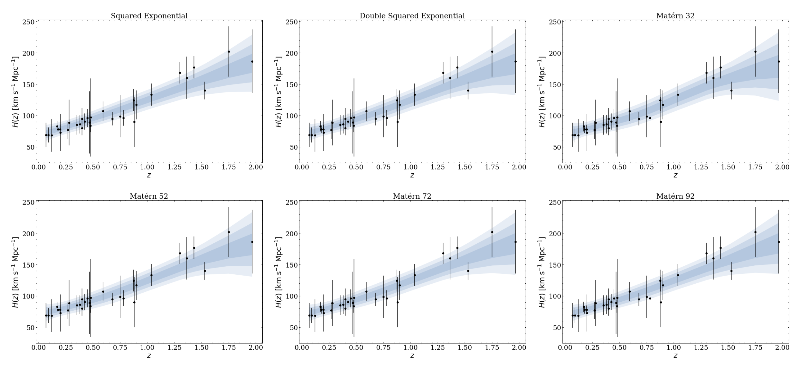
We perform the reconstruction of employing the 32 CCH data points listed in Table 1 with the GP trained with the six aforementioned kernels in the redshift range . We show the results obtained from each kernel in Appendix A, see Fig. 10. Not very significant differences can be appreciated between them with naked eye. To assess the performance of the kernels in the reconstruction of , we proceed as follows. We draw with each kernel GP random realizations, with , accounting for both the covariance of the data points and of the reconstruction. For each realization we compute the statistics, using the following expression,
| Kernels | |
|---|---|
| SE vs DSE | 1.42 |
| SE vs M32 | 0.62 |
| SE vs M52 | 0.72 |
| SE vs M72 | 0.82 |
| SE vs M92 | 0.83 |
| (15) |
where is the covariance matrix of the CCH data and the Latin indices label the redshifts at which we have data. Thus, the realizations of the Hubble function lead to values of . More concretely, in order to penalize the use of additional hyperparameters, we compute the reduced , , with dof being the number of degrees of freedom, i.e. the number of data points minus the number of hyperparameters. We then build a histogram of for each kernel, cf. Fig. 1. Several comments are in order. First, the figure shows that the mean values of lie below and quite far from 1, regardless of the kernel. This might be due to an overestimation of the CCH uncertainties. In Sec. 5.4 we will speculate about this possibility and see how our results change when we allow the CCH data to take smaller errors. Secondly, the kernel Matérn 32 is the one with the lowest mean . However, we need to estimate more quantitatively the relative ability of the kernels to describe the data. Let us consider two kernels and . The probability that the reduced associated to is lower than the one associated to reads,
| (16) |
where in the right-hand side is the ratio of their statistical weights. In practice, if we use a sufficiently large number of realizations, , we can estimate , with being the number of realizations in which and . As we are computing relative weights, we can set e.g. , and compute its relative performance with respect to the Kernels . In the analysis presented in Table 3 stands for the Squared Exponential kernel. It is clear from that table that Matérn 32 is the best-performing kernel regarding the reconstruction of . For completeness, we also check whether this result is sensitive to the ordering of the vectors containing the values of . The results are very stable. Indeed, the ratios differ only by a tiny percentage, which is only due to numerical noise, i.e. it becomes smaller and smaller for increasing values of .


3.3 Reconstruction of and
We reconstruct now the shape of the Hubble function and the apparent magnitude of SNIa using Gaussian Processes and the data described in Secs. 2.1 and 2.2, respectively. As anticipated in the Introduction, the aim of obtaining these model-independent reconstructions is to use them (among other things) to reconstruct first the absolute magnitude of SNIa and the curvature parameter as a function of the redshift, see Sec. 4.
We obtain from CCH following the method and the prescriptions described in Secs. 3.1 and 3.2, i.e. using the Matérn 32 kernel, a zero mean function , and taking into account the full distribution of the hyperparameters and . This, in particular, only has a modest impact on the final reconstruction. The mean in the marginalization procedure differs by 5% at most from the optimized result and the errors are 8% larger. Moreover, we have explicitly checked that we obtain very similar results using . They differ only by . Hence, a full marginalization process that includes also the marginalization over a constant (together with the hyperparameters) leads essentially to the same final reconstructed shape of . In addition, we have also studied what happens if we assume a prior mean based on the CDM prediction, marginalizing also over the parameters and . We find that this introduces very strong model dependencies, basically yielding the same output as in a pure CDM fit. This goes against the philosophy of our work, so we prefer to use a constant mean in our main analyses.
Due to the large covariance matrix of the Pantheon+ compilation, it is very expensive from the computational point of view to perform the marginalization over the hyperparameters and repeat the analysis of Sec. 3.2 for , so we opt to use also in this case the Matérn 32 kernel and the best-fit values obtained from the maximization of the marginalized likelihood Eq. (3.1). Using the binned Pantheon data from (Scolnic et al. 2018), we have checked that the results are not very sensitive to these choices. In addition, we employ the reconstruction of only in some of the tests of Sec. 4. The conclusions of these tests do not depend on these subtleties. To obtain the final constraints on the triad of parameters in Sec. 5 we only make use of the reconstruction of the Hubble rate, which duly incorporates the uncertainties of the hyperparameters.
We show the reconstructed shapes of and in Fig. 2. The extrapolated value of the Hubble parameter reads, km/s/Mpc. For previous reconstructions of the Hubble rate with GPs and CCH see e.g. (Busti et al. 2014; Yu et al. 2018; Gómez-Valent & Amendola 2018; Haridasu et al. 2018; Yang et al. 2023; Renzi & Silvestri 2023), and for previous reconstructions of or the distance modulus from SNIa data see e.g. (Seikel et al. 2012; Cai et al. 2016; Yu & Wang 2016; Yang & Gong 2021; Liang et al. 2022; Renzi & Silvestri 2023).
4 Some tests of the consistency of low- data and the theoretical assumptions behind the standard cosmological model
4.1 Testing the constancy of
In this section we reconstruct the shape of the absolute magnitude of SNIa, , in order to test its constancy throughout the cosmic expansion, in the redshift range . In Sec. 3.3 we have obtained the GPs associated to and . We can reconstruct using formula (2.2). First, we draw realizations (curves) of the Hubble function and the apparent magnitude from their corresponding Gaussian Process. In order to compute the reconstructed shape of the luminosity distance using Eq. (5) we have to employ a prior for the curvature parameter. For this first analysis we fix , while then we will study also other values to assess the impact of this prior on our result. For each realization in the sample, we compute at equispaced knots. We present the reconstructed shape of and its first derivative, , in Fig. 3. From these plots it is evident that the resulting function is fully compatible with a constant at . We have checked that this statement actually holds for a wide range of values of the curvature parameter .
In view of these results, it is natural to estimate the value of the constant from the reconstructed shape of . As we have knots we have distributions of , i.e. one for each knot. These samples are correlated, of course. Assuming that they are Gaussianly distributed, we can construct a probability distribution that takes the following form,


| (17) |
with the normalization constant and the mean value in the -th knot. Let us define now to simplify the notation77 7 Notice that this covariance matrix is different to the one defined in the preceding formula (2).. It is easy to show that Eq. (17) can be rewritten as follows
| (18) |
This means that the distribution of is a Gaussian with mean and deviance
| (19) |
respectively. We estimate the covariance matrix from our sample as follows,
| (20) |
where is the value of the absolute magnitude at the -th knot for each realization .

Applying these formulas, we find mag in the case in which we set . However, this result can only be considered as a first approximation for two reasons: (i) non-Gaussian features, despite being small, can introduce some mild changes, which are not captured by the distribution Eq. (17). However, we have performed a sanity check to verify that the distributions of are Gaussian in very good approximation. At each redshift point where we reconstruct , we build a histogram from its realizations and check that the skewness of each of them is compatible with zero. Hence, the bias introduced by this fact is certainly very small; and (ii) in this calculation all the redshift range is equally weighted, but in reality the data points are not uniformly distributed and this might also have an impact on the estimation of the weighted mean and its uncertainty.


As mentioned before, the shape of is compatible with a constant regardless of the value of chosen to carry out the analysis. Nevertheless, it is important to notice that the value of that constant depends a lot on the prior. In Fig. 4 we show how the constraint on changes with , from values of mag to mag when varies from to . The range of values of explored here is much broader than what is allowed by the CDM constraints from Planck (Aghanim et al. 2020). This has to be consistent with our model-independent approach. As we will see in Sec. 5, large absolute values of the curvature are not excluded by the low-redshift data sets employed in this paper.
The test done in this section demonstrates that with CCH and Pantheon+ data sets, there is no significant statistical preference for the evolution of . However, if we want a robust estimate on the constant value of , we need to constrain simultaneously both and in a joint analysis. This will become even more evident in Sec. 4.2, where we reconstruct .
4.2 Testing the Cosmological Principle
Now, we reconstruct . The result can be employed to test the Cosmological Principle without specifying the energy content of the universe nor the gravity action. Clarkson et al. 2008 proposed to use
| (21) |
with the prime denoting a derivative with respect to the redshift, as a diagnostic of the homogeneity of the universe. This expression is obtained straightforwardly from Eq. (5). Deviations of it from a constant value at any redshift can be considered to be a hint of the breaking of the CP. The function (21) can be reconstructed from measurements of and the luminosity distance. Hence, we can build it from CCH and calibrated SNIa data.
Here, we reconstruct the curvature parameter as a function of , but in an alternative way, which allows us to skip the numerical computation of the derivatives appearing in Eq. (21). It works as follows. We use the GP of to generate samples of the Hubble function. On the other hand, we draw values of from the SH0ES Gaussian prior on the absolute magnitude of SNIa, . With the latter and GP-realizations of we can reconstruct using formula (2.2), and also the angular diameter distance through the Etherington relation (8). We employ all these ingredients to solve Eq. (5) numerically for every redshift and find realizations of . Our results are presented in Fig. 5. The reconstructed function is compatible with a constant, so there is no hint of a violation of the CP. This resonates well with previous results in the literature obtained with older data sets and applying a different methodology, see e.g. (Cai et al. 2016; Yu & Wang 2016; Yang & Gong 2021). We have verified that this finding is again independent of the prior on employed in the analysis, although the constraint we get on the constant value of does depend on it. This is evident from Fig. 5, see also the caption. In Sec. 5 we will provide joint constraints on and in order to get rid of the ambiguity introduced by the subjective choice of the priors.


4.3 Testing the consistency of the BAO data
In this section we test the internal robustness of the BAO data listed in Table 2 in the light of the CCH data. Given the reconstructed expansion rate derived from CCH, we would expect the values of obtained from the various BAO data points to be statistically consistent with each other. Otherwise, this could signal the presence of uncorrected systematic effects in the data.
We apply a method that is completely analogous to the one performed to obtain and in Secs. 4.1 and 4.2, respectively. We use the GP for to generate curves of the Hubble function. From them we can also reconstruct for a fixed curvature parameter (we first consider the case of a flat universe, i.e. ). We compute the angular diameter distances and at the redshifts of the BAO data points. We then draw Gaussian-distributed vectors of BAO data and combine this information to obtain 11 distributions of , i.e. one for each BAO data point.
We present our results in the upper plot of Fig. 6. For those redshifts with two BAO data points (at , cf. Table 2) we use the weighted mean and uncertainty as provided in formula (19) to obtain a single value of . It is clear from that plot that the values of at the various redshift values are consistent with each other. This result still holds (at C.L.) if we allow the universe to take closed or open geometries, as we have explicitly checked by exploring values of .
5 Calibration of the cosmic ladders and measurement of
The analyses carried out in Sec. 4 show no evidence for an evolution of the absolute magnitude of SNIa with redshift nor a departure from homogeneity at large scales. Moreover, we have checked that the BAO data employed in this work are consistent and lead to values of that are fully compatible with each other. Hence, we are legitimated to perform an analysis to jointly constrain the curvature parameter and the calibrators of the distance ladders by treating them simply as constants88 8 We still assume cosmological isotropy, even though this symmetry of the CP has not been tested by us. See (Aluri et al. 2023) for a review of the CP and hints for deviations from it..
We obtain constraints in the planes and using CCH+SNIa (in Sec. 5.1) and CCH+BAO (in Sec. 5.2), respectively, making use of a quite model-independent approach, which is also independent of the data sets that drive the tension. Both, uncalibrated SNIa and BAO, are relative distance indicators. In practice, we use CCH to calibrate the standard candles and the standard rulers. Finally, in Sec. 5.3 we combine the three data sets CCH+SNIa+BAO to constrain the full parameter space . The results of these analyses are shown in Fig. 7 and the derived constraints on the various parameters are presented in Table 4.
In Sec. 5.5 we include the SNIa in the host galaxies and the information of their distances (inferred from calibrated Cepheid variable stars) to assess their impact. In Sec. 5.4 we speculate about the possibility that uncertainties on the CCH have been overestimated. Specifically, we study a case in which CCH uncertainties have been lowered to get a distribution of with a mean equal to one (see Sec. 3.2).

| CCH+SNIa | CCH+BAO | CCH+SNIa+BAO | |
|---|---|---|---|
| M [mag] | |||
| [Mpc] |
5.1 Analysis with CCH+SNIa
We employ the CCH and SNIa data sets to obtain joint constraints in the plane making use of a grid-search method. First, we employ the GP trained with the CCH data to get reconstructed curves of , from which we obtain reconstructions of , i.e. the integral that enters the expression of the luminosity distance Eq. (5). Actually, we only need to keep the values of this function at the redshifts at which we have the SNIa data, so we end up with vectors of values of . Then, we build a rectangular grid in the plane (), with mag and . The size of the steps is not uniform, we use smaller steps in those regions of the plane with a higher probability. This determines the total number of points that make up our grid. At each point of the grid, which is characterized by the values of and , we transform the vectors with into vectors with by virtue of Eq. (5) and, subsequently, in vectors with the apparent magnitude . This enables us to perform a analysis using the SNIa data. For each realizations in the -th knot, we have
| (22) |
where is here the covariance matrix of the SNIa.
To evaluate the behaviour of and and constrain these parameters, we can now use an estimator, , which associates at each knot of the grid a weight proportional to
| (23) |
where the factor accounts for the size of the bins at the -th knot. We use flat priors for and . We can also rewrite the last expression in a slightly different way in order to ease its numerical computation,
| (24) |
with the mean of the in that particular knot. Our estimator reads,
| (25) |
We associate a weight to each knot . The knot at which this quantity is maximum or, equivalently, at which is minimum, is associated to the best-fit values of ().
The two-dimensional probability for the parameters and , , can be easily computed as follows,
| (26) |
where in the denominator we sum over all the knots, and in the numerator we only consider the knot associated to the values and of the parameters and , respectively.
We can also compute the one-dimensional posterior probability for each parameter , , using the analogous expression
| (27) |
where now in the numerator we sum over those knots associated to the value of the parameter .
The one-dimensional posteriors and the confidence regions at 68% and 95% C.L. in all the planes of parameter space are provided in Fig. 7. By evaluating for each parameter the maximum of the probability Eq. (27) and the 68% confidence intervals, we obtain the following results: mag and . The constraint on is similar to the one found by Dhawan et al. 2021 using the Pantheon compilation of SNIa (instead of the most updated Pantheon+) and without considering the correlations between the CCH data nor the data point from (Borghi et al. 2022), . In addition, we also provide a constraint on , which is not reported by Dhawan et al. 2021, since they marginalize their result over it.

5.2 Analysis with CCH+BAO
The same methodology described in Sec. 5.1 can be applied in an analogous way to the plane using the CCH and the BAO data sets. The former is used to calculate vectors with the values of and the angular diameter distance at the BAO redshift points. This information can then be employed to perform a analysis and compute the weights at each point of the grid. In this case the grid ranges are and Mpc.
The resulting constraints read and Mpc. The combination of the CCH data set with the BAO measurements still favors a negative central value for the curvature parameter, although it is compatible with a flat geometry within only . The uncertainty of is smaller than in the analysis with CCH+SNIa. This is clear from the comparison of the green and yellow one-dimensional posteriors of the curvature parameter in Fig. 7.
The posterior of peaks below the preferred Planck/CDM value, Mpc, closer to the region preferred by Early Dark Energy and modified gravity models proposed to alleviate the tension, see e.g. (Poulin et al. 2019; Solà Peracaula et al. 2020). However, this deviation is not statistically significant.
5.3 Joint analysis with CCH+SNIa+BAO
The full parameter space can be now explored to get joint constraints for by taking advantage of the results gathered in Secs. 5.1 and 5.2. We can combine the previous results to get a total as follows,
| (28) |
since the SNIa and BAO data are independent. We use again the expression (27) to obtain the individual constraints for the three parameters. The final results read: mag, and Mpc. As expected, the combination of all the low- data sets employed in this work leads to smaller uncertainties (see Table 4 and Fig. 7), specially in the case of , since this is the only parameter that is constrained from both the CCH+SNIa and CCH+BAO data sets. If we set we find mag and Mpc, which remain extremely close to the main results, but with slightly smaller errors99 9 We take the arithmetic mean of the upper and lower uncertainties to make this comparison..
Our result for the absolute magnitude is independent of the SNIa distance ladder calibration. It is compatible within 1 with , but our method cannot achieve the precision attained by SH0ES (Riess et al. 2022). We study in Sec. 5.5 the impact of considering also the SNIa in the host galaxies and their distances. Our value of is also in agreement with the one in (Gómez-Valent 2022a), obtained using a different method based on the index of inconsistency by Lin & Ishak 2017, the Pantheon data set and less CCH data points, but still making use of the combination CCH+BAO+SNIa. We find a 1-compatibility also with the CDM result mag (Gómez-Valent 2022b), although we remark again that our results have been obtained in a model-independent way.
Our measurement of points very mildly to a closed universe, being compatible with the flatness assumption within only . In contrast to the previous work (Gómez-Valent 2022a), which reports , here we do not make use of any cosmological prior inspired by the Planck/CDM results. The latter would dominate the final constraint on the curvature parameter over the low- data sets, something that we wanted to avoid here. The uncertainty of is much larger than the one obtained in model-dependent analyses like the one by Aghanim et al. 2020 or Vagnozzi et al. 2021b. The latter obtain in the context of the non-flat CDM by combining the CMB data from Planck with CCH.
The calibration of the standard ruler with CCH+SNIa+BAO leads to a value which is smaller than the CDM value preferred by Planck (Aghanim et al. 2020), similar to the one obtained from the CCH+BAO analysis, and again peaks at values more in accordance with theoretical scenarios that alleviate the Hubble tension. Our value of the sound horizon at the drag epoch is also compatible with other model-independent analyses, as those by Haridasu et al. 2018, Mpc, and Gómez-Valent 2022a, Mpc.
We also measure employing as a prior our CCH+SNIa+BAO constraint on and the apparent magnitudes of the SNIa in the Hubble flow (). We make use of the cosmographical expansion
| (29) |
Curvature corrections are of third order in and, hence, we can neglect them in this analysis. We obtain km/s/Mpc, with an uncertainty that is roughly a factor smaller than the one obtained using only CCH, see Sec. 3.3. As a byproduct, we also constrain the deceleration parameter . This result is fully compatible with the model-independent measurements extracted from CCH+SNIa+BAO (Haridasu et al. 2018; Gómez-Valent 2019), but with an uncertainty a factor two larger, since here is fixed only by the SNIa in the Hubble flow.
Our results are independent of the direct and inverse distance ladders, quite model-independent and robust under the use of alternative GP kernels (cf. Appendix B). This is interesting per se. However, they cannot arbitrate the tension yet. The low-redshift data sets under consideration give still room to new physics both in the pre- and post-recombination eras.
| CCH+SNIa_host | CCH+BAO | CCH+SNIa_host+BAO | |
|---|---|---|---|
| M [mag] | |||
| [Mpc] |
5.4 Considering smaller uncertainties in the CCH data
The GPs kernel performance test done in Sec. 3.2 shows that the mean values of the reduced chi-square, Eq. (15), associated to the reconstruction of with the CCH data points listed in Table 1 are all much smaller than 1 (see also Fig. 1). This result is not expected to be due to an overfitting of the GP, since similar values of the are also found in fitting analyses with a simple straight line or a parabola, cf. Table 5 of (Gómez-Valent & Amendola 2018). As already mentioned, the small values of could instead be a hint of an overestimation of the errors in the covariance matrix of the CCH data, . In this section, we want to explore this possibility by studying how the results in the analyses of Secs. 5.1-5.3 change if we allow for smaller uncertainties in . With this aim we build the new CCH covariance matrix , with a positive factor. This is equivalent to decrease all the individual CCH uncertainties by a common factor , while leaving the previous correlation coefficients intact. For this purpose, we first repeat the test of Sec. 3.2 with the Matérn 32 kernel, but increasing the values of until the mean of the corresponding reduced chi-squared equals one, i.e. until . We find that this happens when the CCH uncertainties decrease by a factor . We denote the resulting CCH data set with the new covariance matrix simply as CCHnew to distinguish it from the original one (CCH). We can now repeat the analyses of Secs. 5.1-5.3 with CCHnew to study the impact of this change on the data uncertainties, bearing in mind that this is only a first (naive) attempt to estimate the impact of a possible overestimation of the uncertainties of the CCH data1010 10 A more refined analysis would probably require a better understanding of the systematics in the data and/or the application of an improved statistical method, on the lines of what was done by Hobson et al. 2002.. This leads to the following CCHnew+SNIa+BAO constraints: mag, and Mpc. The uncertainties of and decrease by a 30%-40% with respect to those found in the CCH+SNIa+BAO analysis (see also Fig. 7). We do not find, however, the same decrease in the uncertainty of . The reason is simple. Let us focus on the combination CCHnew+SNIa. The low-redshift data at basically constraints and is insensitive to the curvature parameter. At larger redshifts, though, we can get constraints on , which depend on the reconstruction of the ratio , see formula (5). The point is that the correlation coefficients employed in the new CCH data set are exactly the same as those used in the original analysis, what makes the reconstructed shape of to remain the same. This fact, in turn, explains why we find the same constraint on as well.


5.5 Inclusion of the SNIa in the host galaxies and their distances
In our main analyses of Secs. 5.1-5.3, and also in Sec. 5.4, we have excluded the SNIa located in the Cepheid host galaxies, i.e. those employed by SH0ES to calibrate the SNIa in the second rung of the cosmic distance ladder (Riess et al. 2022; Scolnic et al. 2022). We do so to obtain results that are independent of the main drivers of the Hubble tension. Nevertheless, we may ask ourselves which is the impact of considering this additional information, which actually is included in the full Pantheon+ compilation. We call this SNIa data set SNIa_host, in short, and follow the same procedure applied in Secs. 5.1-5.3. The results of this analysis are shown in Fig. 8 and listed in Table 5. The output from the analysis with CCH+BAO is not sensitive to the changes in the SNIa data set, for obvious reasons. As expected, the constraints on are fully dominated by the calibration of the SNIa at the host galaxies. In particular, for the CCH+SNIa_host+BAO analysis we obtain: mag, and Mpc, with km/s/Mpc. No important differences are found in the curvature parameter and with respect to the results presented in Sec. 5.3.
6 Conclusions
In this paper we have first reconstructed the absolute magnitude of SNIa and the curvature of the universe as a function of the redshift up to making use of Gaussian Processes and data on cosmic chronometers and the Pantheon+ compilation of supernovae of Type Ia. We have found that these low-redshift data sets do not point to a time evolution of the SNIa intrinsic luminosity nor a breaking of the homogeneity of the universe at large scales. Both, and are compatible at C.L. with a constant. In addition, we have also tested the consistency of the BAO data from the galaxy surveys 6dFGS, BOSS, eBOSS, WiggleZ and DES Y3, by checking that they are all compatible with a common value of , at least under the precision offered by the CCH data. Motivated by these results, we have then constrained with CCH, SNIa and BAO the constant values of and the calibrators of the direct and inverse distance ladders, and . We have done so by applying a quite model-independent method, which is also independent from the first rungs of the cosmic distance ladder employed by SH0ES and the CMB data from Planck, i.e. from the main data sets involved in the Hubble tension. This is in contrast to other results obtained in the context of the CDM, see e.g. (Aghanim et al. 2020; Handley 2021; Di Valentino et al. 2019; Gómez-Valent 2022b). We obtain: , mag and Mpc. We have checked that the inclusion of the SNIa in the host galaxies and their distances only affects the value of , making its central value and uncertainties to be very close to those measured by SH0ES.
Our results improve previous constraints in the literature obtained also with Gaussian Processes but with slightly different data sets and methodologies. For instance, Benisty et al. 2023 obtained mag from data on BAO and SNIa together with a Planck prior for . We, instead, have measured with an uncertainty three times smaller. In addition, we have extracted joint and model-independent constraints for and as well, with a more refined BAO data set, which is free from double-counting issues and incorporates the effect of correlations. Our determination of is more precise than the one carried out by Dhawan et al. 2021, , thanks mainly to the use of BAO data on top of the CCH and the Pantheon+ compilation of SNIa. The same level of improvement is also obtained compared to the cosmographical analysis of SNIa and strong lensing data by Collett et al. 2019, who reported . The present work also improves the analysis of (Gómez-Valent 2022a), since here we have not used any external prior for the curvature parameter and have employed the SNIa contained in the Pantheon+ compilation, instead of those of Pantheon. However, the uncertainties that we have found are still one order of magnitude larger compared to the model-dependent determinations by Planck (Aghanim et al. 2020). As discussed by Dhawan et al. 2021, this could change in the next years, when e.g. SNIa data from the Vera C. Rubin Observatory’s Legacy Survey of Space and Time (LSST, Abell et al. 2009; Ivezić et al. 2019) and BAO data from Euclid (Laureijs et al. 2011) and the Dark Energy Spectroscopic Instrument (DESI, Aghamousa et al. 2016) become available. This will not only decrease the uncertainties of the curvature parameter through the model-independent analyses of standard candles and large-scale structure data (Amendola & Quartin 2021; Amendola et al. 2022), but also improve the constraints we get for the calibrators and , which is obviously important for the discussion of the tension. As shown in Fig. 9, in the light of the current low-redshift data our method does not let us arbitrate the tension yet (we obtain km/s/Mpc with CCH+SNIa+BAO), but we might be able to do so with the advent of the aforementioned upcoming telescopes and surveys. We have seen in Sec. 5.4 that a decrease by a factor 3/2 of the uncertainties of the CCH data produces a decrease of the uncertainties of the calibrators. Thus, an improvement in the CCH data, either in terms of quality or quantity, can also have a non-negligible impact on the outcome of this method. Euclid, for instance, is expected to provide up to a few thousands passively evolving galaxies at , increasing by 2 orders of magnitude the currently available statistics (Moresco et al. 2022).
The method we propose will then find interesting applications in the future, when all these new data become a reality. It will serve as both a discriminator of models beyond the CDM and an independent means of testing the calibration of the direct and inverse cosmic distance ladders.
Appendix A GP-reconstruction of with different kernels
In Sec. 3.2 we have explained a method to select in an objective way a GP-kernel among a group of them given a collection of data points. Here, we just show in Fig. 10 the reconstructed shapes of the Hubble function obtained from six different kernels, namely: Squared Exponential, Double Squared Exponential, Matérn 32, Matérn 52, Matérn 72 and Matérn 92. As already discussed, the differences are not important. This resonates well with the results reported in Table 3 and the conclusions reached in Sec. 3.2.
Appendix B Results with the Gaussian kernel
In this appendix we briefly study the robustness of the results presented in Secs. 5.1-5.3 under the choice of a different GP kernel. To do so, we adopt the Gaussian kernel, which is defined by Eq. (13). It is the smoothest kernel within the Matérn family. It is infinitely differentiable, and so is also the reconstructed function obtained from the GP, see Sec. 3.2 for details. Using the Gaussian kernel instead of Matérn 32 we find the following results with the compilation of data CCH+SNIa+BAO: mag, and Mpc. By comparing these results to those provided in Table 4 we see that they are stable under the choice of the kernel. The shift in the central value of is equal to the bin size of the grid, whereas we find a decrease in the error bars of and a in , and completely compatible results also for the central values of these parameters. In our main analysis we opt, though, to employ Matérn 32, since this is the kernel that leads to the most conservative results, cf. again Sec. 3.2.
Acknowledgments
AGV is funded by the Istituto Nazionale di Fisica Nucleare (INFN) through the project of the InDark INFN Special Initiative: “Dark Energy and Modified Gravity Models in the light of Low-Redshift Observations” (n. 22425/2020). He also acknowledges the participation in the COST Action CA21136 “Addressing observational tensions in cosmology with systematics and fundamental physics” (CosmoVerse). The authors acknowledge support by the INFN project “InDark”. MM is also supported by the ASI/LiteBIRD grant n. 2020-9-HH.0 and by the Fondazione ICSC, Spoke 3 Astrophysics and Cosmos Observations, National Recovery and Resilience Plan (Piano Nazionale di Ripresa e Resilienza, PNRR) Project ID CN_00000013 "Italian Research Center on High-Performance Computing, Big Data and Quantum Computing" funded by MUR Missione 4 Componente 2 Investimento 1.4: Potenziamento strutture di ricerca e creazione di "campioni nazionali di R&S (M4C2-19 )" - Next Generation EU (NGEU).
Data availability
The data employed in this article are publicly available (see Sec. 2 and references therein) and our codes will be shared on reasonable request.
References
- Abbott et al. (2018) Abbott T. M. C., et al., 2018, Mon. Not. Roy. Astron. Soc., 480, 3879
- Abbott et al. (2022) Abbott T., et al., 2022, Physical Review D, 105
- Abdalla et al. (2022) Abdalla E., et al., 2022, JHEAp, 34, 49
- Abell et al. (2009) Abell P. A., et al., 2009, arXiv:0912.0201
- Addison et al. (2018) Addison G. E., Watts D. J., Bennett C. L., Halpern M., Hinshaw G., Weiland J. L., 2018, Astrophys. J., 853, 119
- Aghamousa et al. (2016) Aghamousa A., et al., 2016, arXiv:1611.00036
- Aghanim et al. (2020) Aghanim N., et al., 2020, Astron. Astrophys., 641, A6
- Agrawal et al. (2019) Agrawal P., Cyr-Racine F.-Y., Pinner D., Randall L., 2019, arXiv:1904.01016
- Agrawal et al. (2021) Agrawal P., Obied G., Vafa C., 2021, Phys. Rev. D, 103, 043523
- Aiola et al. (2020) Aiola S., et al., 2020, JCAP, 12, 047
- Aluri et al. (2023) Aluri P. K., et al., 2023, Class. Quant. Grav., 40, 094001
- Amendola & Quartin (2021) Amendola L., Quartin M., 2021, Mon. Not. Roy. Astron. Soc., 504, 3884
- Amendola et al. (2022) Amendola L., Pietroni M., Quartin M., 2022, JCAP, 11, 023
- Archidiacono et al. (2022) Archidiacono M., Castorina E., Redigolo D., Salvioni E., 2022, JCAP, 10, 074
- Aubourg et al. (2015) Aubourg E., et al., 2015, Phys. Rev. D, 92, 123516
- Aylor et al. (2019) Aylor K., Joy M., Knox L., Millea M., Raghunathan S., Wu W. L. K., 2019, Astrophys. J., 874, 4
- Ballesteros et al. (2020) Ballesteros G., Notari A., Rompineve F., 2020, JCAP, 11, 024
- Benevento et al. (2022) Benevento G., Kable J. A., Addison G. E., Bennett C. L., 2022, Astrophys. J., 935, 156
- Benisty et al. (2023) Benisty D., Mifsud J., Levi Said J., Staicova D., 2023, Phys. Dark Univ., 39, 101160
- Bernal et al. (2016) Bernal J. L., Verde L., Riess A. G., 2016, JCAP, 10, 019
- Bernal et al. (2020) Bernal J. L., Smith T. L., Boddy K. K., Kamionkowski M., 2020, Phys. Rev. D, 102, 123515
- Borghi et al. (2022) Borghi N., Moresco M., Cimatti A., 2022, Astrophys. J. Lett., 928, L4
- Braglia et al. (2020) Braglia M., Ballardini M., Emond W. T., Finelli F., Gumrukcuoglu A. E., Koyama K., Paoletti D., 2020, Phys. Rev. D, 102, 023529
- Braglia et al. (2021) Braglia M., Ballardini M., Finelli F., Koyama K., 2021, Phys. Rev. D, 103, 043528
- Brieden et al. (2021a) Brieden S., Gil-Marín H., Verde L., 2021a, JCAP, 12, 054
- Brieden et al. (2021b) Brieden S., Gil-Marín H., Verde L., 2021b, Phys. Rev. D, 104, L121301
- Brout et al. (2022) Brout D., et al., 2022, Astrophys. J., 938, 110
- Bruzual & Charlot (2003) Bruzual G., Charlot S., 2003, Mon. Not. Roy. Astron. Soc., 344, 1000
- Busti et al. (2014) Busti V. C., Clarkson C., Seikel M., 2014, Mon. Not. Roy. Astron. Soc., 441, 11
- Cai et al. (2016) Cai R.-G., Guo Z.-K., Yang T., 2016, Phys. Rev. D, 93, 043517
- Camarena & Marra (2020a) Camarena D., Marra V., 2020a, Phys. Rev. Res., 2, 013028
- Camarena & Marra (2020b) Camarena D., Marra V., 2020b, Mon. Not. Roy. Astron. Soc., 495, 2630
- Carr et al. (2022) Carr A., Davis T. M., Scolnic D., Scolnic D., Said K., Brout D., Peterson E. R., Kessler R., 2022, Publ. Astron. Soc. Austral., 39, e046
- Carter et al. (2018) Carter P., Beutler F., Percival W. J., Blake C., Koda J., Ross A. J., 2018, Monthly Notices of the Royal Astronomical Society, 481, 2371
- Carter et al. (2020) Carter P., Beutler F., Percival W. J., DeRose J., Wechsler R. H., Zhao C., 2020, Mon. Not. Roy. Astron. Soc., 494, 2076
- Clarkson et al. (2008) Clarkson C., Bassett B., Lu T. H.-C., 2008, Phys. Rev. Lett., 101, 011301
- Cole et al. (2005) Cole S., et al., 2005, Mon. Not. Roy. Astron. Soc., 362, 505
- Collett et al. (2019) Collett T., Montanari F., Rasanen S., 2019, Phys. Rev. Lett., 123, 231101
- Cuesta et al. (2015) Cuesta A. J., Verde L., Riess A., Jimenez R., 2015, Mon. Not. Roy. Astron. Soc., 448, 3463
- Dhawan et al. (2021) Dhawan S., Alsing J., Vagnozzi S., 2021, Mon. Not. Roy. Astron. Soc., 506, L1
- Di Valentino et al. (2019) Di Valentino E., Melchiorri A., Silk J., 2019, Nature Astron., 4, 196
- Di Valentino et al. (2021a) Di Valentino E., et al., 2021a, Class. Quant. Grav., 38, 153001
- Di Valentino et al. (2021b) Di Valentino E., et al., 2021b, Astropart. Phys., 131, 102607
- Efstathiou & Gratton (2020) Efstathiou G., Gratton S., 2020, Mon. Not. Roy. Astron. Soc., 496, L91
- Eisenstein et al. (2005) Eisenstein D. J., et al., 2005, Astrophys. J., 633, 560
- Etherington (1933) Etherington I., 1933, Philos. Mag., 15, 761
- Feeney et al. (2019) Feeney S. M., Peiris H. V., Williamson A. R., Nissanke S. M., Mortlock D. J., Alsing J., Scolnic D., 2019, Phys. Rev. Lett., 122, 061105
- Foreman-Mackey et al. (2013) Foreman-Mackey D., Hogg D. W., Lang D., Goodman J., 2013, Publications of the Astronomical Society of the Pacific, 125, 306
- Gil-Marín et al. (2017) Gil-Marín H., Percival W. J., Verde L., Brownstein J. R., Chuang C.-H., Kitaura F.-S., Rodríguez-Torres S. A., Olmstead M. D., 2017, Monthly Notices of the Royal Astronomical Society, 465, 1757
- Goh et al. (2023) Goh L. W. K., Gómez-Valent A., Pettorino V., Kilbinger M., 2023, Phys. Rev. D, 107, 083503
- Gómez-Valent (2019) Gómez-Valent A., 2019, JCAP, 05, 026
- Gómez-Valent (2022a) Gómez-Valent A., 2022a, Phys. Rev. D, 105, 043528
- Gómez-Valent (2022b) Gómez-Valent A., 2022b, Phys. Rev. D, 106, 063506
- Gómez-Valent & Amendola (2018) Gómez-Valent A., Amendola L., 2018, JCAP, 04, 051
- Gómez-Valent et al. (2020) Gómez-Valent A., Pettorino V., Amendola L., 2020, Phys. Rev. D, 101, 123513
- Gómez-Valent et al. (2021) Gómez-Valent A., Zheng Z., Amendola L., Pettorino V., Wetterich C., 2021, Phys. Rev. D, 104, 083536
- Gómez-Valent et al. (2022) Gómez-Valent A., Zheng Z., Amendola L., Wetterich C., Pettorino V., 2022, Phys. Rev. D, 106, 103522
- Goodman & Weare (2010) Goodman J., Weare J., 2010, Communications in Applied Mathematics and Computational Science, 5, 65
- Handley (2021) Handley W., 2021, Phys. Rev. D, 103, L041301
- Haridasu et al. (2018) Haridasu B. S., Luković V. V., Moresco M., Vittorio N., 2018, JCAP, 10, 015
- Heavens et al. (2014) Heavens A., Jimenez R., Verde L., 2014, Phys. Rev. Lett., 113, 241302
- Hill et al. (2020) Hill J. C., McDonough E., Toomey M. W., Alexander S., 2020, Phys. Rev. D, 102, 043507
- Hobson et al. (2002) Hobson M. P., Bridle S. L., Lahav O., 2002, Mon. Not. Roy. Astron. Soc., 335, 377
- Hou et al. (2020) Hou J., et al., 2020, Monthly Notices of the Royal Astronomical Society, 500, 1201
- Hubble (1929) Hubble E., 1929, Proc. Nat. Acad. Sci., 15, 168
- Hwang et al. (2023) Hwang S.-g., L’Huillier B., Keeley R. E., Jee M. J., Shafieloo A., 2023, JCAP, 02, 014
- Ivezić et al. (2019) Ivezić v., et al., 2019, Astrophys. J., 873, 111
- Jedamzik & Pogosian (2020) Jedamzik K., Pogosian L., 2020, Phys. Rev. Lett., 125, 181302
- Jimenez & Loeb (2002) Jimenez R., Loeb A., 2002, Astrophys. J., 573, 37
- Jimenez et al. (2003) Jimenez R., Verde L., Treu T., Stern D., 2003, Astrophys. J., 593, 622
- Kazin et al. (2014) Kazin E. A., et al., 2014, Monthly Notices of the Royal Astronomical Society, 441, 3524
- Koksbang (2021) Koksbang S. M., 2021, Phys. Rev. Lett., 126, 231101
- Laureijs et al. (2011) Laureijs R., et al., 2011, arXiv:1110.3193
- Lee et al. (2023) Lee N., Ali-Haïmoud Y., Schöneberg N., Poulin V., 2023, Phys. Rev. Lett., 130, 161003
- Liang et al. (2022) Liang N., Li Z., Xie X., Wu P., 2022, Astrophys. J., 941, 84
- Lin & Ishak (2017) Lin W., Ishak M., 2017, Phys. Rev. D, 96, 023532
- Liu et al. (2020a) Liu M., Huang Z., Luo X., Miao H., Singh N. K., Huang L., 2020a, Sci. China Phys. Mech. Astron., 63, 290405
- Liu et al. (2020b) Liu Y., Cao S., Liu T., Li X., Geng S., Lian Y., Guo W., 2020b, Astrophys. J., 901, 129
- Maraston & Stromback (2011) Maraston C., Stromback G., 2011, Mon. Not. Roy. Astron. Soc., 418, 2785
- Marra & Perivolaropoulos (2021) Marra V., Perivolaropoulos L., 2021, Phys. Rev. D, 104, L021303
- Moresco (2015) Moresco M., 2015, Mon. Not. Roy. Astron. Soc., 450, L16
- Moresco et al. (2012) Moresco M., et al., 2012, JCAP, 08, 006
- Moresco et al. (2016) Moresco M., et al., 2016, JCAP, 05, 014
- Moresco et al. (2020) Moresco M., Jimenez R., Verde L., Cimatti A., Pozzetti L., 2020, Astrophys. J., 898, 82
- Moresco et al. (2022) Moresco M., et al., 2022, Living Rev. Rel., 25, 6
- Neveux et al. (2020) Neveux R., et al., 2020, Monthly Notices of the Royal Astronomical Society, 499, 210
- Niedermann & Sloth (2021) Niedermann F., Sloth M. S., 2021, Phys. Rev. D, 103, L041303
- Perivolaropoulos (2022) Perivolaropoulos L., 2022, Universe, 8, 263
- Perivolaropoulos & Skara (2022a) Perivolaropoulos L., Skara F., 2022a, Universe, 8, 502
- Perivolaropoulos & Skara (2022b) Perivolaropoulos L., Skara F., 2022b, New Astron. Rev., 95, 101659
- Pettorino (2013) Pettorino V., 2013, Phys. Rev. D, 88, 063519
- Poulin et al. (2019) Poulin V., Smith T. L., Karwal T., Kamionkowski M., 2019, Phys. Rev. Lett., 122, 221301
- Rasmussen & Williams (2006) Rasmussen C. E., Williams C. K. I., 2006, Gaussian Processes for Machine Learning. MIT Press
- Ratsimbazafy et al. (2017) Ratsimbazafy A., Loubser S., Crawford S., Cress C., Bassett B., Nichol R., Väisänen P., 2017, Mon. Not. Roy. Astron. Soc., 467, 3239
- Renzi & Silvestri (2023) Renzi F., Silvestri A., 2023, Phys. Rev. D, 107, 023520
- Renzi et al. (2022) Renzi F., Hogg N. B., Giarè W., 2022, Mon. Not. Roy. Astron. Soc., 513, 4004
- Riess et al. (2022) Riess A. G., et al., 2022, Astrophys. J. Lett., 934, L7
- Scolnic et al. (2018) Scolnic D. M., et al., 2018, Astrophys. J., 859, 101
- Scolnic et al. (2022) Scolnic D., et al., 2022, Astrophys. J., 938, 113
- Seikel et al. (2012) Seikel M., Clarkson C., Smith M., 2012, JCAP, 06, 036
- Sekiguchi & Takahashi (2021) Sekiguchi T., Takahashi T., 2021, Phys. Rev. D, 103, 083507
- Sherwin & White (2019) Sherwin B. D., White M., 2019, JCAP, 02, 027
- Simon et al. (2005) Simon J., Verde L., Jimenez R., 2005, Phys. Rev. D, 71, 123001
- Solà Peracaula et al. (2019) Solà Peracaula J., Gómez-Valent A., de Cruz Pérez J., Moreno-Pulido C., 2019, Astrophys. J. Lett., 886, L6
- Solà Peracaula et al. (2020) Solà Peracaula J., Gómez-Valent A., de Cruz Pérez J., Moreno-Pulido C., 2020, Class. Quant. Grav., 37, 245003
- Solà Peracaula et al. (2021) Solà Peracaula J., Gómez-Valent A., de Cruz Pérez J., Moreno-Pulido C., 2021, EPL, 134, 19001
- Stern et al. (2010) Stern D., Jimenez R., Verde L., Kamionkowski M., Stanford S., 2010, JCAP, 02, 008
- Sutherland (2012) Sutherland W., 2012, Mon. Not. Roy. Astron. Soc., 426, 1280
- Vagnozzi et al. (2021a) Vagnozzi S., Di Valentino E., Gariazzo S., Melchiorri A., Mena O., Silk J., 2021a, Phys. Dark Univ., 33, 100851
- Vagnozzi et al. (2021b) Vagnozzi S., Loeb A., Moresco M., 2021b, Astrophys. J., 908, 84
- Verde et al. (2017) Verde L., Bernal J. L., Heavens A. F., Jimenez R., 2017, Mon. Not. Roy. Astron. Soc., 467, 731
- Verde et al. (2019) Verde L., Treu T., Riess A. G., 2019, Nature Astron., 3, 891
- Yang & Gong (2021) Yang Y., Gong Y., 2021, Mon. Not. Roy. Astron. Soc., 504, 3092
- Yang et al. (2023) Yang Y., Lu X., Qian L., Cao S., 2023, Mon. Not. Roy. Astron. Soc., 519, 4938
- Yu & Wang (2016) Yu H., Wang F., 2016, Astrophys. J., 828, 85
- Yu et al. (2018) Yu H., Ratra B., Wang F.-Y., 2018, Astrophys. J., 856, 3
- Zhang et al. (2014) Zhang C., Zhang H., Yuan S., Zhang T.-J., Sun Y.-C., 2014, Res. Astron. Astrophys., 14, 1221
- de Cruz Pérez et al. (2023) de Cruz Pérez J., Park C.-G., Ratra B., 2023, Phys. Rev. D, 107, 063522