2022
Federated learning has become a popular tool in the big data era nowadays. It trains a centralized model based on data from different clients while keeping data decentralized. In this paper, we propose a federated sparse sliced inverse regression algorithm for the first time. Our method can simultaneously estimate the central dimension reduction subspace and perform variable selection in a federated setting. We transform this federated high-dimensional sparse sliced inverse regression problem into a convex optimization problem by constructing the covariance matrix safely and losslessly. We then use a linearized alternating direction method of multipliers algorithm to estimate the central subspace. We also give approaches of Bayesian information criterion and hold-out validation to ascertain the dimension of the central subspace and the hyper-parameter of the algorithm. We establish an upper bound of the statistical error rate of our estimator under the heterogeneous setting. We demonstrate the effectiveness of our method through simulations and real world applications.
MSC Classification]62H12, 62R07
Federated Sufficient Dimension Reduction Through High-Dimensional Sparse Sliced Inverse Regression
keywords
Federated learning, Sliced inverse regression, Sufficient dimension reduction, Variable selectionpacs
[1 Introduction
Federated learning is a distributed machine learning paradigm that collaboratively trains a model with data on many clients. Unlike traditional distributed machine learning methods, which partition data into different clients to improve the efficiency of the learning algorithm, the goal of federated learning is to solve the learning problem without requiring the clients to reveal too much local information. With the increasing demand for data security and privacy protection, federated learning has received significant attention in both industry and academia. For example, banks want to collaboratively train a credit card scoring model without disclosing information about their customers, or hospitals want to carry out researches on a rare disease with each other due to the small number of sample cases, but they can’t expose their patients’ identity. For more on the progress of federated learning, see Kairouz2019; Yang2020FL.
The term federated learning was introduced by McMahan et al. McMahan2016, they also proposed the Federated Averaging (FedAvg) algorithm. FedAvg composes multiple rounds of local stochastic gradient descent updates and server-side averaging aggregation to train a centralized model. FedAvg and its variants such as FedProx (LiTian2018FedProx), SCAFFOLD (Mohri2019SCAFFOLD) and FedAc (yuan2020fedac) mainly focus on deep neural networks, while federated adaptations of traditional machine learning methods are rarely studied. Especially in the area of dimension reduction and variable selection, few researches have appeared under federated learning settings. Grammenos et al. grammenos2020fpca proposed the federated principal component analysis (FedPCA) to reduce the dimensionality of the data. Chai et al. chai2021fedsvd offered masking-based federated singular vector decomposition (FedSVD) method, which can also perform dimension reduction by picking the right singular vectors with the largest singular values as the projection matrix. However, principal component analysis is an unsupervised learning method that doesn’t take into account the relationship between the responses and covariates. Federated learning mainly applies to regression or classification problems with response variables. Thus, we would like to develop a federated sufficient dimension reduction method that can reflect the relationship between responses and covariates.
Sufficient dimension reduction (Li1991SIR; Cook1994plot) aimed at reducing the dimension of data without loss of sufficient information. Consider a univariate response combined with a stochastic covariate vector . Let and such that
| (1) |
where signifies statistical independence. Equation (1) implies that and have identical distribution. In other words, summarizes information in with respect to . Therefore, it is sufficient to replace with a set of linear combinations of to characterize the dependence of on . are defined as sufficient dimension reduction directions. In general, the dimension reduction space spanned by is not unique. Define the intersection of all dimension reduction subspaces as the central subspace (Cook1994plot). Originally from Li1991SIR, a general regression model was proposed to characterize the relationship between and :
| (2) |
where is an unknown link function and captures stochastic noises. Zeng and Zhu Zeng2010integral proved that model (2) is equivalent to model (1) in the sense that a set of linear combinations of captures the conditional distribution of given . We usually consider the estimation of . Many estimation approaches of the central subspace have been proposed in the literature, including sliced inverse regression (SIR) (Li1991SIR), sliced average variance estimates (SAVE) (Cook2000SAVE), inverse regression (IR) (Cook2005IR), direction regression (DR) (Li2007DR), principal Hessian directions (PHD) (Li1992PHD), minimum average variance estimation (MAVE) (xia2002MAVE), etc.
SIR and its variants are perhaps the most widely used among all these methods and we will focus on SIR in this paper. In hsing1992asym; zhu1995asymptotics; zhu2006sirhdc, authors have studied methods and asymptotics for SIR. However, SIR estimations usually contain all covariates, making the dimension reduction hard to interpret. Researchers have made some attempts to perform variable selection via sparse sliced inverse regression, see li2005mf; li2008rsir; Lin2019LassoSIR. These methods conduct sparse dimension reduction in a step-wise process, which means they estimate a sparse solution for each direction one at a time. Chen et al. chen2010coordinate added a penalty term to encourage sparsity while estimating central subspace directly. Tan et al. Kean2018convex turned it into a convex optimization problem and used the linearized alternating direction method of multipliers (ADMM) algorithm (Boyd2011ADMM; Fang2015GADMM) to solve the optimization problem.
Our proposal is the federated fashion of sparse sliced inverse regression in the high-dimensional setting. We rewrite sliced inverse regression in a weighted averaging form and use a modified version of the FedSVD algorithm to construct the covariance matrix losslessly and securely. Through convex relaxation of the constraint, we can turn the federated sliced inverse regression problem into a convex optimization problem. We add a regularization term to the optimization objective to yield sparse solutions. For this optimization problem, we use the linearized ADMM algorithm to solve it, which has been proved helpful in the federated learning literature, see zhang2020fedpd. We give an approach of Bayesian information criterion (BIC) to determine the dimension of the central subspace under the federated setting. We use hold-out validation to select the tuning parameter of the ADMM algorithm. Our method only needs to transfer intermediate variables and masked data between server and clients and does not require communication of the raw data or other variables, ensuring privacy protection and data security. We also analyze the upper error bound of our estimator in the non-i.i.d. and high-dimensional setting. Our method applies to a broader range of conditions, allowing different distributions of responses and covariates across clients.
The outline of this article is organized as follows. In Section 2, we introduce the problem setup of federated sparse sliced inverse regression and give our FedSSIR algorithm for estimating the central subspace. Section 3 provides an upper bound on the subspace distance between FedSSIR estimation and the true subspace. Numerical simulations and real data applications are presented in Section 4. Section 5 finishes this article with a brief conclusion and discussion on possible extensions.
2 Learning Scenario
In this section, we describe the learning scenario of federated sparse sliced inverse regression.
We start with some general definitions and notations used throughout the paper. Assume we have clients, and the -th client holds dataset , , where denotes the set . is a set of samples , which are i.i.d. drawn from distribution . For input space and output space , is a stochastic covariate vector, is a univariate response. denotes the number of all samples. We denote the mean and covariance matrix of as and , and the covariance matrix of the conditional expectation . Define the -th sample mean and sample covariance matrix as and .
For a vector , we use to denote the norm, norm, norm and norm of , respectively. For a matrix , we use to denote the nuclear norm, Frobenius norm, norm, norm and max norm of , respectively, where , , , , . is the vectorization operator which stacks the columns of into a vector. For two matrices and , we denote their inner product as . denotes the Kronecker product of matrices and .
2.1 Problem Formulation
We first introduce the formulation of the federated sliced inverse regression problem. We can regard federated learning as a learning paradigm on a mixture distribution consisting of client specific distributions, which is , where is the mixture weight of and . In order to represent this mathematically, we introduce a latent variable as an indicator of client. We can represent the distribution as
Here, we give formulations of the covariance matrix and the covariance matrix of the conditional expectation under this mixture distribution. Assuming that the mean of the covariate satisfies , in practical, we only need to centralize the data on each client. The population covariance matrix can be formulated as
| (3) | ||||
Let , the population covariance matrix of the conditional expectation can be formulated as
| (4) | ||||
where the second equation comes from and . We denote as . Therefore, the empirical covariance matrix and the empirical covariance matrix of the conditional expectation . Under this representation, we have , . has a multinomial distribution , which means can be estimated by . Thus, we have and .
Suppose distribution satisfies model (2) with client specific link function and noise :
| (5) |
Model (5) implies that under certain conditions, data distributions on different clients may vary from each other in our federated learning system, as long as all clients share the same central subspace. For example, the feature vectors of the user groups of two banks share the same internal structure, although their label dependencies on the central subspace have personal or regional variation. This feature of our method can help us deal with non-i.i.d. data, especially for the skewed conditional distribution of given , which is known as concept shift in federated learning literature. For further discussion on non-i.i.d. data in federated learning, see hsieh2020noniid; Kairouz2019.
As for SIR, it requires the covariate to satisfy the linear condition:
| (6) |
where and are some constants. According to Theorem 3.1 and Corollary 3.1 in (Li1991SIR), under model (5) and condition (6), assuming that each has the same covariance matrix , the inverse regression curve is contained in the column space of , which means the covariance matrix of the conditional expectation degenerates in the orthogonal directions of ’s. Thus, recall that , also degenerates in the orthogonal directions of ’s.
The linear condition is satisfied when the covariate is elliptically distributed (EATON1986ellipical). The linear condition may be considered to be strict for real data, whose distribution is elusive for us to catch. Hall and Li hall1993almost argued that the condition is approximately satisfied when the dimension of data is large, regardless of the actual distribution of data. From the discussion above, we can see that our method does not need the assumption that all clients have the identical marginal distribution for , provided each satisfies condition (6) and has the same covariance matrix. This kind of non-i.i.d.-ness is known as covariate shift in federated learning. Covariate shift, according to Hidetoshi Hidetoshi2000covariate, means that covariate on each client has different marginal distributions. For example, patients in hospitals in two different countries may be biased in physical conditions. Numerical experiments of our method against non-i.i.d. data have been carried out in Section 4.
2.2 Federated Sparse Sliced Inverse Regression
Then we consider the sliced inverse regression problem under the non-i.i.d. setting. Assume that for each client , satisfies model (5) and condition (6), and has the same covariance matrix . Then we have for , where , for , is the k-th largest generalized eigenvalue.
In the traditional setting, we have access to all data, and we can get the estimators and based on the full sample. In the federated setting, we can’t aggregate all data in one server, and client can only access its own and . Recall that , . Then a basis of the central subspace can be estimated by solving a weighted averaging version of the generalized eigenvalue problem
| (7) |
where , is a diagonal matrix with elements .
The generalized eigenvalue problem (7) can be equivalently converted into a non-convex optimization problem
| (8) |
For privacy preserving, we prefer not to share local covariance matrices ’s and covariance matrices of the conditional expectation ’s between clients and server either.
Let and use the property of trace operator, (8) turns into
| (9) |
where . (9) consists of additive objectives . In the update step of our algorithm, client only needs to handle the local objective involving , and the server will aggregate the intermediate results. This means that our method does not need to compute , but only on each client.
How to construct the covariance matrix is another problem we have to face. If we deal with the covariance matrix separately on each client as we did with the covariance matrix of the conditional expectation, the constraints can be very complicated. Thus, we use a modified version of FedSVD (chai2021fedsvd) to securely and losslessly construct , see Algorithm 1. The proof of lossless precision for this masking based method can be found in Theorem 4.1 in chai2021fedsvd.
Similar to vu2013fantope, we propose a convex relaxation for the non-convex optimization problem in (9)
| (10) | ||||
where is the set of all positive semi-definite matrices.
Remark 1.
Under (9), belongs to the set , which is an embedded submanifold of . There are some algorithms proposed to solve optimization problems on matrix manifolds, see AbsilMahonySepulchre2009manifolds. However, we choose to adopt the convex relaxation like (10) in this paper because of the advantages of convex optimization.
Remark 2.
Traditional sufficient dimension reduction methods usually need to compute the inverse of covariance matrix (Li1991SIR; Li1992PHD; Cook2000SAVE; Li2007DR), while (10) doesn’t involve the inversion of . This can be helpful when the sample size is less than the dimension .
In addition to dimension reduction, variable selection is an important goal of statistical analysis. To encourage sparsity, we can add a penalty on all elements of
| (11) | ||||
where is a positive tuning parameter. Larger will yield a sparser estimator of basis vectors. In practice, we can allow different to control the sparsity of intermediate results on client during algorithm iteration.
2.3 Federated Sparse Sliced Inverse Regression algorithm
ADMM is an algorithm developed for optimization problems with the objective and constraint terms divided into different parts. This situation occurs in many statistical learning contexts, e.g., distributed machine learning with aggregated loss function, generalized -norm regularization loss minimization. We observe that (11) also has this separable property and can be solved by a linearized ADMM algorithm. Algorithm 2 presents a detailed process of our method. In the -update step, we first compute the solution to the local problem distributedly on each client and then update by averaging the solution ’s. The derivation of Algorithm 2 is deferred to the appendix. Fang et al. Fang2015GADMM studied the convergence of the linearized version of ADMM algorithms and established a worst-case convergence rate, where is the iteration counter. We pick eigenvectors of with the largest eigenvalues as the estimation of sufficient dimension reduction directions. The sparse model is estimated as , where denotes the -th row vector of .
2.4 Hyper-parameter selection
There are some hyper-parameters in our proposed method: the dimension of the central subspace and that controls the degree of sparsity. To determine the structural dimension of the central subspace, there are four main ways: sequential test, bootstrap, cross validation, and Bayesian information criterion (BIC), see Li2017SDR. Constructing a sequential test, according to zhu2010cumulative, is challenging due to the complicated structure of asymptotic variance and the diverging number of degrees of freedom. The next two methods both need multiple rounds of estimation and are too complicated for federated learning. Therefore, we consider using BIC to determine the dimension on each client, and then take the mode of all ’s as the final . If this produces two or more modes, we randomly choose one of them with equal probability. Following zhu2006sirhdc; zhu2010cumulative, we define a BIC type criterion on client as follows
| (12) |
where is the -th eigenvalue of . Then our estimator is the mode of the set . Zhu et al. zhu2010cumulative proved that converges to in probability, as , as long as and . We have the following corollary.
Corollary 1.
Assume the covariates on different clients are -dimensional sub-Gaussian random vectors and , then converges to in probability, if and , .
The proof of Corollary 1 and numerical results on dimension determination are referred to Appendix 8. Throughout the context, we choose , which performs quite well in numerical studies.
We use hold-out validation to select the tuning parameter . Let be the -dimensional sufficient dimension reduction variable, compute the top eigenvectors of and we can get an estimator . Following Kean2018convex, the conditional expectation can be estimated as
| (13) |
We first separate into training set and validation set on each client and use Algorithm 2 to get a solution from ’s. Then we can predict the estimated conditional mean for samples in ’s using (13). Given a grid of , we choose the best parameter to minimize the validation error , where is the cardinality of the set .
3 Theoretical Studies
In this section, we will discuss some theoretical properties of our method. For simplicity, suppose there are clients in the system and client has independent observations, which follow the distribution , such that . We also assume that the distributions are independent conditioned on . The central subspace is assumed to have a sparsity level
where is the projection matrix onto . denotes the operation that maps a matrix to a vector composed of its diagonal elements. denotes the support set of a d-dimensional vector , which is defined as . The sparsity level of the central subspace is the number of non-zero diagonal elements in the projection matrix. Suppose , using the fact that , and we have for . This means when the -th diagonal element of the projection matrix is zero, the entire -th row of is zero, indicating not to select the -th variable.
Our goal is to establish an upper error bound for the estimator obtained from the FedSSIR algorithm under the non-asymptotic setting, where , , , , are allowed to grow. We first provide concentration inequalities on the estimators and . Based on the concentration results, we can measure the distance between the population and estimated subspaces. Here are some regularity conditions.
- (C1)
The distribution satisfies the linear condition (6), .
- (C2)
The covariates on different clients are -dimensional sub-Gaussian random vectors with a same covariance matrix .
- (C3)
The largest generalized eigenvalue of matrices is bounded by some constant.
- (C4)
The inverse regression function has a bounded total variation, .
- (C5)
The dimension of central subspace .
- (C6)
There exists a constant such that , where denotes the -sparse eigenvalue of .
Condition (C1) is the commonly assumed linear condition in SIR literature. Condition (C2) states a sub-Gaussian tail decay of high dimensional random vectors, see vershynin2011introduction; vershynin2018HDP for a comprehensive discussion of sub-Gaussian random variables. (C2) indicates that our theoretical results don’t require the i.i.d. assumption of covariates as long as they are independent random sub-Gaussian vectors and have an identical covariance matrix. Condition (C3) is a mild condition on the generalized eigensystem. Condition (C4) is an assumption on the smoothness of the inverse regression curve. A similar assumption has been given in some other SIR literature, see hsing1992asym; zhu1995asymptotics; zhu2006sirhdc. Condition (C5) states an assumption on the number of dimension reduction directions and the sparsity level of the central subspace. Condition (C6) is widely used in the high-dimensional literature, see Meinshausen2009lassohigh; zhang2010nearly for example. The concepts of total variation and -sparse eigenvalue of are given in the Appendix 9.
Lemma 2.
Assume that Condition (C2) holds, then there exists constants such that
with probability greater or equal to .
Lemma 2 shows that the modified FedSVD estimator of shares the same tail bound as the classic batch estimator ravikumar2011high.
To get the basis estimator , we need to estimate the covariance matrix of the conditional expectation . Obviously, we have the identity , where denotes the average covariance matrix . Two consistent estimators for are given in Appendix 9.
Lemma 3.
Assume that Conditions (C2)-(C4) and (C6) hold and the response is bounded for all clients. Also, for some , where . There exists constants such that
with probability at least , where and .
If we further assume that , we have
with probability greater or equal to .
It is shown in Kean2018convex that when there is only one client, the estimation error of is of order in the high-dimensional setting. Our result coincides with it under the assumption that the ratio of to is within an appropriate range. Directly from Lemma 2 and Lemma 3, using the identities and , we have the following corollary.
Corollary 4.
Under conditions in Lemma 2 and Lemma 3, assume that for some , where . There exists such that
with probability at least .
Furthermore, if we assume that , we have
with probability at least .
Lemma 2 and Corollary 4 state that when the ratio of to is within an appropriate range, our estimations of covariance matrix and covariance matrix of the conditional expectation achieve the convergence rate proportional to . This implies our estimation of the central subspace based on and can achieve the same error bound under certain conditions. Next, we state the theoretical result regarding the subspace distance between the central subspace and our estimation.
The distance between the estimated subspace and the true subspace is defined as , where and are the projection matrices onto and . We can get the upper bound of the statistical error for our estimation.
Theorem 5.
Let and be the true and estimated subspaces. Denote as the k-th generalized eigenvalue of matrices . Assume , , for some constants , and the number of active covariates . Under Conditions (C1)-(C6), let hold with some constants , , where , is a constant greater than 1, with probability at least , we have
especially when , we have
for some constants , , , and .
As we can see, under appropriate conditions on , and , estimated subspace can achieve the statistical error rate of order with high probability. When , the statistical error rate reduces to , which coincides with traditional sparse SIR. This shows that our approach can make use of data from all clients to get better results than a single client, solving the problem of insufficient data on a single client. Our results say that when the sample size of a single client is not too small, compared with the number of clients in the federated learning system, FedSSIR under non-i.i.d. setting can achieve the same statistical error rate as whole sample SIR under i.i.d. setting.
We conclude this section with a remark on the federated learning setting.
Remark 3.
Note that we allow , the number of clients in the federated learning system, to approach infinity at a rate close to , the total sample size of all clients. The average sample size on each client is roughly of order . And in our federated setting, doesn’t have a direct relationship with . When , it comes to a situation where tends to infinity faster than , which also occurs in federated settings. For example, McMahan et al. McMahan2016 proposed federated learning as a solution for updating language models on mobile phones. There are many mobile edge devices holding private data while the training sample size of each device may not be enough. Theorem 5 says our method remains effective in this case.
4 Numerical Studies
4.1 Simulation Studies
We evaluate the performance of our method through simulations. The simulation datasets are generated using the following models.
| Model 1: | |||
| Model 2: | |||
| Model 3: | |||
| Model 4: |
We set for and otherwise; for and otherwise.
We use two different ways to generate datasets for federated learning. The first one is a modified version of the federated learning benchmark LEAF (Caldas2019leaf). For client :
- 1.
Generate ;
- 2.
Generate ;
- 3.
Draw from , where is the covariance matrix with ;
- 4.
Generate and compute with respect to the models.
In our simulations, we choose to be and . This approach reflects the covariate shift in section 2.1, which corresponds to different marginal distributions of ’s. Simulation datasets of Setting 1-4 are generated in this way with respect to Model 1-4.
Another one pays attention to the concept shift, which focuses on the gap of the conditional distribution of given . For the -th client, is generated from a normal distribution with zero mean and the same covariance matrix structure as above. However, we assume that on different clients may follow different models, which means we don’t know whether the dataset on a client comes from Model 1 or Model 2 in Setting 5 and Model 3 or Model 4 in Setting 6. Thus, we generate a Bernoulli random variable for each client to decide which model belongs to. In Setting 5, if , then the -th client follows Model 1, otherwise follows Model 2; in Setting 6, if , then the -th client follows Model 3, otherwise follows Model 4.
Therefore, we have six settings of simulation experiments. The goal is to estimate the central subspace using . Also, we want to measure the variable selection accuracy of our algorithm. We use the definition proposed by Tan et al. Kean2018convex that the true positive rate (TPR) is the proportion of correctly identified variables, and the false positive rate (FPR) is the proportion of inactive variables falsely identified as active variables.
| \toprule | Setting 1 | Setting 2 | Setting 3 | Setting 4 | Setting 5 | Setting 6 | |
| \midrule | |||||||
| FedSSIR | TPR | 1.000 | 1.000 | 0.946 | 0.897 | 1.000 | 0.958 |
| (0) | (0) | (0.128) | (0.180) | (0) | (0.101) | ||
| FPR | 0.002 | 0.006 | 0.012 | 0.006 | 0.003 | 0.014 | |
| (0.003) | (0.007) | (0.009) | (0.007) | (0.004) | (0.011) | ||
| Dist | 0.088 | 0.167 | 0.630 | 0.862 | 0.105 | 0.654 | |
| (0.044) | (0.201) | (0.324) | (0.371) | (0.048) | (0.302) | ||
| SSIR | TPR | 0.917 | 0.803 | 0.453 | 0.160 | 1.000 | 1.000 |
| (0.236) | (0.341) | (0.336) | (0.276) | (0) | (0) | ||
| FPR | 0.347 | 0.280 | 0.199 | 0.046 | 0.129 | 0.075 | |
| (0.321) | (0.304) | (0.228) | (0.105) | (0.145) | (0.201) | ||
| Dist | 1.755 | 1.514 | 1.864 | 1.709 | 0.892 | 0.790 | |
| (0.175) | (0.312) | (0.178) | (0.162) | (0.475) | (0.303) | ||
| LassoSIR | TPR | 1.000 | 1.000 | 0.789 | 0.686 | 1.000 | 0.972 |
| (0) | (0) | (0.162) | (0.171) | (0) | (0.078) | ||
| FPR | 0.143 | 0.110 | 0.172 | 0.128 | 0.058 | 0.127 | |
| (0.067) | (0.056) | (0.068) | (0.068) | (0.053) | (0.091) | ||
| Dist | 0.176 | 0.190 | 1.198 | 1.353 | 0.142 | 0.998 | |
| (0.076) | (0.082) | (0.110) | (0.171) | (0.062) | (0.156) | ||
| \midrule | |||||||
| FedSSIR | TPR | 1.000 | 1.000 | 0.962 | 0.975 | 1.000 | 0.958 |
| (0) | (0) | (0.116) | (0.092) | (0) | (0.111) | ||
| FPR | 0.000 | 0.002 | 0.011 | 0.009 | 0.001 | 0.017 | |
| (0.001) | (0.003) | (0.008) | (0.007) | (0.002) | (0.011) | ||
| Dist | 0.052 | 0.084 | 0.587 | 0.578 | 0.058 | 0.530 | |
| (0.025) | (0.076) | (0.238) | (0.273) | (0.032) | (0.251) | ||
| SSIR | TPR | 0.998 | 0.995 | 0.504 | 0.232 | 1.000 | 1.000 |
| (0.024) | (0.053) | (0.360) | (0.341) | (0.000) | (0.000) | ||
| FPR | 0.874 | 0.834 | 0.248 | 0.061 | 0.198 | 0.072 | |
| (0.092) | (0.122) | (0.274) | (0.125) | (0.225) | (0.188) | ||
| Dist | 1.895 | 1.672 | 1.967 | 1.684 | 0.915 | 0.742 | |
| (0.099) | (0.231) | (0.151) | (0.168) | (0.462) | (0.274) | ||
| LassoSIR | TPR | 1.000 | 1.000 | 0.905 | 0.805 | 1.000 | 1.000 |
| (0) | (0) | (0.142) | (0.165) | (0) | (0.000) | ||
| FPR | 0.231 | 0.168 | 0.249 | 0.179 | 0.053 | 0.187 | |
| (0.116) | (0.089) | (0.088) | (0.075) | (0.055) | (0.087) | ||
| Dist | 0.172 | 0.172 | 1.150 | 1.263 | 0.086 | 0.549 | |
| (0.119) | (0.101) | (0.087) | (0.166) | (0.039) | (0.115) |
On each client, we need to estimate the covariance matrix of the conditional expectation. We use the sample covariance matrix and (45) to give the estimation, where each slice set the sample size of . The number of dimension reduction directions is chosen by the BIC-type criterion. The penalization parameter is selected by the hold-out validation outlined in section 2.4. For comparison, we include the results of sparse SIR (SSIR) Kean2018convex and LassoSIR Lin2019LassoSIR on the aggregated dataset. The tuning parameters of these two methods are selected by cross validation. We randomly repeat these experiments times with equal sample size or on clients and covariate dimension .
The results are summarized in Table 1. Our proposal yields a better estimation accuracy in the non-i.i.d. federated data. Our method also outperforms other methods in terms of true and false positive rates. It seems that SSIR and LassoSIR may not be suitable for the covariate shift. FedSSIR has good performance in the high-dimensional case that . Comparing the results of with , we can see that with the increase of , our method improves in TPR, FPR and estimation error, which is also consistent with our theoretical results. The results show that our method is robust under non-i.i.d. settings.
Next, we conduct experiments on simulated datasets to evaluate the statistical error rate. We employed the same data generation technique above except for one difference, where client sample sizes are unbalanced. We generate a random vector and with . In this case, we assume that the real is known and set . The estimation errors at different and are presented in Figure 3-6. Circles represent results of and squares represent results of . The figures demonstrate the subspace distance increases with respect to . This is consistent with Theorem 5 where the statistical error has an order of .


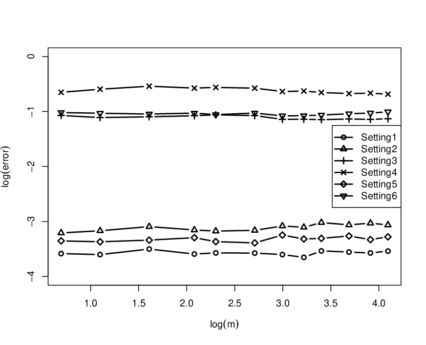
We further investigate the performance of our method with the number of clients increasing. We keep , and split the data onto clients using the same heterogeneous setup. Figure 7 plots the subspace distance against . Each point on the plot is averaged on 200 replications. When the subsample size is small, or the number of clients is large, there is a slightly growing error of FedSSIR. This aligns with Condition (C4) and Lemma 3 that it requires to be not too small to achieve optimal statistical performance. We can see that FedSSIR can efficiently estimate the central subspace as long as is in a reasonable range. Our method has stable performance under different settings.
In order to analysis the impact of different on the simulation results, we conduct a sensitivity experiment against the mixture weight. We keep , and split the data onto clients using the heterogeneous set up. We generate a random vector and with . The smaller the , the more extreme the . The number of dimension reduction directions is chosen by the BIC-type criterion. The penalization parameter is selected by the hold-out validation outlined in section 2.4. The results in Table 2 show that our method performs robustly against the choices of the mixture weight . Our proposal has good performance for datasets with unbalanced sample size.
| \toprule | Setting 1 | Setting 2 | Setting 3 | Setting 4 | Setting 5 | Setting 6 | |
|---|---|---|---|---|---|---|---|
| \midrule | TPR | 1.000 | 1.000 | 0.990 | 1.000 | 1.000 | 0.994 |
| (0) | (0) | (0.056) | (0) | (0) | (0.044) | ||
| FPR | 0.000 | 0.001 | 0.011 | 0.014 | 0.000 | 0.012 | |
| (0.001) | (0.003) | (0.004) | (0.006) | (0.002) | (0.005) | ||
| Dist | 0.033 | 0.044 | 0.419 | 0.388 | 0.033 | 0.417 | |
| (0.016) | (0.022) | (0.132) | (0.114) | (0.018) | (0.097) | ||
| TPR | 1.000 | 1.000 | 0.996 | 1.000 | 1.000 | 1.000 | |
| (0) | (0) | (0.040) | (0) | (0) | (0) | ||
| FPR | 0.000 | 0.001 | 0.011 | 0.013 | 0.000 | 0.012 | |
| (0.001) | (0.002) | (0.004) | (0.005) | (0.001) | (0.003) | ||
| Dist | 0.031 | 0.041 | 0.388 | 0.399 | 0.034 | 0.386 | |
| (0.016) | (0.020) | (0.093) | (0.086) | (0.018) | (0.062) | ||
| TPR | 1.000 | 1.000 | 1.000 | 1.000 | 1.000 | 1.000 | |
| (0) | (0) | (0) | (0) | (0) | (0) | ||
| FPR | 0.000 | 0.000 | 0.011 | 0.013 | 0.000 | 0.011 | |
| (0) | (0.002) | (0.002) | (0.005) | (0) | (0.003) | ||
| Dist | 0.028 | 0.040 | 0.376 | 0.385 | 0.032 | 0.370 | |
| (0.015) | (0.020) | (0.072) | (0.075) | (0.017) | (0.042) |
In addition to the simulations above, we have carried out simulations measuring the performance of our method on non-Gaussian random variables. The results of this experiment are presented in Appendix 8, along with the results of the previous experiments on BIC dimension determination.
4.2 Real Data Analysis
Default of credit card clients dataset (YEH2009dccc) contains 30,000 samples of people with different credit risks. For each subject, there are 23 attributes. First, we separate this dataset into different clients using a heterogeneous pattern, where sample sizes and class proportions on different clients are unbalanced. For class , we generate a random vector with respect to a Dirichlet distribution , where is the concentration parameter that controls the heterogeneity of federated data. Smaller yields more heterogeneous data. Then we generate a random vector from the multinomial distribution . We allocate samples of class to client . Then we partition the samples on each client into a training set and a test set randomly of the same size.
We use logistic regression to construct the classifier and take the average prediction accuracy in the test sets as the testing metric. We compare the performance of the following competitors.
- (M1)
Logistic regression on the aggregated training set. This serves as a benchmark for comparison.
- (M2)
Logistic regression on each client.
- (M3)
Federated sparse sliced inverse regression followed by logistic regression on dimension reduction variables on each client.
- (M4)
Federated principal component analysis by Grammenos et al. grammenos2020fpca followed by logistic regression on dimension reduction variables on each client.
- (M5)
Federated principal component analysis by Chai et al. chai2021fedsvd followed by logistic regression on dimension reduction variables on each client.
We choose the number of the dimension reduction directions for all dimension reduction methods, and the penalization parameter of our method is chosen by cross validation. We repeat this process 100 times to obtain the mean performances of each method and standard deviations. The results are shown in Table 3. It is clearly seen that FedSSIR (M3) performs better than its competitors (M4) and (M5). Also, FedSSIR performs better than local learner (M2) as the number of clients rises, which shows the significance of collaboration. In addition, FedSSIR is comparable to the global model (M1). This indicates that our method successfully captures the low dimensional structure.
| \toprulem | (M1) | (M2) | (M3) | (M4) | (M5) | |
|---|---|---|---|---|---|---|
| \midrule5 | 1 | 79.42(0.77) | 79.18(1.78) | 79.47(1.64) | 74.77(2.91) | 74.77(2.91) |
| 5 | 2 | 79.71(0.70) | 79.86(1.45) | 79.96(1.47) | 75.22(2.51) | 75.22(2.51) |
| 5 | 5 | 80.23(0.52) | 80.68(0.86) | 80.82(0.81) | 76.50(1.48) | 76.50(1.48) |
| 10 | 1 | 79.37(0.60) | 78.66(1.46) | 79.17(1.45) | 74.51(2.34) | 74.51(2.34) |
| 10 | 2 | 79.66(0.57) | 79.13(1.11) | 79.63(1.15) | 74.55(1.74) | 74.55(1.74) |
| 10 | 5 | 80.20(0.37) | 80.24(0.63) | 80.63(0.63) | 76.32(1.06) | 76.33(1.06) |
| 20 | 1 | 79.19(0.45) | 77.55(1.20) | 78.83(1.10) | 73.86(1.75) | 73.87(1.76) |
| 20 | 2 | 79.56(0.42) | 78.46(1.01) | 79.54(0.83) | 74.71(1.54) | 74.71(1.54) |
| 20 | 5 | 80.23(0.38) | 79.64(0.61) | 80.52(0.57) | 76.11(0.92) | 76.11(0.92) |
| 30 | 1 | 79.13(0.37) | 77.06(1.11) | 78.99(0.98) | 73.93(1.60) | 73.94(1.59) |
| 30 | 2 | 79.56(0.35) | 77.74(0.84) | 79.50(0.77) | 74.65(1.18) | 74.65(1.18) |
| 30 | 5 | 80.19(0.33) | 78.92(0.55) | 80.50(0.42) | 75.98(0.68) | 75.98(0.68) |
The other one is the Communities and Crime dataset (misc_communities_and_crime_183). It contains 1,944 observations of communities and 100 predictive features. The task is to predict the total number of violent crimes per 100K population of each sample. We first separate the communities into different clients by their states and select clients with sample size larger than 80 for our experiment. Thus we have 7 clients and a total of 1066 samples. Then we partition the samples on each client into a training set and a test set randomly of the same size.
We use linear regression to construct the model and take the relative prediction error to evaluate the prediction performance, i.e. . We compare the performance of the following competitors.
- (M1)
Linear regression on the aggregated training set. This serves as a benchmark for comparison.
- (M2)
Linear regression on each client.
- (M3)
Federated sparse sliced inverse regression followed by linear regression on dimension reduction variables on each client.
- (M4)
Federated principal component analysis by Grammenos et al. grammenos2020fpca followed by linear regression on dimension reduction variables on each client.
- (M5)
Federated principal component analysis by Chai et al. chai2021fedsvd followed by linear regression on dimension reduction variables on each client.
We choose the number of the dimension reduction directions by BIC-type criterion, and the penalization parameter of our method is chosen by validation. We repeat this process 100 times to obtain mean performances of each method and standard deviations. The results are shown in Table 4. FedSSIR (M3) is significantly superior to the unsupervised learners (M4)-(M5) in regression problems. Local learner (M2) performs badly in this case, which indicates that training with only a single client suffers from lack of data and results in under-fitting. Our FedSSIR method helps in this case, like other federated learning methods. Moreover, FedSSIR performs better than global learner (M1), which shows that our proposal captures the low dimensional structure and enhances the prediction power in the high dimensional case.
| \toprule(M1) | (M2) | (M3) | (M4) | (M5) |
|---|---|---|---|---|
| \midrule0.355(0.024) | 2.059(0.033) | 0.312(0.023) | 0.400(0.022) | 0.398(0.022) |
5 Discussions & Conclusions
Sufficient dimension reduction in the context of federated learning is an exciting topic that hasn’t gained much attention. We devised the FedSSIR algorithm to estimate the sufficient dimension reduction directions in the federated setting. With a -norm penalty term, our method can simultaneously perform dimension reduction and variable selection in the high-dimensional setting. Our simulations and real data experiments show that FedSSIR can perform quite well on heterogeneous data. Also, this approach can easily be extended to other federated learning problems involving generalized eigenvalue decomposition. Nowadays, sufficient dimension reduction on a stochastic data stream is an essential topic in the big data era, see cai2020online; cheng2021online, and how to establish a valid federated sufficient dimension reduction approach on several data streams is also an interesting problem.
6 Derivation of Algorithm 2
In this section, we derive the ADMM algorithm for solving (11).
First, we form the augmented Lagrangian for (14)
| (15) |
where is the dual variable, is the augmented Lagrangian parameter.
The resulting ADMM algorithm is
With a scaled augmented Lagrangian parameter , we can get the scaled form of this algorithm
| (16) | ||||
| (17) | ||||
| (18) |
The scaled version is simpler and easier to work with than the unscaled form.
Update for : (16) is composed of client-specific problems
| (19) |
To solve (16), we adopt the idea of Federated Primal-Dual method (zhang2020fedpd). We will solve the local problem first and average the solutions to get the closed-form update for . We use vectorization operation to convert (19) into a vector minimization form. Let , , , , and . Use the identity , (19) turned into
| (20) |
(20) doesn’t have a closed-form solution, but we can consider a linearized version of it by adding a quadratic term of as suggested by Fang et al. Fang2015GADMM
| (21) |
where . We choose to ensure the convergence of the algorithm.
Convert (21) into matrix optimization version:
| (22) |
where . (22) has the closed-form solution
| (23) |
Therefore, we can get the update of :
Remark 4.
We can write (19) in vectorized form and then the problem is reduced to solving a Lasso regression problem
where . Although plenty of algorithms are proposed to solve Lasso regression problems, this transformation involves a -dimensional Lasso problem in each iteration and increases the computation cost.
Remark 5.
Observe that
Theorem 6 in Fang2015GADMM implies that for some constants ’s. Thus, we have for some constant . According to Lemma 4 in Fang2015GADMM, if , is a solution to (11). A convergence rate for our algorithm is thus established.
Update for : The update of follows directly from Proposition 2 in Kean2018convex.
Proposition 6.
Kean2018convex Let be the singular value decomposition of . Then the optimization problem
has solution satisfies
7 Proof of Theorem 5
It is necessary to show that Lemma 2 and Lemma 3 hold to prove this theorem. In this section, we first show the proofs of Lemma 2 and Lemma 3. Then we are going to prove Theorem 5.
7.1 Proof of Lemma 2
Proof.
For simplify, we assume and since each client’s sample mean and sample size don’t influence the theoretical results in this part. For pair , we have where is the th element of matrix , and is the th element of . Then Lemma 1 in ravikumar2011high implies the results of Lemma 2 here. ∎
7.2 Proof of Lemma 3
Proof.
Recall that are the concomitants of the order statistics and is the inverse regression curve at client . Define the model error of the inverse regression by . Clearly, are also the concomitants of . (2.1) and (2.4) in Yang1977concomitant show that the concomitants are conditionally independent given order statistics and . Then, are zero-mean random vectors and conditionally independent given .
First, we will introduce sub-Gaussian and sub-exponential distributions. For a random variable , define its -norm and -norm as and . Sub-Gaussian random variable is defined to have a -norm less than a constant and sub-exponential random variable is defined to have a -norm less than a constant. The following proposition states the connection between sub-Gaussian and sub-exponential random variables. The proof of it is a direct consequence of Hölder’s inequality and the definitions of sub-Gaussian and sub-exponential random variables.
Proposition 7.
Suppose and are sub-Gaussian random variables, then is sub-exponential and .
Denote the -th element of by , the same for and . Clearly, under Condition (C2), is a sub-Gaussian random variable and its -norm . Proposition 3 in Kean2018convex states that and are also sub-Gaussian random variables with norm and , respectively.
Now, we have
It is easy to see that
| (24) |
where . Then we only need to derive the convergence rate of the foregoing five terms on the right side of (24).
For the th element of , we have
By Condition (C4), there exists some constant , we have , which implies the last inequality above. Thus, we have .
Similarly, for the th element of , we have
Then, following directly from the equivalence of sub-Gaussian properties in Lemma 5.5 in vershynin2011introduction, for some constant , we have
with . Thus, with probability being at least , we have . Taking the union bound, we have
can also be upper bounded similarly.
For the th element of , we have
It requires to show that , and is upper bounded by .
Since , combined with Proposition 7 and the centering lemma in vershynin2018HDP, is sub-exponential with -norm bounded by , where is a constant. Thus, following directly from the Bernstein-type inequality in Proposition 5.16 in vershynin2011introduction, for some sufficiently large constant , we obtain
Also, by taking the union bound, we have
with probability greater than .
Recall that and are conditionally independent sub-Gaussian random vectors with mean zero given the order statistics . Thus, is sub-exponential with mean zero and have a -norm less than , conditionally given the order statistics. Similar to above, by the Berstein-type inequality and taking the union bound, we have
Taking expectation on the order statistics, we have
can also be upper bounded in the same manner. Thus, with probability being at least , is upper bounded by .
For the th element of , we have
This inequality follows from Condition (C3) and (C6). By Lemma C.2 in Agrawal2017rl, we have an inequality against multinomial random vector
Taking the union bound, for some constants , we have
Together with the upper bounds of , , and , we have
with probability being at least for some constant . ∎
7.3 Proof of Theorem 5
Proof.
Before establishing the upper bound on the distance between true and estimated subspaces, we first consider the statistical error of the estimated projection matrix .
Proposition 4 in Kean2018convex states that is the solution of (7) if and only if can be written as , where . Let , , and . can be viewed as the bridge between and . Thus, we obtain
For the term , Lemma 2 in Kean2018convex establishes concentration that given constants and ,
| (25) |
with probability being at least . The second inequality holds by Condition (C5) and the assumption that for some constant .
Let . Following Gao et al. Gao2017scca, we first derive the upper bound and lower bound for . Then we can upper bound with those results.
Upper bound for : First, we want to show that is a feasible solution of (11). We have
and
Since is the optimal solution of (11), we have
Rearrange the variables and use the Hölder’s inequality we have
When , we have
| (26) |
Let , we have . Let be the complementary set of . By the definition of and , we have . Reconsider the LHS of (26),
Thus, we have
| (27) |
Directly from Lemma 3 in Kean2018convex, we obtain
| (28) | ||||
Let . Combining (27) and (28), we have
| (29) | ||||
which implies
| (30) |
Lower bound for : By (29), we have
| (31) |
Using the fact that , we have
| (32) |
Combining (30), (31) and (32), we obtain
| (33) |
(33) shows that lies in a restricted set. We further partition the set into subsets. contains the indices corresponding to the largest entries of , contains the indices corresponding to the second largest entries of , and so forth, with . By the triangle inequality, we have
| (34) | ||||
The definitions of and are deferred to Appendix 9. The second inequality follows directly from the definitions. For , we have
which is combined with (33), to obtain
| (35) | ||||
where the second inequality follows from the Cauchy-Schwarz inequality.
By Condition (C6) and Lemma 6 in Kean2018convex, let , for constant , we have
| (37) |
with probability being at least .
Substituting (37) into (36) and using the assumption that , we have that is lower bounded by some constant when is sufficiently large. Also, is bounded by some constant similarly. Thus we have
| (38) |
Now, we have obtained the upper and lower bound of . Combining (30) and (38) and using the fact that , we have
Squaring both sides, we get
Thus, we have
| (39) |
Recall that . By Lemma 2 and Lemma 2 in Kean2018convex, we have with probability being greater than . Thus . Under Condition (C5) and the assumption that for some constant , we have . Substituting this into (40), we have
| (41) |
Thus, we obtain the upper bound for . Combined with (25), for some constant , we have
| (42) |
with probability being at least .
From Corollary 3.2 in vu2013fantope, for the population central subspace and the estimated subspace , we have
| (43) |
with probability being at least . Combining Corollary 4 with Lemma 7 in Kean2018convex, we can choose , then holds with probability at least , which completes the proof. ∎
8 Dimension determination and other simulation results
8.1 Proof of Corollary 1
We first give the proof of Corollary 1.
Proof.
Theorem 6 in zhu2010cumulative states that converges to in probability, , there exists that for ,
Suppose there are clients making correct decision of but , then there must exist a that at least clients choosing . This means if , there are at least clients making the wrong decision. Thus, let be a permutation of , we have
∎
8.2 Simulation on non-Gaussian covariates
We conduct a simulation to show the performance of our proposal on non-Gaussian covariates. We generate non-Gaussian covariates in the following way. Let , where is generated same as before and the elements of are sampled independently from Bernoulli distribution. Since and are independently sampled from sub-Gaussian distributions, is also a sub-Gaussian random vector, but not Gaussian.
| \toprule | Setting 1 | Setting 2 | Setting 3 | Setting 4 | Setting 5 | Setting 6 | |
|---|---|---|---|---|---|---|---|
| \midruleFedSSIR | TPR | 1.000 | 1.000 | 0.963 | 0.851 | 1.000 | 0.950 |
| (0) | (0) | (0.117) | (0.210) | (0) | (0.133) | ||
| FPR | 0.000 | 0.002 | 0.005 | 0.007 | 0.000 | 0.011 | |
| (0.001) | (0.005) | (0.011) | (0.012) | (0.002) | (0.013) | ||
| Dist | 0.050 | 0.075 | 0.462 | 0.683 | 0.059 | 0.459 | |
| (0.030) | (0.035) | (0.277) | (0.348) | (0.029) | (0.246) | ||
| SSIR | TPR | 1.000 | 1.000 | 0.764 | 0.571 | 1.000 | 0.989 |
| (0) | (0) | (0.250) | (0.386) | (0) | (0.064) | ||
| FPR | 0.928 | 0.918 | 0.517 | 0.280 | 0.199 | 0.032 | |
| (0.092) | (0.105) | (0.269) | (0.265) | (0.330) | (0.147) | ||
| Dist | 1.819 | 1.544 | 1.802 | 1.620 | 0.877 | 0.488 | |
| (0.134) | (0.251) | (0.166) | (0.152) | (0.538) | (0.333) | ||
| LassoSIR | TPR | 1.000 | 1.000 | 0.969 | 0.997 | 1.000 | 0.999 |
| (0) | (0) | (0.090) | (0.032) | (0) | (0.014) | ||
| FPR | 0.327 | 0.270 | 0.682 | 0.991 | 0.395 | 0.996 | |
| (0.114) | (0.104) | (0.350) | (0.074) | (0.406) | (0.057) | ||
| Dist | 0.136 | 0.141 | 1.777 | 1.776 | 1.176 | 1.328 | |
| (0.092) | (0.063) | (0.590) | (0.523) | (0.718) | (0.367) |
We keep , and split the data onto clients using the following heterogeneous set up. We generate a random vector and with . The number of dimension reduction directions is chosen by the BIC-type criterion. The penalization parameter is selected by the hold-out validation outlined in section 2.4. We also include the results of SSIR and LassoSIR. The results are shown in Table 5. We can see that our method still performs well on non-Gaussian covariates.
8.3 Dimension determination results
Here, we also report the proportion of correct decisions about the dimension of the central subspace in our simulations in Table 6. We can see that BIC type criterion has a satisfactory performance in most cases. As the sample size grows, the performance becomes better, which is consistent with our conclusion that converges to in probability. Our proposed BIC has similar performance under different settings, which reflects that our method performs well for unbalanced datasets. Compared with the other two methods, our proposed BIC performs more robustly under the non-Gaussian setting.
| \toprule | Setting 1 | Setting 2 | Setting 3 | Setting 4 | Setting 5 | Setting 6 | |
|---|---|---|---|---|---|---|---|
| \midrulen = 100 | BIC | 1.000 | 0.950 | 0.785 | 0.855 | 1.000 | 0.805 |
| SSIR | 0.020 | 0.350 | 0.575 | 0.065 | 0.430 | 0.530 | |
| LassoSIR | 1.000 | 1.000 | 0.030 | 0.055 | 1.000 | 0.525 | |
| n = 200 | BIC | 1.000 | 0.995 | 0.825 | 0.865 | 1.000 | 0.875 |
| SSIR | 0.015 | 0.290 | 0.450 | 0.065 | 0.410 | 0.615 | |
| LassoSIR | 0.995 | 1.000 | 0.035 | 0.100 | 1.000 | 0.995 | |
| \midrule | BIC | 1.000 | 1.000 | 0.960 | 0.985 | 1.000 | 0.980 |
| BIC | 1.000 | 1.000 | 0.985 | 0.995 | 1.000 | 0.995 | |
| BIC | 1.000 | 1.000 | 0.995 | 1.000 | 1.000 | 1.000 | |
| \midrulenon-Gaussian | BIC | 1.000 | 1.000 | 0.840 | 0.760 | 1.000 | 0.870 |
| SSIR | 0.015 | 0.385 | 0.645 | 0.045 | 0.365 | 0.790 | |
| LassoSIR | 0.995 | 1.000 | 0.025 | 0.010 | 0.700 | 0.010 |
9 Auxiliary definitions
Here are some definitions used in the text. Let be the order statistics of . Define the inverse regression function and let . Total variation for a vector-valued function under the norm is defined as below.
Definition 1.
Let be the collection of all -point partitions on the interval , where and . A vector-valued function is said to have a total variation defined as .
Meinshausen and Yu Meinshausen2009lassohigh gave a definition on the -sparse eigenvalue of a matrix .
Definition 2.
The -sparse minimal and maximal eigenvalues of are
There are two consistent estimators for . Hsing and Carroll hsing1992asym gave a two slice estimation . Let be the order statistics of responses. is denoted as the value of associated with and termed the concomitant of . Then the estimator is
| (44) |
where is the floor function that returns the greatest integer less than or equal to the input.
Zhu and Ng zhu1995asymptotics gave another estimator for . First, partition the dataset into slices with respect to the order statistics of and let be the indice sets for each slice. Then, the estimator is obtained by computing the average of covariance matrices on each slice:
| (45) |
Therefore, a trivial estimator for is .
Similar to 2.1, we derive the population and empirical average conditional covariance matrices. Let , the population average conditional covariance matrix can be represented as . Thus, the empirical average conditional covariance matrix .
References
- (1) Kairouz, P., McMahan, H.B., Avent, B., Bellet, A., Bennis, M., Bhagoji, A.N., Bonawitz, K., Charles, Z., Cormode, G., Cummings, R., et al.: Advances and open problems in federated learning. Foundations and Trends® in Machine Learning 14(1–2), 1–210 (2021). https://doi.org/10.1561/2200000083
- (2) Yang, Q., Liu, Y., Cheng, Y., Kang, Y., Chen, T., Yu, H.: Federated learning. Synthesis LectureYs on Artificial Intelligence and Machine Learning 13(3), 1–207 (2019)
- (3) McMahan, B., Moore, E., Ramage, D., Hampson, S., y Arcas, B.A.: Communication-efficient learning of deep networks from decentralized data. In: Artificial Intelligence and Statistics, pp. 1273–1282 (2017). PMLR
- (4) Li, T., Sahu, A.K., Zaheer, M., Sanjabi, M., Talwalkar, A., Smith, V.: Federated optimization in heterogeneous networks. Proceedings of Machine Learning and Systems 2, 429–450 (2020)
- (5) Karimireddy, S.P., Kale, S., Mohri, M., Reddi, S., Stich, S., Suresh, A.T.: Scaffold: Stochastic controlled averaging for federated learning. In: International Conference on Machine Learning, pp. 5132–5143 (2020). PMLR
- (6) Yuan, H., Ma, T.: Federated accelerated stochastic gradient descent. Advances in Neural Information Processing Systems 33, 5332–5344 (2020)
- (7) Grammenos, A., Mendoza Smith, R., Crowcroft, J., Mascolo, C.: Federated principal component analysis. Advances in Neural Information Processing Systems 33, 6453–6464 (2020)
- (8) Chai, D., Wang, L., Fu, L., Zhang, J., Chen, K., Yang, Q.: Federated singular vector decomposition. arXiv preprint arXiv:2105.08925 (2021)
- (9) Li, K.-C.: Sliced inverse regression for dimension reduction. Journal of the American Statistical Association 86(414), 316–327 (1991). https://doi.org/10.2307/2290568
- (10) Cook, R.D.: On the interpretation of regression plots. Journal of the American Statistical Association 89(425), 177–189 (1994). https://doi.org/10.1080/01621459.1994.10476459
- (11) Zeng, P., Zhu, Y.: An integral transform method for estimating the central mean and central subspaces. Journal of Multivariate Analysis 101(1), 271–290 (2010). https://doi.org/10.1016/j.jmva.2009.08.004
- (12) Cook, R.D.: Save: a method for dimension reduction and graphics in regression. Communications in Statistics - Theory and Methods 29(9-10), 2109–2121 (2000). https://doi.org/10.1080/03610920008832598
- (13) Cook, R.D., Ni, L.: Sufficient dimension reduction via inverse regression. Journal of the American Statistical Association 100(470), 410–428 (2005). https://doi.org/10.1198/016214504000001501
- (14) Li, B., Wang, S.: On directional regression for dimension reduction. Journal of the American Statistical Association 102(479), 997–1008 (2007). https://doi.org/10.1198/016214507000000536
- (15) Li, K.-C.: On principal hessian directions for data visualization and dimension reduction: Another application of stein’s lemma. Journal of the American Statistical Association 87(420), 1025–1039 (1992). https://doi.org/10.1080/01621459.1992.10476258
- (16) Xia, Y., Tong, H., Li, W.K., Zhu, L.-X.: An adaptive estimation of dimension reduction space. Journal of The Royal Statistical Society Series B-statistical Methodology 64(3), 363–410 (2002). https://doi.org/10.1142/9789812836281_0023
- (17) Hsing, T., Carroll, R.J.: An asymptotic theory for sliced inverse regression. The Annals of Statistics 20(2), 1040–1061 (1992). https://doi.org/10.1214/aos/1176348669
- (18) Zhu, L.-X., Ng, K.W.: Asymptotics of sliced inverse regression. Statistica Sinica 102, 727–736 (1995). https://doi.org/10.1007/BF01192467
- (19) Zhu, L.-X., Miao, B.-Q., Peng, H.: On sliced inverse regression with high-dimensional covariates. Journal of the American Statistical Association 101(474), 630–643 (2006). https://doi.org/10.2307/27590723
- (20) Li, L., Dennis Cook, R., Nachtsheim, C.J.: Model-free variable selection. Journal of the Royal Statistical Society: Series B (Statistical Methodology) 67(2), 285–299 (2005). https://doi.org/10.1111/j.1467-9868.2005.00502.x
- (21) Li, L., Yin, X.: Sliced inverse regression with regularizations. Biometrics 64(1), 124–131 (2008). https://doi.org/10.1111/j.1541-0420.2007.00836.x
- (22) Lin, Q., Zhao, Z., Liu, J.S.: Sparse sliced inverse regression via lasso. Journal of the American Statistical Association 114(528), 1726–1739 (2019). https://doi.org/10.1080/01621459.2018.1520115. PMID: 32952234
- (23) Chen, X., Zou, C., Cook, R.D.: Coordinate-independent sparse sufficient dimension reduction and variable selection. The Annals of Statistics 38(6), 3696–3723 (2010). https://doi.org/10.1214/10-AOS826
- (24) Tan, K.M., Wang, Z., Zhang, T., Liu, H., Cook, R.: A convex formulation for high-dimensional sparse sliced inverse regression. Biometrika 105, 769–782 (2018). https://doi.org/10.1093/biomet/asy049
- (25) Boyd, S., Parikh, N., Chu, E., Peleato, B., Eckstein, J., et al.: Distributed optimization and statistical learning via the alternating direction method of multipliers. Foundations and Trends® in Machine learning 3(1), 1–122 (2011). https://doi.org/10.1561/2200000016
- (26) Fang, E., He, B.-S., Liu, H., Yuan, X.: Generalized alternating direction method of multipliers: New theoretical insights and applications. Mathematical Programming Computation 7, 149–187 (2015). https://doi.org/10.1007/s12532-015-0078-2
- (27) Zhang, X., Hong, M., Dhople, S., Yin, W., Liu, Y.: Fedpd: A federated learning framework withadaptivity to non-iid data. IEEE Transactions on Signal Processing 69, 6055–6070 (2021). https://doi.org/10.1109/TSP.2021.3115952
- (28) Hsieh, K., Phanishayee, A., Mutlu, O., Gibbons, P.: The non-iid data quagmire of decentralized machine learning. In: International Conference on Machine Learning, pp. 4387–4398 (2020). PMLR
- (29) Eaton, M.L.: A characterization of spherical distributions. Journal of Multivariate Analysis 20(2), 272–276 (1986). https://doi.org/10.1016/0047-259X(86)90083-7
- (30) Hall, P., Li, K.-C.: On almost linearity of low dimensional projections from high dimensional data. The Annals of Statistics 21(2), 867–889 (1993). https://doi.org/10.1214/aos/1176349155
- (31) Shimodaira, H.: Improving predictive inference under covariate shift by weighting the log-likelihood function. Journal of Statistical Planning and Inference 90, 227–244 (2000). https://doi.org/10.1016/S0378-3758(00)00115-4
- (32) Vu, V.Q., Cho, J., Lei, J., Rohe, K.: Fantope projection and selection: A near-optimal convex relaxation of sparse pca. In: Advances in Neural Information Processing Systems 26, vol. 26, pp. 2670–2678 (2013)
- (33) Absil, P.-A., Mahony, R., Sepulchre, R.: Optimization Algorithms on Matrix Manifolds. Princeton University Press, Princeton (2009). https://doi.org/10.1515/9781400830244
- (34) Li, B.: Sufficient Dimension Reduction : Methods and Applications with R. Chapman and Hall/CRC Press, Boca Raton (2017). https://doi.org/10.1201/9781315119427
- (35) Zhu, L.-P., Zhu, L.-X., Feng, Z.-H.: Dimension reduction in regressions through cumulative slicing estimation. Journal of the American Statistical Association 105(492), 1455–1466 (2010). https://doi.org/10.1198/jasa.2010.tm09666
- (36) Vershynin, R.: Introduction to the non-asymptotic analysis of random matrices. arXiv preprint arXiv:1011.3027 (2010). https://doi.org/10.1017/CBO9780511794308.006
- (37) Vershynin, R.: High-Dimensional Probability: An Introduction with Applications in Data Science. Cambridge Series in Statistical and Probabilistic Mathematics. Cambridge University Press, Cambridge (2018). https://doi.org/10.1017/9781108231596
- (38) Meinshausen, N., Yu, B.: Lasso-type recovery of sparse representations for high-dimensional data. The Annals of Statistics 37(1), 246–270 (2009). https://doi.org/10.1214/07-AOS582
- (39) Zhang, C.-H.: Nearly unbiased variable selection under minimax concave penalty. The Annals of statistics 38(2), 894–942 (2010). https://doi.org/10.1214/09-AOS729
- (40) Ravikumar, P., Wainwright, M.J., Raskutti, G., Yu, B.: High-dimensional covariance estimation by minimizing l1-penalized log-determinant divergence. Electronic Journal of Statistics 5, 935–980 (2011). https://doi.org/10.1214/11-EJS631
- (41) Caldas, S., Duddu, S.M.K., Wu, P., Li, T., Konečný, J., McMahan, H.B., Smith, V., Talwalkar, A.: Leaf: A benchmark for federated settings. arXiv preprint arXiv:1812.01097 (2019)
- (42) Yeh, I.-C., Lien, C.-h.: The comparisons of data mining techniques for the predictive accuracy of probability of default of credit card clients. Expert Systems with Applications 36(2, Part 1), 2473–2480 (2009). https://doi.org/10.1016/j.eswa.2007.12.020
- (43) Redmond, M.: Communities and Crime. UCI Machine Learning Repository (2009)
- (44) Cai, Z., Li, R., Zhu, L.: Online sufficient dimension reduction through sliced inverse regression. Journal of Machine Learning Research 21(10), 1–25 (2020)
- (45) Cheng, H., Cui, W., Jianjun, X.: Online sparse sliced inverse regression. arXiv preprint arXiv:2009.14615 (2021)
- (46) Yang, S.S.: General distribution theory of the concomitants of order statistics. The Annals of Statistics 5(5), 996–1002 (1977). https://doi.org/10.1214/aos/1176343954
- (47) Agrawal, S., Jia, R.: Optimistic posterior sampling for reinforcement learning: worst-case regret bounds. In: Advances in Neural Information Processing Systems, vol. 30, pp. 1184–1194 (2017). Curran Associates, Inc.
- (48) Gao, C., Ma, Z., Zhou, H.: Sparse cca: Adaptive estimation and computational barriers. The Annals of Statistics 45, 2074–2101 (2017). https://doi.org/10.1214/16-AOS1519