Hot Big Bang from inflation without the inflaton reheating
Abstract
According to the standard lore, a prolonged inflation leaves a quantum field theory in a cold, low entropy state. Thus, some mechanism is needed to reheat this post-inflationary state, leaving a hot, thermal, radiation-dominated Universe. Typically, reheating is achieved coupling the inflaton field to the QFT degrees of freedom. We argue that the nonequilibrium dynamics of a non-conformal QFT in (post-)inflationary background space-time can produce hot quark-gluon plasma with the reheating temperature of order the inflationary Hubble scale, without the inflaton coupling.
Introduction and summary.– A common assumption is that the elementary particles populating the Universe were created during the process of reheating the Standard Model after inflation Linde 1987. The basic idea Kofman et al. 1997 is that the elementary particles are produced from interactions with the oscillating inflaton. The process of reheating completes when almost all the energy of the inflaton is transferred to the thermal energy of the Standard Model particles, and the inflaton settles in the minimum of its effective potential. We have yet to observe the inflaton field, therefore it is sensible to ask the question whether a post-inflationary quantum field theory state can be intrinsically reheated during the inflationary exit stage. In other words, can we decouple the dynamics of the pre-Big Bang cosmological background space-time from the reheating, thus alleviating the pressure on Particle Physics to detect the inflaton in the collider experiments?
In this Letter we present precisely such scenario. The main point is that a nonconformal QFT state, right before the exit from the accelerated background state-time expansion, taken for simplicity here to be a de Sitter space-time, is not a Bunch-Davies vacuum, but rather is a dynamical fixed point (DFP) Buchel and Karapetyan 2017; Buchel 2022a: it is characterized by a constant entropy production rate. Specifically, if is a scale factor of the QFT background -dimensional Friedmann-Lemaitre-Robertson-Walker (FLRW) Universe
| (1) |
the entropy production rate is given by
| (2) | |||||
where the comoving and the physical entropy densities are related as
| (3) |
Specializing to de Sitter Universe, i.e., , in variety of strongly coupled nonconformal QFTs with a holographic dual, the entropy production rate was shown to be nonzero Buchel and Karapetyan 2017; Buchel 2018; Buchel 2020,
| (4) |
where the constant de Sitter physical entropy density is called the vacuum entanglement entropy (VEE) density Buchel 2017a.
Consider now a simple model of exit from the accelerated expansion, where the Hubble parameter evolves as
| (5) |
Here the constant energy scale specifies the exit-rate from the inflation, and the scale parameter is normalized as . For a rough estimate, in this model the exit from inflation occurs during the time frame , so that the scale factor changes as
| (6) |
During the inflationary exit, the comoving entropy density can only increase (2), so
| (7) |
where we denoted by the physical entropy density of the post-inflationary QFT state. From (7) we conclude that
| (8) |
The post-inflationary state e is nonequilibrium; its subsequent evolution leads to its thermalization with the thermal entropy density . Since the equilibration of the post-inflationary state occurs in a microcanonical ensemble, i.e., at constant energy density, from its energy density at the inflationary exist, and the equilibrium equation of state of the QFT plasma, we can predict its thermalization - the reheating - temperature. In what follows we implement the outlined argument in a precise holographic model. The use of the holographic correspondence Maldacena 1999 is a required computational tool if we want to reliably discuss the nonequilibrium dynamics of strongly coupled gauge theories.
The model.– We consider a simple11 1 Reheating in more realistic models of Buchel 2019; Buchel 2020; Buchel 2022c will be discussed elsewhere. holographic toy model of a -dimensional massive with the effective dual gravitational action22 2 We set the radius of an asymptotic geometry to unity.:
| (9) |
The four dimensional gravitational constant is related to the ultraviolet (UV) conformal fixed point central charge as
| (10) |
is a gravitational bulk scalar with
| (11) |
which is dual to a dimension operator of the boundary theory. is a relevant deformation of the UV with
| (12) |
with being the deformation mass scale. Thermodynamics of the boundary plasma was discussed in Buchel and Pagnutti 2010, the thermalization of the theory in was studied in Bosch et al. 2017, and the de Sitter DFPs of the theory were analyzed in Buchel 2018. de Sitter DFPs of the model discussed are stable Buchel 2018; Buchel 2022b.
We study dynamics in FLRW Universe with the Hubble parameter evolving as in (5). A generic state of the boundary field theory with a gravitational dual (9), homogeneous and isotropic in the spatial boundary coordinates , leads to a bulk gravitational metric ansatz
| (13) |
with the warp factors as well as the bulk scalar depending only on . From the effective action (9) we obtain the following equations of motion:
| (14) |
as well as the Hamiltonian constraint equation:
| (15) |
and the momentum constraint equation:
| (16) |
In (14)-(16) we denoted , , and . The near-boundary asymptotic behavior of the metric functions and the scalar encode the mass parameter and the boundary metric scale factor :
| (17) |
in (17) is the residual radial coordinate diffeomorphism parameter Chesler and Yaffe 2014. An initial state of the boundary field theory is specified providing the scalar profile and solving the constraint (15), subject to the boundary conditions (17). Equations (14) can then be used to evolve the state.
The subleading terms in the boundary expansion of the metric functions and the scalar encode the evolution of the energy density , the pressure and the expectation values of the operator of the prescribed boundary QFT initial state. Specifically, extending the asymptotic expansion (17) for ,
| (18) |
the observables of interest can be computed following the holographic renormalization of the model:
| (19) | |||
| (20) | |||
| (21) |
where the terms in brackets, depending on arbitrary constants , encode the renormalization scheme ambiguities. Independent of the renormalization scheme, these expectation values satisfy the expected conformal Ward identity
| (22) |
Furthermore, the conservation of the stress-energy tensor
| (23) |
is a consequence of the momentum constraint (16):
| (24) |
From now on we choose a scheme with .
One of the advantages of the holographic formulation of a QFT dynamics is the natural definition of its far-from-equilibrium entropy density. A gravitational geometry (13) has an apparent horizon located at , where Chesler and Yaffe 2014
| (25) |
Following Booth 2005; Figueras et al. 2009 we associate the non-equilibrium entropy density of the boundary QFT with the Bekenstein-Hawking entropy density of the apparent horizon
| (26) |
Using the holographic background equations of motion (14)-(16) we find
| (27) |
Following Buchel and Karapetyan 2017 it is easy to prove that the entropy production rate as defined by (27) is non-negative, i.e.,
| (28) |
in holographic dynamics governed by (14)-(16). We implement the holographic evolution as explained in Buchel 2022a, adopting numerical codes developed in Bosch et al. 2017; Buchel 2017b; Buchel 2018; Buchel 2022a.
Consider the dynamics of the system in the inflationary-exit time window, defined as . For , the model is in a de Sitter DFP33 3 In practice we initialize the system in an arbitrary spatially homogeneous and isotropic state at and let it evolve to an appropriate de Sitter DFP attractor, uniquely specified by the ratio Buchel 2018., and by the Hubble parameter is vanishingly small, so that the subsequent dynamics is effectively in the Minkowski space-time with the constant scale factor and the constant energy density (see (19) and (24)). Thus, the evolution for is just a thermalization of the post-inflationary state with a fixed energy density , which following Bosch et al. 2017 would thermalize as to an equilibrium state with . The thermal features of the final equilibrium state, including its temperature — the reheating temperature we are after — can be read off from the equation of state of the equilibrium quark-gluon plasma of the model determined in Buchel and Pagnutti 2010.


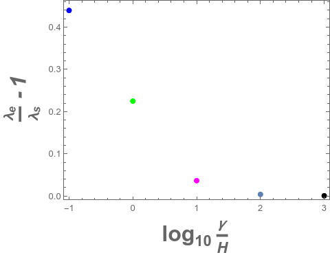
We find44 4 Additional details regarding the simulations can be found in the supplemental material. that the maximal reheating temperature occurs when the exit from the de Sitter (inflationary) phase is very rapid . In this regime effectively all of the energy density of the pre-exit DFP state is converted into the energy density . In the limit there is effectively no expansion of the Universe in the exit time-window (see (6)), so there is no ’dilution’ of the energy density. In this parametric regime, there is a clear separation of two processes: the exit from the accelerated expansion, and the following equilibration of the post-exit state. The time scale of the former is set by , while the time scale of the latter is determined by the thermalization (reheating) temperature Buchel et al. 2015; Buchel and Day 2015; Attems et al. 2016; Janik et al. 2016. For the two processes become intertwined, the scale factor of the Universe can noticeably increase, resulting in the dilution of the energy density leading to , and ultimately decreasing the reheating temperature. Results of the numerical analysis are presented in Figs. 1,2. The red dashed curve in the left panel represents the near-conformal, i.e., , approximation to the maximal reheating temperature55 5 It can be analytically computed using the near-conformal description of the de Sitter DFPs of the model Buchel 2018 and its equilibrium thermodynamics. ,
| (29) |
Notice that the reheating temperature vanishes in the conformal limit — (unjustified) expectations that non-conformal theories have trivial de Sitter vacua, rather than de Sitter DFPs, was the prime reason for the inflaton reheating models Kofman et al. 1997.
Conclusions.– We argued that the reheating of a post-inflationary state of a nonconformal quantum field theory can be achieved entirely due to the nonequilibrium dynamics in the inflationary exit. The reheating temperature is the larger the more rapid the exit from inflation occurs, and the larger the scale invariance of the QFT is broken compare to the inflationary Hubble scale . In the model discussed we observed the reheating temperatures of order for the mass parameter of the theory .
The main open problem is understanding de Sitter DFPs from purely QFT perspective. Whenever the exit from the accelerated expansion is very rapid, the pre-thermalized state of the theory is very close to that of the corresponding DFP; this universality suggests that in this case there might be observable phenomenological imprints of the dynamical fixed point of the theory on the Hot Big Bang cosmology.
The reheating mechanism described in this Letter is that of the gravitational reheating66 6 See Akrami et al. 2018 for a recent review and additional references.. In this sense it is similar to preheating in ”non-oscillatory models” (NO) Peebles and Vilenkin 1999; Felder et al. 1999. The difference is related to the question, what is the energy being released upon the exit from inflation? This is the crucial issue, since once the energy is released, the corresponding QFT state will simply equilibrate to the thermal one at this particular energy density. The energy released at the end of inflation in NO models is the energy of the produced particles during the inflationary exit. On the contrary, here, it is the energy density of the de Sitter state of the strongly coupled non-conformal theory that is being released — very little energy density is being produced during the (rapid) inflationary exit. In fact, the more rapid the exit, the less additional energy is being produced (see the supplemental material).
Acknowledgements.
We would like to thank A. Linde for valuable correspondence regarding preheating in NO models. Research at Perimeter Institute is supported in part by the Government of Canada through the Department of Innovation, Science and Economic Development Canada and by the Province of Ontario through the Ministry of Colleges and Universities. This work is further supported by a Discovery Grant from the Natural Sciences and Engineering Research Council of Canada.Supplemental material.– We use numerical code developed in Buchel 2018; Buchel 2022a to evolve the holographic model (9) in FLRW Universe (5) — the modifications are minimal as the evolution equations (14) are sensitive only to (and not its derivatives), which is set to unity in Buchel 2018; Buchel 2022a for the study of the de Sitter DFPs of the model. This change neither affects the convergence nor the stability of the code for inflationary exit simulations over the wide range of . In what follows we present main simulation results to collaborate the statements in the Letter. We focus on simulations with .

In Figs. 3,4 we present the relative change of the gravitational bulk scalar and the diffeomorphism parameter (see (18)) during the inflationary exit for select values of . Here, the profile of the scalar at the inflationary exit start, , is identical to that of corresponding de Sitter dynamical fixed point; while indicates the scalar profile at the end of the inflationary exit. Similar notations are used for the parameter . We use consistent color coding throughout the supplemental material, so that
| (30) |
The main message is that the more rapid the exit from inflation is, i.e., the larger is the ratio , the more the exit state e resembles that of the pre-exit de Sitter dynamical fixed point77 7 This is a different universality from the abrupt holographic quenches of the relevant couplings of the boundary QFT studied in Buchel et al. 2013..

Thus, it is not a surprise that there is less energy density change in the inflationary exit, the more abrupt this exit is, see Fig. 5. At the start of the exit, i.e., for , the energy density is that of the de Sitter DFP of the holographic model (9) with . Notice that the physical energy density decreases for more gradual exit rates (the blue curve) — this is because for smaller values of the Universe can substantially expand in the exit window .

As an important check on our numerics, we can analytically predict the energy density change in the inflationary exit window in the abrupt exit limit. Indeed, using the fact that in the limit both and are nearly constant,
| (31) |
we can integrate (24):
| (32) |
Thus, as and dropping , we find
| (33) |
Results for for inflationary exits with rates (30), along with the analytic approximation (the solid red curve) (33) are presented in Fig. 6.


In Figs. 7,8 we present the evolution of the physical and the comoving entropy density of our holographic model in the inflationary exits with rates88 8 We do not provide the plot for the comoving entropy density for the evolution with . Given the vast expansion of the Universe in this case, , it would completely overwhelm the other results. given by (30). Note that at the start of the inflationary exits, the physical entropy density is the same for all the exit rates. It is nothing but the vacuum entanglement entropy density (see (4)) of the corresponding de Sitter DFP of the model. On the contrary, the comoving entropy densities are very different: , where the scale factor is
| (34) |
The physical entropy density initially decreases (due to the continual expansion of the Universe in the inflationary exit), but close to the end of the inflationary exit, i.e., for , it starts to increase, representing the thermalization of the inflationary post-exit state of the model in Minkowski space-time. Following (28), the comoving entropy density always increases throughout the full dynamics.
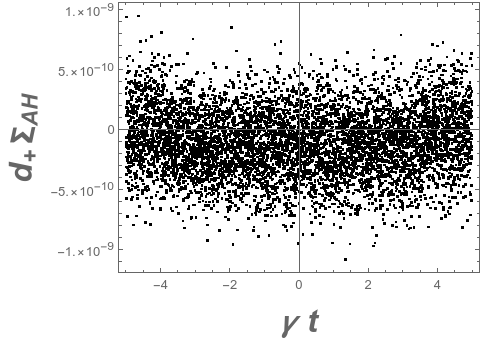
The final comment is related to one of the many checks we performed on our numerical code. During the evolution, the computational domain stays fixed, , with corresponding to the asymptotic boundary, and representing the apparent horizon of the dual gravitational bulk. An important test is monitoring the constraint (25) throughout the full evolution. In Fig. 9 we present , evaluated at the apparent horizon, during the inflationary exit with .
References
- Linde (1987) A. D. Linde, Phys. Today 40, 61 (1987).
- Kofman et al. (1997) L. Kofman, A. D. Linde, and A. A. Starobinsky, Phys. Rev. D 56, 3258 (1997), arXiv:hep-ph/9704452 .
- Buchel and Karapetyan (2017) A. Buchel and A. Karapetyan, JHEP 03, 114 (2017), arXiv:1702.01320 [hep-th] .
- Buchel (2022a) A. Buchel, JHEP 02, 128 (2022a), arXiv:2111.04122 [hep-th] .
- Buchel (2018) A. Buchel, Nucl. Phys. B928, 307 (2018), arXiv:1707.01030 [hep-th] .
- Buchel (2020) A. Buchel, JHEP 05, 035 (2020), arXiv:1912.03566 [hep-th] .
- Buchel (2017a) A. Buchel, (2017a), arXiv:1702.08590 [hep-th] .
- Maldacena (1999) J. M. Maldacena, Int. J. Theor. Phys. 38, 1113 (1999), [Adv. Theor. Math. Phys.2,231(1998)], arXiv:hep-th/9711200 [hep-th] .
- (9) Reheating in more realistic models of Buchel 2019; Buchel 2020; Buchel 2022c will be discussed elsewhere.
- (10) We set the radius of an asymptotic geometry to unity.
- Buchel and Pagnutti (2010) A. Buchel and C. Pagnutti, Nucl. Phys. B 824, 85 (2010), arXiv:0904.1716 [hep-th] .
- Bosch et al. (2017) P. Bosch, A. Buchel, and L. Lehner, JHEP 07, 135 (2017), arXiv:1704.05454 [hep-th] .
- Buchel (2022b) A. Buchel, JHEP 09, 227 (2022b), arXiv:2207.09887 [hep-th] .
- Chesler and Yaffe (2014) P. M. Chesler and L. G. Yaffe, JHEP 07, 086 (2014), arXiv:1309.1439 [hep-th] .
- Booth (2005) I. Booth, Can. J. Phys. 83, 1073 (2005), arXiv:gr-qc/0508107 [gr-qc] .
- Figueras et al. (2009) P. Figueras, V. E. Hubeny, M. Rangamani, and S. F. Ross, JHEP 04, 137 (2009), arXiv:0902.4696 [hep-th] .
- Buchel (2017b) A. Buchel, JHEP 08, 134 (2017b), arXiv:1705.08560 [hep-th] .
- (18) In practice we initialize the system in an arbitrary spatially homogeneous and isotropic state at and let it evolve to an appropriate de Sitter DFP attractor, uniquely specified by the ratio Buchel 2018.
- (19) Additional details regarding the simulations can be found in the supplemental material.
- Buchel et al. (2015) A. Buchel, M. P. Heller, and R. C. Myers, Phys. Rev. Lett. 114, 251601 (2015), arXiv:1503.07114 [hep-th] .
- Buchel and Day (2015) A. Buchel and A. Day, Phys. Rev. D 92, 026009 (2015), arXiv:1505.05012 [hep-th] .
- Attems et al. (2016) M. Attems, J. Casalderrey-Solana, D. Mateos, I. Papadimitriou, D. Santos-Oliván, C. F. Sopuerta, M. Triana, and M. Zilhão, JHEP 10, 155 (2016), arXiv:1603.01254 [hep-th] .
- Janik et al. (2016) R. A. Janik, J. Jankowski, and H. Soltanpanahi, JHEP 06, 047 (2016), arXiv:1603.05950 [hep-th] .
- (24) It can be analytically computed using the near-conformal description of the de Sitter DFPs of the model Buchel 2018 and its equilibrium thermodynamics.
- (25) See Akrami et al. 2018 for a recent review and additional references.
- Peebles and Vilenkin (1999) P. J. E. Peebles and A. Vilenkin, Phys. Rev. D 59, 063505 (1999), arXiv:astro-ph/9810509 .
- Felder et al. (1999) G. N. Felder, L. Kofman, and A. D. Linde, Phys. Rev. D 60, 103505 (1999), arXiv:hep-ph/9903350 .
- (28) This is a different universality from the abrupt holographic quenches of the relevant couplings of the boundary QFT studied in Buchel et al. 2013.
- (29) We do not provide the plot for the comoving entropy density for the evolution with . Given the vast expansion of the Universe in this case, , it would completely overwhelm the other results.
- Buchel (2019) A. Buchel, Nucl. Phys. B 948, 114769 (2019), arXiv:1904.09968 [hep-th] .
- Buchel (2022c) A. Buchel, (2022c), arXiv:2210.17380 [hep-th] .
- Akrami et al. (2018) Y. Akrami, R. Kallosh, A. Linde, and V. Vardanyan, JCAP 06, 041 (2018), arXiv:1712.09693 [hep-th] .
- Buchel et al. (2013) A. Buchel, R. C. Myers, and A. van Niekerk, Phys. Rev. Lett. 111, 201602 (2013), arXiv:1307.4740 [hep-th] .