跳到论文正文
W Papers独立论文阅读器 arXiv:2301.09248 论文正文 计算阅读时间 · 0%
引用这篇论文根据当前论文元数据生成,正式投稿前建议核对。


License: arXiv.org perpetual non-exclusive license
arXiv:2301.09248v1 [eess.SP] 23 Jan 2023

Target-Mounted Intelligent Reflecting Surface for Joint Location and Orientation Estimation Thanks: Peilan Wang and Jun Fang are with the National Key Laboratory of Science and Technology on Communications, University of Electronic Science and Technology of China, Chengdu, China 611731 (e-mail: peilan_wangle@std.uestc.edu.cn, JunFang@uestc.edu.cn).Thanks: Weidong Mei is with the Department of Electrical and Computer Engineering, National University of Singapore, Singapore, 117583 (e-mail: wmei@nus.edu.sg). Thanks: Rui Zhang is with the The Chinese University of Hong Kong, Shenzhen, and Shenzhen Research Institute of Big Data, Shenzhen, China, 518172 (e-mail: rzhang@cuhk.edu.cn). He is also with the Department of Electrical and Computer Engineering, National Uiversity of Singapore, Singapore 117583 (e-mail: elezhang@nus.edu.sg).

Peilan Wang    Weidong Mei    Affiliation: Jun Fang,  , and Rui Zhang,  
Abstract

Intelligent reflecting surface (IRS) has been widely recognized as an efficient technique to reconfigure the electromagnetic environment in favor of wireless communication performance. In this paper, we propose a new application of IRS for device-free target sensing via joint location and orientation estimation. In particular, different from the existing works that use IRS as an additional anchor node for localization/sensing, we consider mounting IRS on the sensing target, whereby estimating the IRS’s location and orientation as that of the target by leveraging IRS’s controllable signal reflection. To this end, we first propose a tensor-based method to acquire essential angle information between the IRS and the sensing transmitter as well as a set of distributed sensing receivers. Next, based on the estimated angle information, we formulate two optimization problems to estimate the location and orientation of the IRS/target, respectively, and obtain the locally optimal solutions to them by invoking two iterative algorithms, namely, gradient descent method and manifold optimization. In particular, we show that the orientation estimation problem admits a closed-form solution in a special case that usually holds in practice. Furthermore, theoretical analysis is conducted to draw essential insights into the proposed sensing system design and performance. Simulation results verify our theoretical analysis and demonstrate that the proposed methods can achieve high estimation accuracy which is close to the theoretical bound.

Index Terms: 
Intelligent reflecting surface (IRS), device-free sensing, target-mounted IRS, location estimation, orientation estimation.

I Introduction

In recent years, intelligent reflecting surface (IRS) or its equivalents such as reconfigurable intelligent surface (RIS) has been deemed as a promising technology for boosting the wireless communication spectral and energy efficiency cost-effectively, due to its capability of reshaping the wireless signal propagation environment with low-power and low-cost passive reflecting elements [1, 2, 3, 4, 5]. Specifically, IRS is a planar surface consisting of a large number of passive elements, each of which can reflect the impinging wireless signal with a tunable phase shift and/or amplitude. By jointly adjusting the reflection of all its elements, IRS can alter the strength/direction of its reflected signal to achieve various useful functions such as passive beamforming, interference nulling/cancellation, spatial multiplexing, etc., for enhancing the wireless communication performance significantly [1, 2, 3, 4, 5].

On the other hand, recent studies have also revealed the great potential of IRS for enhancing the accuracy of wireless sensing and localization, by treating the IRS as an anchor node with a known location and leveraging its line-of-sight (LoS) link with the target for improving the sensing performance[6, 7, 8, 9, 10, 11, 12]. Generally, wireless sensing can be classified into two categories, namely, device-based sensing and device-free sensing, where the targets need to and do not need to transmit/receive the sensing signals, respectively[13]. For device-based sensing, the authors in [6] formulated a least-square problem to localize the target based on the angles-of-departure (AoDs) from IRSs to it. Based on the message-passing algorithm, the authors in [7] proposed a Bayesian user localization and tracking algorithm to estimate and track the user position and derived the corresponding Bayesian Cramér-Rao bound (CRB). In addition, [8] proposed to leverage IRS to jointly estimate the location and two-dimensional (2D) orientation angles of a multi-antenna target by applying the maximum-likelihood estimation based on the time- and angles-of-arrival (AoAs) at the target, as well as other channel parameters. The results in [8] were further extended to a more general setup with three-dimensional (3D) orientation angle estimation for the target[9]. While for device-free sensing, [10] considered utilizing IRSs to enhance the target detection performance in traditional MIMO radar systems, where the IRSs are placed in the vicinity of the radar transmitter/receiver to help illuminate the prospective passive targets. In addition, [11] introduced an IRS to enhance the sensing and communication capabilities of a dual-function radar, where its elements are adaptively partitioned to form multi-stage beams to localize the passive target while ensuring the communication quality of an intended user. Moreover, to achieve radar-like sensing capabilities in cellular networks, the authors in [12] applied the trilateration method to localize multiple targets at the same time based on their distances to two base stations and one IRS with known locations. However, for the above IRS-assisted device-free sensing systems, their sensing performance relies heavily on the direct/IRS-reflected echo signals from the target to the receiver, which may be practically weak to achieve reliable sensing/localization due to the generally small radar cross section of the target and its random signal reflection. Moreover, the above works simply model each target as a point and thus are not applicable to estimate its orientation.

Refer to caption
Fig. 1: Location and orientation estimation via a target-mounted IRS where the target can be e.g. a UAV over the air.

In this paper, we propose a new device-free sensing system, where, instead of treating the IRS as an anchor node as in [10, 11, 12], we consider mounting it on the sensing target to facilitate its joint location and orientation estimation, as shown in Fig. 1. By this means, we can equivalently estimate the IRS’s location and orientation as that of the target and boost the reflected signal strength by leveraging IRS’s controllable signal reflection and high spatial resolution thanks to its large aperture. To achieve this purpose, we first propose a new tensor-based method to obtain essential angle information between the IRS and the sensing transmitter (TX) as well as a set of distributed sensing receivers (RXs), by exploiting their cooperative beam searching. Then, based on the estimated angle information from the TX to the IRS and that from the IRS to all RXs, we show that the location estimation of the IRS/target can be formulated as a least-square problem, for which the gradient descent method is applied to obtain a locally optimal solution. Next, based on the estimated IRS’s location and angle information from/to the TX/all RXs, we formulate another least-square problem to estimate its orientation and propose a manifold optimization method to solve it. In particular, it is shown that this problem admits a closed-form optimal solution in a special case which, fortunately, usually holds in practice. Furthermore, theoretical analysis is provided to obtain useful insights into the proposed sensing system design and performance. Specifically, we characterize the performance limits of the proposed estimation methods by deriving the CRBs on the involved angle information, as well as the IRS’s location and orientation, respectively. In addition, we unveil several key factors affecting the accuracy of the proposed orientation estimation via the sensitivity analysis, such as the locations of the sensing TX and RXs, and the estimation accuracy of the IRS’s angle information with the TX/RXs. Simulation results validate our theoretical analysis and demonstrate that the proposed methods can achieve high estimation accuracy close to the CRBs, thus providing an appealing solution to the location/orientation estimation problem in future wireless sensing systems.

The rest of this paper is organized as follows. Section II presents the system model of the proposed IRS-mounted sensing system. Section III presents the proposed tensor-based method to estimate the required angle information for location and orientation estimation. Section IV presents the proposed algorithms for location and orientation estimation, respectively. Section V presents the theoretical analysis on the proposed sensing scheme. Section VI presents numerical results to verify the efficacy of our proposed methods. Finally, Section VII concludes this paper.

Notation: In this paper, scalars, vectors, matrices and tensors are denoted by italic, bold-face lower-case, bold-face uppercase and bold-face calligraphic letters, respectively. For a matrix 𝑨\boldsymbol{A}, its transpose, conjugate transpose, and determinant are denoted as 𝑨T\boldsymbol{A}^{T}, 𝑨H\boldsymbol{A}^{H}, and det⁡(𝑨){\rm det}(\boldsymbol{A}), respectively. 𝑰M\boldsymbol{I}_{M} denotes the identity matrix of size MM. 𝑪x×y\boldsymbol{C}^{x\times y} and 𝑹x×y\boldsymbol{R}^{x\times y} denote the sets of x×yx\times y-dimensional complex and real-valued matrices, respectively. ∥⋅∥F\|\cdot\|_{F} denotes the Frobenius norm of its argument. For a complex number ss, s∗s^{\ast} and |s||s| denote its conjugate and amplitude, respectively. s∼𝒞​𝒩​(0,σ2)s\sim\mathcal{CN}(0,\sigma^{2}) means that ss is a circularly symmetric complex Gaussian (CSCG) random variable with zero mean and variance σ2\sigma^{2}. 𝔼⁡(⋅)\mathbb{E}(\cdot) denotes the expected value of a random variable. jj denotes the imaginary unit, i.e., j2=−1j^{2}=-1. For a vector 𝒂\boldsymbol{a}, diag⁡(𝒂){\rm diag}(\boldsymbol{a}) denotes a diagonal matrix whose diagonal elements are specified by 𝒂\boldsymbol{a}. 𝟏L\boldsymbol{1}_{L} denotes an LL-dimensional vector with all the elements equal to 11. ⊙\odot denotes the Khatri-Rao product, while ∘\circ denotes the outer product. SO​(n)\text{SO}(n) denotes the set of n×nn\times n orthogonal matrices with unit determinant, also known as special orthogonal (SO) group.

II System Model

As shown in Fig. 1, we consider a new IRS-assisted wireless sensing system with a sensing TX and a set of spatially distributed sensing RXs,11 1 The TX and RXs can be, e.g., base stations (BSs) in cellular networks if a cellular-enabled sensing system is considered. where an IRS is mounted on a mobile target (e.g. unmanned aerial vehicle (UAV) and unmanned ground vehicle (UGV)) to facilitate the sensing system to estimate its location and orientation information (which is assumed to be the same as that of the target) by exploiting its controllable signal reflection. We assume that the direct links from the TX to all RXs have been estimated before the target location and orientation estimation by turning off the IRS’s reflection; thus, each RX can retrieve the signal reflected by the IRS only when its reflection is turned on by subtracting the signal received from the corresponding direct link from the received signal. We consider a narrowband system in this paper, while the results in this paper are applicable to the general broadband system by executing the proposed sensing scheme over any given frequency sub-band. For convenience, we establish a global Cartesian coordinate system (CCS) in the considered sensing system. Due to the rotation of the IRS/target, to ease the computation of the angle information from the IRS (target) to the TX and all RXs, we also define a local CCS at the IRS which lies in its x′x^{\prime}-y′y^{\prime} plane, as shown in Fig. 1.

II-A Geometric Model

We consider that the TX is equipped with a uniform planar array (UPA) parallel to the yy-zz plane of the global CCS, which comprises Nt=Nty×NtzN_{t}=N_{t_{y}}\times N_{t_{z}} antennas with NtyN_{t_{y}} and NtzN_{t_{z}} denoting the numbers of antennas along the yy- and zz-axes, respectively. Each distributed RX is equipped with a UPA comprising Nr=Nry×NrzN_{r}={N_{r_{y}}}\times N_{r_{z}} antennas, with NryN_{r_{y}} and NrzN_{r_{z}} denoting the numbers of antennas along the yy- and zz-axes, respectively. The IRS is a UPA consisting of M=Mx×MyM=M_{x}\times M_{y} elements, where MxM_{x} and MyM_{y} denote the numbers of elements along the x′x^{\prime}- and y′y^{\prime}-axes of the local CCS, respectively. Without loss of generality, as depicted in Fig. 1, we select the bottom-right elements of the UPAs at the TX and each RX kk as their reference elements, denoted as 𝐩TX=[pTX,x,pTX,y,pTX,z]T\mathbf{p}_{\rm TX}=[p_{{\rm TX},x},p_{{\rm TX},y},p_{{\rm TX},z}]^{T} and 𝐩RX,k=[pRX,k,x,pRX,k,y,pRX,k,z]T,k=1,2,…,K\mathbf{p}_{{\rm RX},k}=[p_{{\rm RX},k,x},p_{{\rm RX},k,y},p_{{\rm RX},k,z}]^{T},k=1,2,\ldots,K, respectively, and the bottom-left element of that at the IRS as its reference element, denoted as 𝐩I=[pI,x,pI,y,pI,z]T\mathbf{p}_{\rm I}=[p_{{\rm I},x},p_{{\rm I},y},p_{{\rm I},z}]^{T}. It is assumed that both 𝐩TX\mathbf{p}_{{\rm TX}} and each 𝐩RX,k\mathbf{p}_{{\rm RX},k} are known while 𝐩I\mathbf{p}_{\rm I} is unknown, and its estimation will be studied in this paper. For convenience, we set 𝐩TX=[0,0,0]T\mathbf{p}_{{\rm TX}}=[0,0,0]^{T}, i.e., the TX is located at the origin. Moreover, let 𝝍=[ψz,ψy,ψx]T\boldsymbol{\psi}=[\psi_{z},\psi_{y},\psi_{x}]^{T} represent the orientation of the IRS, where ψz\psi_{z}, ψy\psi_{y}, and ψx\psi_{x} are Euler angles denoting its degree of rotation around zz-, yy-, and xx-axis, respectively. Note that the relationship between the local and global CCSs can be characterized by a 3×33\times 3 rotation matrix in the 3D SO/rotation group, denoted as 𝐐∈SO(3)≜{𝐐|det(𝐐)=1,𝐐𝐐T=𝑰}\mathbf{Q}\in\text{SO}(3)\triangleq\{\mathbf{Q}|{\rm det}(\mathbf{Q})=1,\mathbf{Q}\mathbf{Q}^{T}=\boldsymbol{I}\}. In particular, given the IRS/target’s orientation 𝝍\boldsymbol{\psi}, the rotation matrix 𝐐\mathbf{Q} can be expressed as [14]

𝐐=𝐐z​(ψz)​𝐐y​(ψy)​𝐐x​(ψx),\displaystyle\mathbf{Q}=\mathbf{Q}_{z}(\psi_{z})\mathbf{Q}_{y}(\psi_{y})\mathbf{Q}_{x}(\psi_{x}), (1)

where 𝐐z​(ψz)\mathbf{Q}_{z}(\psi_{z}) indicates the rotation of ψz\psi_{z} radians around the zz-axis and is given by

𝐐z​(ψz)=[cos⁡(ψz)−sin⁡(ψz)0sin⁡(ψz)cos⁡(ψz)0001],\displaystyle\mathbf{Q}_{z}(\psi_{z})=\left[\begin{matrix}\cos(\psi_{z})&-\sin(\psi_{z})&0\\ \sin(\psi_{z})&\cos(\psi_{z})&0\\ 0&0&1\end{matrix}\right], (2)

𝐐y​(ψy)\mathbf{Q}_{y}(\psi_{y}) indicates the rotation of ψy\psi_{y} radians around the yy-axis and is given by

𝐐y​(ψy)=[cos⁡(ψy)0sin⁡(ψy)010−sin⁡(ψy)0cos⁡(ψy)],\displaystyle\mathbf{Q}_{y}(\psi_{y})=\left[\begin{matrix}\cos(\psi_{y})&0&\sin(\psi_{y})\\ 0&1&0\\ -\sin(\psi_{y})&0&\cos(\psi_{y})\end{matrix}\right], (3)

and 𝐐x​(ψx)\mathbf{Q}_{x}(\psi_{x}) indicates the rotation of ψx\psi_{x} radians around the xx-axis and is given by

𝐐x​(ψx)=[1000cos⁡(ψx)−sin⁡(ψx)0sin⁡(ψx)cos⁡(ψx)].\displaystyle\mathbf{Q}_{x}(\psi_{x})=\left[\begin{matrix}1&0&0\\ 0&\cos(\psi_{x})&-\sin(\psi_{x})\\ 0&\sin(\psi_{x})&\cos(\psi_{x})\end{matrix}\right]. (4)

Then, for any 3D location 𝐩G{}^{\rm G}\mathbf{p} in the global CCS, its coordinates in the local CCS can be expressed as [14]

𝐩L=𝐐T(G𝐩−𝐩I).{}^{\rm L}\mathbf{p}=\mathbf{Q}^{T}\big(^{\rm G}\mathbf{p}-\mathbf{p}_{\rm I}\big). (5)

Obviously, we have 𝐩IL=[0,0,0]T{}^{\rm L}\mathbf{p}_{\rm I}=[0,0,0]^{T}, i.e., the reference element of the IRS is at the origin of the local CCS. It follows that the IRS’s orientation with respect to (w.r.t.) the global CCS can be characterized by the rotation matrix 𝐐\mathbf{Q}. As such, in this paper, we aim to jointly estimate the IRS’s location and rotation matrix, denoted as 𝒬≜{𝐩I,𝐐}\mathcal{Q}\triangleq\{\mathbf{p}_{\rm I},\mathbf{Q}\}, which has six unknowns (dimensions) in total. In the sequel of this paper, we refer to the estimation of 𝒬\mathcal{Q} as six-dimensional (6D) information acquisition.

II-B Channel Model

Let 𝑮∈ℂM×Nt\boldsymbol{G}\in\mathbb{C}^{M\times N_{t}} and 𝑹k∈ℂNr×M,k=1,2,…,K\boldsymbol{R}_{k}\in\mathbb{C}^{N_{r}\times M},k=1,2,\ldots,K denote the TX-IRS and IRS-RX kk channels, respectively. In this paper, we assume that the above channels are dominated by LoS propagation, which generally holds in practice for high operating frequency (e.g., millimeter-wave/terahertz (mmWave/THz) [15]) and/or high-altitude target (e.g. UAV [16]).22 2 As will be shown in Section IV via simulation, the proposed 6D information acquisition method is still applicable if there exist non-LoS components in the involved channels, as long as the strength of their LoS components is sufficiently large. To characterize the LoS channels above, we note that the TX-IRS and IRS-RX kk distances are much larger than the size of UPAs at the TX, IRS, and each RX kk. Thus, the signals from/to the source/destination nodes can be approximated as uniform planar waves at each UPA, and the LoS channel between the IRS and the TX/RX kk can be modeled as the outer product of steering vectors at the two sides.

Specifically, let θe\theta^{e}/θa\theta^{a} denote the elevation/azimuth AoA or AoD at a UPA. Then, for the UPA parallel to the yy-zz plane, its steering vector is given by[17]

𝒂⁡(θe,θa)=\displaystyle\boldsymbol{a}(\theta^{e},\theta^{a})= [1,…,ej​2​π​dλ​(Ny−1)​sin⁡(θe)​sin⁡(θa)]T⊗[1,…,ej​2​π​dλ​(Nz−1)​cos⁡(θe)]T,\displaystyle[1,\ldots,e^{j\frac{2\pi d}{\lambda}(N_{y}-1)\sin(\theta^{e})\sin(\theta^{a})}]^{T}\otimes[1,\ldots,e^{j\frac{2\pi d}{\lambda}(N_{z}-1)\cos(\theta^{e})}]^{T}, (6)

where dd is the spacing between any two adjacent antennas/elements on the UPA, λ\lambda denotes the wavelength, NyN_{y} and NzN_{z} denote the numbers of antennas/elements along the yy- and zz-axes, respectively. While for the UPA parallel to the xx-yy plane, its steering vector is given by [17]

𝒂⁡(θe,θa)=\displaystyle\boldsymbol{a}(\theta^{e},\theta^{a})= [1,…,ej​2​π​dλ​(Nx−1)​sin⁡(θe)​cos⁡(θa)]T⊗[1,…,ej​2​π​dλ​(Ny−1)​sin⁡(θe)​sin⁡(θa)]T,\displaystyle[1,\ldots,e^{j\frac{2\pi d}{\lambda}(N_{x}-1)\sin(\theta^{e})\cos(\theta^{a})}]^{T}\otimes[1,\ldots,e^{j\frac{2\pi d}{\lambda}(N_{y}-1)\sin(\theta^{e})\sin(\theta^{a})}]^{T}, (7)

where NxN_{x} denotes the number of antennas/elements along the xx-axis.

Then, for the UPA at the TX, let ϑe\vartheta^{e}/ϑa\vartheta^{a} denote its elevation/azimuth AoD w.r.t. the IRS, which, based on the geometry in Fig. 1, is given by

ϑe=arccos⁡pI,z−pTX,z‖𝐩I−𝐩TX‖2,ϑa=arctan⁡pI,y−pTX,ypI,x−pTX,x.\displaystyle\vartheta^{e}=\arccos\frac{{p}_{{\rm I},z}-{p}_{{\rm TX},z}}{\|\mathbf{p}_{{\rm I}}-\mathbf{p}_{{\rm TX}}\|_{2}},\quad\vartheta^{a}=\arctan\frac{{p}_{{\rm I},y}-{p}_{{\rm TX},y}}{{p}_{{\rm I},x}-{p}_{{\rm TX},x}}. (8)

As the Tx’s UPA lies in the yy-zz plane, it follows from (6) that its steering vector is given by

𝒂t​(ζ0e,ζ0a)=\displaystyle\boldsymbol{a}_{t}(\zeta_{0}^{e},\zeta_{0}^{a})= [1,…,ej​π​(Nty−1)​ζ0a]T⊗[1,…,ej​π​(Ntz−1)​ζ0e]T,\displaystyle[1,\ldots,e^{j\pi(N_{t_{y}}-1)\zeta_{0}^{a}}]^{T}\otimes[1,\ldots,e^{j\pi(N_{t_{z}}-1)\zeta_{0}^{e}}]^{T}, (9)

where ζ0a≜2​dtλ​sin⁡(ϑe)​sin⁡(ϑa)\zeta_{0}^{a}\triangleq\frac{2d_{t}}{\lambda}\sin(\vartheta^{e})\sin(\vartheta^{a}) and ζ0e≜2​dtλ​cos⁡(ϑe)\zeta_{0}^{e}\triangleq\frac{2d_{t}}{\lambda}\cos(\vartheta^{e}) are defined as the effective azimuth and elevation spatial frequencies at the TX, respectively, and dtd_{t} denotes the antenna spacing of its UPA. Similarly, for the UPA at RX kk, let γke\gamma^{e}_{k}/γka\gamma^{a}_{k} denote its elevation/azimuth AoA w.r.t. the IRS, which is given by

γke=arccos⁡pRX,k,z−pI,z‖𝐩RX,k−𝐩I‖2,γka=arctan⁡pRX,k,y−pI,ypRX,k,x−pI,x.\displaystyle\gamma_{k}^{e}=\arccos\frac{p_{{\rm RX},k,z}-{p}_{{\rm I},z}}{\|\mathbf{p}_{{\rm RX},k}-\mathbf{p}_{\rm I}\|_{2}},\quad\gamma_{k}^{a}=\arctan\frac{p_{{\rm RX},k,y}-{p}_{{\rm I},y}}{p_{{\rm RX},k,x}-{p}_{{\rm I},x}}. (10)

Then, the steering vector of its UPA is written as

𝒂r​(ζke,ζka)=\displaystyle\boldsymbol{a}_{r}({\zeta}_{k}^{e},\zeta_{k}^{a})= [1,…,ej​π​(Nry−1)​ζka]T⊗[1,…,ej​2​π​drλ​(Nrz−1)​ζke]T,\displaystyle[1,\ldots,e^{j\pi(N_{r_{y}}-1)\zeta_{k}^{a}}]^{T}\otimes[1,\ldots,e^{j\frac{2\pi d_{r}}{\lambda}(N_{r_{z}}-1)\zeta_{k}^{e}}]^{T}, (11)

where ζka≜2​drλ​sin⁡(γke)​sin⁡(γka)\zeta_{k}^{a}\triangleq\frac{2d_{r}}{\lambda}\sin(\gamma^{e}_{k})\sin(\gamma^{a}_{k}) and ζke≜2​drλ​cos⁡(γke)\zeta_{k}^{e}\triangleq\frac{2d_{r}}{\lambda}\cos(\gamma_{k}^{e}) denote the effective spatial azimuth and elevation frequencies at RX kk, respectively, and drd_{r} denotes the antenna spacing of the UPA at RX kk.

Nevertheless, deriving the AoD and AoA at the IRS is more complicated due to its 3D rotation, which requires the transformation between the global and local CCSs. Specifically, based on (5), let 𝐩TXL=𝐐T​(𝐩TX−𝐩I){}^{\rm L}\mathbf{p}_{\rm TX}=\mathbf{Q}^{T}(\mathbf{p}_{\rm TX}-\mathbf{p}_{\rm I}) denote the TX’s coordinates in the local CCS, and

𝐪A≜L𝐩I−L𝐩TX=−𝐐T(𝐩TX−𝐩I)=[qA,x,qA,y,qA,z]T\displaystyle\mathbf{q}_{A}\triangleq^{\rm L}\mathbf{p}_{\rm I}-^{\rm L}\mathbf{p}_{\rm TX}=-\mathbf{Q}^{T}(\mathbf{p}_{\rm TX}-\mathbf{p}_{\rm I})=[q_{A,x},q_{A,y},q_{A,z}]^{T} (12)

denotes the direction vector from the TX to the IRS in the local CCS.

Let ϕAe\phi_{A}^{e}/ϕAa\phi_{A}^{a} denote the elevation/azimuth AoA at the IRS w.r.t. the TX. Now based on (12), ϕAe\phi_{A}^{e} and ϕAa\phi_{A}^{a} can be efficiently calculated as

ϕAe=\displaystyle\phi_{A}^{e}= arccos⁡qA,z‖𝐪A‖,ϕAa=arctan​qA,yqA,x,\displaystyle\arccos\frac{q_{A,z}}{\|\mathbf{q}_{A}\|},\quad\phi_{A}^{a}={\rm arctan}\frac{q_{A,y}}{q_{A,x}}, (13)

respectively. As the IRS lies in the x′x^{\prime}-y′y^{\prime} plane of the local CCS, based on (7), its receive steering vector w.r.t. the TX is given by

𝒂I​(ωAe,ωAa)=\displaystyle\boldsymbol{a}_{I}(\omega_{A}^{e},\omega_{A}^{a})= [1,…,ej​π​(Mx−1)​ωAa]T⊗[1,…,ej​π​(My−1)​ωAe]T,\displaystyle[1,\ldots,e^{j\pi(M_{x}-1)\omega_{A}^{a}}]^{T}\otimes[1,\ldots,e^{j\pi(M_{y}-1)\omega_{A}^{e}}]^{T}, (14)

where ωAa≜2​dIλ​sin⁡(ϕAe)​cos⁡(ϕAa)\omega_{A}^{a}\triangleq\frac{2d_{I}}{\lambda}\sin(\phi_{A}^{e})\cos(\phi_{A}^{a}) and ωAe≜2​dIλ​sin⁡(ϕAe)​sin⁡(ϕAa)\omega_{A}^{e}\triangleq\frac{2d_{I}}{\lambda}\sin(\phi_{A}^{e})\sin(\phi_{A}^{a}) are effective receive azimuth and elevation spatial frequencies at the IRS, respectively, and dId_{I} denotes the element spacing of the IRS.

Similarly, let ϕDke\phi_{D_{k}}^{e}/ϕDka\phi_{D_{k}}^{a} denote the elevation/azimuth AoD from the IRS to RX kk, which is given by

ϕDke=\displaystyle\phi_{D_{k}}^{e}= arccos⁡qDk,z‖𝐪Dk‖,ϕDka=arctan​qDk,yqDk,x,\displaystyle\arccos\frac{q_{{D_{k}},z}}{\|\mathbf{q}_{D_{k}}\|},\quad\phi_{D_{k}}^{a}={\rm arctan}\frac{q_{{D_{k}},y}}{q_{{D_{k}},x}}, (15)

with

𝐪Dk\displaystyle\mathbf{q}_{D_{k}} ≜𝐐T​(𝐩RX,k−𝐩I)=[qDk,x,qDk,y,qDk,z]T.\displaystyle\triangleq\mathbf{Q}^{T}(\mathbf{p}_{{\rm RX},k}-\mathbf{p}_{\rm I})=[{q}_{D_{k},x},{q}_{D_{k},y},{q}_{D_{k},z}]^{T}. (16)

Then, the IRS’s transmit steering vector w.r.t. RX kk can be obtained by replacing ωAa\omega_{A}^{a} and ωAe\omega_{A}^{e} in (14) with ωDka≜2​dIλ​sin⁡(ϕDke)​cos⁡(ϕDka)\omega_{D_{k}}^{a}\triangleq\frac{2d_{I}}{\lambda}\sin(\phi_{D_{k}}^{e})\cos(\phi_{D_{k}}^{a}) and ωDke≜2​dIλ​sin⁡(ϕDke)​sin⁡(ϕDka)\omega_{D_{k}}^{e}\triangleq\frac{2d_{I}}{\lambda}\sin(\phi_{D_{k}}^{e})\sin(\phi_{D_{k}}^{a}), respectively, which denote the effective transmit azimuth and elevation spatial frequencies at the IRS.

As a result, the BS-IRS channel 𝑮∈ℂM×Nt\boldsymbol{G}\in\mathbb{C}^{M\times N_{t}} and IRS-RX kk channel 𝑹k∈ℂNr×M\boldsymbol{R}_{k}\in\mathbb{C}^{N_{r}\times M} can be written as

𝑮=\displaystyle\boldsymbol{G}= αG​𝒂I​(ωAe,ωAa)​𝒂tH​(ζ0e,ζ0a),𝑹k=αrk​𝒂r​(ζke,ζka)​𝒂IH​(ωDke,ωDka),k=1,2,…,K,\displaystyle\alpha_{G}\boldsymbol{a}_{I}(\omega_{A}^{e},\omega_{A}^{a})\boldsymbol{a}_{t}^{H}(\zeta_{0}^{e},\zeta_{0}^{a}),\quad\boldsymbol{R}_{k}=\alpha_{r_{k}}\boldsymbol{a}_{r}({\zeta}_{k}^{e},\zeta_{k}^{a})\boldsymbol{a}_{I}^{H}(\omega_{D_{k}}^{e},\omega_{D_{k}}^{a}),k=1,2,\ldots,K, (17)

where αG\alpha_{G} and αrk\alpha_{r_{k}} denote the complex channel coefficients, which subsume the BS/IRS antenna/element gain and path loss.

II-C Signal Model

To compensate for the double path loss incurred by the IRS, the TX and each RX should be equipped with a sufficiently large number of antennas. To reduce the resulting hardware cost, we consider that analog transmit and receive beamforming are applied at the TX and all RXs, respectively. Let 𝒇=[f1,f2,⋯,fNt]H∈ℂNt×1\boldsymbol{f}=[f_{1},f_{2},\cdots,f_{N_{t}}]^{H}\in\mathbb{C}^{N_{t}\times 1} and ss denote the analog transmit beamforming vector and the transmitted symbol, respectively, with |fi|=1/Nt,∀i\lvert f_{i}\rvert=1/\sqrt{N_{t}},\forall i and 𝔼⁡[|s|2]=1\mathbb{E}[\lvert s\rvert^{2}]=1. Then, the transmitted signal is expressed as 𝒙=Pt​𝒇​s\boldsymbol{x}=\sqrt{P_{t}}\boldsymbol{f}{s}, where PtP_{t} denotes the transmit power. Moreover, let 𝚽=diag⁡(𝒗H)\boldsymbol{\Phi}={\rm diag}(\boldsymbol{v}^{H}) be the reflection coefficient matrix of the IRS with 𝒗≜[ej​θ1,…,ej​θM]H∈ℂM×1\boldsymbol{v}\triangleq[e^{j\theta_{1}},\ldots,e^{j\theta_{M}}]^{H}\in\mathbb{C}^{M\times 1} denoting its passive beamforming vector and 𝒘k=[wk,1,wk,2,⋯,wk,Nr]H∈ℂNr×1\boldsymbol{w}_{k}=[w_{k,1},w_{k,2},\cdots,w_{k,N_{r}}]^{H}\in\mathbb{C}^{N_{r}\times 1} be the analog receive beamforming vector at each RX kk, with |wk,i|=1/Nr,∀k,i\lvert w_{k,i}\rvert=1/\sqrt{N_{r}},\forall k,i. Then, the received signal at RX kk after antenna combining is given by

yk=\displaystyle y_{k}= Pt​𝒘kH​𝑹k​𝚽​𝑮​𝒇​s+𝒘kH​𝒏k,\displaystyle\sqrt{P_{t}}\boldsymbol{w}_{k}^{H}\boldsymbol{R}_{k}\boldsymbol{\Phi}\boldsymbol{G}\boldsymbol{f}{s}+\boldsymbol{w}_{k}^{H}\boldsymbol{n}_{k}, (18)

where 𝒏k∈ℂNr×1∼𝒞​𝒩​(0,σ2​𝑰Nr)\boldsymbol{n}_{k}\in\mathbb{C}^{N_{r}\times 1}\sim\mathcal{CN}(0,\sigma^{2}\boldsymbol{I}_{N_{r}}) denotes the background noise, with σ2\sigma^{2} denoting the noise power per antenna.

For the considered narrowband system, we can use angle information only for 6D information acquisition. In the sequel, we will firstly introduce how to estimate the angle information required by formulating a tensor decomposition-based problem. Next, we will elaborate the proposed angle-based method to estimate the IRS’s location and orientation jointly.

Refer to caption
Fig. 2: Illustration of CP decomposition.

III Tensor-Based Angle Information Acquisition

Tensor decomposition has been shown as an effective tool for angle estimation in wireless communications/sensing [18]. In particular, the reflected link via IRS makes it efficient to construct a tensor-based received signal model thanks to the two-hop signal structure. In this section, we formulate a tensor decomposition-based problem and propose an efficient algorithm to acquire the associated angle information.

III-A Preliminary of Tensors

First, we provide a brief introduction on tensors. Interested reader can refer to [19] for a detailed overview of tensors. Basically, a tensor generalizes vectors and matrices to higher dimensions (ways/modes), and vectors and matrices can be viewed as a special case of tensors with one and two modes, respectively. For ease of exposition, we take a third-order tensor as an example in this subsection, which is denoted as 𝝌∈ℂI1×I2×I3\mathcal{\boldsymbol{\chi}}\in\mathbb{C}^{I_{1}\times I_{2}\times I_{3}} and depicted in Fig. 2, with its (i1,i2,i3)(i_{1},i_{2},i_{3})-th entry denoted by χ⁡[i1,i2,i3]{\chi}[{i_{1},i_{2},i_{3}}]. For a tensor, its subarray with all but one index fixed is termed a fiber, while that with all but two indices fixed is termed a slice. As such, a fiber is analogous to a row/column in a matrix, while a slice is equivalent to a matrix. For example, the i3i_{3}-th frontal slice of 𝝌\boldsymbol{\chi} is a matrix 𝝌:,:,i3∈ℂI1×I2\boldsymbol{\chi}_{:,:,i_{3}}\in\mathbb{C}^{I_{1}\times I_{2}} by fixing its third dimension as i3i_{3}. Moreover, the mode-nn fiber refers to the vector obtained by fixing all indices of a tensor except for its nn-th dimension. Unfolding is an operation turning a tensor into a matrix. The mode-nn unfolding of a tensor 𝝌\boldsymbol{\chi}, denoted by 𝝌(n)\boldsymbol{\chi}_{(n)}, arranges all of its mode-nn fibers to be the columns of a matrix.

The CANDECOMP/PARAFAC (CP) decomposition decomposes the tensor 𝝌\boldsymbol{\chi} into a sum of rank-one tensor components as depicted in Fig. 2, i.e.,

𝝌=∑r=1Rλr​𝒂r(1)∘𝒂r(2)∘𝒂r(3),\displaystyle\mathcal{\boldsymbol{\chi}}=\sum_{r=1}^{R}\lambda_{r}\boldsymbol{a}_{r}^{(1)}\circ\boldsymbol{a}_{r}^{(2)}\circ\boldsymbol{a}_{r}^{(3)}, (19)

where 𝒂r(n)=[ar,1(n),…,ar,In(n)]T∈ℂIn×1,n=1,2,3\boldsymbol{a}_{r}^{(n)}=[{a}_{r,1}^{(n)},\ldots,{a}_{r,I_{n}}^{(n)}]^{T}\in\mathbb{C}^{I_{n}\times 1},n=1,2,3, and the minimum RR that satisfies (19) is referred to as the rank of the tensor 𝝌\mathcal{\boldsymbol{\chi}}. Based on (19), we have

χ⁡[i1,i2,i3]=∑r=1Rλr​ar,i1(1)​ar,i2(2)​ar,i3(3).\displaystyle\chi[i_{1},i_{2},i_{3}]=\sum_{r=1}^{R}\lambda_{r}{a}_{r,i_{1}}^{(1)}{a}_{r,i_{2}}^{(2)}{a}_{r,i_{3}}^{(3)}. (20)

Define 𝑨(n)≜[𝒂1(n),…,𝒂R(n)]∈ℂIn×R\boldsymbol{A}^{(n)}\triangleq[\boldsymbol{a}_{1}^{(n)},\ldots,\boldsymbol{a}_{R}^{(n)}]\in\mathbb{C}^{I_{n}\times R} as the factor matrix of 𝝌\boldsymbol{\chi} along the nn-th mode. Then, we can express the mode-nn (n=1,2,3n=1,2,3) unfolding of 𝝌\boldsymbol{\mathcal{\chi}} as

𝝌(1)=𝑨(1)​𝚲​(𝑨(3)⊙𝑨(2))T,\displaystyle\boldsymbol{\chi}_{(1)}=\boldsymbol{A}^{(1)}\boldsymbol{{\Lambda}}(\boldsymbol{A}^{(3)}\odot\boldsymbol{A}^{(2)})^{T}, (21)
𝝌(2)=𝑨(2)​𝚲​(𝑨(3)⊙𝑨(1))T,\displaystyle\boldsymbol{\chi}_{(2)}=\boldsymbol{A}^{(2)}\boldsymbol{{\Lambda}}(\boldsymbol{A}^{(3)}\odot\boldsymbol{A}^{(1)})^{T}, (22)
𝝌(3)=𝑨(3)​𝚲​(𝑨(2)⊙𝑨(1))T,\displaystyle\boldsymbol{\chi}_{(3)}=\boldsymbol{A}^{(3)}\boldsymbol{{\Lambda}}(\boldsymbol{A}^{(2)}\odot\boldsymbol{A}^{(1)})^{T}, (23)

where 𝚲≜diag⁡(λ1,…,λR)\boldsymbol{\Lambda}\triangleq{\rm diag}(\lambda_{1},\ldots,\lambda_{R}).

III-B Tensor-Based Formulation

To facilitate the practical implementation, we consider that each RX kk, the TX, and the IRS employ predefined codebooks for 6D information acquisition, denoted as {𝒘k,i}i=1DRX\{\boldsymbol{w}_{k,i}\}_{i=1}^{D_{\rm RX}}, {𝒇i}j=1DTX\{\boldsymbol{f}_{i}\}_{j=1}^{D_{\rm TX}}, and {𝒗q}q=1DIRS\{\boldsymbol{v}_{q}\}_{q=1}^{D_{\rm IRS}}, respectively, where DRXD_{\rm RX}, DTXD_{\rm TX}, and DIRSD_{\rm IRS} are the numbers of corresponding beam codewords. Accordingly, let

𝑾k≜\displaystyle\boldsymbol{W}_{k}\triangleq [𝒘k,1,…,𝒘k,DRX]∈ℂNr×DRX,𝑭≜[𝒇1,…,𝒇DTX]∈ℂNt×DTX,\displaystyle[\boldsymbol{w}_{k,1},\ldots,\boldsymbol{w}_{k,D_{\rm RX}}]\in\mathbb{C}^{N_{r}\times D_{\rm RX}},\boldsymbol{F}\triangleq[\boldsymbol{f}_{1},\ldots,\boldsymbol{f}_{D_{\rm TX}}]\in\mathbb{C}^{N_{t}\times D_{\rm TX}},
𝑽≜\displaystyle\boldsymbol{V}\triangleq [𝒗1,…,𝒗DIRS]∈ℂM×DIRS,\displaystyle[\boldsymbol{v}_{1},\ldots,\boldsymbol{v}_{D_{\rm IRS}}]\in\mathbb{C}^{M\times D_{\rm IRS}}, (24)

denote the codebook matrices at RX kk, the TX, and the IRS, respectively. The TX, IRS, and all RXs consequently tune the beamforming vectors based on their respective codebooks over time. Then, with different beam combinations at the TX, IRS, and RXs, the received signal at each RX can be expressed as a third-order tensor, 𝓨k∈ℂDRX×DTX×DIRS\boldsymbol{\mathcal{Y}}_{k}\in\mathbb{C}^{D_{\rm RX}\times D_{\rm TX}\times D_{\rm IRS}}, with its (i,j,q)(i,j,q)-th entry denoting the received signal at RX kk when it applies the codeword 𝒘k,i\boldsymbol{w}_{k,i}, and the IRS and TX apply the codewords 𝒗q\boldsymbol{v}_{q} and 𝒇j\boldsymbol{f}_{j}, respectively, i.e.,

𝒴k​[i,j,q]=\displaystyle\mathcal{Y}_{k}[i,j,q]= Pt​𝒘k,iH​𝑹​𝚽q​𝑮​𝒇j+nk,i,j,q,\displaystyle\sqrt{P_{t}}\boldsymbol{w}_{k,i}^{H}\boldsymbol{R}\boldsymbol{\Phi}_{q}\boldsymbol{G}\boldsymbol{f}_{j}+n_{k,i,j,q},
=\displaystyle= Pt​αk​(𝒘k,iH​𝒂r​(ζke,ζka))×(𝒂tH​(ζ0e,ζ0a)​𝒇j)×(𝒗qH​𝒂I​(ηke,ηka))+nk,i,j,q,\displaystyle\sqrt{P_{t}}\alpha_{k}\big(\boldsymbol{w}_{k,i}^{H}\boldsymbol{a}_{r}({\zeta}_{k}^{e},\zeta_{k}^{a})\big)\times\big(\boldsymbol{a}_{t}^{H}(\zeta_{0}^{e},\zeta_{0}^{a})\boldsymbol{f}_{j}\big)\times\big(\boldsymbol{v}^{H}_{q}\boldsymbol{a}_{I}(\eta_{k}^{e},\eta_{k}^{a})\big)+n_{k,i,j,q}, (25)

where 𝚽q=diag⁡(𝒗q)\boldsymbol{\Phi}_{q}={\rm diag}(\boldsymbol{v}_{q}), nk,i,j,q∼𝒞​𝒩​(0,σ2)n_{k,i,j,q}\sim\mathcal{CN}(0,\sigma^{2}) is the effective received noise at RX kk after its combining, αk≜αG​αrk\alpha_{k}\triangleq\alpha_{G}\alpha_{r_{k}} denotes the end-to-end path gain from the TX to RX kk, and ηke=ωAe−ωDke\eta_{k}^{e}=\omega_{A}^{e}-\omega_{D_{k}}^{e} and ηka=ωAa−ωDka\eta_{k}^{a}=\omega_{A}^{a}-\omega_{D_{k}}^{a} are referred to as the cascaded elevation and azimuth spatial frequencies at the IRS w.r.t. RX kk, respectively.

Next, we focus on the qq-th frontal slice of 𝓨k\boldsymbol{\mathcal{Y}}_{k}, i.e., the IRS adopts the codeword 𝒗q\boldsymbol{v}_{q} while the TX and RX kk conduct beam searching with the codebooks 𝑭\boldsymbol{F} and 𝑾k\boldsymbol{W}_{k}, respectively. In this case, the received signal at RX kk can be expressed as

𝒀k,q=\displaystyle\boldsymbol{Y}_{k,q}= 𝑾kH​𝑹k​𝚽q​𝑮​𝑭+𝑵k,q=(a)𝒂~r,k​𝒂~tT×a~I,k,q+𝑵k,q,\displaystyle\boldsymbol{W}_{k}^{H}\boldsymbol{R}_{k}\boldsymbol{\Phi}_{q}\boldsymbol{G}\boldsymbol{F}+\boldsymbol{N}_{k,q}\stackrel{{\scriptstyle(a)}}{{=}}\boldsymbol{\tilde{a}}_{r,k}\boldsymbol{\tilde{a}}_{t}^{T}\times\tilde{a}_{I,k,q}+\boldsymbol{N}_{k,q}, (26)

where 𝑵k,q∈ℂDRX×DTX\boldsymbol{N}_{k,q}\in\mathbb{C}^{D_{\rm RX}\times D_{\rm TX}} is the stacked received noise matrix with nk,i,j,qn_{k,i,j,q} being its (i,j)(i,j)-th entry, and in (a)(a) we define

𝒂~r,k≜\displaystyle\boldsymbol{\tilde{a}}_{r,k}\triangleq 𝑾kH​𝒂r​(ζke,ζka),𝒂~t≜𝑭T​𝒂t∗​(ζ0e,ζ0a),a~I,k,q≜Pt​αk​𝒗qH​𝒂I​(ηke,ηka).\displaystyle\boldsymbol{W}_{k}^{H}\boldsymbol{a}_{r}({\zeta}_{k}^{e},\zeta_{k}^{a}),\;\;\boldsymbol{\tilde{a}}_{t}\triangleq\boldsymbol{F}^{T}\boldsymbol{a}_{t}^{\ast}(\zeta_{0}^{e},\zeta_{0}^{a}),\;\;\tilde{a}_{I,k,q}\triangleq\sqrt{P_{t}}\alpha_{k}\boldsymbol{v}^{H}_{q}\boldsymbol{a}_{I}(\eta_{k}^{e},\eta_{k}^{a}). (27)

It follows from (26) that 𝒀k,q\boldsymbol{Y}_{k,q} can be represented as the rank-one outer product of two vectors 𝒂~r,k\boldsymbol{\tilde{a}}_{r,k} and 𝒂~t\boldsymbol{\tilde{a}}_{t}. Hence, the tensor 𝓨k\boldsymbol{\mathcal{Y}}_{k} admits the following CP decomposition,

𝓨k=𝒂~r,k∘𝒂~t∘𝒂~I,k+𝓝k,\displaystyle\boldsymbol{\mathcal{Y}}_{k}=\boldsymbol{\tilde{a}}_{r,k}\circ\boldsymbol{\tilde{a}}_{t}\circ\boldsymbol{\tilde{a}}_{I,k}+\boldsymbol{\mathcal{N}}_{k}, (28)

where 𝓝k\boldsymbol{\mathcal{N}}_{k} is the associated received noise tensor with 𝑵k,q\boldsymbol{N}_{k,q} being its qq-th frontal slice, and

𝒂~I,k≜\displaystyle\boldsymbol{\tilde{a}}_{I,k}\triangleq Pt​αk​𝑽H​𝒂I​(ηke,ηka)=[a~I,k,1,…,a~I,k,q,…,a~I,k,DIRS]T.\displaystyle\sqrt{P_{t}}\alpha_{k}\boldsymbol{V}^{H}\boldsymbol{a}_{I}(\eta_{k}^{e},\eta_{k}^{a})=[\tilde{a}_{I,k,1},\ldots,\tilde{a}_{I,k,q},\ldots,\tilde{a}_{I,k,D_{\rm IRS}}]^{T}. (29)

Following (21)-(23), the mode-nn (n=1,2,3n=1,2,3) unfoldings of tensor 𝓨k\boldsymbol{\mathcal{Y}}_{k} in (28) can be expressed as

𝒀k,(1)=𝒂~r,k​(𝒂~I,k⊙𝒂~t)T+𝑵k,(1),\displaystyle\boldsymbol{Y}_{k,(1)}=\boldsymbol{\tilde{a}}_{r,k}\big(\boldsymbol{\tilde{a}}_{I,k}\odot\boldsymbol{\tilde{a}}_{t}\big)^{T}+\boldsymbol{N}_{k,(1)}, (30)
𝒀k,(2)=𝒂~t​(𝒂~I,k⊙𝒂~r,k)T+𝑵k,(2),\displaystyle\boldsymbol{Y}_{k,(2)}=\boldsymbol{\tilde{a}}_{t}\big(\boldsymbol{\tilde{a}}_{I,k}\odot\boldsymbol{\tilde{a}}_{r,k}\big)^{T}+\boldsymbol{N}_{k,(2)}, (31)
𝒀k,(3)=𝒂~I,k​(𝒂~t⊙𝒂~r,k)T+𝑵k,(3),\displaystyle\boldsymbol{Y}_{k,(3)}=\boldsymbol{\tilde{a}}_{I,k}\big(\boldsymbol{\tilde{a}}_{t}\odot\boldsymbol{\tilde{a}}_{r,k}\big)^{T}+\boldsymbol{N}_{k,(3)}, (32)

where 𝑵k,(n)\boldsymbol{N}_{k,({n})} denotes the mode-nn unfolding of the noise tensor 𝓝k\boldsymbol{\mathcal{N}}_{k}. It should be mentioned that in the proposed tensor decomposition-based method, the codebook matrices 𝑾k\boldsymbol{W}_{k}, 𝑭\boldsymbol{F}, and 𝑽\boldsymbol{V} in (24) can be generated by randomly selecting the phase shifts within [0,2​π][0,2\pi]. As will be shown in Section VI via simulation, the required number of beam combinations by this means, i.e., DRX​DTX​DIRSD_{\rm RX}D_{\rm TX}D_{\rm IRS}, can be much smaller than that of exhaustive beam searching within the overall angle domain, i.e., Nt​Nr​MN_{t}N_{r}M.

III-C Factor Vectors Estimation

It is noted that the required angle parameters, i.e., {ζke,ζka}\{\zeta_{k}^{e},\zeta_{k}^{a}\}, {ζ0e,ζ0a}\{\zeta_{0}^{e},\zeta_{0}^{a}\}, and {ηke,ηka}\{\eta_{k}^{e},\eta_{k}^{a}\}, are decoupled in the three factor vectors, 𝒂~r,k\boldsymbol{\tilde{a}}_{r,k}, 𝒂~t\boldsymbol{\tilde{a}}_{t}, and 𝒂~I,k\boldsymbol{\tilde{a}}_{I,k}, respectively. As such, we first estimate these three factor vectors, from which the angle information can be extracted. Specifically, based on (28), we can estimate the three factor vectors {𝒂~r,k,𝒂~t,𝒂~I,k}\{\boldsymbol{\tilde{a}}_{r,k},\boldsymbol{\tilde{a}}_{t},\boldsymbol{\tilde{a}}_{I,k}\} by solving the following least-square problem,

min{𝒂~r,k,𝒂~t,𝒂~I,k}⁡‖𝓨k−𝒂~r,k∘𝒂~t∘𝒂~I,k‖F2,\displaystyle\min_{\{\boldsymbol{\tilde{a}}_{r,k},\boldsymbol{\tilde{a}}_{t},\boldsymbol{\tilde{a}}_{I,k}\}}\|\boldsymbol{\mathcal{Y}}_{k}-\boldsymbol{\tilde{a}}_{r,k}\circ\boldsymbol{\tilde{a}}_{t}\circ\boldsymbol{\tilde{a}}_{I,k}\|_{F}^{2}, (33)

for which the classical alternating least-squares (ALS) method [19, 20] can be applied, where the three factor vectors are alternately optimized with two of them fixed. Let 𝒂^i(l)\boldsymbol{\hat{a}}_{i}^{(l)} denote the optimized factor vector of 𝒂~i,i∈{{r,k},{I,k},t}\boldsymbol{\tilde{a}}_{i},i\in\{\{r,k\},\{I,k\},t\} in the ll-th iteration of the ALS method Then, the iteration can proceed as

𝒂^r,k(l+1)=\displaystyle\boldsymbol{\hat{a}}_{r,k}^{(l+1)}= arg⁡min𝒂~r,k⁡‖𝒀k,(1)−𝒂~r,k​(𝒂^I,k(l)⊙𝒂^t(l))T‖F2,\displaystyle\arg\min_{\boldsymbol{\tilde{a}}_{r,k}}\|\boldsymbol{Y}_{k,(1)}-\boldsymbol{\tilde{a}}_{r,k}\big(\boldsymbol{\hat{a}}_{I,k}^{(l)}\odot\boldsymbol{\hat{a}}_{t}^{(l)}\big)^{T}\|_{F}^{2}, (34)
𝒂^t(l+1)=\displaystyle\boldsymbol{\hat{a}}_{t}^{(l+1)}= arg⁡min𝒂~t⁡‖𝒀k,(2)−𝒂~t​(𝒂^I,k(l)⊙𝒂^r,k(l+1))T‖F2,\displaystyle\arg\min_{\boldsymbol{\tilde{a}}_{t}}\|\boldsymbol{Y}_{k,(2)}-\boldsymbol{\tilde{a}}_{t}\big(\boldsymbol{\hat{a}}_{I,k}^{(l)}\odot\boldsymbol{\hat{a}}_{r,k}^{(l+1)}\big)^{T}\|_{F}^{2}, (35)
𝒂^I,k(l+1)=\displaystyle\boldsymbol{\hat{a}}_{I,k}^{(l+1)}= arg⁡min𝒂~I,k⁡‖𝒀k,(3)−𝒂~I,k​(𝒂^t(l+1)⊙𝒂^r,k(l+1))T‖F2.\displaystyle\arg\min_{\boldsymbol{\tilde{a}}_{I,k}}\|\boldsymbol{Y}_{k,(3)}-\boldsymbol{\tilde{a}}_{I,k}\big(\boldsymbol{\hat{a}}_{t}^{(l+1)}\odot\boldsymbol{\hat{a}}_{r,k}^{(l+1)}\big)^{T}\|_{F}^{2}. (36)

The least-square problems in (34)-(36) admit closed-form solutions, which are given by 𝒂^r,k(l+1)=𝒀k,(1)​((𝒂^I,k(l)⊙𝒂^t(l))T)†\boldsymbol{\hat{a}}_{r,k}^{(l+1)}=\boldsymbol{Y}_{k,(1)}\big((\boldsymbol{\hat{a}}_{I,k}^{(l)}\odot\boldsymbol{\hat{a}}_{t}^{(l)})^{T}\big)^{\dagger}, 𝒂^t(l+1)=𝒀k,(2)​((𝒂^I,k(l)⊙𝒂^r,k(l+1))T)†\boldsymbol{\hat{a}}_{t}^{(l+1)}=\boldsymbol{Y}_{k,(2)}\big((\boldsymbol{\hat{a}}_{I,k}^{(l)}\odot\boldsymbol{\hat{a}}_{r,k}^{(l+1)})^{T}\big)^{\dagger}, and 𝒂^I,k(l+1)=𝒀k,(3)​((𝒂^t(l+1)⊙𝒂^r,k(l+1))T)†\boldsymbol{\hat{a}}_{I,k}^{(l+1)}=\boldsymbol{Y}_{k,(3)}\big((\boldsymbol{\hat{a}}_{t}^{(l+1)}\odot\boldsymbol{\hat{a}}_{r,k}^{(l+1)})^{T}\big)^{\dagger}, respectively. The ALS iteration can proceed until the objective value of (33) is below a predefined threshold.

III-D Angle Information Acquisition

Let 𝒂^r,k\boldsymbol{\hat{a}}_{r,k}, 𝒂^t\boldsymbol{\hat{a}}_{t}, and 𝒂^I\boldsymbol{\hat{a}}_{I} denote the estimates of the factor vectors 𝒂~r,k\boldsymbol{\tilde{a}}_{r,k}, 𝒂~t\boldsymbol{\tilde{a}}_{t}, and 𝒂~I,k\boldsymbol{\tilde{a}}_{I,k} by the ALS method, respectively. Next, we apply a correlation-based method to estimate the associated angle parameters from them. Note that this method can be viewed as a maximum-likelihood estimator [18], and thus their resulting estimation errors follow independent and identically distributed (i.i.d.) CSCG distribution.

First, we can estimate the effective spatial elevation and azimuth frequencies at RX kk as

{ζ^ke,ζ^ka}=\displaystyle\{\hat{\zeta}_{k}^{e},\hat{\zeta}_{k}^{a}\}= arg⁡max{ζke,ζka}​{|𝒂^r,kH​𝑾kH​𝒂r​(ζke,ζka)|‖𝒂^r,k‖2​‖𝑾kH​𝒂r​(ζke,ζka)‖2}.\displaystyle\arg\max_{\{\zeta_{k}^{e},\zeta_{k}^{a}\}}\left\{\frac{|\boldsymbol{\hat{a}}_{r,k}^{H}\boldsymbol{W}_{k}^{H}\boldsymbol{a}_{r}(\zeta_{k}^{e},\zeta_{k}^{a})|}{\|\boldsymbol{\hat{a}}_{r,k}\|_{2}\|\boldsymbol{W}_{k}^{H}\boldsymbol{a}_{r}(\zeta_{k}^{e},\zeta_{k}^{a})\|_{2}}\right\}. (37)

Similarly, the cascaded spatial elevation and azimuth frequencies at the IRS and those at the TX are respectively estimated as

{η^ke,η^ka}=\displaystyle\{\hat{\eta}_{k}^{e},\hat{\eta}_{k}^{a}\}= arg⁡max{ηke,η0a}​{|𝒂^I,kH​𝑽H​𝒂I​(ηke,ηka)|‖𝒂^I,k‖2​‖𝑽H​𝒂I​(η0e,η0a)‖2},\displaystyle\arg\max_{\{\eta_{k}^{e},\eta_{0}^{a}\}}\left\{\frac{|\boldsymbol{\hat{a}}_{I,k}^{H}\boldsymbol{V}^{H}\boldsymbol{a}_{I}(\eta_{k}^{e},\eta_{k}^{a})|}{\|\boldsymbol{\hat{a}}_{I,k}\|_{2}\|\boldsymbol{V}^{H}\boldsymbol{a}_{I}(\eta_{0}^{e},\eta_{0}^{a})\|_{2}}\right\}, (38)
{ζ^0e,ζ^0a}=\displaystyle\{\hat{\zeta}_{0}^{e},\hat{\zeta}_{0}^{a}\}= arg⁡max{ζ0e,ζ0a}​{|𝒂^tH​𝑭T​𝒂t∗​(ζ0e,ζ0a)|‖𝒂^t‖2​‖𝑭T​𝒂t∗​(ζ0e,ζ0a)‖2}.\displaystyle\arg\max_{\{\zeta_{0}^{e},\zeta_{0}^{a}\}}\left\{\frac{|\boldsymbol{\hat{a}}_{t}^{H}\boldsymbol{F}^{T}\boldsymbol{a}_{t}^{\ast}(\zeta_{0}^{e},\zeta_{0}^{a})|}{\|\boldsymbol{\hat{a}}_{t}\|_{2}\|\boldsymbol{F}^{T}\boldsymbol{a}_{t}^{\ast}(\zeta_{0}^{e},\zeta_{0}^{a})\|_{2}}\right\}. (39)

However, a two-dimensional search is needed to solve (37)-(39), which may result in a high searching complexity. To accelerate the search, we can first employ a coarse grid search within [−1,1][-1,1] and then gradually refine the search in the vicinity of the possible grids [18]. After the above estimations, the estimated angle parameters are fed back from the RXs to the TX which then estimates the IRS’s location and orientation, as will be detailed in the following section.

IV Proposed Algorithm for 6D Information Acquisition

In this section, we discuss how to acquire the 6D information from the obtained angle information. In particular, it is noted from (13), (15), and (25) that the angle parameters {ηka,ηke}k=1K\{{\eta}_{k}^{a},\eta_{k}^{e}\}_{k=1}^{K} are involved in both the IRS’s location information 𝐩I\mathbf{p}_{\rm I} and the rotation matrix 𝐐\mathbf{Q}, while the angle parameters {ζke,ζka}k=0K\{\zeta_{k}^{e},\zeta_{k}^{a}\}_{k=0}^{K} are only involved in the former as expressed in (8) and (10). Accordingly, we decouple the 6D information acquisition problem into two subproblems. In the first subproblem, we estimate the IRS location 𝐩I\mathbf{p}_{\rm I} based on {ζ^ke,ζ^ka}k=0K\{\hat{\zeta}_{k}^{e},\hat{\zeta}_{k}^{a}\}_{k=0}^{K}; while in the second subproblem, its orientation information 𝐐\mathbf{Q} is estimated based on both the estimated IRS’s location and the angle parameters {η^ka,η^ke}k=1K\{\hat{\eta}_{k}^{a},\hat{\eta}_{k}^{e}\}_{k=1}^{K}.

IV-A Location Estimation

First, to estimate the IRS location 𝐩I\mathbf{p}_{\rm I}, note that the effective spatial frequencies {ζke,ζka}k=0K\{\zeta_{k}^{e},\zeta_{k}^{a}\}_{k=0}^{K} in (9) and (11) can be rewritten in terms of 𝐩I\mathbf{p}_{\rm I} as

ζ0e​(𝐩I)=\displaystyle\zeta_{0}^{e}(\mathbf{p}_{\rm I})= 2​dtλ​(𝐩I−𝐩TX)T​𝒆3‖𝐩I−𝐩TX‖2,ζke​(𝐩I)=2​drλ​(𝐩I−𝐩RX,k)T​𝒆3‖𝐩I−𝐩RX,k‖2,∀k=1,…,K\displaystyle\frac{2d_{t}}{\lambda}\frac{(\mathbf{p}_{\rm I}-\mathbf{p}_{\rm TX})^{T}\boldsymbol{e}_{3}}{\|\mathbf{p}_{\rm I}-\mathbf{p}_{\rm TX}\|_{2}},\;\;{\zeta}_{k}^{e}(\mathbf{p}_{\rm I})=\frac{2d_{r}}{\lambda}\frac{(\mathbf{p}_{\rm I}-\mathbf{p}_{{\rm RX},k})^{T}\boldsymbol{e}_{3}}{\|\mathbf{p}_{\rm I}-\mathbf{p}_{{\rm RX},k}\|_{2}},\forall k=1,\ldots,K (40)
ζ0a​(𝐩I)=\displaystyle{\zeta}_{0}^{a}(\mathbf{p}_{\rm I})= 2​dtλ​(𝐩I−𝐩TX)T​𝒆2‖𝐩I−𝐩TX‖2,ζka​(𝐩I)=2​drλ​(𝐩I−𝐩Rx,k)T​𝒆2‖𝐩I−𝐩Rx,k‖2,∀k=1,…,K\displaystyle\frac{2d_{t}}{\lambda}\frac{(\mathbf{p}_{\rm I}-\mathbf{p}_{\rm TX})^{T}\boldsymbol{e}_{2}}{\|\mathbf{p}_{\rm I}-\mathbf{p}_{\rm TX}\|_{2}},\;\;{\zeta}_{k}^{a}(\mathbf{p}_{\rm I})=\frac{2d_{r}}{\lambda}\frac{(\mathbf{p}_{\rm I}-\mathbf{p}_{{\rm Rx},k})^{T}\boldsymbol{e}_{2}}{\|\mathbf{p}_{\rm I}-\mathbf{p}_{{\rm Rx},k}\|_{2}},\forall k=1,\ldots,K (41)

where 𝒆i∈ℝ3×1\boldsymbol{e}_{i}\in\mathbb{R}^{3\times 1} denotes the ii-th column of the identity matrix 𝑰3\boldsymbol{I}_{3}.

By stacking the actual and estimated angle parameters at the TX and all RXs, we define 𝜻e​(𝐩I)≜[ζ0e​(𝐩I),ζ1e​(𝐩I),…,ζKe​(𝐩I)]T\boldsymbol{\zeta}^{e}(\mathbf{p}_{\rm I})\triangleq[\zeta_{0}^{e}(\mathbf{p}_{\rm I}),\zeta_{1}^{e}(\mathbf{p}_{\rm I}),\ldots,\zeta_{K}^{e}(\mathbf{p}_{\rm I})]^{T}, 𝜻a​(𝐩I)≜[ζ0a​(𝐩I),ζ1a​(𝐩I),…,ζKa​(𝐩I)]T\boldsymbol{\zeta}^{a}(\mathbf{p}_{\rm I})\triangleq[\zeta_{0}^{a}(\mathbf{p}_{\rm I}),\zeta_{1}^{a}(\mathbf{p}_{\rm I}),\ldots,\zeta_{K}^{a}(\mathbf{p}_{\rm I})]^{T}, 𝜻^e≜[ζ^0e,ζ^1e,…,ζ^Ke]T\boldsymbol{\hat{\zeta}}^{e}\triangleq[\hat{\zeta}_{0}^{e},\hat{\zeta}_{1}^{e},\ldots,\hat{\zeta}_{K}^{e}]^{T}, and 𝜻^a≜[ζ^0a,ζ^1a,…,ζ^Ka]T.\boldsymbol{\hat{\zeta}}^{a}\triangleq[\hat{\zeta}_{0}^{a},\hat{\zeta}_{1}^{a},\ldots,\hat{\zeta}_{K}^{a}]^{T}. Then, the IRS’s location 𝐩I\mathbf{p}_{\rm I} can be estimated based on the following least-square estimator,

𝐩^I=arg⁡min𝐩\displaystyle\mathbf{\hat{p}}_{\rm I}=\arg\min_{\mathbf{p}}\quad ‖𝜻e​(𝐩)−𝜻^e‖22+‖𝜻a​(𝐩)−𝜻^a‖22,s.t.𝐩∈𝒮,\displaystyle\|\boldsymbol{\zeta}^{e}(\mathbf{p})-\boldsymbol{\hat{\zeta}}^{e}\|_{2}^{2}+\|\boldsymbol{\zeta}^{a}(\mathbf{p})-\boldsymbol{\hat{\zeta}}^{a}\|_{2}^{2},\quad{\text{s.t.}}\quad\mathbf{p}\in\mathcal{S}, (42)

where 𝒮\mathcal{S} denotes the set of all possible locations of the IRS.

Problem (42) can be solved by invoking the gradient descent method. In particular, we first ignore the constraint in (42) and apply the gradient descent method to obtain a converged solution, which is then projected to the feasible set of problem (42), i.e., 𝒮\cal S. To accelerate the convergence, we can adopt the Taylor-series expansion to successively approximate its objective function [21]. Note that for any given local point 𝐩^\mathbf{\hat{p}}, we have

ζke​(𝐩)−ζ^ke=\displaystyle\zeta_{k}^{e}(\mathbf{p})-\hat{\zeta}_{k}^{e}= ζke​(𝐩^)−ζ^ke+(𝐩−𝐩^)T​∂ζke​(𝐩)∂𝐩|𝐩=𝐩^+o⁡(‖𝐩−𝐩^‖22),\displaystyle\zeta_{k}^{e}(\hat{\mathbf{p}})-\hat{\zeta}_{k}^{e}+(\mathbf{p}-\hat{\mathbf{p}})^{T}\frac{\partial\zeta_{k}^{e}(\mathbf{p})}{\partial\mathbf{p}}\bigg|_{\mathbf{p}=\hat{\mathbf{p}}}+{o}(\|\mathbf{p}-\hat{\mathbf{p}}\|_{2}^{2}), (43)

where o⁡(⋅)o(\cdot) denotes the higher-order terms, which would vanish when 𝐩^\mathbf{\hat{p}} approaches 𝐩\mathbf{p}, and the first-order derivative of ζke​(𝐩)\zeta_{k}^{e}(\mathbf{p}) w.r.t. 𝐩\mathbf{p} in (43) is calculated as

∂ζke​(𝐩)∂𝐩={2​dtλ​𝒇​(𝐩,𝒆3,𝐩TX),k=02​drλ​𝒇​(𝐩,𝒆3,𝐩RX,k),k=1,2,…,K,\displaystyle\frac{\partial\zeta_{k}^{e}(\mathbf{p})}{\partial\mathbf{p}}=\begin{cases}\frac{2d_{t}}{\lambda}{\boldsymbol{f}}(\mathbf{p};\boldsymbol{e}_{3},\mathbf{p}_{\rm TX}),&k=0\\ \frac{2d_{r}}{\lambda}{\boldsymbol{f}}(\mathbf{p};\boldsymbol{e}_{3},\mathbf{p}_{{\rm RX},k}),&k=1,2,\ldots,K,\end{cases} (44)

where 𝒇⁡(𝐩,𝒆,𝐩k)≜‖𝐩−𝐩k‖22​𝒆−(𝐩−𝐩k)T​𝒆​(𝐩−𝐩k)‖𝐩−𝐩k‖23{\boldsymbol{f}}(\mathbf{p};\boldsymbol{e},\mathbf{p}_{k})\triangleq\frac{\|\mathbf{p}-\mathbf{p}_{k}\|_{2}^{2}\boldsymbol{e}-(\mathbf{p}-\mathbf{p}_{k})^{T}\boldsymbol{e}(\mathbf{p}-\mathbf{p}_{k})}{\|\mathbf{p}-\mathbf{p}_{k}\|_{2}^{3}} is a vector function in terms of 𝐩\mathbf{p}. The same procedure as in (43) can be performed over ζka​(𝐩CLOSE\zeta_{k}^{a}(\mathbf{p}), where its first-order derivative ∂ζka​(𝐩)∂𝐩\frac{\partial\zeta_{k}^{a}(\mathbf{p})}{\partial\mathbf{p}} can be obtained by replacing 𝒆3\boldsymbol{e}_{3} in (44) with 𝒆2\boldsymbol{e}_{2}. For convenience, by stacking the first-order derivatives of {ζke​(𝐩),ζka​(𝐩)}k=0K\{\zeta_{k}^{e}(\mathbf{p}),\zeta_{k}^{a}(\mathbf{p})\}_{k=0}^{K} w.r.t. 𝐩\mathbf{p}, we define

𝑨⁡(𝐩^)≜\displaystyle\boldsymbol{A}(\mathbf{\hat{p}})\triangleq [∂ζ0e​(𝐩)∂𝐩|𝐩=𝐩^,…,∂ζKe​(𝐩)∂𝐩|𝐩=𝐩^,∂ζ0a​(𝐩)∂𝐩|𝐩=𝐩^,…,∂ζKa​(𝐩)∂𝐩|𝐩=𝐩^]∈ℝ3×2​(K+1).\displaystyle\bigg[\frac{\partial\zeta_{0}^{e}(\mathbf{p})}{\partial\mathbf{p}}\bigg|_{\mathbf{p}=\hat{\mathbf{p}}},\ldots,\frac{\partial\zeta_{K}^{e}(\mathbf{p})}{\partial\mathbf{p}}\bigg|_{\mathbf{p}=\hat{\mathbf{p}}},\frac{\partial\zeta_{0}^{a}(\mathbf{p})}{\partial\mathbf{p}}\bigg|_{\mathbf{p}=\hat{\mathbf{p}}},\ldots,\frac{\partial\zeta_{K}^{a}(\mathbf{p})}{\partial\mathbf{p}}\bigg|_{\mathbf{p}=\hat{\mathbf{p}}}\bigg]\in\mathbb{R}^{3\times 2(K+1)}. (45)

By substituting (43)-(45) into the objective function of (42) and ignoring the higher-order terms, it can be approximated as

‖𝜻e​(𝐩)−𝜻^e‖22+‖𝜻a​(𝐩)−𝜻^a‖22≈‖𝚫g​(𝐩^)−𝑨T​(𝐩^)​(𝐩−𝐩^)‖22,\displaystyle\|\boldsymbol{\zeta}^{e}(\mathbf{p})-\boldsymbol{\hat{\zeta}}^{e}\|_{2}^{2}+\|\boldsymbol{\zeta}^{a}(\mathbf{p})-\boldsymbol{\hat{\zeta}}^{a}\|_{2}^{2}\approx\|\boldsymbol{\Delta}_{g}(\mathbf{\hat{p}})-\boldsymbol{A}^{T}(\mathbf{\hat{p}})(\mathbf{p}-\mathbf{\hat{p}})\|_{2}^{2}, (46)

where 𝚫g​(𝐩^)≜[(𝜻^e)T,(𝜻^a)T]T−[(𝜻e​(𝐩^))T,(𝜻a​(𝐩^))T]T\boldsymbol{\Delta}_{g}(\mathbf{\hat{p}})\triangleq[(\boldsymbol{\hat{\zeta}}^{e})^{T},(\boldsymbol{\hat{\zeta}}^{a})^{T}]^{T}-[(\boldsymbol{\zeta}^{e}(\hat{\mathbf{p}}))^{T},(\boldsymbol{\zeta}^{a}(\hat{\mathbf{p}}))^{T}]^{T}.

Let 𝐩(t)\mathbf{p}^{(t)} denote the optimized 𝐩\mathbf{p} of the gradient descent method in its tt-th iteration. Then, the iteration can proceed as

𝐩(t+1)=arg⁡min𝐩⁡‖𝚫g​(𝐩(t))−𝑨T​(𝐩(t))​(𝐩−𝐩(t))‖22,\displaystyle\mathbf{p}^{(t+1)}=\arg\min_{\mathbf{p}}\|\boldsymbol{\Delta}_{g}(\mathbf{p}^{(t)})-\boldsymbol{A}^{T}(\mathbf{p}^{(t)})(\mathbf{p}-\mathbf{p}^{(t)})\|_{2}^{2}, (47)

which admits a closed-form solution given by

𝐩(t+1)=𝐩(t)+(𝑨⁡(𝐩(t))​𝑨T​(𝐩(t)))−1​𝑨​(𝐩(t))​𝚫g​(𝐩(t)).\displaystyle\mathbf{p}^{(t+1)}=\mathbf{p}^{(t)}+(\boldsymbol{A}(\mathbf{p}^{(t)})\boldsymbol{A}^{T}(\mathbf{p}^{(t)}))^{-1}\boldsymbol{A}(\mathbf{p}^{(t)})\boldsymbol{\Delta}_{g}(\mathbf{p}^{(t)}). (48)

The gradient descent method can be iteratively performed until the convergence condition ‖𝐩−𝐩(t)‖<ε0\|\mathbf{p}-\mathbf{p}^{(t)}\|<\varepsilon_{0} is met, where ε0\varepsilon_{0} is a preset stopping threshold. Finally, we project the converged solution onto the set 𝒮\mathcal{S} as the estimate of the IRS’s location.

IV-B Orientation Estimation

Let 𝐩^I\mathbf{\hat{p}}_{\rm I} denote the estimate of the IRS’s location by the proposed algorithm. With 𝐩^I\mathbf{\hat{p}}_{\rm I} and the estimated cascaded spatial frequencies at the IRS, i.e., 𝜼^e≜[η^1e,η^2e,…,η^Ke]T\boldsymbol{\hat{\eta}}^{e}\triangleq[\hat{\eta}_{1}^{e},\hat{\eta}_{2}^{e},\ldots,\hat{\eta}_{K}^{e}]^{T} and 𝜼^a≜[η^1a,η^2a,…,η^Ka]T\boldsymbol{\hat{\eta}}^{a}\triangleq[\hat{\eta}_{1}^{a},\hat{\eta}_{2}^{a},\ldots,\hat{\eta}_{K}^{a}]^{T}, we next show how to estimate the rotation matrix 𝐐\mathbf{Q}.

Specifically, we first rewrite the cascaded azimuth/elevation spatial frequencies at the IRS as

ηka=\displaystyle\eta^{a}_{k}= 2​dIλ​(qA,x‖𝐪A‖2−qD,x‖𝐪D‖2)=𝒆1T​𝐐T​𝒃k​(𝐩I),∀k,\displaystyle\frac{2d_{I}}{\lambda}\bigg(\frac{q_{A,x}}{\|\mathbf{q}_{A}\|_{2}}-\frac{q_{D,x}}{\|\mathbf{q}_{D}\|_{2}}\bigg)=\boldsymbol{e}_{1}^{T}\mathbf{Q}^{T}\boldsymbol{b}_{k}(\mathbf{p}_{\rm I}),\forall k, (49)
ηke=\displaystyle\eta^{e}_{k}= 2​dIλ​(qA,y‖𝐪A‖2−qDk,y‖𝐪Dk‖2)=𝒆2T​𝐐T​𝒃k​(𝐩I),∀k,\displaystyle\frac{2d_{I}}{\lambda}\bigg(\frac{q_{{A},y}}{\|\mathbf{q}_{A}\|_{2}}-\frac{q_{D_{k},y}}{\|\mathbf{q}_{D_{k}}\|_{2}}\bigg)=\boldsymbol{e}_{2}^{T}\mathbf{Q}^{T}\boldsymbol{b}_{k}(\mathbf{p}_{\rm I}),\forall k, (50)

where

𝒃k​(𝐩I)=\displaystyle\boldsymbol{b}_{k}(\mathbf{p}_{\rm I})= 2​dIλ​(𝐩I−𝐩TX‖𝐩I−𝐩TX‖2−𝐩RX,k−𝐩I‖𝐩RX,k−𝐩I‖2).\displaystyle\frac{2d_{I}}{\lambda}\left(\frac{\mathbf{p}_{\rm I}-\mathbf{p}_{\rm TX}}{\|\mathbf{p}_{\rm I}-\mathbf{p}_{\rm TX}\|_{2}}-\frac{\mathbf{p}_{{\rm RX},k}-\mathbf{p}_{\rm I}}{\|\mathbf{p}_{{\rm RX},k}-\mathbf{p}_{\rm I}\|_{2}}\right). (51)

Let 𝑩⁡(𝐩I)≜[𝒃1​(𝐩I),⋯,𝒃K​(𝐩I)]∈ℝ3×K\boldsymbol{B}(\mathbf{p}_{\rm I})\triangleq[\boldsymbol{b}_{1}(\mathbf{p}_{\rm I}),\cdots,\boldsymbol{b}_{K}(\mathbf{p}_{\rm I})]\in\mathbb{R}^{3\times K}, 𝜼a=[η1a,…,ηKa]T∈ℝK×1\boldsymbol{\eta}^{a}=[\eta_{1}^{a},\ldots,\eta_{K}^{a}]^{T}\in\mathbb{R}^{K\times 1} and 𝜼e=[η1e,…,ηKe]T∈ℝK×1\boldsymbol{\eta}^{e}=[\eta_{1}^{e},\ldots,\eta_{K}^{e}]^{T}\in\mathbb{R}^{K\times 1}. Then, (49) and (50) can be rewritten into a more compact form,

𝑩T​(𝐩I)​𝐐​𝒆1=𝜼a,𝑩T​(𝐩I)​𝐐​𝒆2=𝜼e,\displaystyle\boldsymbol{B}^{T}(\mathbf{p}_{\rm I})\mathbf{Q}\boldsymbol{e}_{1}=\boldsymbol{\eta}^{a},\quad\boldsymbol{B}^{T}(\mathbf{p}_{\rm I})\mathbf{Q}\boldsymbol{e}_{2}=\boldsymbol{\eta}^{e}, (52)

respectively, and stacking them yields

𝑩T​(𝐩I)​𝐐​𝑬=𝑻,\displaystyle\boldsymbol{B}^{T}(\mathbf{p}_{\rm I})\mathbf{Q}\boldsymbol{E}=\boldsymbol{T}, (53)

where 𝑬≜[𝒆1,𝒆2]∈ℝ3×2\boldsymbol{E}\triangleq[\boldsymbol{e}_{1},\boldsymbol{e}_{2}]\in\mathbb{R}^{3\times 2} and 𝑻≜[𝜼a,𝜼e]∈ℝ3×2\boldsymbol{T}\triangleq[\boldsymbol{\eta}^{a},\boldsymbol{\eta}^{e}]\in\mathbb{R}^{3\times 2}.

Next, let 𝑩^=𝑩⁡(𝐩I^)\boldsymbol{\hat{B}}=\boldsymbol{B}(\hat{\mathbf{p}_{\rm I}}) and 𝑻^=[𝜼^a,𝜼^e]\boldsymbol{\hat{T}}=[\boldsymbol{\hat{\eta}}^{a},\boldsymbol{\hat{\eta}}^{e}] denote the reconstructed 𝑩\boldsymbol{B} and 𝑻\boldsymbol{T} with the estimated IRS’s location 𝐩^I\mathbf{\hat{p}}_{\rm I} and cascaded spatial frequencies {η^ka,η^ke}k=1K\{\hat{\eta}_{k}^{a},\hat{\eta}_{k}^{e}\}_{k=1}^{K}, respectively. Based on (53), we can estimate 𝐐\mathbf{Q} by solving the following least-square problem,

𝐐^=\displaystyle\hat{\mathbf{Q}}=\quad arg⁡min𝐐⁡‖𝑩^T​𝐐​𝑬−𝑻^‖F2\displaystyle\arg\min_{\mathbf{Q}}\|\boldsymbol{\hat{B}}^{T}\mathbf{Q}\boldsymbol{E}-\boldsymbol{\hat{T}}\|_{F}^{2}
s.t. 𝐐∈SO(3)={𝐐:det(𝐐)=1,𝐐𝐐T=𝑰3}.\displaystyle\mathbf{Q}\in{\text{SO}}(3)=\{\mathbf{Q}:{\det}(\mathbf{Q})=1,\mathbf{Q}\mathbf{Q}^{T}=\boldsymbol{I}_{3}\}. (54)

It is worth mentioning that as long as K≥2K\geq 2, there would exist at least four independent cascaded elevation and azimuth spatial frequencies, which is sufficient to ensure that the solution to (54) is unique, as the number of unknown variables in 𝐐\mathbf{Q} is only equal to three. However, problem (54) is a non-convex optimization problem due to the 3D rotation constraints involved. In the following, we first propose an iterative manifold optimization algorithm [22] to solve (54) locally. Then, in the special case that 𝑩^\boldsymbol{\hat{B}} has a full rank, we show that problem (54) admits a closed-form solution.

Specifically, in the manifold optimization, we first rewrite the objective function in (54) as

g⁡(𝐐)≜\displaystyle{g}(\mathbf{Q})\triangleq ‖𝑩^T​𝐐​𝑬−𝑻^‖F2=Tr⁡(𝐐T​𝑩^​𝑩^T​𝐐​𝑬​𝑬T)−2​T​r​(𝐐T​𝑩^​𝑻^​𝑬T)+Tr⁡(𝑻^​𝑻^T).\displaystyle\|\boldsymbol{\hat{B}}^{T}\mathbf{Q}\boldsymbol{E}-\boldsymbol{\hat{T}}\|_{F}^{2}={\rm Tr}\big(\mathbf{Q}^{T}\boldsymbol{\hat{B}}\boldsymbol{\hat{B}}^{T}\mathbf{Q}\boldsymbol{E}\boldsymbol{E}^{T}\big)-2{\rm Tr}\big(\mathbf{Q}^{T}\boldsymbol{\hat{B}}\boldsymbol{\hat{T}}\boldsymbol{E}^{T}\big)+{\rm Tr}(\boldsymbol{\hat{T}}\boldsymbol{\hat{T}}^{T}). (55)

Let 𝐐(s)\mathbf{Q}^{(s)} denote the optimized 𝐐\mathbf{Q} in the ss-th iteration of the manifold optimization. Then, the iteration can proceed as [22]

𝐐(s+1)=Ret𝐐(s)​(−υs​Proj𝐐(s)​∂g⁡(𝐐)∂𝐐),\displaystyle\mathbf{Q}^{(s+1)}={\text{Ret}}_{\mathbf{Q}^{(s)}}\bigg(-\upsilon_{s}{\text{Proj}}_{\mathbf{Q}^{(s)}}\frac{\partial{g}(\mathbf{Q})}{\partial\mathbf{Q}}\bigg), (56)

where Proj𝐐(s)​(⋅){\text{Proj}}_{\mathbf{Q}^{(s)}}(\cdot) is the projection of its argument onto the tangent space of 𝐐(s)\mathbf{Q}^{(s)}, υs>0\upsilon_{s}>0 is the step size in the ss-th iteration, and Ret𝐐(s)​(⋅){\rm Ret}_{\mathbf{Q}^{(s)}}(\cdot) is a retraction from the tangent space of 𝐐(s)\mathbf{Q}^{(s)} onto SO​(3)\text{SO}(3). The above components of (56) can be computed as follows. The Euclidean gradient ∂g⁡(𝐐)∂𝐐\frac{\partial{g}(\mathbf{Q})}{\partial\mathbf{Q}} is given by

∂g⁡(𝐐)∂𝐐=2​𝑩^​𝑩^T​𝐐​𝑬​𝑬T−2​𝑩^​𝑻^​𝑬T,\displaystyle\frac{\partial{g}(\mathbf{Q})}{\partial\mathbf{Q}}=2\boldsymbol{\hat{B}}\boldsymbol{\hat{B}}^{T}\mathbf{Q}\boldsymbol{E}\boldsymbol{E}^{T}-2\boldsymbol{\hat{B}}\boldsymbol{\hat{T}}\boldsymbol{E}^{T}, (57)

the projection operator is given by

Proj𝑿​(𝑼)=𝑿⁡(𝑿T​𝑼−𝑼T​𝑿)/2,\displaystyle{\rm Proj}_{\boldsymbol{X}}(\boldsymbol{U})=\boldsymbol{X}({\boldsymbol{X}^{T}\boldsymbol{U}-\boldsymbol{U}^{T}\boldsymbol{X}})/{2}, (58)

and the retraction operator is given by

Ret𝑿(𝑼)=(𝑿+𝑼)(𝑰3+𝑼T𝑼)−1/2.\displaystyle{\rm Ret}_{\boldsymbol{X}}(\boldsymbol{U})=(\boldsymbol{X}+\boldsymbol{U})(\boldsymbol{I}_{3}+\boldsymbol{U}^{T}\boldsymbol{U})^{-1/2}. (59)

As shown in [22], the iteration in (56) is guaranteed to converge to a critical point of (54).

Furthermore, note that in the special case that 𝑩^\boldsymbol{\hat{B}} has a full row rank, problem (54) can be equivalently recast as

𝐐^=\displaystyle\hat{\mathbf{Q}}=\quad arg⁡min𝐐⁡‖𝐐​𝑬−(𝑩^T)†​𝑻^‖F2,s.t.𝐐∈SO​(3),\displaystyle\arg\min_{\mathbf{Q}}\|\mathbf{Q}\boldsymbol{E}-(\boldsymbol{\hat{B}}^{T})^{\dagger}\boldsymbol{\hat{T}}\|_{F}^{2},\quad{\text{s.t.}}\quad\mathbf{Q}\in{\text{SO}}(3), (60)

where (𝑩^T)†=(𝑩^​𝑩^T)−1​𝑩^(\boldsymbol{\hat{B}}^{T})^{\dagger}=(\boldsymbol{\hat{B}}\boldsymbol{\hat{B}}^{T})^{-1}\boldsymbol{\hat{B}} is the Moore-Penrose pseudo-inverse of the matrix 𝑩^T\boldsymbol{\hat{B}}^{T}.

Problem (60) can be optimally solved in closed-form by invoking the Kabsch algorithm [23]. In particular, we conduct singular value decomposition (SVD) on the matrix 𝑨≜𝑬​𝑻^T​𝑩^†∈ℝ3×3\boldsymbol{A}\triangleq\boldsymbol{E}\boldsymbol{\hat{T}}^{T}\boldsymbol{\hat{B}}^{\dagger}\in\mathbb{R}^{3\times 3} as 𝑨=𝑼​𝚺​𝑽T\boldsymbol{A}=\boldsymbol{U}\boldsymbol{\Sigma}\boldsymbol{V}^{T}. Then, the optimal solution to (60) can be obtained as 𝐐^=det⁡(𝑽​𝑼T)​𝑽​𝑼T\mathbf{\hat{Q}}={\rm det}(\boldsymbol{V}\boldsymbol{U}^{T})\boldsymbol{V}\boldsymbol{U}^{T} [23], which satisfy the 3D rotation constraint in SO​(3)\text{SO}(3).

It is also worth noting that by properly determining the sensing RXs’ locations, if K≥3K\geq 3, the matrix 𝑩^\boldsymbol{\hat{B}} should have a full row rank with a high probability. Therefore, the above special case can usually hold in practice when K≥3K\geq 3, which helps improve the accuracy of IRS orientation estimation and also makes the computation easier.

V Theoretical Analysis

In this section, we first analyze the performance of the proposed sensing scheme by deriving the CRBs on the estimates of the involved angle parameters {ζ0a,ζ0e,ζka,ζke,ηka,ηke}\{\zeta_{0}^{a},\zeta_{0}^{e},\zeta_{k}^{a},\zeta_{k}^{e},\eta_{k}^{a},\eta_{k}^{e}\}, the IRS’s location 𝐩I\mathbf{p}_{\rm I}, as well as the rotation matrix 𝐐\mathbf{Q}. Furthermore, to derive useful insights, we analyze the sensitivity of the orientation estimation to the estimation errors in the IRS’s location and cascaded angle parameters.

V-A CRBs in 6D Information Acquisition

First, we group the estimates of all associated angle parameters for 6D information acquisition as

𝚪=[(𝜻a)T,(𝜻e)T,(𝜼a)T,(𝜼e)T]T∈ℝ(4​K+2)×1.\displaystyle\boldsymbol{\Gamma}=[(\boldsymbol{\zeta}^{a})^{T},(\boldsymbol{\zeta}^{e})^{T},(\boldsymbol{\eta}^{a})^{T},(\boldsymbol{\eta}^{e})^{T}]^{T}\in\mathbb{R}^{(4K+2)\times 1}. (61)

The CRB on the angle parameter vector in (61) can be derived as the inverse of its Fisher information matrix (FIM), denoted as 𝑰⁡(𝚪)\boldsymbol{I}(\boldsymbol{\Gamma}), for which the details are provided in Appendix A.

With the FIM 𝑰⁡(𝚪)\boldsymbol{I}(\boldsymbol{\Gamma}), we can derive the CRBs on the IRS’s location 𝐩I\mathbf{p}_{\rm I} and orientation 𝐐\mathbf{Q} by exploiting the chain rule [24]. First, as shown in (1), the rotation matrix 𝐐\mathbf{Q} is dependent on the axis angle vector 𝝍\boldsymbol{\psi}. Hence, we introduce an intermediate vector 𝐬≜[𝐩IT,𝝍T]T∈ℝ6×1\mathbf{s}\triangleq[\mathbf{p}_{\rm I}^{T},\boldsymbol{\psi}^{T}]^{T}\in\mathbb{R}^{6\times 1}, and the FIM of the intermediate vector 𝐬\mathbf{s} can be obtained based on the chain rule as

𝑰⁡(𝐬)=(∇𝒔𝚪)T​𝑰​(𝚪)​(∇𝒔𝚪),\displaystyle\boldsymbol{I}(\mathbf{s})=(\nabla_{\boldsymbol{s}}\boldsymbol{\Gamma})^{T}\boldsymbol{I}(\boldsymbol{\Gamma})(\nabla_{\boldsymbol{s}}\boldsymbol{\Gamma}), (62)

where ∇𝒔𝚪∈ℝ(4​K+2)×6\nabla_{\boldsymbol{s}}\boldsymbol{\Gamma}\in\mathbb{R}^{(4K+2)\times 6} is the Jacobian matrix of the vector 𝚪\boldsymbol{\Gamma} w.r.t. 𝐬\mathbf{s}, whose expression is given in Appendix B.

Therefore, the CRB on the IRS’s location 𝐩I\mathbf{p}_{\rm I} can be written as

CRB(𝐩I)=tr(𝑰−1(𝐬)1:3,1:3),\displaystyle{\text{CRB}}(\mathbf{p}_{\rm I})={\rm tr}\left(\boldsymbol{I}^{-1}(\mathbf{s})_{1:3,1:3}\right), (63)

where [⋅]a:b,c:d[\cdot]_{a:b,c:d} indicates the sub-matrix of the argument located between rows (a,b)(a,b) and columns (c,d)(c,d). Second, for the rotation matrix 𝐐\mathbf{Q}, its CRB can be derived based on its vectorized version, 𝐪¯≜vec⁡(𝐐)\mathbf{\bar{q}}\triangleq{\rm vec}(\mathbf{Q}), which is given by [24]

CRB​(𝐐)=tr⁡((∇𝒔𝐪¯)​𝑰−1​(𝐬)​(∇𝒔𝐪¯)T),\displaystyle{\text{CRB}}(\mathbf{Q})={\rm tr}\bigg((\nabla_{\boldsymbol{s}}\mathbf{\bar{q}})\boldsymbol{I}^{-1}(\mathbf{s})(\nabla_{\boldsymbol{s}}\mathbf{\bar{q}})^{T}\bigg), (64)

where ∇𝒔𝐪¯∈ℝ9×6\nabla_{\boldsymbol{s}}\mathbf{\bar{q}}\in\mathbb{R}^{9\times 6} is the Jacobian matrix of the vector 𝐪¯\mathbf{\bar{q}} w.r.t. 𝐬\mathbf{s}, whose expression is given in Appendix C.

V-B Sensitivity Analysis of Orientation Estimation

Although the CRBs derived in Section V-A capture the minimum variance of the estimation error by any unbiased estimator, they cannot explicitly quantify the impact of the angle parameters/location estimation on the subsequent orientation estimation, which is pursued in this subsection. In particular, we aim to analyze how the localization error, 𝚫​𝐩≜𝐩^I−𝐩I\mathbf{\Delta}\mathbf{p}\triangleq\mathbf{\hat{p}}_{I}-\mathbf{p}_{I}, and the estimation errors of cascaded spatial frequencies in (53), 𝚫​𝑻≜𝑻^−𝑻\boldsymbol{\Delta}\boldsymbol{T}\triangleq\boldsymbol{\hat{T}}-\boldsymbol{T}, affect the accuracy of orientation estimation.

To this end, we first analyze the effect of localization error 𝚫​𝐩\boldsymbol{\Delta}{\mathbf{p}} on an intermediate parameter, i.e., the matrix 𝑩\boldsymbol{B} in (52). In particular, given the estimated IRS’s location 𝐩^I\mathbf{\hat{p}}_{\rm I}, 𝑩\boldsymbol{B} can be reconstructed as 𝑩^=[𝒃^1,𝒃^2,⋯,𝒃^K]\boldsymbol{\hat{B}}=[\boldsymbol{\hat{b}}_{1},\boldsymbol{\hat{b}}_{2},\cdots,\boldsymbol{\hat{b}}_{K}], with

𝐛^k≜\displaystyle\mathbf{\hat{b}}_{k}\triangleq 𝐩^I−𝐩TX‖𝐩^I−𝐩TX‖2−𝐩RX,k−𝐩^I‖𝐩RX,k−𝐩^I‖2=𝐩I+𝚫​𝐩−𝐩TX‖𝐩I+𝚫​𝐩−𝐩TX‖2−𝐩RX,k−𝐩I−𝚫​𝐩‖𝐩RX,k−𝐩I−𝚫​𝐩‖2.\displaystyle\frac{\mathbf{\hat{p}}_{\rm I}-\mathbf{p}_{\rm TX}}{\|\mathbf{\hat{p}}_{\rm I}-\mathbf{p}_{\rm TX}\|_{2}}-\frac{\mathbf{p}_{{\rm RX},k}-\mathbf{\hat{p}}_{\rm I}}{\|\mathbf{p}_{{\rm RX},k}-\mathbf{\hat{p}}_{\rm I}\|_{2}}=\frac{\mathbf{p}_{\rm I}+\boldsymbol{\Delta}\mathbf{p}-\mathbf{p}_{\rm TX}}{\|\mathbf{p}_{\rm I}+\boldsymbol{\Delta}\mathbf{p}-\mathbf{p}_{\rm TX}\|_{2}}-\frac{\mathbf{p}_{{\rm RX},k}-\mathbf{p}_{\rm I}-\boldsymbol{\Delta}\mathbf{p}}{\|\mathbf{p}_{{\rm RX},k}-\mathbf{p}_{\rm I}-\boldsymbol{\Delta}\mathbf{p}\|_{2}}. (65)

Furthermore, note that the TX-IRS and IRS-RX distances are generally much larger than the localization error (usually at centimeter levels [6]), which results in ‖𝐩I+𝚫​𝐩−𝐩TX‖2≈‖𝐩I−𝐩TX‖2\|\mathbf{p}_{\rm I}+\boldsymbol{\Delta}\mathbf{p}-\mathbf{p}_{\rm TX}\|_{2}\approx\|\mathbf{p}_{\rm I}-\mathbf{p}_{\rm TX}\|_{2}, and ‖𝐩RX,k−𝐩I−𝚫​𝐩‖2≈‖𝐩RX,k−𝐩I‖2\|\mathbf{p}_{{\rm RX},k}-\mathbf{p}_{\rm I}-\boldsymbol{\Delta}\mathbf{p}\|_{2}\approx\|\mathbf{p}_{{\rm RX},k}-\mathbf{p}_{\rm I}\|_{2}. As such, we have

𝐛^k≈\displaystyle\mathbf{\hat{b}}_{k}\approx 𝒃k+(1‖𝐩^I−𝐩TX‖2+1‖𝐩RX,k−𝐩^I‖2)​𝚫​𝐩=𝒃k+rk​𝚫​𝐩,\displaystyle\boldsymbol{b}_{k}+\bigg(\frac{1}{\|\mathbf{\hat{p}}_{\rm I}-\mathbf{p}_{\rm TX}\|_{2}}+\frac{1}{\|\mathbf{p}_{{\rm RX},k}-\mathbf{\hat{p}}_{\rm I}\|_{2}}\bigg)\boldsymbol{\Delta}\mathbf{p}=\boldsymbol{b}_{k}+r_{k}\boldsymbol{\Delta}\mathbf{p}, (66)

where rk≜1‖𝐩^I−𝐩TX‖2+1‖𝐩RX,k−𝐩^I‖2≪1r_{k}\triangleq\frac{1}{\|\mathbf{\hat{p}}_{\rm I}-\mathbf{p}_{\rm TX}\|_{2}}+\frac{1}{\|\mathbf{p}_{{\rm RX},k}-\mathbf{\hat{p}}_{\rm I}\|_{2}}\ll 1. By defining 𝒓=[r1,…,rK]T\boldsymbol{r}=[r_{1},\ldots,r_{K}]^{T}, the estimation error of 𝑩\boldsymbol{B} can be expressed in terms of 𝚫​𝐩\boldsymbol{\Delta}\mathbf{p} as 𝚫​𝑩=𝑩^−𝑩≈𝚫​𝐩×𝒓T\boldsymbol{\Delta}\boldsymbol{B}=\boldsymbol{\hat{B}}-\boldsymbol{B}\approx\boldsymbol{\Delta}\mathbf{p}\times\boldsymbol{r}^{T}, which yields

‖𝚫​𝑩‖2≈‖𝚫​𝐩‖2​‖𝒓‖2.\displaystyle\|\boldsymbol{\Delta}\boldsymbol{B}\|_{2}\approx\|\boldsymbol{\Delta}\mathbf{p}\|_{2}\|\boldsymbol{r}\|_{2}. (67)

Next, we analyze how 𝚫​𝑩\boldsymbol{\Delta B} affects the orientation estimation in solving (54). To simplify the analysis, we consider that the matrix 𝑩\boldsymbol{B} has a full row rank (corresponding to the special case presented in Section IV-B), and the IRS’s location and cascaded spatial frequencies are perfectly estimated. As a result, the rotation matrix 𝐐\mathbf{Q} satisfies

𝐐​𝑬=(𝑩T)†​𝑻,\displaystyle\mathbf{Q}\boldsymbol{E}=(\boldsymbol{B}^{T})^{\dagger}\boldsymbol{T},\quad 𝐐∈SO​(3).\displaystyle\mathbf{Q}\in{\text{SO}}(3). (68)

As 𝑬=[𝒆1,𝒆2]\boldsymbol{E}=[\boldsymbol{e}_{1},\boldsymbol{e}_{2}], we can further obtain

𝐪1=(𝑩T)†​𝒕1,𝐪2=(𝑩T)†​𝒕2,\displaystyle\mathbf{q}_{1}=(\boldsymbol{B}^{T})^{\dagger}\boldsymbol{t}_{1},\mathbf{q}_{2}=(\boldsymbol{B}^{T})^{\dagger}\boldsymbol{t}_{2}, (69)

where 𝐪i\mathbf{q}_{i} and 𝒕i,i=1,2\boldsymbol{t}_{i},i=1,2 denote the ii-th column of the matrix 𝐐\mathbf{Q} and 𝑻\boldsymbol{T}, respectively. Although the third column of 𝐐\mathbf{Q}, i.e., 𝐪3\mathbf{q}_{3}, cannot be obtained directly by this means, it can be inferred that 𝐪3\mathbf{q}_{3} can be expressed as a similar form to (69). This can be explained by assuming a virtual IRS lying in the y′y^{\prime}-z′z^{\prime} plane of the local CCS in Fig. 1 with the same location as the actual one. Then, by applying the proposed orientation estimation method to this virtual IRS, we can still obtain (68), whereas 𝑬=[𝒆1,𝒆2]\boldsymbol{E}=[\boldsymbol{e}_{1},\boldsymbol{e}_{2}] therein should be replaced with 𝑬=[𝒆2,𝒆3]\boldsymbol{E}=[\boldsymbol{e}_{2},\boldsymbol{e}_{3}], and this can yield a similar form to (69) for 𝐪3\mathbf{q}_{\rm 3}. Hence, any column in 𝐐\mathbf{Q} can be represented as a general form of 𝐪=(𝑩T)†​𝒕\mathbf{q}=(\boldsymbol{B}^{T})^{\dagger}\boldsymbol{t}, where 𝒕∈ℝK×1\boldsymbol{t}\in\mathbb{R}^{K\times 1} is the associated cascaded spatial frequencies. To further simplify the analysis and gain more insights, we assume K=3K=3, which results in (𝑩T)†=(𝑩T)−1(\boldsymbol{B}^{T})^{\dagger}=(\boldsymbol{B}^{T})^{-1} and

𝐪=(𝑩T)−1​𝒕.\displaystyle\mathbf{q}=(\boldsymbol{B}^{T})^{-1}\boldsymbol{t}. (70)

Based on (70), we present the following lemma [25].

Lemma 1

Let 𝚫​𝐁\boldsymbol{\Delta B} and 𝚫​𝐭\boldsymbol{\Delta t} denote the perturbation on the matrix 𝐁\boldsymbol{B} and the vector 𝐭\boldsymbol{t}, respectively. Then, the estimate of 𝐪\mathbf{q} with the above perturbations is given by

𝐪^=((𝑩+𝚫​𝑩)T)−1​(𝒕+𝚫​𝒕).\displaystyle\mathbf{\hat{q}}=((\boldsymbol{B}+\boldsymbol{\Delta}\boldsymbol{B})^{T})^{-1}(\boldsymbol{t}+\boldsymbol{\Delta}\boldsymbol{t}). (71)

If ‖(𝐁T)−1‖2​‖𝚫​𝐁‖2<1\|(\boldsymbol{B}^{T})^{-1}\|_{2}\|\boldsymbol{\Delta B}\|_{2}<1, the relative error between 𝐪^\mathbf{\hat{q}} and 𝐪\mathbf{q} is upper-bounded by

‖𝐪^−𝐪‖2‖𝐪‖2≤\displaystyle\frac{\|\hat{\mathbf{q}}-\mathbf{q}\|_{2}}{\|\mathbf{q}\|_{2}}\leq κ⁡(𝑩)1−κ⁡(𝑩)​‖𝚫​𝑩‖2/‖𝑩‖2​(‖Δ​𝑩‖2‖𝑩‖2+‖𝚫​𝒕‖2‖𝒕‖2)\displaystyle\frac{\kappa(\boldsymbol{B})}{1-\kappa(\boldsymbol{B})\|\boldsymbol{\Delta B}\|_{2}/\|\boldsymbol{B}\|_{2}}\left(\frac{\|\Delta\boldsymbol{B}\|_{2}}{\|\boldsymbol{B}\|_{2}}+\frac{\|\boldsymbol{\Delta}\boldsymbol{t}\|_{2}}{\|\boldsymbol{t}\|_{2}}\right) (72)

where κ⁡(𝐁)=‖𝐁‖2​‖𝐁−1‖2\kappa(\boldsymbol{B})=\|\boldsymbol{B}\|_{2}\|\boldsymbol{B}^{-1}\|_{2} denotes the condition number of the matrix 𝐁\boldsymbol{B}.

Note that thanks to (67), the prerequisite for (72), ‖(𝑩T)−1‖2​‖𝚫​𝑩‖2<1\|(\boldsymbol{B}^{T})^{-1}\|_{2}\|\boldsymbol{\Delta B}\|_{2}<1, in Lemma 1 can usually be met in practice. It is observed from (72) that the upper bound on the relative orientation estimation error critically depends on the condition number κ⁡(𝑩)\kappa(\boldsymbol{B}). When the condition number κ⁡(𝑩)\kappa(\boldsymbol{B}) is large, even a small ‖𝚫​𝑩‖2\|\boldsymbol{\Delta}\boldsymbol{B}\|_{2} (or ‖𝚫​𝐩‖2\|\boldsymbol{\Delta}\mathbf{p}\|_{2} based on (67)) can drastically change the estimated rotation matrix. Since the condition number κ⁡(𝑩)\kappa(\boldsymbol{B}) is determined by the locations of the TX, IRS, and all RXs, their deployment should have a significant effect on the orientation estimation, as will be shown in Section VI via simulation results. Furthermore, for any given κ⁡(𝑩)\kappa(\boldsymbol{B}), since rk≪1,∀kr_{k}\ll 1,\forall k in (67), the right-hand side of (72) should be more dominated by its second term, ‖𝚫​𝒕‖2/‖𝒕‖2\|\boldsymbol{\Delta}\boldsymbol{t}\|_{2}/\|\boldsymbol{t}\|_{2}, than its first term, ‖𝚫​𝑩‖2/‖𝚫​𝑩‖2\|\boldsymbol{\Delta}\boldsymbol{B}\|_{2}/\|\boldsymbol{\Delta}\boldsymbol{B}\|_{2}. Thus, the orientation estimation may be more sensitive to the estimation error of the cascaded spatial frequencies ‖𝚫​𝒕‖2\|\boldsymbol{\Delta t}\|_{2} compared to the localization error ‖𝚫​𝐩‖2\|\boldsymbol{\Delta}\mathbf{p}\|_{2}, as will also be numerically verified in Section VI next.

VI Simulation Results

In this section, we evaluate the performance of our proposed 6D information acquisition methods. Unless otherwise stated, the simulation parameters are set as follows. We consider Rician fading for all channels involved with the Rician factor of 1010 dB. The system carrier frequency is 2828 GHz, and the path-loss exponents of the TX-IRS and IRS-RX kk channels are set to 22 and 2.22.2, respectively. The noise power is set to σ2=−110\sigma^{2}=-110 dBm. The numbers of antennas at the TX, IRS, and RXs are set to Nty=8N_{t_{y}}=8, Ntz=8N_{t_{z}}=8, Mx=8M_{x}=8, My=8M_{y}=8, Nry=8N_{r_{y}}=8, and Nrz=8N_{r_{z}}=8. Moreover, the antenna/element spacing of the TX, IRS and each RX are set to dr=λ/2d_{r}=\lambda/2, dI=λ/4d_{I}=\lambda/4, and dt=λ/2d_{t}=\lambda/2, respectively. The numbers of beam codewords at the TX, IRS and RXs are DTX=DIRS=DRX=36D_{\rm TX}=D_{\rm IRS}=D_{\rm RX}=36. The location and rotation matrix of the IRS/target are 𝐩I=[5,4,10]T\mathbf{p}_{\rm I}=[5,4,10]^{T} and 𝐐=𝐐z​(π4)​𝐐y​(π6)​𝐐x​(π4)\mathbf{Q}=\mathbf{Q}_{z}(\frac{\pi}{4})\mathbf{Q}_{y}(\frac{\pi}{6})\mathbf{Q}_{x}(\frac{\pi}{4}), respectively. The number of RXs is K=2K=2, and their locations are fixed as 𝐩RX,1=[30,−25,9]T\mathbf{p}_{{\rm RX},1}=[30,-25,9]^{T}, 𝐩RX,2=[22,27,0]T\mathbf{p}_{{\rm RX},2}=[22,27,0]^{T}, respectively. The location range of the IRS is set to 𝒮≜{𝐩=[px,py,pz]||pi−pI,i|≤20,i∈{x,y,z}}\mathcal{S}\triangleq\{\mathbf{p}=[p_{x},p_{y},p_{z}]||p_{i}-p_{{\rm I},i}|\leq 20,i\in\{x,y,z\}\}. All the results to be shown are averaged over 10001000 independent channel realizations.

Refer to caption
(a) MSE and CRB of ζ0a\zeta_{0}^{a}.
Refer to caption
(b) MSE and CRB of ζ1a\zeta_{1}^{a}.
Refer to caption
(c) MSE and CRB of η1a\eta_{1}^{a}.
Refer to caption
(d) MSE and CRB of ζ0e\zeta_{0}^{e}.
Refer to caption
(e) MSE and CRB of ζ1e\zeta_{1}^{e}.
Refer to caption
(f) MSE and CRB of η1e\eta_{1}^{e}.
Refer to caption
(g) MSE and CRB of 𝐩I\mathbf{p}_{\rm I}.
Refer to caption
(h) MSE and CRB of 𝐐\mathbf{Q}.
Fig. 3: MSEs and CRBs of angle information acquisition and 6D information acquisition

VI-A CRBs and Sensitivity Analysis

We first evaluate the estimation accuracy of the angle parameters associated with the TX, IRS, and RX 11, i.e., 𝒜={ζ0a,ζ1a,η1a,ζ0e,ζ1e,η1e}\mathcal{A}=\{\zeta_{0}^{a},\zeta_{1}^{a},\eta_{1}^{a},\zeta_{0}^{e},\zeta_{1}^{e},\eta_{1}^{e}\} and the 6D information 𝒬={𝐩I,𝐐}\mathcal{Q}=\{\mathbf{p}_{\rm I},\mathbf{Q}\} by the proposed algorithms, for which the mean square error (MSE) is utilized as a metric, which is given by MSE⁡(x)=𝔼⁡[‖x−x^‖22]{\rm MSE}(x)=\mathbb{E}[\|x-\hat{x}\|_{2}^{2}], where x^\hat{x} denote the estimate of xx.

Refer to caption
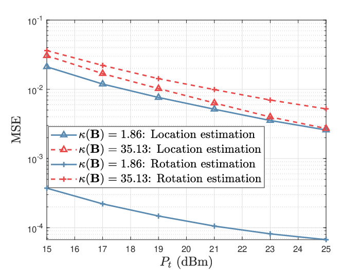
Fig. 4: MSEs of 𝐩I\mathbf{p}_{\rm I} and 𝐐\mathbf{Q} versus PtP_{t} under different values of κ⁡(𝑩)\kappa(\boldsymbol{B}).
Refer to caption
Fig. 5: MSEs of 𝐩I\mathbf{p}_{\rm I} and 𝐐\mathbf{Q} versus PtP_{t}.

In Figs. 3(a)-3(f), we evaluate the MSE performance and CRBs on the angle parameters in 𝒜\mathcal{A} versus the transmit power PtP_{t}, respectively, where the Rician factors of all related channels are set to infinity to better evaluate the accuracy of the proposed estimators. It is observed that the CRBs on all parameters decrease exponentially while increasing the transmit power. In particular, the MSEs by the proposed tensor-based method are observed to be close to the CRBs in the high transmit power regime, which thus validates its efficacy. Furthermore, in Figs. 3(g)-3(h), we plot the MSEs by the proposed 6D information acquisition scheme and the CRBs on the IRS’s location 𝐩I\mathbf{p}_{\rm I} and orientation 𝐐\mathbf{Q} (see (63) and (64)) versus the transmit power PtP_{t}. It is observed that the achieved MSEs decrease with PtP_{t}, similarly as the observations made in Figs. 3(a)-3(f) for angle parameters. It is also observed that the performance gap between the achieved MSE and CRB on 𝐐\mathbf{Q} in Fig. 3(h) is larger than that on 𝐩I\mathbf{p}_{\rm I} in Fig. 3(g). This is because the orientation estimation relies on both the estimated location 𝐩^I\mathbf{\hat{p}}_{\rm I} and angle parameters {η^ke,η^ka}k=1K\{\hat{\eta}_{k}^{e},\hat{\eta}_{k}^{a}\}_{k=1}^{K}, which may be subject to accumulated estimation error as compared to the location estimation.

Next, to verify the sensitivity results in Section V-B, we evaluate the effect of the condition number κ⁡(𝑩)\kappa(\boldsymbol{B}) on the accuracy of orientation estimation, where we set K=3K=3 with 𝐩RX,3=[−46,6,10]T\mathbf{p}_{\rm RX,3}=[-46,6,10]^{T}, and consider two different IRS locations, namely, 𝐩I=[5,4,10]T\mathbf{p}_{\rm I}=[5,4,10]^{T} and 𝐩I=[−5,−10,4]T\mathbf{p}_{\rm I}=[-5,-10,4]^{T}. With these two IRS locations, we have κ⁡(𝑩)=1.86\kappa(\boldsymbol{B})=1.86 and 35.1335.13, respectively. Fig. 5 plots the MSEs of location estimation and orientation estimation versus the transmit power PtP_{t} under the above two IRS locations. It is observed that although the performance of location estimation is similar under these two locations, the performance of orientation estimation shows significant differences. In particular, the accuracy of orientation estimation under κ⁡(𝑩)=1.86\kappa(\boldsymbol{B})=1.86 is observed to be much higher than that under κ⁡(𝑩)=35.13\kappa(\boldsymbol{B})=35.13. This implies that κ⁡(𝑩)\kappa(\boldsymbol{B}) or the location of all nodes can dramatically affect the orientation estimation even if with a small MSE in location estimation, which is consistent with our theoretical analysis in Section V-B.

VI-B Performance of 6D Information Acquisition

Since the orientation estimation relies on both the estimated location 𝐩^I\mathbf{\hat{p}}_{\rm I} and angle parameters {η^ke,η^ka}k=1K\{\hat{\eta}_{k}^{e},\hat{\eta}_{k}^{a}\}_{k=1}^{K}, to analyze their respective effects on the accuracy of orientation estimation, we compare the MSEs of orientation estimation in the following three cases, i.e.,

  • •

    Case 1: orientation estimation with estimated location and angle parameters (𝐩^I\mathbf{\hat{p}}_{\rm I} and {η^ke,η^ka}k=1K\{\hat{\eta}_{k}^{e},\hat{\eta}_{k}^{a}\}_{k=1}^{K}),

  • •

    Case 2: orientation estimation with estimated/perfect location information/angle parameters (𝐩^I\mathbf{\hat{p}}_{\rm I} and {ηke,ηka}k=1K\{{\eta}_{k}^{e},{\eta}_{k}^{a}\}_{k=1}^{K}),

  • •

    Case 3: orientation estimation with perfect/estimated location information/angle parameters (𝐩I\mathbf{p}_{\rm I} and {η^ke,η^ka}k=1K\{\hat{\eta}_{k}^{e},\hat{\eta}_{k}^{a}\}_{k=1}^{K}).

In Fig. 5, we plot the MSEs of location and orientation estimation under the above three cases versus the transmit power PtP_{t} with Mx=My=8M_{x}=M_{y}=8. It is interesting to observe that the MSE in Case 2 is lower than that in Case 3, which implies that the orientation estimation is more sensitive to the estimation error of the angle parameters {ηke,ηka}k=1K\{{\eta}_{k}^{e},{\eta}_{k}^{a}\}_{k=1}^{K} than that of the location 𝐩I\mathbf{p}_{\rm I}, which validates the analysis at the end of Section V-B. An intuitive explanation is that even a moderate deviation from the actual IRS location 𝐩I\mathbf{p}_{\rm I} (e.g., several meters) is much smaller as compared to the TX-IRS and IRS-RX kk distances, thus marginally affecting the orientation estimation; in contrast, a small deviation from the true angle parameters {ηke,ηka}k=1K\{{\eta}_{k}^{e},{\eta}_{k}^{a}\}_{k=1}^{K} can significantly alter the estimate of the rotation matrix.

Refer to caption
Fig. 6: MSEs of 𝐩I\mathbf{p}_{\rm I} and 𝐐\mathbf{Q} versus M0M_{0}.
Refer to caption
Fig. 7: MSEs of 𝐩I\mathbf{p}_{\rm I} and 𝐐\mathbf{Q} versus KK.

Next, Fig. 7 shows the performance of the proposed methods versus the number of IRS reflecting elements in each dimension, with Mx=My≜M0M_{x}=M_{y}\triangleq M_{0}. It is observed that all MSEs decrease monotonically with increasing M0M_{0}. This is because increasing M0M_{0} helps boost the received signal power at each RX, thus improving the performance of angle estimation. Moreover, it can be seen that the MSE in Case 2 approaches that in Case 1 as M0M_{0} increases. The reason is that increasing M0M_{0} helps improve the estimation accuracy of the cascaded spatial frequencies {ηke,ηka}k=1K\{{\eta}_{k}^{e},{\eta}_{k}^{a}\}_{k=1}^{K}. Moreover, the MSE in Case 3 becomes lower than that in Case 2 when M0M_{0} increases, which implies that the location estimation error may become a bottleneck to improve the orientation estimation accuracy even if the angle parameters {ηke,ηka}k=1K\{{\eta}_{k}^{e},{\eta}_{k}^{a}\}_{k=1}^{K} are accurately estimated with increasing M0M_{0}.

Finally, in Fig. 7, we show the MSEs of the location and orientation estimation versus the number of RXs, KK, with Pt=20P_{t}=20 dBm. The locations of RXs 3-6 are set to 𝐩RX,3=[−46,6,10]T\mathbf{p}_{\rm RX,3}=[-46,6,10]^{T}, 𝐩RX,4=[−2,38,3]T\mathbf{p}_{\rm RX,4}=[-2,38,3]^{T}, 𝐩RX,5=[20,−17,19]T\mathbf{p}_{\rm RX,5}=[20,-17,19]^{T}, and 𝐩RX,6=[5,10,11]T\mathbf{p}_{\rm RX,6}=[5,10,11]^{T}, respectively. It is observed that the MSE of location estimation decreases with KK, thanks to the more observations collected. Moreover, although the MSE of orientation estimation decreases with KK over the whole range in Cases 2, it is observed to be approximately constant when K>3K>3 in Cases 1 and 3. This implies that in contrast to the location estimation, the accuracy of angle parameter estimation may not improve as KK increases. This is because each RX kk independently estimates its angle parameters ηke{\eta}_{k}^{e} and ηka{\eta}_{k}^{a}, and hence the resulting angle estimation accuracy is regardless of the total number of RXs.

VII Conclusion

This paper proposes a new device-free sensing system for joint location and orientation estimation enabled by a target-mounted IRS. To this end, we first propose a tensor-based method to acquire essential angle information between the IRS and the sensing TX, as well as a set of sensing RXs, based on which the location and orientation of the IRS/target are efficiently estimated by solving two least-square problems, respectively. Theoretical analysis is provided to derive the CRBs on the involved parameters and unveil the non-trivial impacts of the locations of the sensing TX and RXs, as well as the estimation accuracy of the IRS’s cascaded spatial frequencies on the orientation estimation accuracy. In particular, the orientation estimation accuracy is shown to be very robust against the estimation error in the IRS’s location. Simulation results validate the above analytic results and demonstrate the efficacy of the proposed sensing scheme even when the number of sensing RXs is small. There are several promising directions worthy of further investigation for the proposed target-mounted IRS-assisted sensing in future work, such as its applications for multi-target sensing, target recognition and tracking, integrated sensing and communication (ISAC), etc.

\useRomanappendicesfalse

Appendix A Calculation of FIM 𝑰⁡(𝚪)\boldsymbol{I}(\boldsymbol{\Gamma})

Based on (28), the log-likelihood function of the parameter vector 𝚪\boldsymbol{\Gamma} in (61) can be expressed as

ℒ⁡(𝚪)=\displaystyle\mathcal{L}(\boldsymbol{\Gamma})= −D~−1σ2​∑k=1K‖𝒀k,(1)−𝒂~r,k​(𝒂~I,k⊙𝒂~t)T‖F2,\displaystyle-\tilde{D}-\frac{1}{\sigma^{2}}\sum_{k=1}^{K}\|\boldsymbol{Y}_{k,(1)}-\boldsymbol{\tilde{a}}_{r,k}(\boldsymbol{\tilde{a}}_{I,k}\odot\boldsymbol{\tilde{a}}_{t})^{T}\|_{F}^{2},
=\displaystyle= −D~−1σ2​∑k=1K‖𝒀k,(2)−𝒂~t​(𝒂~I,k⊙𝒂~r,k)T‖F2,\displaystyle-\tilde{D}-\frac{1}{\sigma^{2}}\sum_{k=1}^{K}\|\boldsymbol{Y}_{k,(2)}-\boldsymbol{\tilde{a}}_{t}(\boldsymbol{\tilde{a}}_{I,k}\odot\boldsymbol{\tilde{a}}_{r,k})^{T}\|_{F}^{2},
=\displaystyle= −D~−1σ2​∑k=1K‖𝒀k,(3)−𝒂~I,k​(𝒂~t⊙𝒂~r,k)T‖F2,\displaystyle-\tilde{D}-\frac{1}{\sigma^{2}}\sum_{k=1}^{K}\|\boldsymbol{Y}_{k,(3)}-\boldsymbol{\tilde{a}}_{I,k}(\boldsymbol{\tilde{a}}_{t}\odot\boldsymbol{\tilde{a}}_{r,k})^{T}\|_{F}^{2}, (73)

where D~≜DRe​DBS​DIRS​K​ln⁡π​σ2\tilde{D}\triangleq D_{\rm Re}D_{\rm BS}D_{\rm IRS}K\ln\pi\sigma^{2}. Then, the FIM for 𝚪\boldsymbol{\Gamma} is given by 𝑰⁡(𝚪)=𝔼⁡{(∂ℒ⁡(𝚪)∂𝚪)T​∂ℒ⁡(𝚪)∂𝚪}\boldsymbol{I}(\boldsymbol{\Gamma})=\mathbb{E}\left\{\left(\frac{\partial\mathcal{L}(\boldsymbol{\Gamma})}{\partial\boldsymbol{\Gamma}}\right)^{T}\frac{\partial\mathcal{L}(\boldsymbol{\Gamma})}{\partial\boldsymbol{\Gamma}}\right\}[24, 18]. To calculate 𝑰⁡(𝚪)\boldsymbol{I}(\boldsymbol{\Gamma}), we first compute the partial derivative of ℒ⁡(𝚪)\mathcal{L}(\boldsymbol{\Gamma}) w.r.t. 𝚪\boldsymbol{\Gamma} and then calculate its expectation, as presented in the subsequent two subsections, respectively.

A-A Partial Derivatives of ℒ⁡(𝚪)\mathcal{L}(\boldsymbol{\Gamma}) w.r.t. 𝚪\boldsymbol{\Gamma}

First, the partial derivative of ℒ⁡(𝚪)\mathcal{L}(\boldsymbol{\Gamma}) w.r.t. ζ0a\zeta_{0}^{a} can be calculated as

∂ℒ⁡(𝚪)∂ζ0a=tr⁡{(∂ℒ⁡(𝚪)∂𝒂~t)T​∂𝒂~t∂ζ0a+(∂ℒ⁡(𝚪)∂𝒂~t∗)T​∂𝒂~t∗∂ζ0a},\displaystyle\frac{\partial\mathcal{L}(\boldsymbol{\Gamma})}{\partial\zeta_{0}^{a}}={\rm tr}\left\{\left(\frac{\partial\mathcal{L}(\boldsymbol{\Gamma})}{\partial\boldsymbol{\tilde{a}}_{t}}\right)^{T}\frac{\partial\boldsymbol{\tilde{a}}_{t}}{\partial\zeta_{0}^{a}}+\left(\frac{\partial\mathcal{L}(\boldsymbol{\Gamma})}{\partial\boldsymbol{\tilde{a}}_{t}^{\ast}}\right)^{T}\frac{\partial\boldsymbol{\tilde{a}}_{t}^{\ast}}{\partial\zeta_{0}^{a}}\right\}, (74)

where

∂ℒ⁡(𝚪)∂𝒂~t=(∂ℒ⁡(𝚪)∂𝒂~t∗)∗=1σ2​∑k=1K(𝒀k,(2)T−(𝒂~I,k⊙𝒂~r,k)​𝒂~tT)H​(𝒂~I,k⊙𝒂~r,k)\displaystyle\frac{\partial\mathcal{L}(\boldsymbol{\Gamma})}{\partial\boldsymbol{\tilde{a}}_{t}}=\left(\frac{\partial\mathcal{L}(\boldsymbol{\Gamma})}{\partial\boldsymbol{\tilde{a}}_{t}^{\ast}}\right)^{\ast}=\frac{1}{\sigma^{2}}\sum_{k=1}^{K}\left(\boldsymbol{Y}_{k,(2)}^{T}-(\boldsymbol{\tilde{a}}_{I,k}\odot\boldsymbol{\tilde{a}}_{r,k})\boldsymbol{\tilde{a}}_{t}^{T}\right)^{H}\left(\boldsymbol{\tilde{a}}_{I,k}\odot\boldsymbol{\tilde{a}}_{r,k}\right)
∂𝒂~t∂ζ0a=(∂𝒂~t∗∂ζ0a)∗=−j​𝑭T​𝑫a​(Nty,Ntz)​𝒂t∗​(ζ0e,ζ0a),\displaystyle\frac{\partial\boldsymbol{\tilde{a}}_{t}}{\partial\zeta_{0}^{a}}=\left(\frac{\partial\boldsymbol{\tilde{a}}_{t}^{\ast}}{\partial\zeta_{0}^{a}}\right)^{\ast}=-j\boldsymbol{F}^{T}\boldsymbol{D}_{a}(N_{t_{y}},N_{t_{z}})\boldsymbol{a}_{t}^{\ast}(\zeta_{0}^{e},\zeta_{0}^{a}),
𝑫a​(N1,N2)=π​diag​([0,1,…,N1−1]T⊗𝟏N2).\displaystyle\boldsymbol{D}_{a}(N_{1},N_{2})=\pi{\rm diag}\big([0,1,\ldots,N_{1}-1]^{T}\otimes\boldsymbol{1}_{N_{2}}\big). (75)

By performing some manipulations on (74), it can be simplified as ∂ℒ⁡(𝚪)∂ζ0a=2σ2​∑k=1Kℜ⁡{(𝒂~I,k⊙𝒂~r,k)T​(𝒀k,(2)T−(𝒂~I,k⊙𝒂~r,k)​𝒂~tT)∗​∂𝒂~t∂ζ0a}\frac{\partial\mathcal{L}(\boldsymbol{\Gamma})}{\partial\zeta_{0}^{a}}=\frac{2}{\sigma^{2}}\sum_{k=1}^{K}\Re\{(\boldsymbol{\tilde{a}}_{I,k}\odot\boldsymbol{\tilde{a}}_{r,k})^{T}(\boldsymbol{Y}_{k,(2)}^{T}-(\boldsymbol{\tilde{a}}_{I,k}\odot\boldsymbol{\tilde{a}}_{r,k})\boldsymbol{\tilde{a}}_{t}^{T})^{\ast}\frac{\partial\boldsymbol{\tilde{a}}_{t}}{\partial\zeta_{0}^{a}}\}. Similarly, we can obtain the partial derivatives w.r.t. the other angle parameters as follows,

∂ℒ⁡(𝚪)∂ζ0e=2σ2​∑k=1Kℜ⁡{(𝒂~I,k⊙𝒂~r,k)T​(𝒀k,(2)T−(𝒂~I,k⊙𝒂~r,k)​𝒂~tT)∗​∂𝒂~t∂ζ0e},\displaystyle\frac{\partial\mathcal{L}(\boldsymbol{\Gamma})}{\partial\zeta_{0}^{e}}=\frac{2}{\sigma^{2}}\sum_{k=1}^{K}\Re\left\{\left(\boldsymbol{\tilde{a}}_{I,k}\odot\boldsymbol{\tilde{a}}_{r,k}\right)^{T}\left(\boldsymbol{Y}_{k,(2)}^{T}-(\boldsymbol{\tilde{a}}_{I,k}\odot\boldsymbol{\tilde{a}}_{r,k})\boldsymbol{\tilde{a}}_{t}^{T}\right)^{\ast}\frac{\partial\boldsymbol{\tilde{a}}_{t}}{\partial\zeta_{0}^{e}}\right\}, (76)
∂ℒ⁡(𝚪)∂ζka=2σ2​ℜ⁡{(𝒂~I,k⊙𝒂~t)T​(𝒀k,(1)T−(𝒂~I,k⊙𝒂~t)​𝒂~r,kT)∗​∂𝒂~r,k∂ζa},\displaystyle\frac{\partial\mathcal{L}(\boldsymbol{\Gamma})}{\partial\zeta_{k}^{a}}=\frac{2}{\sigma^{2}}\Re\left\{\left(\boldsymbol{\tilde{a}}_{I,k}\odot\boldsymbol{\tilde{a}}_{t}\right)^{T}\left(\boldsymbol{Y}_{k,(1)}^{T}-(\boldsymbol{\tilde{a}}_{I,k}\odot\boldsymbol{\tilde{a}}_{t})\boldsymbol{\tilde{a}}_{r,k}^{T}\right)^{\ast}\frac{\partial\boldsymbol{\tilde{a}}_{r,k}}{\partial\zeta^{a}}\right\}, (77)
∂ℒ⁡(𝚪)∂ζke=2σ2​ℜ⁡{(𝒂~I,k⊙𝒂~t)T​(𝒀k,(1)T−(𝒂~I,k⊙𝒂~t)​𝒂~r,kT)∗​∂𝒂~r,k∂ζa},\displaystyle\frac{\partial\mathcal{L}(\boldsymbol{\Gamma})}{\partial\zeta_{k}^{e}}=\frac{2}{\sigma^{2}}\Re\left\{\left(\boldsymbol{\tilde{a}}_{I,k}\odot\boldsymbol{\tilde{a}}_{t}\right)^{T}\left(\boldsymbol{Y}_{k,(1)}^{T}-(\boldsymbol{\tilde{a}}_{I,k}\odot\boldsymbol{\tilde{a}}_{t})\boldsymbol{\tilde{a}}_{r,k}^{T}\right)^{\ast}\frac{\partial\boldsymbol{\tilde{a}}_{r,k}}{\partial\zeta^{a}}\right\}, (78)
∂ℒ⁡(𝚪)∂ηka=2σ2​ℜ⁡{(𝒂~t⊙𝒂~r,k)T​(𝒀k,(3)T−(𝒂~t⊙𝒂~r,k)​𝒂~I,kT)∗​∂𝒂~I,k∂ηka},\displaystyle\frac{\partial\mathcal{L}(\boldsymbol{\Gamma})}{\partial\eta_{k}^{a}}=\frac{2}{\sigma^{2}}\Re\left\{\left(\boldsymbol{\tilde{a}}_{t}\odot\boldsymbol{\tilde{a}}_{r,k}\right)^{T}\left(\boldsymbol{Y}_{k,(3)}^{T}-(\boldsymbol{\tilde{a}}_{t}\odot\boldsymbol{\tilde{a}}_{r,k})\boldsymbol{\tilde{a}}_{I,k}^{T}\right)^{\ast}\frac{\partial\boldsymbol{\tilde{a}}_{I,k}}{\partial\eta_{k}^{a}}\right\}, (79)
∂ℒ⁡(𝚪)∂ηke=2σ2​ℜ⁡{(𝒂~t⊙𝒂~r,k)T​(𝒀k,(3)T−(𝒂~t⊙𝒂~r,k)​𝒂~I,kT)∗​∂𝒂~I,k∂ηke},\displaystyle\frac{\partial\mathcal{L}(\boldsymbol{\Gamma})}{\partial\eta_{k}^{e}}=\frac{2}{\sigma^{2}}\Re\left\{\left(\boldsymbol{\tilde{a}}_{t}\odot\boldsymbol{\tilde{a}}_{r,k}\right)^{T}\left(\boldsymbol{Y}_{k,(3)}^{T}-(\boldsymbol{\tilde{a}}_{t}\odot\boldsymbol{\tilde{a}}_{r,k})\boldsymbol{\tilde{a}}_{I,k}^{T}\right)^{\ast}\frac{\partial\boldsymbol{\tilde{a}}_{I,k}}{\partial\eta_{k}^{e}}\right\}, (80)

where

∂𝒂~t∂ζ0e=\displaystyle\frac{\partial\boldsymbol{\tilde{a}}_{t}}{\partial\zeta_{0}^{e}}= (−j​𝑭T​𝑫e​(Ntx,Nty)​𝒂t∗​(ζ0e,ζ0a)),∂𝒂~r,k∂ζka=j​𝑾kH​𝑫a​(Nry,Nrz)​𝒂r​(ζke,ζka),\displaystyle\left(-j\boldsymbol{F}^{T}\boldsymbol{D}_{e}(N_{t_{x}},N_{t_{y}})\boldsymbol{a}_{t}^{\ast}(\zeta_{0}^{e},\zeta_{0}^{a})\right),\frac{\partial\boldsymbol{\tilde{a}}_{r,k}}{\partial\zeta_{k}^{a}}=j\boldsymbol{W}_{k}^{H}\boldsymbol{D}_{a}(N_{r_{y}},N_{r_{z}})\boldsymbol{a}_{r}({\zeta}_{k}^{e},\zeta_{k}^{a}),
∂𝒂~r,k∂ζke=\displaystyle\frac{\partial\boldsymbol{\tilde{a}}_{r,k}}{\partial\zeta_{k}^{e}}= j​𝑾kH​𝑫e​(Nry,Nrz)​𝒂r​(ζke,ζka),∂𝒂~r,k∂ηka=j​𝑽H​𝑫a​(Mx,My)​𝒂I​(ηke,ηka),\displaystyle j\boldsymbol{W}_{k}^{H}\boldsymbol{D}_{e}(N_{r_{y}},N_{r_{z}})\boldsymbol{a}_{r}({\zeta}_{k}^{e},\zeta_{k}^{a}),\frac{\partial\boldsymbol{\tilde{a}}_{r,k}}{\partial\eta_{k}^{a}}=j\boldsymbol{V}^{H}\boldsymbol{D}_{a}(M_{x},M_{y})\boldsymbol{a}_{I}({\eta}_{k}^{e},\eta_{k}^{a}),
∂𝒂~r,k∂ηke=\displaystyle\frac{\partial\boldsymbol{\tilde{a}}_{r,k}}{\partial\eta_{k}^{e}}= j​𝑽H​𝑫e​(Mx,My)​𝒂I​(ηke,ηka),𝑫e​(N1,N2)=π​diag​(𝟏N1⊗[0,1,…,N2−1]T).\displaystyle j\boldsymbol{V}^{H}\boldsymbol{D}_{e}(M_{x},M_{y})\boldsymbol{a}_{I}({\eta}_{k}^{e},\eta_{k}^{a}),\boldsymbol{D}_{e}(N_{1},N_{2})=\pi{\rm diag}(\boldsymbol{1}_{N_{1}}\otimes[0,1,\ldots,N_{2}-1]^{T}). (81)

A-B Calculation of FIM 𝐈⁡(𝚪)\boldsymbol{I}(\boldsymbol{\Gamma})

To calculate the FIM 𝑰⁡(𝚪)\boldsymbol{I}(\boldsymbol{\Gamma}), we start from its diagonal and subdiagonal entries. Due to the tedious calculations for all these entries and space limit, we only show the details for some of them. For example, the (1,1)(1,1)-th or the first diagonal element of 𝑰⁡(𝚪)\boldsymbol{I}(\boldsymbol{\Gamma}) is given by 𝔼⁡{(∂ℒ⁡(𝚪)∂ζ0a)∗​∂ℒ⁡(𝚪)∂ζ0a}=4​𝔼​[ℜ⁡{c¯0,a}2]\mathbb{E}\left\{\left(\frac{\partial\mathcal{L}(\boldsymbol{\Gamma})}{\partial\zeta_{0}^{a}}\right)^{\ast}\frac{\partial\mathcal{L}(\boldsymbol{\Gamma})}{\partial\zeta_{0}^{a}}\right\}=4\mathbb{E}\left[\Re\{\bar{c}_{0,a}\}^{2}\right], where

c¯0,a≜\displaystyle\bar{c}_{0,a}\triangleq ∑k=1K1σ2​(𝒂~I,k⊙𝒂~r,k)T​(𝒀k,(2)T−(𝒂~I,k⊙𝒂~r,k)​𝒂~tT)∗​∂𝒂~t∂ζ0a=1σ2​∑k=1K(𝒂~I,k⊙𝒂~r,k)T​𝑵k,(2)H​∂𝒂~t∂ζ0a\displaystyle\sum_{k=1}^{K}\frac{1}{\sigma^{2}}\left(\boldsymbol{\tilde{a}}_{I,k}\odot\boldsymbol{\tilde{a}}_{r,k}\right)^{T}\left(\boldsymbol{Y}_{k,(2)}^{T}-(\boldsymbol{\tilde{a}}_{I,k}\odot\boldsymbol{\tilde{a}}_{r,k})\boldsymbol{\tilde{a}}_{t}^{T}\right)^{\ast}\frac{\partial\boldsymbol{\tilde{a}}_{t}}{\partial\zeta_{0}^{a}}=\frac{1}{\sigma^{2}}\sum_{k=1}^{K}\left(\boldsymbol{\tilde{a}}_{I,k}\odot\boldsymbol{\tilde{a}}_{r,k}\right)^{T}\boldsymbol{N}_{k,(2)}^{H}\frac{\partial\boldsymbol{\tilde{a}}_{t}}{\partial\zeta_{0}^{a}}
=\displaystyle= 1σ2​∑k=1K((∂𝒂~t∂ζ0a)T⊗(𝒂~I,k⊙𝒂~r,k)T)​vec​(𝑵k,(2)H)=1σ2​∑k=1K𝒖¯k,aT​𝒏k,(2),\displaystyle\frac{1}{\sigma^{2}}\sum_{k=1}^{K}\left(\left(\frac{\partial\boldsymbol{\tilde{a}}_{t}}{\partial\zeta_{0}^{a}}\right)^{T}\otimes\left(\boldsymbol{\tilde{a}}_{I,k}\odot\boldsymbol{\tilde{a}}_{r,k}\right)^{T}\right){\rm vec}\left(\boldsymbol{N}_{k,(2)}^{H}\right)=\frac{1}{\sigma^{2}}\sum_{k=1}^{K}\boldsymbol{\bar{u}}_{k,a}^{T}\boldsymbol{n}_{k,(2)}, (82)

with 𝒖¯k,aT≜(∂𝒂~t∂ζ0a)T⊗(𝒂~I,k⊙𝒂~r,k)T\boldsymbol{\bar{u}}_{k,a}^{T}\triangleq\left(\frac{\partial\boldsymbol{\tilde{a}}_{t}}{\partial\zeta_{0}^{a}}\right)^{T}\otimes(\boldsymbol{\tilde{a}}_{I,k}\odot\boldsymbol{\tilde{a}}_{r,k})^{T} and 𝒏k,(2)≜vec⁡(𝑵k,(2)H)\boldsymbol{n}_{k,(2)}\triangleq{\rm vec}\left(\boldsymbol{N}_{k,(2)}^{H}\right). It follows from (82) that c0,ac_{0,a} is the linear transformation of 𝒏k,(2)\boldsymbol{n}_{k,(2)} and follows the CSCG distribution. As the effective received noises at different RXs are mutually independent, their variance and second-order moments are given by 𝔼⁡(c¯0,a​c¯0,a∗)=1σ2​∑k=1K𝒖¯k,aT​𝒖¯k,a∗\mathbb{E}(\bar{c}_{0,a}\bar{c}_{0,a}^{\ast})=\frac{1}{\sigma^{2}}\sum_{k=1}^{K}\boldsymbol{\bar{u}}_{k,a}^{T}\boldsymbol{\bar{u}}_{k,a}^{\ast} and 𝔼⁡(c¯0,a​c¯0,a)=0\mathbb{E}(\bar{c}_{0,a}\bar{c}_{0,a})=0, respectively, which result in

𝔼⁡{(∂ℒ⁡(𝚪)∂ζ0a)∗​∂ℒ⁡(𝚪)∂ζ0a}=2σ2​∑k=1K𝒖¯k,aT​𝒖¯k,a∗.\displaystyle\mathbb{E}\left\{\left(\frac{\partial\mathcal{L}(\boldsymbol{\Gamma})}{\partial\zeta_{0}^{a}}\right)^{\ast}\frac{\partial\mathcal{L}(\boldsymbol{\Gamma})}{\partial\zeta_{0}^{a}}\right\}=\frac{2}{\sigma^{2}}\sum_{k=1}^{K}\boldsymbol{\bar{u}}_{k,a}^{T}\boldsymbol{\bar{u}}_{k,a}^{\ast}. (83)

For the (1,2)(1,2)-th or the first subdiagonal element of 𝑰⁡(𝚪)\boldsymbol{I}(\boldsymbol{\Gamma}), it can be calculated as 𝔼⁡{(∂ℒ⁡(𝚪)∂ζ0a)∗​∂ℒ⁡(𝚪)∂ζ0e}=2σ2​∑k=1Kℜ⁡(𝒖¯k,aT​𝒖¯k,e∗)\mathbb{E}\big\{(\frac{\partial\mathcal{L}(\boldsymbol{\Gamma})}{\partial\zeta_{0}^{a}})^{\ast}\frac{\partial\mathcal{L}(\boldsymbol{\Gamma})}{\partial\zeta_{0}^{e}}\big\}=\frac{2}{\sigma^{2}}\sum_{k=1}^{K}\Re\big(\boldsymbol{\bar{u}}_{k,a}^{T}\boldsymbol{\bar{u}}_{k,e}^{\ast}\big), where 𝒖¯k,eT≜(∂𝒂~t∂ζ0e)T⊗(𝒂~I,k⊙𝒂~r,k)T\boldsymbol{\bar{u}}_{k,e}^{T}\triangleq\left(\frac{\partial\boldsymbol{\tilde{a}}_{t}}{\partial\zeta_{0}^{e}}\right)^{T}\otimes\left(\boldsymbol{\tilde{a}}_{I,k}\odot\boldsymbol{\tilde{a}}_{r,k}\right)^{T}. Following the same procedure, we can obtain all (i,i)(i,i)-th (diagonal) and (i,i+1)(i,i+1)-th (subdiagonal) elements, for which the details are omitted.

Next, we derive the expressions of the off-diagonal entries of 𝑰⁡(𝚪)\boldsymbol{I}(\boldsymbol{\Gamma}). Similarly, we only show the expressions for partial off-diagonal entries. For example, the (1,k+2)(1,k+2)-th element of 𝑰⁡(𝚪)\boldsymbol{I}(\boldsymbol{\Gamma}) is given by

𝔼⁡{(∂ℒ⁡(𝚪)∂ζ0a)∗​∂ℒ⁡(𝚪)∂ζka}=𝔼⁡((c¯0,a+c¯0,a∗)​(ck,a+ck,a∗)),\displaystyle\mathbb{E}\left\{\left(\frac{\partial\mathcal{L}(\boldsymbol{\Gamma})}{\partial\zeta_{0}^{a}}\right)^{\ast}\frac{\partial\mathcal{L}(\boldsymbol{\Gamma})}{\partial\zeta_{k}^{a}}\right\}=\mathbb{E}((\bar{c}_{0,a}+\bar{c}_{0,a}^{\ast})(c_{k,a}+c_{k,a}^{\ast})), (84)

where c¯0,a\bar{c}_{0,a} is defined in (82) and ck,a≜1σ2​𝒖k,aT​𝒏k,(1)c_{k,a}\triangleq\frac{1}{\sigma^{2}}\boldsymbol{u}_{k,a}^{T}\boldsymbol{n}_{k,(1)} with 𝒏k,(1)=vec⁡(𝑵k,(1)H)\boldsymbol{n}_{k,(1)}={\rm vec}\left(\boldsymbol{N}_{k,(1)}^{H}\right). It follows from (83) that their second-order moments are given by 𝔼⁡(c¯0,a​ck,a)=0\mathbb{E}(\bar{c}_{0,a}c_{k,a})=0, whilst their correlation can be calculated as

𝔼⁡(c¯0,a​ck,a∗)=\displaystyle\mathbb{E}(\bar{c}_{0,a}c_{k,a}^{\ast})= 1σ4​𝔼​{∑i=1K𝒖¯i,aT​𝒏i,(2)​𝒏k,(1)H​𝒖k,a∗}=(a)1σ4​𝒖¯k,aT​𝔼​(𝒏k,(2)​𝒏k,(1)H)​𝒖k,a∗=1σ4​𝒖¯k,aT​𝑪2,1​𝒖k,a∗,\displaystyle\frac{1}{\sigma^{4}}\mathbb{E}\left\{\sum_{i=1}^{K}\boldsymbol{\bar{u}}_{i,a}^{T}\boldsymbol{n}_{i,(2)}\boldsymbol{n}_{k,(1)}^{H}\boldsymbol{u}_{k,a}^{\ast}\right\}\stackrel{{\scriptstyle(a)}}{{=}}\frac{1}{\sigma^{4}}\boldsymbol{\bar{u}}_{k,a}^{T}\mathbb{E}(\boldsymbol{n}_{k,(2)}\boldsymbol{n}_{k,(1)}^{H})\boldsymbol{u}_{k,a}^{\ast}=\frac{1}{\sigma^{4}}\boldsymbol{\bar{u}}_{k,a}^{T}\boldsymbol{C}_{2,1}\boldsymbol{u}_{k,a}^{\ast},

where in (a)(a) we use the property that the received noise at different RXs is independent of each other, and 𝑪2,1≜E⁡(𝒏k,(2)​𝒏k,(1)H).\boldsymbol{C}_{2,1}\triangleq E(\boldsymbol{n}_{k,(2)}\boldsymbol{n}_{k,(1)}^{H}). Therefore, (84) becomes 𝔼⁡{(∂ℒ⁡(𝚪)∂ζ0a)∗​∂ℒ⁡(𝚪)∂ζka}=2σ4​ℜ⁡{𝒖¯k,aT​𝑪2,1​𝒖k,a∗}.\mathbb{E}\{(\frac{\partial\mathcal{L}(\boldsymbol{\Gamma})}{\partial\zeta_{0}^{a}})^{\ast}\frac{\partial\mathcal{L}(\boldsymbol{\Gamma})}{\partial\zeta_{k}^{a}}\}=\frac{2}{\sigma^{4}}\Re\{\boldsymbol{\bar{u}}_{k,a}^{T}\boldsymbol{C}_{2,1}\boldsymbol{u}_{k,a}^{\ast}\}. Next, we compute 𝑪2,1\boldsymbol{C}_{2,1} in the above fomula. Since the entries in 𝓝k\boldsymbol{\mathcal{N}}_{k} are all i.i.d. Gaussian random variables, we have

𝔼⁡(nk,i1,j1,q1​nk,i2,j2,q2∗)={σ2,if i1=i2,j1=j2,q1=q2,0,otherwise.\displaystyle\mathbb{E}(n_{k,{i_{1},j_{1},q_{1}}}n_{k,{i_{2},j_{2},q_{2}}}^{\ast})=\begin{cases}\sigma^{2},&{\text{if }}i_{1}=i_{2},j_{1}=j_{2},q_{1}=q_{2},\\ 0,&{\text{otherwise}.}\end{cases} (85)

Hence, there should exist DRX​DBS​DIRSD_{\rm RX}D_{\rm BS}D_{\rm IRS} nonzero entries in the correlation matrices 𝑪2,1\boldsymbol{C}_{2,1}, and its (m,n)(m,n)-th element, based on the relationship between 𝓝k\boldsymbol{{\mathcal{N}}}_{k} and 𝑵k,(1)\boldsymbol{N}_{k,(1)}/𝑵k,(2)\boldsymbol{N}_{k,(2)}, is expressed as

𝑪2,1​[m,n]={σ2,if m=M2(i,j,q),n=M1(i,j,q),0,otherwise,\displaystyle\boldsymbol{C}_{2,1}[m,n]=\begin{cases}\sigma^{2},&{\text{if }}m=M_{2}(i,j,q),n=M_{1}(i,j,q),\\ 0,&{\text{otherwise,}}\end{cases} (86)

where M1​(i,j,q)=j+(q−1)​DTX+(i−1)​DTX​DIRSM_{1}(i,j,q)=j+(q-1)D_{\rm TX}+(i-1)D_{\rm TX}D_{\rm IRS} and M2​(i,j,q)=i+(q−1)​DRX+(j−1)​DRX​DIRS.M_{2}(i,j,q)=i+(q-1)D_{\rm RX}+(j-1)D_{\rm RX}D_{\rm IRS}. By performing similar operations as above, we can calculate the other off-diagonal elements of 𝑰⁡(𝚪)\boldsymbol{I}(\boldsymbol{\Gamma}), for which the details are omitted for brevity.

Appendix B Calculation of Jacobian Matrix ∇𝒔𝚪\nabla_{\boldsymbol{s}}\boldsymbol{\Gamma}

The (i,j)(i,j)-th element of ∇𝒔𝚪\nabla_{\boldsymbol{s}}\boldsymbol{\Gamma} is given by ∂Γ⁡[i]∂s⁡[j]\frac{\partial\Gamma[i]}{\partial s[j]}, where Γ⁡[i]\Gamma[i] is the ii-th entry of the vector 𝚪\boldsymbol{\Gamma} defined in (61) and s⁡[j]s[j] is the jj-th entry of the vector 𝐬=[𝐩IT,𝝍T]T\mathbf{s}=[\mathbf{p}_{\rm I}^{T},\boldsymbol{\psi}^{T}]^{T}. Note that the angle parameters 𝜻a\boldsymbol{\zeta}^{a} and 𝜻e\boldsymbol{\zeta}^{e} are regardless of the axis angles 𝝍\boldsymbol{\psi}, and their partial derivatives w.r.t. the location 𝐩I\mathbf{p}_{\rm I} have been provided in (44). Next, we focus on the partial derivatives of angle parameters 𝜼a\boldsymbol{\eta}^{a} and 𝜼e\boldsymbol{\eta}^{e} w.r.t. 𝐩I\mathbf{p}_{\rm I} and 𝝍\boldsymbol{\psi}, respectively.

For clarity, we rewrite ηka\eta_{k}^{a} and ηke\eta_{k}^{e} in (49) and (50) as a function of 𝐩I\mathbf{p}_{\rm I} and 𝐐\mathbf{Q}, i.e., ηka​(𝐩I,𝐐)=𝒆1T​𝐐T​𝒃k​(𝐩I)\eta^{a}_{k}(\mathbf{p}_{\rm I},\mathbf{Q})=\boldsymbol{e}_{1}^{T}\mathbf{Q}^{T}\boldsymbol{b}_{k}(\mathbf{p}_{\rm I}), and ηke​(𝐩I,𝐐)=𝒆2T​𝐐T​𝒃k​(𝐩I),∀k\eta^{e}_{k}(\mathbf{p}_{\rm I},\mathbf{Q})=\boldsymbol{e}_{2}^{T}\mathbf{Q}^{T}\boldsymbol{b}_{k}(\mathbf{p}_{\rm I}),\forall k, where 𝐛k​(𝐩I)\mathbf{b}_{k}(\mathbf{p}_{\rm I}) is defined in (51). Based on the above, the partial derivative of ηka\eta_{k}^{a} and ηke\eta_{k}^{e} w.r.t. 𝐩I\mathbf{p}_{\rm I} are given by ∂ηka​(𝐩,𝐐)∂𝐩=𝑱bk​(𝐩I)​𝐐​𝒆1\frac{\partial\eta_{k}^{a}(\mathbf{p},\mathbf{Q})}{\partial\mathbf{p}}=\boldsymbol{J}_{b_{k}}(\mathbf{p}_{\rm I})\mathbf{Q}\boldsymbol{e}_{1}, and ∂ηke​(𝐩,𝐐)∂𝐩=𝑱bk​(𝐩I)​𝐐​𝒆2\frac{\partial\eta_{k}^{e}(\mathbf{p},\mathbf{Q})}{\partial\mathbf{p}}=\boldsymbol{J}_{b_{k}}(\mathbf{p}_{\rm I})\mathbf{Q}\boldsymbol{e}_{2}, respectively, where 𝑱bk​(𝐩)\boldsymbol{J}_{b_{k}}(\mathbf{p}) is the Jacobian matrix of 𝐛k​(𝐩)\mathbf{b}_{k}(\mathbf{p}) w.r.t. 𝐩\mathbf{p}, i.e., 𝑱bk​(𝐩)=[∂𝐛k​[1]∂𝐩,∂𝐛k​[2]∂𝐩,∂𝐛k​[3]∂𝐩]∈ℝ3×3\boldsymbol{J}_{b_{k}}(\mathbf{p})=[\frac{\partial\mathbf{b}_{k}[1]}{\partial\mathbf{p}},\frac{\partial\mathbf{b}_{k}[2]}{\partial\mathbf{p}},\frac{\partial\mathbf{b}_{k}[3]}{\partial\mathbf{p}}]\in\mathbb{R}^{3\times 3}, with 𝒃k​[i]\boldsymbol{b}_{k}[i] being the ii-th entry of 𝒃k​(𝐩)\boldsymbol{b}_{k}(\mathbf{p}), i.e.,∂𝐛k​[1]∂𝐩=𝒉⁡(𝐩,𝒆1),∂𝐛k​[2]∂𝐩=𝒉⁡(𝐩,𝒆2),∂𝐛k​[3]∂𝐩=𝒉⁡(𝐩,𝒆3)\frac{\partial\mathbf{b}_{k}[1]}{\partial\mathbf{p}}=\boldsymbol{h}(\mathbf{p};\boldsymbol{e}_{1}),\frac{\partial\mathbf{b}_{k}[2]}{\partial\mathbf{p}}=\boldsymbol{h}(\mathbf{p};\boldsymbol{e}_{2}),\frac{\partial\mathbf{b}_{k}[3]}{\partial\mathbf{p}}=\boldsymbol{h}(\mathbf{p};\boldsymbol{e}_{3}), 𝒉⁡(𝐩,𝒆)=2​drλ​(𝒇⁡(𝐩,𝒆,𝐩TX)+𝒇⁡(𝐩,𝒆,𝐩RX,k)),\boldsymbol{h}(\mathbf{p};\boldsymbol{e})=\frac{2d_{r}}{\lambda}\left({\boldsymbol{f}}(\mathbf{p};\boldsymbol{e},\mathbf{p}_{\rm TX})+{\boldsymbol{f}}(\mathbf{p};\boldsymbol{e},\mathbf{p}_{{\rm RX},k})\right), and 𝒇⁡(𝐩,𝒆,𝐩k)\boldsymbol{f}(\mathbf{p};\boldsymbol{e},\mathbf{p}_{k}) being defined in (44). On the other hand, the partial derivative of ηka\eta_{k}^{a} and ηke\eta_{k}^{e} w.r.t. the axis angles ψx\psi_{x}, ψy\psi_{y}, and ψz\psi_{z} are given by ∂ηka​(𝐩,𝐐)∂ψi=𝐛kT​(𝐩)​∂𝐪1∂ψi\frac{\partial\eta_{k}^{a}(\mathbf{p},\mathbf{Q})}{\partial\psi_{i}}=\mathbf{b}_{k}^{T}(\mathbf{p})\frac{\partial\mathbf{q}_{1}}{\partial\psi_{i}}, and ∂ηke​(𝐩,𝐐)∂ψi=𝐛kT(𝐩)∂𝐪2∂ψi,i=x,y,z\frac{\partial\eta_{k}^{e}(\mathbf{p},\mathbf{Q})}{\partial\psi_{i}}=\mathbf{b}_{k}^{T}(\mathbf{p})\frac{\partial\mathbf{q}_{2}}{\partial\psi_{i}},i={x,y,z}, respectively, where 𝐪1\mathbf{q}_{1} and 𝐪2\mathbf{q}_{2} are the first and second columns of the matrix 𝐐\mathbf{Q}, respectively. Based on the above, the Jacobian matrix ∇𝒔𝚪\nabla_{\boldsymbol{s}}\boldsymbol{\Gamma} can be obtained.

Appendix C Calculation of Jacobian Matrix ∇𝒔𝐪¯\nabla_{\boldsymbol{s}}\boldsymbol{\mathbf{\bar{q}}}

The (i,j)(i,j)-th element of ∇𝒔𝐪¯\nabla_{\boldsymbol{s}}\mathbf{\bar{q}} is given by ∂q¯​[i]∂s⁡[j]\frac{\partial\bar{\rm q}[i]}{\partial s[j]}, where q¯​[i]\bar{\rm q}[i] is the ii-th entry of the vector 𝐪¯=vec⁡(𝐐)\mathbf{\bar{q}}={\rm vec}(\mathbf{Q}) and s⁡[j]s[j] is the jj-th entry of the vector 𝐬=[𝐩IT,𝝍T]T\mathbf{s}=[\mathbf{p}_{\rm I}^{T},\boldsymbol{\psi}^{T}]^{T}. As shown in (1), the rotation matrix 𝐐\mathbf{Q} is regardless of the IRS location 𝐩I\mathbf{p}_{\rm I}. Hence, we only need to derive its partial derivative w.r.t. 𝝍\boldsymbol{\psi}. For example, the first entry of 𝐪¯\mathbf{\bar{q}} is given by q¯[1]=cosψycosψz,\bar{q}[1]=\cos\psi_{y}\cos\psi_{z}, and its partial derivative w.r.t. 𝝍\boldsymbol{\psi} can be calculated as ∂q¯​[1]∂𝝍=[0,−sinψycosψz,−cosψysinψz]T\frac{\partial\bar{q}[1]}{\partial\boldsymbol{\psi}}=[0,-\sin\psi_{y}\cos\psi_{z},-\cos\psi_{y}\sin\psi_{z}]^{T}. Similarly, the other entries of ∇𝐬𝐪¯\nabla_{\mathbf{s}}\mathbf{\bar{q}} can be calculated, for which the details are omitted for brevity.

References

  • [1] Q. Wu and R. Zhang, “Towards smart and reconfigurable environment: Intelligent reflecting surface aided wireless network,” IEEE Commun. Mag., vol. 58, no. 1, pp. 106–112, Jan. 2020.
  • [2] M. Di Renzo, A. Zappone, M. Debbah, M.-S. Alouini, C. Yuen, J. de Rosny, and S. Tretyakov, “Smart radio environments empowered by reconfigurable intelligent surfaces: How it works, state of research, and the road ahead,” IEEE J. Sel. Areas Commun., vol. 38, no. 11, pp. 2450–2525, Nov. 2020.
  • [3] Q. Wu, S. Zhang, B. Zheng, C. You, and R. Zhang, “Intelligent reflecting surface-aided wireless communications: A tutorial,” IEEE Trans. Commun., vol. 69, no. 5, pp. 3313–3351, May 2021.
  • [4] B. Zheng, C. You, W. Mei, and R. Zhang, “A survey on channel estimation and practical passive beamforming design for intelligent reflecting surface aided wireless communications,” IEEE Commun. Surveys Tuts., vol. 24, no. 2, pp. 1035–1071, Second quarter 2022.
  • [5] C. Pan et al., “An overview of signal processing techniques for RIS/IRS-aided wireless systems,” IEEE J. Sel. Topics Signal Process., vol. 16, no. 5, pp. 883–917, Aug. 2022.
  • [6] W. Wang and W. Zhang, “Joint beam training and positioning for intelligent reflecting surfaces assisted millimeter wave communications,” IEEE Trans. Wireless Commun., vol. 20, no. 10, pp. 6282–6297, Oct. 2021.
  • [7] B. Teng, X. Yuan, R. Wang, and S. Jin, “Bayesian user localization and tracking for reconfigurable intelligent surface aided MIMO systems,” IEEE J. Sel. Topics Signal Process., vol. 16, no. 5, pp. 1040–1054, Aug. 2022.
  • [8] J. He, H. Wymeersch, L. Kong, O. Silvén, and M. Juntti, “Large intelligent surface for positioning in millimeter wave MIMO systems,” in Proc. IEEE 91st Veh. Technol. Conf. (VTC-Spring), Antwerp, Belgium, May, 2020, pp. 1–5.
  • [9] A. Elzanaty, A. Guerra, F. Guidi, and M.-S. Alouini, “Reconfigurable intelligent surfaces for localization: Position and orientation error bounds,” IEEE Trans. Signal Process., vol. 69, pp. 5386–5402, Aug. 2021.
  • [10] S. Buzzi, E. Grossi, M. Lops, and L. Venturino, “Foundations of MIMO radar detection aided by reconfigurable intelligent surfaces,” IEEE Trans. Signal Process., vol. 70, pp. 1749–1763, Mar. 2022.
  • [11] R. S. Prasobh Sankar, B. Deepak, and S. P. Chepuri, “Joint communication and radar sensing with reconfigurable intelligent surfaces,” in Proc. IEEE 22nd Int. Workshop Signal Process. Adv. Wireless Commun. (SPAWC), Lucca, Italy, Sept. 2021, pp. 471–475.
  • [12] Q. Wang, L. Liu, S. Zhang, and S. Cui, “Trilateration-based device-free sensing: Two base stations and one passive IRS are sufficient,” 2022, [Online]. Available: https://arxiv.org/pdf/2205.12667.pdf.
  • [13] A. Liu et al., “A survey on fundamental limits of integrated sensing and communication,” IEEE Commun. Surveys & Tuts., vol. 24, no. 2, pp. 994–1034, Feb. 2022.
  • [14] K. M. Lynch and F. C. Park, Modern robotics: Mechanics, Planning, and Control. New York, USA: Cambridge University Press, May 2017.
  • [15] P. Wang, J. Fang, W. Zhang, and H. Li, “Fast beam training and alignment for IRS-assisted millimeter wave/terahertz systems,” IEEE Trans. Wireless Commun., vol. 21, no. 4, pp. 2710–2724, Apr. 2022.
  • [16] W. Mei and R. Zhang, “Aerial-ground interference mitigation for cellular-connected UAV,” IEEE Wireless Commun., vol. 28, no. 1, pp. 167–173, Feb. 2021.
  • [17] H. L. Van Trees, Optimum array processing: Part IV of detection, estimation, and modulation theory. John Wiley & Sons, 2004.
  • [18] Z. Zhou, J. Fang, L. Yang, H. Li, Z. Chen, and R. S. Blum, “Low-rank tensor decomposition-aided channel estimation for millimeter wave MIMO-OFDM systems,” IEEE J. Sel. Areas Commun., vol. 35, no. 7, pp. 1524–1538, Jul. 2017.
  • [19] T. G. Kolda and B. W. Bader, “Tensor decompositions and applications,” SIAM review, vol. 51, no. 3, pp. 455–500, 2009.
  • [20] A. Cichocki, D. Mandic, L. De Lathauwer, G. Zhou, Q. Zhao, C. Caiafa, and H. A. Phan, “Tensor decompositions for signal processing applications: From two-way to multiway component analysis,” IEEE Signal Process. Mag., vol. 32, no. 2, pp. 145–163, Mar. 2015.
  • [21] W. H. Foy, “Position-location solutions by Taylor-series estimation,” IEEE Trans. Aerosp. Electron. Syst., vol. AES-12, no. 2, pp. 187–194, Mar. 1976.
  • [22] N. Boumal, “An introduction to optimization on smooth manifolds,” Available online, May, vol. 3, 2020.
  • [23] W. Kabsch, “A solution for the best rotation to relate two sets of vectors,” Acta Crystallographica Section A: Crystal Physics, Diffraction, Theoretical and General Crystallography, vol. 32, no. 5, pp. 922–923, 1976.
  • [24] S. M. Kay, Fundamentals of statistical signal processing: Estimation theory. Prentice-Hall, Inc., 1993.
  • [25] G. H. Golub and C. F. Van Loan, Matrix computations. JHU press, 2013.