Moiré patterns and inversion boundaries in graphene/hexagonal boron nitride bilayers
Abstract
In this paper a systematic examination of graphene/hexagonal boron nitride (g/hBN) bilayers is presented, through a recently developed two-dimensional phase field crystal model that incorporates out-of-plane deformations. The system parameters are determined by closely matching the stacking energies and heights of graphene/hBN bilayers to those obtained from existing quantum-mechanical density functional theory calculations. Out-of-plane deformations are shown to reduce the energies of inversion domain boundaries in hBN, and the coupling between graphene and hBN layers leads to a bilayer defect configuration consisting of an inversion boundary in hBN and a domain wall in graphene. Simulations of twisted bilayers reveal the structure, energy, and elastic properties of the corresponding Moiré patterns, and show a crossover, as the misorientation angle between the layers increases, from a well-defined hexagonal network of domain boundaries and junctions to smeared-out patterns. The transition occurs when the thickness of domain walls approaches the size of the Moiré patterns, and coincides with the peaks in the average von Mises and volumetric stresses of the bilayer.
I Introduction
Two-dimensional (2D) materials, such as graphene (g), hexagonal boron nitride (hBN), and transition metal dichalcogenides (TMDs), have been of continuously great interest in recent years due to their extraordinary electronic, thermal, and mechanical properties and potential for various technological applications Akinwande et al. 2019; Ajayan et al. 2016. Currently there has been a focus on stacking of such materials together to form multiple-layer structures with tunable physical properties. Perhaps the simplest of such systems, namely a graphene bilayer, has long shown interesting behavior ranging from being a good insulator to a superconductor Guinea and Walet 2018; Yankowitz et al. 2019, while the stacking of an hBN layer onto a graphene monolayer significantly increases thermal conductivity Momeni et al. 2020. Many other exotic features, particularly those arising from the modulation of novel electronic properties, such as fractal quantum Hall effects in g/hBN bilayers Dean et al. 2013; Hunt et al. 2013; Moon and Koshino 2014; Iwasaki et al. 2020, have also been reported.
An important feature of bilayer heterostructures is the emergence of Moiré patterns or superlattices which play a key role in determining the material properties described above, given their long-range superstructural behavior of periodic structural and electronic modulations coupled with the underlying short-range atomic-scale lattice or sublattice structure Dean et al. 2013; Hunt et al. 2013. Moiré patterns in g/hBN bilayers with different twist angles have been observed in experiments Dean et al. 2013; Hunt et al. 2013; Tang et al. 2013; Iwasaki et al. 2020; Huang et al. 2021 and examined in theoretical studies Moon and Koshino 2014; Hu et al. 2017; Chandra et al. 2020. However, most of existing work has focused on a relatively narrow range of small misorientation angles between the two layers, while knowledge of higher-angle Moiré patterns and also the elastic behavior of the bilayers is still sparse, which limits understanding and further development of this type of heterostructural system. This would then require a systematic study of the structural, energetic, and elastic properties of the g/hBN bilayers across a much wider range of interlayer twist angles, as will be explored in this paper through efficient multi-scale modeling and simulations.
To this end, phase field crystal (PFC) models that were developed and parameterized for the study of 2D layers of graphene Hirvonen et al. 2016 and hBN Taha et al. 2017 will be exploited. Several different types of PFC models for graphene were examined in Ref. Hirvonen et al. 2016 and compared with quantum-mechanical density functional theory (DFT) and molecular dynamics (MD) calculations in terms of energies of grain boundaries, polycrystals, and triple junctions Hirvonen et al. 2016; Hirvonen et al. 2017. The model termed PFC1 in that work will be used here. In Refs. Taha et al. 2017; Taha et al. 2019 a binary PFC model with sublattice ordering was developed, and was used to examine various types of grain boundaries and defect core structures in hBN monolayers, with results shown to be in good agreement with experiments and other theoretical studies. These PFC models have been applied and extended to study various other structural and dynamical properties of 2D materials, such as grain rotation and coupled motion in graphene and hBN Waters and Huang 2022, g/hBN lateral heterostructures Hirvonen et al. 2019, and ternary 2D hexagonal materials and in-plane TMD/TMD heterostructures and multijunctions Huang 2022. However, these models were strictly 2D and did not allow for out-of-plane variations. Recently a simple extension of these models was developed to account for small out-of-plane deformations Elder et al. 2021. Such deformations were shown to significantly lower the energy of dislocations, consistent with other atomistic studies using DFT and MD. In addition, graphene/graphene, graphene/hBN, and hBN/hBN bilayers were also considered there, with the coupling between the layers parameterized by fitting to quantum DFT results of stacking energies and heights obtained by Zhou et al. Zhou et al. 2015 with the use of an analytical one-mode approximation for the PFC bilayer models.
In this paper the previous model developed and a more accurate parameter fit to DFT calculations for g/hBN bilayers is used to study inversion domain boundaries of hBN as well as Moiré patterns that emerge when the graphene and hBN layers are rotated with respect to each other. The numerical results are not only consistent with previous experimental and theoretical findings, but also provide predictions for the energy density of an inversion boundary in graphene/hBN bilayers and in rotated layers for the twist-angle dependence and a transition of Moiré pattern properties and the bilayer elastic state.
In the next sections a description of the model (in Sec. II) and the parameterization through fitting to DFT calculations for the equilibrium states (Sec. III) are presented. This is followed by an examination of inversion domain boundaries in hBN (Sec. IV), showing a reduction of grain boundary energies by 8% to 13.9% as caused by out-of-plane deformations, and a predicted defect configuration of g/hBN bilayer with an inversion boundary in the hBN layer coupled to a domain wall in the graphene layer. The properties of Moiré patterns in twisted g/hBN bilayers are studied in Sec. V as a function of misorientation angle, including the distributions of layer height difference, free energy density, and volumetric and von Mises stresses. Of particular focus is the variation in various features of the Moiré patterns (e.g., the buckling, energy profile, site occupancy, and stresses) with the bilayer twist angle, revealing a predicted transition to high-angle properties (including smeared-out patterns and stress distribution) that were unknown before. Finally, our conclusions of the results and summary are given in Sec. VI.
II Model
In the PFC model the free energy functional for a graphene/hBN bilayer can be written as Elder et al. 2021
| (1) |
where eV and eV set the energy scales for graphene Hirvonen et al. 2016 and hBN Taha et al. 2017 layers, respectively. is the dimensionless free energy functional for a flexible graphene layer, i.e.,
| (2) | |||||
where the Fourier component of is given by
In the limit of , Eq. (2) is the model termed PFC1 in Ref. Hirvonen et al. 2016. In Eq. (2), is proportional to the atomic number density difference that enters classical density functional theory in the appropriate limit Elder et al. 2007 and is the height of the graphene sheet. The parameters entering Eq. (2) were fit to graphene in Refs. Elder et al. 2021; Hirvonen et al. 2016; Hirvonen et al. 2017 and are , , , , , and the average density . is the dimensionless free energy functional of the hBN layer, given by Taha et al. 2017; Taha et al. 2019
| (6) | |||||
where and are proportional to the atomic number density differences of the N and B species Taha et al. 2019, respectively, and is the height of the hBN layer. The parameters have been fitted to hBN Taha et al. 2017, with , , , , , and the average densities . The bending energy coefficient was calculated by Guo et al. Guo et al. 2016 to be eV, which in dimensionless units corresponds to here. The values of wave numbers and are set to a common value and will be determined in the next section. is the dimensionless free energy functional representing the coupling between the two layers, given by
| (7) |
where and
| (8) |
This form is similar to that reported by Elder et al. Elder et al. 2021, but for computational efficiency, the coupling is between , and and not between the differences from the average densities (i.e., etc.) which were simpler for analytic calculations. The parameters entering Eqs. (7) and (8) (i.e., , , , , , and ) will be discussed in more detail in the next section. Finally to allow for out-of-plane deformations the Laplacian entering Eqs. (2) and (6) becomes
| (9) |
where and the field entering Eq. (9) is in Eq. (2) and in Eq. (6).
As discussed in Refs. Hirvonen et al. 2016 and Taha et al. 2017, Eqs. (2) and (6) are in essence the original PFC model (with some couplings between two components in the hBN case) that are minimized by a periodic structure due to the term , where X is g, B or N and uniquely determines the lattice periodicity, for a given set of parameters. The other polynomial terms in the free energy functional are essentially a standard Landau expansion that gives rise to two potential wells of differing height, which breaks the up-down symmetry and leads to 2D triangular patterns as opposed to one-dimensional stripe patterns. The corresponding coefficients can be connected to the Fourier components of the expansion of direct correlation functions in classical DFT Elder et al. 2007; Taha et al. 2017; Taha et al. 2019. For convenience was set to unity and as discussed in the next section, and were chosen to give the correct graphene/hBN lattice constant ratio. Details of the choice of the parameters entering Eqs. (2) and (6) are given in Refs. Hirvonen et al. 2016 and Taha et al. 2017 respectively. Details of the graphene-hBN layer coupling [i.e., Eq. (7)] are discussed in Ref. Elder et al. 2021 as well as in the following section.
The dynamics of the fields are conserved for the densities and nonconserved for the heights, i.e.,
| (10) |
and
| (11) |
where the subscript corresponds to either graphene (g) or hBN (h). Since the focus of this work is on equilibrium states, was chosen as large as possible to get to equilibrium. Typically, , although in some cases after initial relaxation it was possible to increase up to . In all the following calculations periodic boundary conditions are used.
III Equilibrium
For simplicity the wave numbers and will be set identical, i.e., in the hBN layer. In the lowest-order Fourier expansion of the density fields is given by
| (12) |
where and are the lattice constants of the graphene and hBN layers respectively. However, as will be discussed below, must be numerically fitted since higher-order Fourier modes will play a non-negligible role in determining the lattice constants. It is useful to rewrite the dimensionless bilayer free energy functional as
| (13) |
to incorporate the ratio in numerical simulations. It was found that if were set to
| (14) |
the dimensionless lattice constants obtained numerically became
| (15) |
This then gives , which is close to the ratio between graphene (of lattice constant Å) and hBN (Å).
To ascertain the nature of the equilibrium state, a bilayer was constructed with unit cells of hBN and of graphene. This turned out to be an unstable initial condition which spontaneously relaxed to the graphene layer becoming commensurate ( unit cells) with the hBN layer. Next the free energy density of a commensurate g/hBN bilayer system was examined as a function of the lattice constant of the bilayer. It was found that the lowest energy state occurred when
| (16) |
or Å in dimensional units and is slightly closer to the hBN lattice constant, i.e., and .

| Model parameter | One-mode approximation | Adjusted value |
|---|---|---|
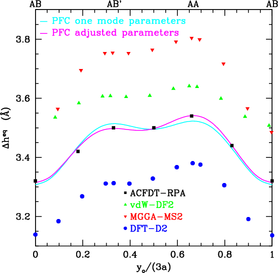
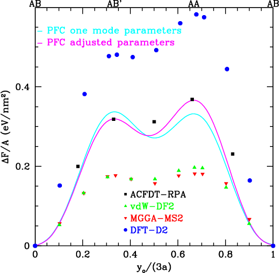
The free energy density difference (with area ) and the relative height were examined for the bilayer as a function of stacking position, where is the difference with respect to the AB stacking. The stacking is illustrated in Fig. 1, for densities and such that when an AB stacking (the lowest energy state) occurs. The parameters, as listed in Table 1, were initially chosen using the analytic one-mode approximation (which includes only the lowest-order Fourier coefficients needed to reconstruct the graphene and hBN crystalline lattices) as described by Elder et al. Elder et al. 2021. They were obtained by fitting to the DFT calculations of Zhou et al. Zhou et al. 2015 which considered four different DFT approaches and determined the one with the acronym ACFDT-RPA giving the best predictions for bulk properties; as such these data were used to fit the current PFC model. Their predictions for and equilibrium are shown in Figs. 2 and 3 respectively. Numerical simulations of the PFC model were conducted (which naturally include all Fourier coefficients) to minimize the free energy for an AB stacking. This configuration was then used to determine the energy of other stackings as described by Elder et al. Elder et al. 2021. As with the DFT calculations these were done on a single unit cell which does not allow for out-of-plane deformations. The outcomes of these studies show that results from the one-mode parameters are close to the DFT calculations but are slightly different with small deviations for the height and free energy density difference between the AB′ and AA stackings, as seen in Figs. 2 and 3. One particular feature is that in the one-mode predictions the magnitude of and are very similar for the AB′ and AA stackings which however are clearly different in all the DFT calculations. For this reason the parameters were adjusted to obtain a better fit as shown in both Figs. 2 and 3. A summary of the corresponding dimensionless parameters obtained are given in Table 1. These adjusted parameters are used in all the subsequent simulations that follow.
IV Inversion Domain Boundaries in hBN and the graphene/hBN bilayer
In a prior publication Taha et al. 2017 an examination of inversion boundaries in hBN was done using a rigid model, i.e., using the free energy functional in Eq. (6) with . An inversion boundary forms when the atomic ordering switches from BNBNBN to NBNBNB as illustrated in Fig. 4. As drawn in the figure the boundary contains many homoelemental nearest neighbours in the middle portion, which would be very unfavorable energetically. Instead the system prefers to form defected structures with unit rings that contain more or less than six atoms, but avoid having homoelemental BB or NN neighbouring. In particular, the grain boundary energy per unit length () of inversion boundaries that contain , , and defect structures will be studied, where corresponds to neighbouring defect pairs containing - and -membered atomic rings. In prior work Taha et al. 2017 it was found that the boundary naturally emerges when the boundary is along the armchair (AC) direction, while the results from the zigzag (ZZ) orientation. There was also a boundary along a ZZ interface that was slightly shifted; hence strictly speaking the is not an inversion boundary due to the shift (see Fig. 5).
In this section inversion boundaries will be examined for a flexible hBN monolayer and a hBN/graphene bilayer. These studies will illustrate the impact of allowing out-of-plane deformations on a single layer as well as the influence of the hBN inversion boundary on the graphene layer in a bilayer system.


Simulations were first conducted to reproduce the results of Taha et al. Taha et al. 2017. A fully periodic box of size , where and are integers, was used. In these simulations a box of grid size for the AC configuration and for the ZZ configuration were used. This corresponds to boxes of size Å Åfor the AC and Å Åfor ZZ, and corresponds to a single unit cell in the direction. It should be noted that conserved dynamics (i.e., Eq. (10)) were employed, which do not fix the local density while ensuring a constant average density in the whole system. Taha et al. Taha et al. 2017 typically found grain boundary energies saturate for system sizes of Å and larger. For the rigid case (without out-of-plane deformations) the initial condition was such that half the simulation box was of configuration NBNB while the other half was BNBN with a uniform density band of width placed at the boundaries. Simulations were run until the system energy was minimized. Next, and were varied to find the minimum energy state (since it is not possible to know the desired width of the domain walls). In the simulations here (flexible hBN monolayer and hBN/graphene bilayer) the same procedure was followed. Fixing reproduced the results of Taha et al. Taha et al. 2017 for the 2D rigid planar systems.
Following this simulations were conducted for a flexible sheet allowing out-of-plane deformations (i.e., containing variations in ). A first test was conducted on a system of size Å Å, with the initial condition set up by reproducing lattice constants for an AC boundary along the direction. The initial height was set to be a uniform random number in the range . The simulation results showed that the height developed into a one-dimensional pattern perpendicular to the domain wall (see Fig. 6(a)). This indicates that one unit cell along the parallel direction of this pattern was sufficient. Allowing for out-of-plane deformations lowered the domain wall energy, as shown in Fig. 5. Despite a modest bending of the sheet (of the order of one atomic spacing, as seen in, e.g., Fig. 6(a)), a considerable decrease of system energy was observed (by 8.0%, 13.9%, and 9.4% respectively for , , and boundaries).


A further simulation was conducted to understand the influence of such boundaries in g/hBN bilayers. The initial condition for the hBN layer was the same as that described for the monolayer case, except the lattice constant used ( Å) was the one that minimizes the g/hBN bilayer as discussed in Sec. III. The graphene layer was initialized to be in an AB stacking configuration on both sides of the grain boundary. Near the boundaries the graphene density was set to be uniform in a width of so that a boundary would naturally form. This leads to an inversion boundary in the hBN layer with defect pairs and a domain wall in the graphene layer, in which the graphene slides perpendicular to boundary, as illustrated in Fig. 7. As can be seen in this figure the graphene layer remains in the AB stacking but the atomic sites need to shift across the boundary, leading to in-plane local distortions and strain in the graphene layer. Initially the heights in both layers resemble that of the monolayer case; however as time evolves larger height gradients appeared at the boundaries, leading to numerical instabilities. In order to eliminate the instability the grid spacings in both the and the directions were reduced by a factor of two. With this change during the time evolution the heights spontaneously transformed into a much smoother profile eventually, as shown in Figs. 6(a) and 6(b).
The free energy difference per unit length was measured to be eV/Å for the inversion boundary in the g/hBN bilayer system. While it is somewhat interesting that this value is comparable to the single-layer result of hBN, it is important to note that in the single-layer system the inversion boundary energy was compared to an unstrained, flat equilibrium hBN layer (with lattice constant Å), while for the bilayer it was compared to a configuration with lattice constant Å that minimizes the bilayer, where both the graphene and hBN layers are strained in the lowest energy state. This significantly restricts out-of-plane deformations since the hBN layer is under compression and graphene under tension. In addition, the bilayer is a three-dimensional system. The three-dimensional inversion boundary energy, , is eV/Å2 = 0.142 eV/Å2, where Å is the vertical spacing between the layers.
While these simulations give insights of the influence of a defect (i.e., inversion boundary in hBN) in the coupled layers, it should be noted that the quantitative results will depend on the specific setup. In the above simulations an inversion boundary was formed in hBN at the equilibrium lattice constant (2.488 Å) of the g/hBN bilayer system. This would be quantitatively different from growing graphene on an already formed hBN inversion boundary that was at the lattice constant (2.51 Å) of a single hBN layer. In addition, the procedure in the simulations conducted here was to adjust the width and length of the system to minimize the free energy. Presumably changes in the setup and procedure could lead to quantitatively different results, although they are unlikely to change the qualitative structures in the two layers, such as the domain wall and its resulting strain in the graphene layer.

V Twisted Bilayers
To study a twisted bilayer of graphene and hBN numerically, one layer was rotated by an angle and the other by , for a total misorientation of , with both lattice constants set to those identified in Sec. III, i.e., 2.488Å. This gives rise to the appearance of Moiré patterns and some interesting behaviour as observed in many previous works Elder et al. 2021; Zhou et al. 2015; Elder et al. 2016; Elder et al. 2017. As discussed in Ref. Elder et al. 2021 only certain rotation angles and box sizes can be used in a periodic simulation box. More precisely, given an integer in the zigzag orientation with rotation angle
| (17) |
the system size must be
| (18) |
where . A typical configuration at a small angle is presented in Fig. 8. The wavelength, , of the Moiré pattern shown in this figure is given by . The figure indicates that the height difference is the smallest in the AB stacking regions and the largest at the AA junctions, followed by the AB′ junctions, consistent with Fig. 2. This makes the pattern slightly non-symmetric or tilted.

Sample configurations are shown in Fig. 9 for the corresponding free energy density and the volumetric stress, , of the whole system and individual layers. These quantities vary on the length scale of the atomic spacing, which makes it difficult to observe the overall pattern. For this reason in the visualization of patterns they were smoothed via the multiplication of in Fourier space, where is the wave number, and then an inverse Fourier transform. A value of was found to mostly eliminate the small scale oscillations while not washing out the large scale Moiré patterns, and was used for the pattern visualization of all angles. Figure 9 shows that the triple junctions in the pattern are slightly twisted, particularly evident in the spatial distribution of individual layers (see panels (c) and (d)), from which it is also interesting to note that the junctions in two layers twist in opposite directions. Similar twisted junctions have been observed in many other strained-layer Moiré patterns Elder et al. 2016; Tumino et al. 2015; Wu et al. 2011; Ling et al. 2006; Dai et al. 2016; Pushpa and Narasimhan 2003; Corso et al. 2010. This twisting occurs to move the junctions to lower the junction energy, even though this slightly increases the length of the domain walls connecting the junctions.


For very small angles it is possible to postulate that the system free energy would scale as , where is the free energy of the junction, is the energy per unit length of the domain wall, is the free energy density of the commensurate regions, and is the area of a hexagon in the pattern. The factor of in front of is due to the fact that each junction contributes to each hexagon and there are six junctions per hexagon. The factor in front of arises from the fact that each domain wall length is and that there are six domain walls per hexagon with each wall contributing to two hexagons. This then implies that the free energy density difference scales as
| (19) |
The total free energy density of the bilayer is shown as a function of the inverse periodicity () of the pattern in Fig. 10, which includes a fit to the form for the small angle data. This gives a prediction for the junction energy eV and domain wall energy density eV/nm. These results should be taken with a grain of salt as they assume is much larger than the size of the defects (domain walls and junctions) and that the specific form of defects does not change with system size. However, it is clear that there are in fact changes in these defects as shown in Fig. 11, where the free energy density across a domain wall can be seen to increase with larger system size.

The change in free energy density is also accompanied by a change in the buckling of the individual layers. In Fig. 12 the buckling width (where refers to the graphene (g) or hBN (h) layer) is depicted. The buckling reaches a maximum as and becomes very small for large angles as has been observed in other studies Kumar et al. 2015. Also shown in this figure is the average distance between the layers minus the equilibrium AB-stacking distance. As can be seen this distance is much smaller than the buckling of the individual layers, indicating that the sheets buckle in sync with each other as has been observed in graphene/graphene bilayers Zhou et al. 2015; Dai et al. 2016; Elder et al. 2021.


More interesting than the buckling is the change in stress as a function of misorientation. The picture of well-defined domain walls and junctions breaks down for large misorientations when the domain walls become comparable with the size of the Moiré pattern. This can be well captured by the volumetric () and von Mises Dantzig and Rappaz 2009 ( stresses, where the latter is given by in 2D after neglecting the -direction stress components. The corresponding results are shown in Fig. 13. The patterns exhibit a transition from those with well-defined triple junctions and domain walls to smeared-out patterns around (with nm). As can be seen in Fig. 11 the size of the domain wall is on the order of nm; thus the transition occurs roughly when the domain walls begin to overlap. In this case there are no well-defined AB, AB′ and AA regions as indicated in Fig. 14, which shows the occupancy of these states as a function of . It should be noted that it was not always possible to determine the state of a given unit cell; i.e., as shown in this figure the sum of the occupancy does not add to one. Clearly for small angles the AB states dominate since they are the lowest energy phases, followed by the next lowest energy state AB′ and finally by the AA state as expected. This also implies that for small angles the AA junctions are slightly smaller than the AB′ junctions.
The transition from small to large angle patterns can be identified from the average von Mises and volumetric stresses as given in Fig. 15. Both become larger with the increase of misorientation angle, then reach a peak before slowly decreasing. The peak in occurs at and in appears at , consistent with the observation in spatial profiles of stress distribution in Fig. 13 which show the transition between two different types of Moiré patterns. However, it is interesting to note the differences between the patterns. In the volumetric case the stress is largest in the commensurate regions and smallest at the domain walls. This is the exact opposite of the von Mises stress, which is most apparent at small misorientations, as seen in Fig. 13. The spatial difference between the two stresses is likely due to the fact that von Mises stress incorporates effects of distortion and shearing, and thus would be large at domain walls, while volumetric (hydrostatic) stress accounts for the effect of volume change but not distortion or shear, and thus would be small at domain boundaries but large in the domain bulk subjected to lattice compression or tension. In addition, in the volumetric case the stress increases in the commensurate regions with increasing angle until the transition to the smeared-out state occurs. In contrast, the von Mises stress in the commensurate regions does not vary as much with the change of misorientation. It appears that as the angle decreases from large values, domain walls emerge, which increases the von Mises stress until the walls are fully formed. When the angle is further reduced, the total von Mises stress decreases as the relative area of domain wall compared to well-separated commensurate region becomes smaller. This results in a maximum of average stress around a transition angle as shown in Fig. 15. This change of von Mises stress distribution indicates the change of mechanical property (e.g., yielding) of the bilayer across the transition of Moiré pattern.

As a final note it is interesting to contrast these results with the Moiré patterns that appear in graphene/graphene bilayers. The main difference is that in a graphene/graphene bilayer the AB′ stacking would have an energy identical to the AB stacking, i.e., in such a bilayer no AB′ junction would exist. This completely changes the symmetry of the domain wall and defect structures from triangular in graphene/graphene bilayers to honeycomb shape in g/hBN bilayers. A comparison of the two different systems is shown in Fig. 16 for two different misorientations. The commensurate regions (with lowest height differences, appearing yellow/light in the figure) of these two types of bilayers have inverse symmetry with respect to each other, i.e., a triangular pattern forms in the g/hBN bilayer and honeycomb in the graphene/graphene bilayer.
VI Summary and Conclusions
In this work a 2D PFC model incorporating out-of-plane deformations was examined for hBN and graphene/hBN bilayers. In the bilayer case, the model was parameterized numerically to closely match the ACFCT-RPA DFT calculations for stacking energies and height differences between the graphene and hBN layers obtained by Zhou et al. Zhou et al. 2015, which improves the previous analytic one-mode calculations of Ref. Elder et al. 2021. It was shown that out-of-plane deformations lead to significantly lower inversion boundary energies in hBN, on the order of %. The boundary in the g/hBN system results in the formation of a domain wall with local distortions in the graphene lattice. This interesting defect configuration in the g/hBN bilayer gives a domain wall energy of eV/Å2 as predicted from this PFC calculation.
Numerical simulations were conducted to examine the Moiré patterns that form when the bilayers are rotated with respect to each other, showing regions of different types of stacking positions between the layers. For small rotations the patterns consisted of well-defined hexagon-shaped domain walls with triple junctions twisting in opposite directions in graphene versus hBN layers. Results of the system free energy density, layer height difference, buckling, and smoothed volumetric and von Mises stresses have been obtained for a range of bilayer misorientation angles (and Moiré pattern wavelengths) that go beyond previous studies. An interesting phenomenon observed is the breakdown of well-distinguished domain wall structures in the Moiré pattern at large enough misorientation when the domain wall width and the pattern size are of compatible scale, leading to the transition to a different type of smeared-out Moiré pattern with overlapping domain boundaries. The corresponding elastic variations of these bilayer systems, in terms of volumetric and von Mises stresses, have been identified, serving as a useful way to characterize the Moiré pattern, transition, and the mechanical property of this type of vertical heterostructures.
Acknowledgements.
K.R.E. acknowledges support from the National Science Foundation (NSF) under Grant No. DMR-2006456 and Oakland University Technology Services high performance computing facility (Matilda). Z.-F.H. acknowledges support from NSF under Grant No. DMR-2006446. T.A-N. has been supported in part by the Academy of Finland through its QTF Center of Excellence program grant no. 312298. K.R.E. also acknowledges useful discussions with M. Greb.References
- Akinwande et al. (2019) D. Akinwande, C. Huyghebaert, C.-H. Wang, M. I. Serna, S. Goossens, L.-J. Li, H.-S. P. Wong, and F. H. L. Koppens, Nature 573, 507 (2019).
- Ajayan et al. (2016) P. Ajayan, P. Kim, and K. Banerjee, Phys. Today 69, 38 (2016).
- Guinea and Walet (2018) F. Guinea and N. R. Walet, Proc. Natl. Acad. Sci. USA 115, 13174 (2018).
- Yankowitz et al. (2019) M. Yankowitz, S. Chen, H. Polshyn, Y. Zhang, K. Watanabe, T. Taniguchi, D. Graf, A. F. Young, and C. R. Dean, Science 363, 1059 (2019).
- Momeni et al. (2020) F. Momeni, B. Mehrafrooz, A. Montazeri, and A. Rajabpour, Int. J. Heat Mass Transf. 150, 119282 (2020).
- Dean et al. (2013) C. R. Dean, L. Wang, P. Maher, C. Forsythe, F. Ghahari, Y. Gao, J. Katoch, M. Ishigami, P. Moon, M. Koshino, et al., Nature 497, 598 (2013).
- Hunt et al. (2013) B. Hunt, J. D. Sanchez-Yamagishi, A. F. Young, M. Yankowitz, B. J. LeRoy, K. Watanabe, T. Taniguchi, P. Moon, M. Koshino, P. Jarillo-Herrero, et al., Science 340, 1427 (2013).
- Moon and Koshino (2014) P. Moon and M. Koshino, Phys. Rev. B 90, 155406 (2014).
- Iwasaki et al. (2020) T. Iwasaki, S. Nakaharai, Y. Wakayama, K. Watanabe, T. Taniguchi, Y. Morita, and S. Moriyama, Nano Lett. 20, 2551 (2020).
- Tang et al. (2013) S. Tang, H. Wang, Y. Zhang, L. Ang, H. Xie, X. Liu, L. Liu, T. Li, F. Huang, X. Xie, et al., Sci. Rep. 3, 2666 (2013).
- Huang et al. (2021) X. Huang, L. Chen, S. Tang, C. Jiang, H. Wang, Z.-X. Shen, H. Wang, and Y.-T. Cui, Nano Lett. 21, 4292 (2021).
- Hu et al. (2017) C. Hu, V. Michaud-Rioux, X. Kong, and H. Guo, Phys. Rev. Materials 1, 061003 (2017).
- Chandra et al. (2020) Y. Chandra, E. I. Saavedra Flores, and S. Adhikari, Comp. Mat. Sci. 177, 109507 (2020).
- Hirvonen et al. (2016) P. Hirvonen, M. M. Ervasti, Z. Fan, M. Jalalvand, M. Seymour, S. Mehdi Vaez Allaei, N. Provatas, A. Harju, K. R. Elder, and T. Ala-Nissila, Phys. Rev. B 94, 035414 (2016).
- Taha et al. (2017) D. Taha, S. K. Mkhonta, K. R. Elder, and Z.-F. Huang, Phys. Rev. Lett. 118, 255501 (2017).
- Hirvonen et al. (2017) P. Hirvonen, Z. Fan, M. M. Ervasti, A. Harju, K. R. Elder, and T. Ala-Nissila, Sci. Rep. 7, 4754 (2017).
- Taha et al. (2019) D. Taha, S. R. Dlamini, S. K. Mkhonta, K. R. Elder, and Z.-F. Huang, Phys. Rev. Mater. 3, 095603 (2019).
- Waters and Huang (2022) B. Waters and Z.-F. Huang, Acta Mater. 225, 117583 (2022).
- Hirvonen et al. (2019) P. Hirvonen, V. Heinonen, H. Dong, Z. Fan, K. R. Elder, and T. Ala-Nissila, Phys. Rev. B 100, 165412 (2019).
- Huang (2022) Z.-F. Huang, Phys. Rev. Materials 6, 074001 (2022).
- Elder et al. (2021) K. R. Elder, C. V. Achim, V. Heinonen, E. Granato, S. C. Ying, and T. Ala-Nissila, Phys. Rev. Mater. 5, 034004 (2021).
- Zhou et al. (2015) S. Zhou, J. Han, S. Dai, J. Sun, and D. J. Srolovitz, Phys. Rev. B 92, 155438 (2015).
- Elder et al. (2007) K. R. Elder, N. Provatas, J. Berry, P. Stefanovic, and M. Grant, Phys. Rev. B 74, 064107 (2007).
- Guo et al. (2016) Y. Guo, J. Qui, and W. Guo, Nanotechnology 27, 505702 (2016).
- Elder et al. (2016) K. R. Elder, Z. Chen, K. L. M. Elder, P. Hivonen, S. K. Mkhonta, S.-C. Ying, E. Granato, Z.-F. Huang, and T. Ala-Nissila, J. Chem Phys. 144, 174703 (2016).
- Elder et al. (2017) K. R. Elder, C. V. Achim, E. Granato, S.-C. Ying, and T. Ala-Nissila, Phys. Rev. B 96, 195439 (2017).
- Tumino et al. (2015) F. Tumino, P. Carrozzo, L. Mascaretti, C. S. Casari, M. Passoni, S. Tosoni, C. E. Bottani, and A. L. Bassi, 2D Mater. 2, 045011 (2015).
- Wu et al. (2011) C. Wu, M. S. J. Marshall, and M. R. Castell, J. Phys. Chem. C 115, 8643 (2011).
- Ling et al. (2006) W. L. Ling, J. C. Hamilton, K. Thurmer, G. E. Thayer, J. de la Figuera, R. Q. Hwang, C. B. Carter, N. C. Bartelt, and K. F. McCarty, Surf. Sci. 600, 1735 (2006).
- Dai et al. (2016) S. Dai, Y. Xiang, and D. J. Srolovitz, Nano Lett. 16, 5923 (2016).
- Pushpa and Narasimhan (2003) R. Pushpa and S. Narasimhan, Phys. Rev. B 67, 205418 (2003).
- Corso et al. (2010) M. Corso, L. Fernández, F. Schiller, and J. E. Ortega, ACS Nano 4, 1603 (2010).
- Kumar et al. (2015) H. Kumar, D. Er, L. Dong, J. Li, and V. B. Shenoy, Sci. Rep. 5, 10872 (2015).
- Dantzig and Rappaz (2009) J. A. Dantzig and M. Rappaz, Solidification (EPFL Press, Lausanne, 2009).