KCL-PH-TH/2023-05

Cosmic bounce and phantom-like equation of state from tunnelling

Jean Alexandre Affiliation: Theoretical Particle Physics and Cosmology, King’s College London, WC2R 2LS, UK Email: jean.alexandre@kcl.ac.uk and Silvia Pla Affiliation: Theoretical Particle Physics and Cosmology, King’s College London, WC2R 2LS, UK Email: silvia.pla_garcia@kcl.ac.uk

Abstract

We allow a scalar field on a flat FLRW background metric to tunnel between two degenerate vacua. The resulting true vacuum state then violates the Null Energy Condition, and the corresponding homogeneous fluid induces a bounce, after which it has a phantom-like equation of state and asymptotically leads to a de Sitter phase. The mechanism presented here requires no exotic matter or modified gravity, it is purely generated by quantum fluctuations and is valid for a generic double well potential.

1 Introduction

Unlike spontaneous symmetry breaking (SSB), which occurs in infinite volume, tunnelling involves remarkable energetic features, among which a non-perturbative ground state with no classical analogue. This is at the origin of convexity of the effective potential for a scalar field Symanzik:1969ek; Coleman:1974jh; Iliopoulos:1974ur; Haymaker:1983xk; Fujimoto:1982tc; Bender:1983nc; Hindmarsh:1985nc; Plascencia:2015pga; Millington:2019nkw, and thus symmetry restoration.

The explicit calculation of the one-particle-irreducible (1PI) effective potential, taking into account several degenerate vacua, was done in Alexandre:2012ht; Alexandre:2022sho in the semi-classical approximation for the partition function. These studies assumed an $O(4)$ -symmetric Euclidean space-time, and the corresponding work at finite but low temperature was done in Alexandre:2022qxc and Alexandre:2023jsl. The latter works allow for the full tunnelling regime, involving a gas of Euclidean-time-dependent instantons relating two degenerate vacua. It was found that the true ground state for the scalar field is symmetric, and it violates the Null Energy Condition (NEC - see Rubakov:2014jja; Kontou:2020bta for reviews), because it is non-extensive in the thermodynamical sense. We note here that these results are independent of symmetry-restoration by the Kibble-Zurek mechanism Kibble:1976sj; Zurek:1985qw, which is valid at high temperatures and does not allow for the NEC to be violated.

The present work extends this tunnelling mechanism to a Friedmann-Lemaitre-Robertson-Walker (FLRW) background metric, where we study the backreaction of the fluid provided by the scalar true vacuum on the metric dynamics. Our assumptions do not involve exotic matter or modified gravity, but a finite volume and an adiabatic expansion instead, both to be defined in the next section. Our results arise purely from quantum fluctuations and they have no classical counterpart.

It is well known that in Quantum Field Theory (QFT) the energy conditions can be violated under certain circumstances. Some examples include the Casimir effect Casimir:1948, radiation from moving mirrors Davies:1977yv, or black hole evaporation Hawking:1975vcx. Another interesting example in curved backgrounds was obtained in Onemli:2002hr. The latter work studies a self-interacting massless field, therefore seeing only one vacuum, and not tunnelling. Also, the background is fixed as a de Sitter metric, whereas in our study the scale factor is determined by the backreaction of the scalar effective vacuum. Nevertheless, it is still possible for the stress-energy tensor to satisfy certain constraints, such as the Averaged Null Energy Condition (ANEC), which averages the NEC over timelike or null geodesics. The mechanism we propose here indeed does not violate the ANEC, since NEC violation is valid temporarily only - see Sec.4. We note that an eternal inflation scenario is described in Kontou:2020pdx, which also respects the ANEC.

In Sec.2 we describe the semi-classical approximation in which we evaluate the partition function, based on the different saddle points which are relevant for two degenerate vacua: two static configurations and a gas of instantons/anti-instantons. In the situation of non-degenerate vacua, the relevant configurations are the Coleman bounce Coleman1; Coleman2 and the shot Andreassen:2016cvx, with imaginary quantum fluctuations which arise from a negative eigenvalue in the fluctuation determinant Ai:2019fri. In the present case though, there are not any imaginary quantum corrections, since the (anti-) instantons are monotonic functions of Euclidean time Kleinert:2004ev.

The effective action is then derived in Sec.3 to the lowest order in the field, which is enough to confirm convexity and that the ground state is obtained for a vanishing field, unlike the situation of SSB. This calculation is done in the adiabatic approximation, assuming that the tunnelling rate is large compared to the space-time expansion rate. The vacuum energy induced by tunnelling violates the NEC, which results in a cosmic bounce if we start with a contracting universe. This is followed by an expansion with a phantom-like equation of state $w<-1$ , which asymptotically becomes de Sitter with $w=-1$ . The property $w<-1$ is usually related to a negative kinetic term in the potential (see Ludwick:2017tox for a review on phantom energy), but is not the case here: the vacuum we find is homogeneous and its energetic properties arise purely from quantum fluctuations, not from a specific bare action. We note that the origin of energies is not relevant to this mechanism, since the effective ground state energy is always lower than the degenerate bare energies, and it is this negative difference which induced NEC violation.

In Sec.4 we solve numerically the Friedmann equations, where we study the backreaction of the effective theory on gravity. As expected from NEC violation, the solution exhibits a cosmological bounce Steinhardt:2001st; Khoury:2001wf; Khoury:2001bz, known to provide an alternative to Cosmic Inflation Guth:1980zm; Linde:1981mu. The original idea to generate a bounce from a tunnelling-induced scalar field true vacuum was proposed in Alexandre:2019ygz; Alexandre:2021imu, in the context of an $O(4)$ -symmetric Euclidean space-time though, whereas we allow here for the full tunnelling regime, with finite volume and infinite Euclidean time.

Finally, the detailed calculations are presented in Appendix A, B and C.

2 Semi-classical approximation and saddle points

2.1 Assumptions

We consider the classical background metric

\text{d}s^{2}=-\text{d}t^{2}+a^{2}(t)\delta_{ij}\text{d}x^{i}\text{d}x^{j}~,

(1)

where the scale factor $a(t)$ is kept generic. The bare matter action is

S[\phi]=\int\text{d}^{4}x\sqrt{|g|}(L-j\phi)~,

(2)

where the Lagrangian $L$ involves a double-well potential, as well as a non-minimal coupling to the scalar curvature:

L=-\frac{1}{2}g^{\mu\nu}\partial_{\mu}\phi\partial_{\nu}\phi-\frac{1}{2}\xi R\phi^{2}-\frac{\lambda}{4!}(\phi^{2}-v^{2})^{2}-\bar{\Lambda}~.

(3)

For convenience, we have also added the cosmological constant term in the matter sector ( $\bar{\Lambda}=\kappa^{-1}\Lambda$ with $\kappa=8\pi G$ ) to account for vacuum energy effects after renormalisation. The important assumptions we make are the following:

•

Finite volume, which allows tunnelling between the degenerate vacua. We start from a fundamental flat spatial cell with volume $V_{0}$ and comoving volume $a^{3}(t)V_{0}$ , which can be thought of as a 3-torus, or a 3-sphere with large enough radius to neglect curvature. Although finite, we assume the parameters of the model to be such that quantisation of momentum can be ignored, and the periodic boundary conditions do not play a role. Related comments on the Casimir effect are given in Alexandre:2023jsl for tunnelling in flat space-time, and we focus here on the tunnelling features only;
•

Adiabatic approximation, where the expansion rate of the metric is assumed small compared to the tunnelling rate for matter. According to the discussion at the end of Sec.2.4, this is valid in the regime

$|H|\equiv\left|\frac{\dot{a}}{a}\right|\ll v\sqrt{\frac{\lambda}{\pi}}~\alpha^{3/2}~\exp(-\alpha^{3})~,$ (4)

where $\alpha^{3}(t)=a^{3}(t)S_{0}/\hbar$ and $S_{0}$ is the action for an instanton interpolating the two vacua $\pm v$ .

As a consequence of the second point, the scale factor $a(t)$ will be considered constant for the calculation of the matter effective theory, and its time dependence will be reinstated when we couple the matter effective theory to gravity.

2.2 Semi-classical approximation

We work here in Euclidean signature. In the semi-classical approximation, and focusing only on the matter sector for the reasons explained above, the partition function takes the form

Z[j]=\int{\cal D}[\phi]\exp(-S[\phi]/\hbar)\simeq\sum_{n}Z_{n}[j]~,

(5)

where

Z_{n}=F_{n}[j]\exp(-S[\phi_{n}]/\hbar)\equiv\exp(-\Sigma_{n}[j]/\hbar)~,

(6)

and $\phi_{n}$ are the different dominant contributions, the saddle points, which satisfy the equation of motion and minimise the action locally in the space of field configurations. $F_{n}[j]$ are the fluctuation factors for these saddle points, that we will calculate at one-loop, and $\Sigma_{n}[j]$ are the corresponding connected graphs generating functionals.

The saddle points $\phi_{n}$ satisfy then

-\frac{1}{\sqrt{g}}\frac{\delta S}{\delta\phi}=j~,

(7)

and since we consider two degenerate minima, a bubble-solution cannot form, since it would have an infinite radius Coleman1; Coleman2. Hence we focus on homogeneous saddle points only, which can depend on the Euclidean time tough. These saddle points obey

\ddot{\phi}+\frac{3\dot{a}}{a}\dot{\phi}-\xi R\phi+\frac{\lambda}{6}v^{2}\phi-\frac{\lambda}{6}\phi^{3}=j~,

(8)

where a dot represents a (Euclidean) time derivative. In the adiabatic approximation, the scale factor $a$ is assumed constant for the calculation of quantum fluctuations for matter, and we will therefore take $\dot{a}=0=R$ . We discuss below the static saddle points and the instanton gas, with their corresponding connected graphs generating functionals $\Sigma_{1}[j],\Sigma_{2}[j]$ and $\Sigma_{gas}[j]$ respectively.

Finally, we are interested in the tunnelling-induced effective potential, such that it is enough to consider a constant source $j$ . A spacetime-dependent source is necessary for the calculation of the derivative part of the effective action only.

2.3 Static saddle points

The static saddle points satisfy

v^{2}\phi-\phi^{3}=\frac{6j}{\lambda}~,

(9)

which, for $j<j_{c}\equiv\lambda v^{3}/(9\sqrt{3})$ , has two real solutions

\phi_{1}(j)=\frac{2v}{\sqrt{3}}\cos\left(\frac{\pi}{3}-\frac{1}{3}\arccos(j/j_{c})\right)~~~~\mbox{and}~~~~\phi_{2}(j)=-\phi_{1}(-j)~,

(10)

with the corresponding actions

	$\displaystyle S_{1}[j]$	$\displaystyle\equiv$	$\displaystyle S[\phi_{1}(j)]=\int\text{d}^{4}x\sqrt{g}\left(\bar{\Lambda}+v\,j-\frac{3}{2v^{2}\lambda}~j^{2}+\mathcal{O}(j^{3})\right)$		(11)
	$\displaystyle S_{2}[j]$	$\displaystyle\equiv$	$\displaystyle S[\phi_{2}(j)]=S_{1}[-j]~.$

The one-loop fluctuation factor for a static saddle point $\phi_{n}(j)$ is calculated in Appendix A, using the Schwinger proper time representation of the propagator. We find for the corresponding renormalised connected graphs generating functional

	$\displaystyle\Sigma_{n}[j]$	$\displaystyle=$	$\displaystyle\int\text{d}^{4}x\sqrt{g}\Bigg(\bar{\Lambda}_{R}+\frac{\lambda_{R}}{4!}(\phi_{n}^{2}-v_{R}^{2})$		(12)
			$\displaystyle\qquad\qquad+\frac{\hbar\lambda_{R}^{2}}{4608\pi^{2}}\Big(G(\phi_{n})+2(3\phi_{n}^{2}-v_{R}^{2})^{2}\ln\big((3\phi_{n}^{2}/v_{R}^{2}-1)/2\big)\Big)+j\phi_{n}\Bigg)$		(12)

with

G(\phi_{n})=-285v_{R}^{4}+366v_{R}^{2}\phi_{n}^{2}-81\phi_{n}^{4}\,,

(13)

and $\lambda_{R},v_{R},\bar{\Lambda}_{R}$ are the renormalised parameters given in Appendix A. The specific form (12), including the renormalised parameters, is chosen in such a way that, in the absence of source we have

\Sigma_{n}[0]=\int\text{d}^{4}x\sqrt{g}\,\bar{\Lambda}_{R}~,

(14)

which makes the discussion on vacuum energy simpler. Note that, in eq.(12), the static saddle points $\phi_{n}$ can be expressed as in eq.(10), where the parameters can be replaced by the renormalised ones, since they satisfy the equation of motion Alexandre:2022sho.

2.4 Instanton gas

We describe here Euclidean time-dependent saddle points. In the absence of a source, they obey the following equation

\ddot{\phi}+\omega^{2}\phi-\frac{\lambda}{6}\phi^{3}=0~,

(15)

where $\omega=v\sqrt{\lambda/6}$ , which corresponds to a problem of real-time classical mechanics in the upside-down potential

V(\phi)=-\frac{\lambda}{24}(\phi^{2}-v^{2})^{2}~,

(16)

represented in Fig. 1.

Refer to caption — Figure 1: The upside-down potential $V(\phi)$ in which the field oscillates. One instanton corresponds to the motion from infinitesimally close to one hilltop to infinitesimally close to the other.

The motion starting asymptotically close to a hilltop and ending asymptotically close to the other hilltop is given by the known solution

\phi_{inst}(j=0)=\pm v\tanh\left(\frac{\omega}{\sqrt{2}}(t-t_{1})\right)~,

(17)

where $t_{1}$ corresponds to the “jump", where the instanton goes through 0, and the corresponding action is

S[\phi_{inst}(j=0),\bar{\Lambda}=0]=a^{3}S_{0}~~~~\mbox{with}~~~~S_{0}\equiv\frac{4\sqrt{2}}{\lambda}\omega^{3}V_{0}~.

(18)

Indeed, the field spends a large (Euclidean) time close to a hilltop, with an exponentially small contribution to both the potential and the kinetic energy, and the main contribution to the action comes from the jump. For $p$ jumps, an exact saddle point is a series of periodic oscillations between the two hills. If the motion starts exponentially close to a hilltop, the distance $|t_{i+1}-t_{i}|$ between two consecutive jumps is large compared to the width $2\pi/\omega$ of a jump. The motion is then approximately described by

\phi_{inst}^{(p)}(j=0)\simeq~\pm v\tanh\left(\frac{\omega}{\sqrt{2}}(t-t_{1})\right)\times\tanh\left(\frac{\omega}{\sqrt{2}}(t-t_{2})\right)\times\cdots\times\tanh\left(\frac{\omega}{\sqrt{2}}(t-t_{p})\right)~,

(19)

where the times $t_{i}$ are regularly spread along the Euclidean time (see Fig.2(a)), and the corresponding action is

S[\phi_{inst}^{(p)}(j=0),\bar{\Lambda}=0]\simeq p~a^{3}S_{0}~.

(20)

The above action remains unchanged when the jumps are shifted though, provided the condition $|t_{i+1}-t_{i}|\gg 2\pi/\omega$ is satisfied, which is called the dilute gas approximation (see Fig.2(b)). As a consequence, all the corresponding configurations in the path integral $Z$ contribute as much as the exact solution of the equation of motion. The invariance of the action under the translation of jumps has a high degeneracy, making this dilute gas dominant in $Z$ .

We show in Appendix B that, in the presence of a source, the summation over all the $p$ -jump saddle points leads to

\Sigma_{gas}[j]\simeq\frac{1}{2}\big(\Sigma_{1}[j]+\Sigma_{2}[j]\big)-\hbar\ln\big(\exp(\bar{N})-1\big)\equiv-\hbar\ln Z_{gas}[j]~,

(21)

where the statistical average number of jumps between the two static saddle points is

\bar{N}=\sqrt{g_{00}}~\omega T\sqrt{\frac{6a^{3}S_{0}}{\hbar\pi}}e^{-a^{3}S_{0}/\hbar}~.

(22)

We note that the parameters in the latter equation can be understood as the renormalised ones, since the contribution of $\bar{N}$ is at one-loop already.

The exponential of $\bar{N}$ appearing in the partition function is a known feature in tunnelling studies, and it arises from the summation over the zero modes of each (anti-) instanton (see Appendix B for details). Note that we are interested here in the situation where $S_{0}$ is fixed and the total Euclidean time $T$ goes to infinity, such that $\bar{N}$ is assumed to be large. An alternative situation, relevant at finite temperature, consists in fixing $T$ and taking $S_{0}\to\infty$ , such that $\bar{N}\to 0$ . This corresponds to the suppression of tunnelling, and where SSB provides a better description of the system Alexandre:2022qxc. The expression (22) can be understood as the total Euclidean time $T$ multiplied by the tunnelling rate $\omega\sqrt{6a^{3}S_{0}/\hbar\pi}~e^{-a^{3}S_{0}/\hbar}$ .

3 Effective action

We describe here the main steps for the construction of the effective theory, as well as its energetic properties. The details can be found in Appendix (C).

3.1 Symmetric ground state

From the previous section, the partition function can be expressed as

	$\displaystyle Z[j]$	$\displaystyle\simeq$	$\displaystyle Z_{1}[j]+Z_{2}[j]+Z_{gas}[j]$		(23)
		$\displaystyle=$	$\displaystyle\exp\left(-\frac{1}{\hbar}\Sigma_{1}[j]\right)+\exp\left(-\frac{1}{\hbar}\Sigma_{2}[j]\right)+(\exp(\bar{N})-1)\exp\left(-\frac{1}{2\hbar}\Big(\Sigma_{2}[j]+\Sigma_{2}[j]\Big)\right)~,$		(23)

from which one can derive the classical field $\phi_{c}$ , which corresponds to the vacuum expectation value in the presence of the source $j$

\phi_{c}=\frac{-\hbar}{Z(j)\sqrt{g}}\frac{\delta Z}{\delta j}=-M^{-2}\,j+{\cal O}(j^{3})~.

(24)

In the previous expression and in the limit where $T\to\infty$ , we show in Appendix C that

M^{-2}=\frac{3}{\lambda_{R}v_{R}^{2}}\left(1+\frac{27\hbar\lambda_{R}}{32\pi^{2}}\right)+\mathcal{O}(\hbar^{2})~.

(25)

We note that $\phi_{c}$ is proportional to $j$ , showing symmetry restoration: the vacuum for $j=0$ is at $\phi_{c}=0$ .
The relation $\phi_{c}[j]$ is then inverted to

j[\phi_{c}]=-M^{2}\phi_{c}+{\cal O}(\phi_{c}^{3})~,

(26)

and the 1PI effective action, defined through the Legendre transform as a functional of $\phi_{c}$ , is

	$\displaystyle\Gamma[\phi_{c}]$	$\displaystyle=$	$\displaystyle-\hbar\ln Z[j\big[\phi_{c}]\big]-\int\text{d}^{4}x\sqrt{g}~\phi_{c}~j[\phi_{c}]$		(27)
		$\displaystyle=$	$\displaystyle\Gamma[0]+\frac{1}{2}\int\text{d}^{4}x\sqrt{g}~M^{2}\phi_{c}^{2}+\mathcal{O}(\phi_{c}^{4})~.$		(27)

In the previous expression, the effective action for the ground state reads

	$\displaystyle\Gamma[0]$	$\displaystyle=$	$\displaystyle\int\text{d}^{4}x\sqrt{g}\,\bar{\Lambda}_{R}-\hbar\ln(e^{\bar{N}}+1)$		(28)
		$\displaystyle\simeq$	$\displaystyle\int\text{d}^{4}x\sqrt{g}\,\bar{\Lambda}_{R}-\hbar\bar{N}~.$		(28)

To summarise the essential features of the effective action (27):

•

it is convex, since $M^{2}>0$ , and has its ground state at $\phi_{c}=0$ ;
•

the ground state energy has a non-trivial dependence on the comoving volume, via $\bar{N}$ , and is therefore not extensive in the usual thermodynamical sense.

3.2 NEC violation

For simplicity, in what follows we will drop the sub-index _R and all the parameters should be understood as the renormalised ones.

We focus here on the fluid provided by the ground state $\phi_{c}=0$ . In order to obtain the energy density and the pressure, we need to represent $\Gamma[0]$ and thus $\bar{N}$ as the integral over a Lagrangian density, restoring the time dependence of the scale factor. This is done in Appendix C, where we show that the expression (28) can be written as

\displaystyle\Gamma[0]=\int\text{d}^{4}x\sqrt{g}\left(\bar{\Lambda}-\rho_{0}~\frac{e^{-\alpha^{3}}}{\alpha^{3/2}}\right)~,

(29)

where

\alpha^{3}\equiv a^{3}\frac{S_{0}}{\hbar}~~~~\mbox{and}~~~~\rho_{0}\equiv\hbar\,\frac{\omega}{V_{0}}\frac{S_{0}}{\hbar}\sqrt{\frac{6}{\pi}}=\frac{2\,\lambda~v^{4}}{3\sqrt{3\pi}}~.

(30)

From eq.(29), the energy density and the pressure are obtained from the components of the energy-momentum tensor

T_{\mu\nu}=\frac{2}{\sqrt{g}}\frac{\delta\Gamma[0]}{\delta g^{\mu\nu}}~,

(31)

and we find

	$\displaystyle\rho$	$\displaystyle=$	$\displaystyle\bar{\Lambda}-\rho_{0}~\frac{e^{-\alpha^{3}}}{\alpha^{3/2}}~,$		(32)
	$\displaystyle p$	$\displaystyle=$	$\displaystyle-\bar{\Lambda}+\rho_{0}\left(\frac{1}{2\alpha^{3/2}}-\alpha^{3/2}\right)e^{-\alpha^{3}}~.$

The fluid provided by the ground state therefore features the following properties:

•

It consistently satisfies the (real-time) continuity equation $\dot{\rho}+3H(\rho+p)=0$ ;
•

It violates the NEC

$\rho+p=-\rho_{0}~e^{-\alpha^{3}}\left(\alpha^{3/2}+\frac{1}{2\alpha^{3/2}}\right)~<0~;$ (33)
•

It can induce a cosmic bounce since it can simultaneously satisfy $\rho=0$ and $\rho+3p<0$ . Assuming $\bar{\Lambda}>0$ , the second condition is automatically satisfied if the NEC is violated;
•

Assuming $e^{-\alpha^{3}}\ll 1$ , its equation of state has the phantom form

$w=\frac{p}{\rho}\simeq-1-\frac{\rho_{0}}{\bar{\Lambda}}\,e^{-\alpha^{3}}\left(\alpha^{3/2}+\frac{1}{2\alpha^{3/2}}\right)~<-1~.$ (34)

We stress here an important point: the property $w<-1$ does not arise from a kinetic energy with the opposite sign, but is a consequence of tunnelling between the two degenerate bare vacua, which induces a homogeneous symmetric ground state.

4 Friedmann Equations

In this section we go back to Lorentzian signature. As explained in the introduction, we study the back-reaction of the effective theory on the metric, such that the energy-momentum tensor in the Einstein equations $G_{\mu\nu}=\kappa T_{\mu\nu}$ contains the energy density and pressure given by eqs. (32), and $\kappa$ is the renormalised gravity coupling. The resulting Friedmann equations read

	$\displaystyle H^{2}$	$\displaystyle=$	$\displaystyle\frac{\kappa}{3}\rho$		(35)
	$\displaystyle\frac{\ddot{a}}{a}$	$\displaystyle=$	$\displaystyle-\frac{\kappa}{6}(\rho+3p)~,$

that we study here numerically. The first equation $H^{2}\propto\rho$ gives the initial condition $\dot{a}_{0}$ once $a_{0}$ is known, and the second equation provides the evolution equation for $a(t)$ . We then introduce the dimensionless time

\tau\equiv t~\sqrt{\frac{\Lambda}{3}}~,

(36)

and we use the expressions (32) to obtain from eqs.(35)

	$\displaystyle\alpha^{\prime}$	$\displaystyle=$	$\displaystyle\pm\alpha\sqrt{1-r~\frac{e^{-\alpha^{3}}}{\alpha^{3/2}}}$		(37)
	$\displaystyle\frac{\alpha^{\prime\prime}}{\alpha}$	$\displaystyle=$	$\displaystyle 1-\frac{r~e^{-\alpha^{3}}}{4~\alpha^{3/2}}(1-6\alpha^{3})~,$

where a prime denotes a derivative with respect to $\tau$ and

r=\kappa\frac{\rho_{0}}{\Lambda}=\frac{\rho_{0}}{\bar{\Lambda}}~.

(38)

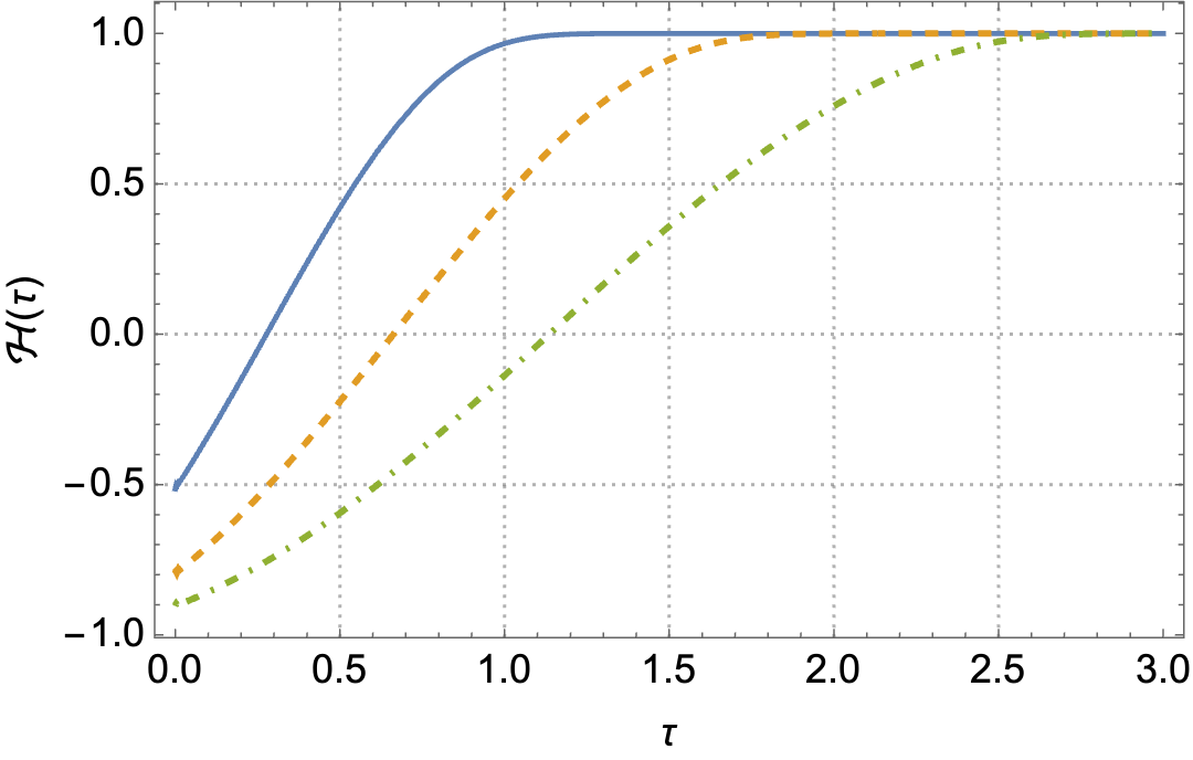
The Friedmann Equations (37) are solved numerically, and we plot in Figure 3 the solutions corresponding to a fixed value of $\alpha(0)$ and different values of the parameter $r$ . The initial condition for $\alpha^{\prime}(0)$ is given by the negative branch $\alpha^{\prime}(0)<0$ of the first Friedmann equation, in order to describe a cosmological bounce, which will occur if $\rho=0$ and $\rho+3p<0$ are simultaneously satisfied at a given time $t_{b}$ . We see that such a bounce is indeed generated, after which the expansion suppresses tunnelling: the NEC is recovered and the metric dynamics enters a de Sitter phase, with constant $H$ .

5 Conclusions

We have described how the energetic properties arising from tunnelling could be relevant in a cosmological context, starting from standard QFT and Einstein gravity. To summarise the non-perturbative mechanism described in this article:

1.

The effective theory taking into account tunnelling between two degenerate vacua is obtained by considering the contribution of different saddle points in the partition function;
2.

As a consequence of this interplay between the two vacua $\pm v$ , the resulting true vacuum is at $\phi_{c}=0$ , with an energy which is not proportional to the comoving volume;
3.

This non-extensive feature of the vacuum energy implies NEC violation;
4.

The NEC violation induces a cosmological bounce in the case of initial spacetime contraction, and is valid until the resulting expansion suppresses tunnelling, such the ANEC is satisfied.

The adiabatic approximation is well justified in the vicinity of the cosmological bounce, but out-of-equilibrium studies would be necessary to include the full-time dependence of the scale factor if one wishes to look at what happens away from the bounce. A related improvement to this work would be to derive our results in a manifestly covariant way.

Regarding the assumption of finite-volume FLRW space-time, this study has required a toy-model geometry/topology, in the form of a 3-torus or 3-sphere, and thus still needs to be developed for phenomenological purposes. Also, quantum corrections in a finite volume should in principle take into account discrete momentum, as well as periodic boundary conditions. This is done in the framework of Casimir effect studies Bordag:2001qi, whereas the present article focuses on the tunnel effect, with continuous momentum and effectively Dirichlet boundary conditions. A natural step further would then consider a discrete spectrum, which could be done numerically for example.

The situation of non-degenerate minima would avoid making the finite-volume assumption, since the relevant instanton action (the Coleman bounce saddle point) is independent of the volume. In this case, quantum fluctuations for the latter saddle point would involve an imaginary part, which should be cancelled by the imaginary part induced by other saddle points Andreassen:2016cvx, since the effective potential is real. The whole process is challenging to describe analytically in more than 0-dimensional space-time though, but is a potential avenue to explore, since it could be relevant as a component of Dark Energy (see related comment below). There are questions which remain to be answered in the situation of non-degenerate minima though, one of which is the possibility to obtain a NEC-violating effective ground state. Indeed, if one considers only $O(4)$ -symmetric saddle points, the NEC should not be violated since space and (Euclidean) time are treated in the same way. A more complex saddle point structure, to be studied in the context of real-time tunnelling Ai:2019fri, could involve NEC violation though, but this study goes beyond the scope of the present article. Another question in this context is the use of a homogeneous classical field, which would be valid at large scales only (large compared to the radius of a 4-dimensional bubble), in order to describe an average over the gas of bubbles. But strictly speaking, the homogenous configurations used in the present work are valid for a second-order quantum phase transition only, whereas the presence of bubbles is a signature for a first order phase transition.

In our model, the universe asymptotically approaches a de Sitter phase in the late-time regime, from which one cannot escape. This phase could potentially represent Dark Energy in the late Universe, where we would need to identify $\Lambda$ with the current cosmological constant. Given our numerical study where $r\sim 1$ , and assuming $S_{0}\sim\hbar$ for tunnelling to be significant, we find from the expressions (18), (30) and (38) for $S_{0}$ , $\rho_{0}$ and $r$ respectively, that

\Lambda\sim\hbar\sqrt{\frac{\lambda}{\pi}}\frac{\kappa v}{V_{0}}~.

(39)

The latter order of magnitude allows an estimate of the volume $V_{0}$ at the bounce, which should be much smaller than the volume $V$ of the current visible Universe, for tunnelling to be significant enough. $V_{0}$ should also be much larger than the Plank volume $V_{P}$ , for the classical gravity regime to be valid. We obtain then the constraint

V_{P}\ll\hbar\sqrt{\frac{\lambda}{\pi}}~\frac{\kappa v}{\Lambda}\ll V~,

(40)

which could be helpful in model building for a bouncing Cosmology scenario. In any case, one should be careful when drawing conclusions far from the bounce, since our approach is based on equilibrium QFT, which is valid only in the vicinity of the bounce, i.e. when the condition (4) is satisfied. A more complete study would involve the Keldysh formalism for example, allowing out-of-equilibrium predictions, and which is a potential next step.

Acknowledgements

The authors thank Katy Clough and Malcolm Fairbairn for cosmology-related discussions, as well as Jose Navarro-Salas and Janos Polonyi for insightful comments. This work is supported by the Leverhulme Trust (grant RPG-2021-299) and the Science and Technology Facilities Council (grant STFC-ST/T000759/1). For the purpose of Open Access, the authors have applied a CC BY public copyright licence to any Author Accepted Manuscript version arising from this submission.

Appendix A One-loop effective action in curved space-times

In this appendix we review the main steps to obtain the one-loop effective action in curved space-times for a real scalar field in a double-well potential, and propagating in a curved background with Euclidean signature. We focus here on one saddle point only.

For renormalisation purposes, we need to consider the bare action of this model

S[\phi,g]=\int\text{d}^{d}x\sqrt{g}\left(\frac{1}{2}g^{\mu\nu}\partial_{\mu}\phi\partial_{\nu}\phi+\frac{1}{2}\xi R\phi^{2}+\frac{\lambda}{4!}(\phi^{2}-v^{2})^{2}+\bar{\Lambda}+j\phi\right)~,

(41)

together with the semi-classical action for gravity¹¹ 1 We note that the Euclidean form of the Lagrangian differs with a minus sign with respect to its Lorentzian form.

S_{G}[g]=-\int\text{d}^{d}x\sqrt{g}\Big[(2\kappa)^{-1}R+(\epsilon_{1}R^{2}+\epsilon_{2}R^{\mu\nu}R_{\mu\nu}+\epsilon_{3}R^{\mu\nu\rho\sigma}R_{\mu\nu\rho\sigma})\Big]~,

(42)

in $d$ space-time dimensions, where $\kappa=8\pi G$ , and $\bar{\Lambda}=\kappa^{-1}\Lambda$ . For convenience, we have included the cosmological constant term in the matter sector. The inclusion of the higher curvature terms is needed for the cancellation of the divergences that arise in this context. In this setup, the Klein-Gordon equation for the scalar field is

(-\Box_{E}+\xi R-\tfrac{\lambda}{6}v^{2}+\tfrac{\lambda}{3!}\phi^{2})\phi+j=0~,

(43)

where $\Box_{E}=g^{\mu\nu}\nabla_{\mu}\nabla_{\nu}=\frac{1}{\sqrt{g}}\partial_{\mu}(\sqrt{g}g^{\mu\nu}\partial_{\mu})$ , and the scalar field can be expanded around a saddle point $\phi=\phi_{s}+\delta\phi$ . The associated Euclidean Green’s function for the quantum fluctuation $\delta\phi$ reads

(-\Box_{E}+Q)G_{E}(x,x^{\prime})=\frac{1}{\sqrt{g}}\delta^{(4)}(x-x^{\prime})\,,

(44)

where

Q=\frac{\lambda}{2}\phi_{s}^{2}-\frac{\lambda v^{2}}{6}+\xi R\,.

(45)

The one-loop correction to the classical action can be written in terms of the Green’s function as parker-toms

	$\displaystyle\Sigma[\phi_{s},g]$	$\displaystyle=$	$\displaystyle S_{G}[g]+S[\phi_{s},g]-\tfrac{1}{2}\hbar\,\textrm{ln}\,\textrm{Det}\,G_{E}\,$		(46)
		$\displaystyle\equiv$	$\displaystyle S_{G}[g]+S[\phi_{s},g]+\Sigma^{(1)}[\phi_{s},g]\,.$		(46)

For general background configurations, the Green’s function is unknown. However, an approximated expression for the quantum contribution $\Sigma^{(1)}[\phi_{s},g]$ in the case of slowly varying background fields $\phi_{s}$ and $g$ can be computed using the proper-time formalism as follows (see Refs. Hu-lambdaphi4; Rajantie18 for a detailed explanation).

The DeWitt-Schwinger representation of the propagator $G_{E}(x,x^{\prime})$ is given by

G_{E}(x,x^{\prime})=\int_{0}^{\infty}\text{d}s\,H(x,x^{\prime};s)\,,

(47)

where the kernel $H(x,x^{\prime};s)$ obeys a diffusion equation with appropriate boundary conditions Vassilevich03. For the one-loop connected graph, it translates into

\Sigma^{(1)}[\phi_{s},g]=\,\frac{\hbar}{2}\int\text{d}^{d}x\sqrt{g}\int_{0}^{\infty}\frac{\text{d}s}{s}\,H(x,x;s)\,.

(48)

The kernel $H(x,x^{\prime};s)$ admits, in general, an asymptotic expansion in terms of the Schwinger proper-time parameter Schwinger51. At coincidence $x^{\prime}\to x$ this expansion reads

H(x,x;s)=\frac{e^{-m^{2}s}}{(4\pi s)^{d/2}}\sum_{k=0}^{\infty}a_{k}(x)\,s^{k}\,.

(49)

where $a_{k}(x)$ are the so-called the deWitt coefficients and $d$ is the space-time dimension. The first few coefficients are Gilkey75; Vassilevich03

$\displaystyle a_{0}$	$\displaystyle=$	$\displaystyle 1\,;$	(50)
$\displaystyle a_{1}$	$\displaystyle=$	$\displaystyle\frac{1}{6}R-Q\,;$	(51)
$\displaystyle a_{2}$	$\displaystyle=$	$\displaystyle-\frac{1}{180}R_{\alpha\beta\gamma\delta}R^{\alpha\beta\gamma\delta}-\frac{1}{180}R^{\alpha\beta}R_{\alpha\beta}-\frac{1}{30}\Box_{E}R$	(52)
		$\displaystyle+\frac{1}{6}\Box_{E}Q+\frac{1}{2}Q^{2}-\frac{1}{6}RQ+\frac{1}{72}R^{2}\,.$	(52)

This expansion captures, in its leading orders, the UV divergences ( $s\to 0$ ) of the theory and it is routinely used for renormalisation in the context of QFT in curved spaces.

The expansion above (49) has an important property: it admits an exact resummation R-summed1; R-summed2

H(x,x;s)=\frac{e^{-\mathcal{M}^{2}s}}{(4\pi s)^{d/2}}\sum_{k=0}^{\infty}b_{k}(x)\,s^{k}\,,

(53)

with

\mathcal{M}^{2}=Q-\frac{1}{6}R\,,

(54)

such that, the new coefficients $b_{k}(x)$ do not contain any term that vanish when $Q$ and $R$ are replaced by zero. For example, for the first resummed deWitt coefficients we have

$\displaystyle b_{0}$	$\displaystyle=$	$\displaystyle 1\,;$	(55)
$\displaystyle b_{1}$	$\displaystyle=$	$\displaystyle 0\,;$	(56)
$\displaystyle b_{2}$	$\displaystyle=$	$\displaystyle-\frac{1}{180}R_{\alpha\beta\gamma\delta}R^{\alpha\beta\gamma\delta}-\frac{1}{180}R^{\alpha\beta}R_{\alpha\beta}-\frac{1}{30}\Box_{E}R+\frac{1}{6}\Box_{E}Q~.$	(57)

Therefore, the resummed expansion becomes a derivative expansion in the field $\phi_{s}$ and the metric, physically meaningful in the case of slowly varying background fields. Then, it is possible to truncate the expansion at a given order $N$ - the order of derivatives - to obtain an approximated expression for the one-loop connected graph

\Sigma^{(1)}[\phi_{s},g]=\,\frac{\hbar}{2}\int\text{d}^{d}x\sqrt{g}\int_{0}^{\infty}\frac{\text{d}s}{s}~~\frac{e^{-\mathcal{M}^{2}s}}{(4\pi s)^{d/2}}\sum_{k=0}^{N}b_{k}(x)\,s^{k}\,.

(58)

The expression above is divergent for $d=4$ and can be renormalised using dimensional regularization. For arbitrary dimension $d$ , the proper-time integrals can be performed to give

\Sigma^{(1)}[\phi_{s},g]=\frac{\hbar}{(4\pi)^{d/2}}\left(\frac{\mathcal{M}}{\mu_{d}}\right)^{d-4}\int\text{d}^{d}x\sqrt{g}~\sum_{k=0}^{N}b_{k}(x)\mathcal{M}^{d-2k}\,\Gamma\left(k-\frac{d}{2}\right)~.

(59)

We have introduced a renormalisation mass parameter to proceed with dimensional regularization in what follows. Truncating the sum at $N=2$ and expanding around $d\to 4$ we find

\Sigma^{(1)}=\hbar\int\text{d}^{4}x\sqrt{g}\left[\frac{\mathcal{M}^{4}}{64\pi^{2}}\Big[\ln\left(\frac{\mathcal{M}^{2}}{\mu^{2}}\right)-\frac{3}{2}\Big]+\frac{b_{2}}{32\pi^{2}}\ln\left(\frac{\mathcal{M}^{2}}{\mu^{2}}\right)\right]~,

(60)

where $\mathcal{M}^{2}>0$ since we quantise about stable saddle points and the curvature effects are expected to be small. In the above expression, the divergences have been absorbed in the scale parameter $\mu$ , which is defined by

\ln\mu^{2}=\ln\Big(4\pi\mu_{d}^{2}\Big)-\gamma-\frac{2}{d-4}~~~(\mbox{finite when}~d\to 4)~.

(61)

From these expressions, we can directly obtain the renormalised values of the coupling constants of the problem (see, for example Ref. Hu-book).

In our particular problem, we are assuming an adiabatic expansion of the universe, and that quantum processes under consideration occur at equilibrium. Hence, we neglect the curvature of space-time. Hence we are only interested in the couplings $\lambda,~v,~\bar{\Lambda}$ . For simplicity, we will follow Markkanen13, and apply the renormalisation conditions at the same scale for all bare parameters, namely,

\displaystyle 3\frac{\partial^{2}L}{\partial\phi^{2}}\Big|_{\phi=\pm v_{R},g=\eta}=\lambda_{R}\,v_{R}^{2}\,,\qquad\frac{\partial^{2}L}{\partial\phi^{4}}\Big|_{\phi=\pm v_{R},g=\eta}=\lambda_{R}\,,\qquad+L\Big|_{\phi=\pm v_{R},g=\eta}=\bar{\Lambda}_{R}~,

(62)

where $\eta$ is the Euclidean flat metric and $\Sigma=\int\text{d}^{4}x\sqrt{g}~L$ . From these conditions we obtain

$\displaystyle\delta\lambda$	$\displaystyle=$	$\displaystyle\frac{3\lambda_{R}^{2}}{32\pi^{2}}\left(3+\ln(\frac{v_{R}^{2}\lambda_{R}}{3\mu^{2}})\right)\,,$	(63)
$\displaystyle\delta v^{2}$	$\displaystyle=$	$\displaystyle\frac{v_{R}^{2}\lambda_{R}}{16\pi^{2}}\left(10-\ln(\frac{v_{R}^{2}\lambda_{R}}{3\mu^{2}})\right)\,,$	(64)
$\displaystyle\delta\bar{\Lambda}$	$\displaystyle=$	$\displaystyle\frac{v_{R}^{4}\lambda_{R}^{2}}{1152\pi^{2}}\left(-3+2\ln(\frac{v_{R}^{2}\lambda_{R}}{3\mu^{2}})\right)~,$	(65)

where we define $\lambda_{R}=\lambda+\hbar~\delta\lambda$ , $v_{R}^{2}=v^{2}+\hbar~\delta v^{2}$ , and $\bar{\Lambda}_{R}=\bar{\Lambda}+\hbar~\delta\bar{\Lambda}$ . Inserting these results in (46) and assuming $R=0$ and $\phi_{s}$ static, we obtain the final renormalised connected graph given in Sec. 2.3.

For completeness, we also give the renormalised values of $\kappa^{-1}$ and $\xi$ . The renormalisation conditons we impose are

-2\frac{\partial L}{\partial R}-\xi_{R}\phi^{2}\Big|_{\phi=\pm v_{R},g=\eta}=\kappa^{-1}_{R}\,,\qquad\frac{\partial^{3}L}{\partial R\partial\phi^{2}}\Big|_{\phi=\pm v_{R},g=\eta}=\xi_{R}\,,

(66)

that lead to

	$\displaystyle\delta\xi$	$\displaystyle=$	$\displaystyle\frac{\lambda_{R}(6\xi_{R}-1)}{192\pi^{2}}\left(3+\ln(\frac{v_{R}^{2}\lambda_{R}}{3\mu^{2}})\right)\,,$		(67)
	$\displaystyle\delta(\kappa^{-1})$	$\displaystyle=$	$\displaystyle\frac{v_{R}^{2}\lambda_{R}(6\xi_{R}-1)}{2304\pi^{2}}\left(11+\ln(\frac{v_{R}^{2}\lambda_{R}}{3\mu^{2}})\right)\,.$		(68)

Appendix B Quantisation over instanton configurations

In Section 2.4 we describe few features of the gas of instantons for a vanishing source. In the presence of an infinitesimal source $j\ll j_{c}$ , the jump is not modified, and what changes is the position of the asymptotically "flat" parts of the instantons, which now go from one saddle point $\phi_{i}(j)$ to the other, instead of going from one vacumm $\pm v$ to the other $\mp v$ . We have then, instead of eq.(18),

S[\phi_{inst}(j)]\simeq a^{3}S_{0}+\frac{1}{2}\big(S_{1}[j]+S_{2}[j]\big)~,

(69)

since on average the configuration spends half the Euclidean time exponentially close to $\phi_{1}(j)$ and the other half close to $\phi_{2}(j)$ . The contribution of one instanton $F_{inst}\exp(-S[\phi_{inst}]/\hbar)$ to the partition function is the product of the following contributions

•

The "flat" part close to each static saddle point, leading to the fluctuation factor $F_{i}$ about each of the static saddle points, for half of the total Euclidean time

$\sqrt{F_{1}F_{2}}e^{-(S_{1}+S_{2})/(2\hbar)}=\exp\left(-\frac{1}{2\hbar}\big(\Sigma_{1}[j]+\Sigma_{2}[j]\big)\right)~,$ (70)

where $\Sigma_{n}[j]$ is given in eq.(12).
•

Fluctuations above one jump which, discounting the zero mode corresponding to the translational invariance of the jump, lead to the factor (see Kleinert:2004ev; Dunne2009)

$\sqrt{\frac{6a^{3}S_{0}}{\hbar\pi}}~;$ (71)
•

The zero mode corresponding to the position of the jump, which can happen at any Euclidean time between 0 and $T$ , and thus gives the extra factor

$\omega\int_{0}^{T}\sqrt{g_{00}}~\text{d}t=\sqrt{g_{00}}~\omega T~.$ (72)

Note that the summation over the different positions of the jump is done with the comoving proper time, since the jump is observed by the comoving observer. Here, $S_{0}$ and $\omega$ are defined with the renormalised parameters.

All together, the contribution of one instanton to the partition function is

F_{inst}\exp\left(-\frac{S[\phi_{inst}]}{\hbar}\right)=\sqrt{g_{00}}~\omega T\sqrt{\frac{6a^{3}S_{0}}{\hbar\pi}}\exp\left(-a^{3}\frac{S_{0}}{\hbar}-\frac{1}{2\hbar}\big(\Sigma_{1}[j]+\Sigma_{2}[j]\big)\right)~.

(73)

For a $p$ -jump saddle point in the dilute gas approximation, and where the width of an instanton is negligible compared to the total Euclidean time $T$ , the classical action is

S[\phi_{inst}^{p}(j)]\simeq pa^{3}S_{0}+\frac{1}{2}\big(S_{1}[j]+S_{2}[j]\big)~.

(74)

Also, whereas the first jump can happen at any time $t_{1}\in[0,T]$ , the jump $i$ can happen at a time $t_{i}\in[t_{i-1},T]$ only, such that the degeneracy of a $p$ -jump configuration leads to the factor Kleinert:2004ev

\prod_{i=1}^{p}\left(\omega\int_{t_{i-1}}^{T}\sqrt{g_{00}}~\text{d}t_{i}\right)=\frac{1}{p!}(\sqrt{g_{00}}~\omega T)^{p}~~~~~~~(\text{with}~t_{0}=0)~.

(75)

Summing over all the possibilities for $p$ , we obtain the final expression for the dilute gas contribution to the partition function

	$\displaystyle\exp\left(-\frac{1}{\hbar}\Sigma_{gas}[j]\right)$	$\displaystyle=$	$\displaystyle\sum_{p=1}^{\infty}\frac{1}{p!}(\sqrt{g_{00}}~\omega T)^{p}\left(\frac{6a^{3}S_{0}}{\hbar\pi}\right)^{p/2}\exp\left(-pa^{3}\frac{S_{0}}{\hbar}-\frac{1}{2\hbar}\big(\Sigma_{1}[j]+\Sigma_{2}[j]\big)\right)$
		$\displaystyle=$	$\displaystyle\exp\left(-\frac{1}{2\hbar}\big(\Sigma_{1}[j]+\Sigma_{2}[j]\big)\right)\left[\exp\left(\sqrt{g_{00}}~\omega T\sqrt{\frac{6a^{3}S_{0}}{\hbar\pi}}e^{-a^{3}S_{0}/\hbar}\right)-1\right]~.$

Appendix C Effective action, energy density and pressure

We give here details on the derivation of the one-loop effective action. We start from the partition function

	$\displaystyle Z[j]$	$\displaystyle=$	$\displaystyle Z_{1}[j]+Z_{2}[j]+Z_{gas}[j]$		(76)
		$\displaystyle=$	$\displaystyle e^{-\Sigma_{1}/\hbar}+e^{-\Sigma_{2}/\hbar}+(e^{\bar{N}}-1)e^{-(\Sigma_{1}+\Sigma_{2})/2\hbar}~,$		(76)

where $\Sigma_{2}[j]=\Sigma_{1}[-j]$ which, for small source, can be expanded as

\Sigma_{1,2}[j]=\int\text{d}^{4}x\sqrt{g}\left(\bar{\Lambda}_{R}\pm\sigma_{(1)}\,j+\frac{1}{2}\sigma_{(2)}\,j^{2}+\mathcal{O}(j^{3})\right)~,

(77)

with

\sigma_{(1)}=v_{R}-\hbar\,\frac{9\lambda_{R}v_{R}}{32\pi^{2}}\,,\qquad\sigma_{(2)}=-\frac{3}{v_{R}^{2}\lambda_{R}}-\hbar\,\frac{81}{32\pi^{2}v_{R}^{2}}~.

(78)

The classical field $\phi_{c}$ is

\phi_{c}=\frac{-\hbar}{Z(j)\sqrt{g}}\frac{\delta Z}{\delta j}=-M^{-2}\,j+{\cal O}(j^{3})~,

(79)

with

M^{-2}=-\sigma_{(2)}+\frac{V_{4}}{\hbar}\frac{2}{(e^{\bar{N}}+1)}\sigma_{(1)}^{2}=\frac{3}{\lambda_{R}v_{R}^{2}}\left(1+\frac{2A}{3}+\hbar\lambda_{R}\,\frac{27}{2\pi^{2}}\left(\frac{1}{16}-A\right)\right)+\mathcal{O}(\hbar^{2})\,,

(80)

and

V_{4}=\int\text{d}^{4}x\sqrt{g}~~~~,~~~~A=\frac{V_{4}\,\omega^{4}_{R}}{\hbar\lambda_{R}(e^{\bar{N}}+1)}~.

(81)

The relation $\phi_{c}[j]$ is then inverted to $j[\phi_{c}]$ , in order to define the 1PI effective action as the Legendre transform

\Gamma[\phi_{c}]=-\hbar\ln Z[j\big[\phi_{c}]\big]-\int\text{d}^{4}x\sqrt{g}~\phi_{c}~j[\phi_{c}]~.

(82)

An expansion in the classical field finally gives

\Gamma[\phi_{c}]=\Gamma[0]+\int\text{d}^{4}x\sqrt{g}~\frac{M^{2}}{2}\phi_{c}^{2}+\mathcal{O}(\phi_{c}^{4})~,

(83)

with

	$\displaystyle M^{2}$	$\displaystyle=$	$\displaystyle\left(-\sigma_{(2)}+\frac{V_{4}}{\hbar}\frac{2}{e^{\bar{N}}-1}\sigma_{(1)}^{2}\right)^{-1}$		(84)
		$\displaystyle=$	$\displaystyle\frac{\lambda_{R}v_{R}^{2}}{3}\left(\frac{1}{1+24A}-\hbar\lambda_{R}\frac{27}{32\pi^{2}}\frac{1-16A}{(1+24A)^{2}}\right)+\mathcal{O}(\hbar^{2})~,$		(84)

and

\Gamma[0]=\int\text{d}^{4}x\sqrt{g}\,\bar{\Lambda}_{R}-\hbar\ln(e^{\bar{N}}+1)\simeq\int\text{d}^{4}x\sqrt{g}\,\bar{\Lambda}_{R}-\hbar\bar{N}~.

(85)

In the limit $T\to\infty$ we obtain then

M^{2}=\frac{\lambda_{R}v_{R}^{2}}{3}\left(1-\hbar\lambda_{R}\frac{27}{32\pi^{2}}\right)+\mathcal{O}(\hbar^{2})~.

(86)

The next step is the analysis of the energy density and pressure for the ground state. The stress-energy tensor can be obtained from the definition

T^{E}_{\mu\nu}=\frac{2}{\sqrt{g}}\frac{\delta\Gamma(0)}{\delta g^{\mu\nu}}~.

(87)

where we have explicitly written the super-index ^E as a reminder that we are working in Euclidean signature. Because of homogeneity and isotropy, the stress-energy tensor can be decomposed as

T^{E}_{\mu\nu}=\text{diag}(-\rho,a^{2}p,a^{2}p,a^{2}p)~,

(88)

so that we directly obtain

\rho=-T^{E}_{00}=-\frac{2}{\sqrt{g}}\frac{\delta\Gamma(0)}{\delta g^{00}}\Big|_{g^{00}=1}\,\,,\qquad p=g^{11}T_{11}^{E}=\frac{2}{a^{2}\sqrt{g}}\frac{\delta\Gamma(0)}{\delta g^{11}}\Big|_{g^{11}=a^{-2}}\,.

(89)

In order to express $\bar{N}$ as a Lagrangian density we restore the time dependence of the scale factor with the replacement

\sqrt{g_{00}}~T~f(a)\to\int_{0}^{T}\text{d}t~\sqrt{g_{00}}~f(a)

(90)

and we express the cell 3-volume at $t=t_{0}$ as

V_{0}=\int\text{d}^{3}x~a^{3}(t_{0})=\int\text{d}^{3}x~~~~\mbox{if we choose}~~~~a(t_{0})=1~.

(91)

The effective action for the ground state for $\omega_{R}T\gg 1$ [see Eq. (85)] can then be expressed as

	$\displaystyle\Gamma[0]$	$\displaystyle\simeq$	$\displaystyle\int\text{d}^{4}x\sqrt{g}~\bar{\Lambda}_{R}-\hbar\omega_{R}\sqrt{\frac{6S_{0}}{\hbar\pi}}\int_{0}^{T}\text{d}t\sqrt{g_{00}}\int\frac{\text{d}^{3}x}{V_{0}}a^{3/2}~e^{-a^{3}S_{0}/\hbar}$		(92)
		$\displaystyle=$	$\displaystyle\int\text{d}^{4}x\sqrt{g}\left(\bar{\Lambda}_{R}-\rho_{0}~\frac{e^{-a^{3}S_{0}/\hbar}}{\sqrt{a^{3}S_{0}/\hbar}}\right)~,$		(92)

where

\rho_{0}\equiv\frac{\omega_{R}S_{0}}{V_{0}}\sqrt{\frac{6}{\pi}}=\frac{2\lambda_{R}v_{R}^{4}}{3\sqrt{3\pi}}~,

(93)

and where $S_{0}$ is defined with the renormalised parameters.

From Eqs. (89) and (92) we can easily obtain the energy density and the pressure, namely

	$\displaystyle\rho=-T^{E}_{00}=-\left.\frac{2}{\sqrt{g}}\frac{\delta\Gamma(0)}{\delta g^{00}}\right\|_{g_{00}=1}$	$\displaystyle=$	$\displaystyle+\bar{\Lambda}_{R}-\rho_{0}~\frac{e^{-a^{3}S_{0}/\hbar}}{\sqrt{a^{3}S_{0}/\hbar}}\,,$		(94)
	$\displaystyle p=g^{11}T^{E}_{11}=\left.\frac{2}{a^{2}\sqrt{g}}\frac{\delta\Gamma(0)}{\delta g^{11}}\right\|_{g_{11}=a^{2}}$	$\displaystyle=$	$\displaystyle-\bar{\Lambda}_{R}+\rho_{0}\left(\frac{1}{2\sqrt{a^{3}S_{0}/\hbar}}-\sqrt{a^{3}S_{0}/\hbar}\right)e^{-a^{3}S_{0}/\hbar}~.$

References

(1) K. Symanzik, Renormalizable models with simple symmetry breaking. 1. Symmetry breaking by a source term, Commun. Math. Phys. 16 (1970) 48.
(2) S.R. Coleman, R. Jackiw and H.D. Politzer, Spontaneous Symmetry Breaking in the O(N) Model for Large N*, Phys. Rev. D 10 (1974) 2491.
(3) J. Iliopoulos, C. Itzykson and A. Martin, Functional Methods and Perturbation Theory, Rev. Mod. Phys. 47 (1975) 165.
(4) R.W. Haymaker and J. Perez-Mercader, Convexity of the Effective Potential, Phys. Rev. D 27 (1983) 1948.
(5) Y. Fujimoto, L. O’Raifeartaigh and G. Parravicini, Effective Potential for Nonconvex Potentials, Nucl. Phys. B 212 (1983) 268.
(6) C.M. Bender and F. Cooper, Failure of the Naive Loop Expansion for the Effective Potential in $\phi^{4}$ Field Theory When There Is ’Broken Symmetry’, Nucl. Phys. B 224 (1983) 403.
(7) M. Hindmarsh and D. Johnston, Convexity of the Effective Potential, J. Phys. A 19 (1986) 141.
(8) A.D. Plascencia and C. Tamarit, Convexity, gauge-dependence and tunneling rates, JHEP 10 (2016) 099 [1510.07613].
(9) P. Millington and P.M. Saffin, Visualising quantum effective action calculations in zero dimensions, J. Phys. A 52 (2019) 405401 [1905.09674].
(10) J. Alexandre and A. Tsapalis, Maxwell Construction for Scalar Field Theories with Spontaneous Symmetry Breaking, Phys. Rev. D 87 (2013) 025028 [1211.0921].
(11) J. Alexandre and D. Backhouse, One-loop tunneling-induced energetics, Phys. Rev. D 105 (2022) 105018 [2203.12543].
(12) J. Alexandre and J. Polonyi, Symmetry restoration, tunneling, and the null energy condition, Phys. Rev. D 106 (2022) 065008 [2205.00768].
(13) J. Alexandre and D. Backhouse, NEC violation: Tunnelling versus the Casimir effect, 1, 2023.
(14) V.A. Rubakov, The Null Energy Condition and its violation, Phys. Usp. 57 (2014) 128 [1401.4024].
(15) E.-A. Kontou and K. Sanders, Energy conditions in general relativity and quantum field theory, Class. Quant. Grav. 37 (2020) 193001 [2003.01815].
(16) T.W.B. Kibble, Topology of Cosmic Domains and Strings, J. Phys. A 9 (1976) 1387.
(17) W.H. Zurek, Cosmological Experiments in Superfluid Helium?, Nature 317 (1985) 505.
(18) H.B.G. Casimir, On the Attraction Between Two Perfectly Conducting Plates, Indag. Math. 10 (1948) 261.
(19) P.C.W. Davies and S.A. Fulling, Radiation from Moving Mirrors and from Black Holes, Proc. Roy. Soc. Lond. A 356 (1977) 237.
(20) S.W. Hawking, Particle Creation by Black Holes, Commun. Math. Phys. 43 (1975) 199.
(21) V.K. Onemli and R.P. Woodard, Superacceleration from massless, minimally coupled phi**4, Class. Quant. Grav. 19 (2002) 4607 [gr-qc/0204065].
(22) E.-A. Kontou and K.D. Olum, Energy conditions allow eternal inflation, JCAP 03 (2021) 097 [2008.01878].
(23) S.R. Coleman, The Fate of the False Vacuum. 1. Semiclassical Theory, Phys. Rev. D 15 (1977) 2929.
(24) C.G. Callan, Jr. and S.R. Coleman, The Fate of the False Vacuum. 2. First Quantum Corrections, Phys. Rev. D 16 (1977) 1762.
(25) A. Andreassen, D. Farhi, W. Frost and M.D. Schwartz, Precision decay rate calculations in quantum field theory, Phys. Rev. D 95 (2017) 085011 [1604.06090].
(26) W.-Y. Ai, B. Garbrecht and C. Tamarit, Functional methods for false vacuum decay in real time, JHEP 12 (2019) 095 [1905.04236].
(27) H. Kleinert, Path Integrals in Quantum Mechanics, Statistics, Polymer Physics, and Financial Markets, World Scientific, Singapore (2004).
(28) K.J. Ludwick, The viability of phantom dark energy: A review, Mod. Phys. Lett. A 32 (2017) 1730025 [1708.06981].
(29) P.J. Steinhardt and N. Turok, Cosmic evolution in a cyclic universe, Phys. Rev. D 65 (2002) 126003 [hep-th/0111098].
(30) J. Khoury, B.A. Ovrut, P.J. Steinhardt and N. Turok, The Ekpyrotic universe: Colliding branes and the origin of the hot big bang, Phys. Rev. D 64 (2001) 123522 [hep-th/0103239].
(31) J. Khoury, B.A. Ovrut, N. Seiberg, P.J. Steinhardt and N. Turok, From big crunch to big bang, Phys. Rev. D 65 (2002) 086007 [hep-th/0108187].
(32) A.H. Guth, The Inflationary Universe: A Possible Solution to the Horizon and Flatness Problems, Phys. Rev. D 23 (1981) 347.
(33) A.D. Linde, A New Inflationary Universe Scenario: A Possible Solution of the Horizon, Flatness, Homogeneity, Isotropy and Primordial Monopole Problems, Phys. Lett. B 108 (1982) 389.
(34) J. Alexandre and K. Clough, Saving the universe with finite volume effects, Phys. Rev. D 100 (2019) 103522 [1906.10662].
(35) J. Alexandre and J. Polonyi, Tunnelling and dynamical violation of the Null Energy Condition, Phys. Rev. D 103 (2021) 105020 [2101.08640].
(36) M. Bordag, U. Mohideen and V.M. Mostepanenko, New developments in the Casimir effect, Phys. Rept. 353 (2001) 1 [quant-ph/0106045].
(37) L.E. Parker and D. Toms, Quantum Field Theory in Curved Spacetime: Quantized Field and Gravity, Cambridge Monographs on Mathematical Physics, Cambridge University Press (8, 2009), 10.1017/CBO9780511813924.
(38) B.L. Hu and D.J. O’Connor, Effective Lagrangian for $\lambda\phi^{4}$ Theory in Curved Space-time With Varying Background Fields: Quasilocal Approximation, Phys. Rev. D 30 (1984) 743.
(39) T. Markkanen, S. Nurmi, A. Rajantie and S. Stopyra, The 1-loop effective potential for the Standard Model in curved spacetime, JHEP 06 (2018) 040 [1804.02020].
(40) D.V. Vassilevich, Heat kernel expansion: User’s manual, Phys. Rept. 388 (2003) 279 [hep-th/0306138].
(41) J.S. Schwinger, On gauge invariance and vacuum polarization, Phys. Rev. 82 (1951) 664.
(42) P.B. Gilkey, The Spectral geometry of a Riemannian manifold, J. Diff. Geom. 10 (1975) 601.
(43) L. Parker and D.J. Toms, New Form for the Coincidence Limit of the Feynman Propagator, or Heat Kernel, in Curved Space-time, Phys. Rev. D 31 (1985) 953.
(44) I. Jack and L. Parker, Proof of Summed Form of Proper Time Expansion for Propagator in Curved Space-time, Phys. Rev. D 31 (1985) 2439.
(45) B.-L.B. Hu and E. Verdaguer, Semiclassical and Stochastic Gravity: Quantum Field Effects on Curved Spacetime, Cambridge Monographs on Mathematical Physics, Cambridge University Press, Cambridge (1, 2020), 10.1017/9780511667497.
(46) T. Markkanen and A. Tranberg, A Simple Method for One-Loop Renormalization in Curved Space-Time, JCAP 08 (2013) 045 [1303.0180].
(47) G.V. Dunne, Functional determinants in quantum field theory, in 14th WE Heraeus Saalburg summer school, Wolfersdorf, Thuringia, 2009, https://saalburg.aei.mpg.de/wp-content/uploads/sites/25/2017/03/dunne.pdf.