Properties of dissipative Floquet Majorana modes using a quantum dot

Consider a one-dimensional (1D) semiconducting nanowire (SM) in proximity of an s-wave superconducting (SC) bath. We introduce a periodic drive in the SM region. The 1D Bogoliubov-de Gennes (BdG) Hamiltonian representing such a system is given by

the SM Hamiltonian, in real space, is

with spinor representation $\psi_{x}=(c_{x\uparrow},c_{x\downarrow},c^{\dagger}_{x\uparrow},c^{\dagger}_{x\downarrow})^{T}$, where $c_{x\uparrow/\downarrow}$ annihilates an up/down-spin electron at location $x$ on the nanowire of length $L$; $\mu$ is the chemical potential, $A$ and $\Omega=2\pi/\tau$ are the amplitude and frequency of the periodic drive, $V_{z}$ is the Zeeman energy and $\alpha$ is the spin-orbit coupling strength. $\sigma_{\mu}$ and $\tau_{\mu}$ indicate the Pauli matrices in the spin and Nambu spaces, respectively. Note that we assume the nanowire to be uniform, and therefore effects such as the appearance of non-topological edge states such as “quasi-Majorana modes” (QMMs), which can be induced by disorder and other imperfections in the nanowire [68, 69, 70, 71, 72, 73], are not considered. The study of QMMs for this setup goes beyond the scope of the present work, and shall be left for a follow-up study. Moreover, we assume that the system is in the nonequilibrium steady-state, meaning that energy transfer/heating influx and outflux between the system and the bath are balanced [29, 28, 66, 65], leading to a Green’s function (GF) periodic with the period $\tau$ of the drive $Q(t,t^{\prime})=Q(t+\tau,t^{\prime}+\tau)$.

The Hamiltonian of the SC bath is, in the mean-field BdG form in momentum space $H_{sc}=\sum_{q}\phi^{\dagger}_{q}\left(\epsilon_{q}\tau_{z}-\Delta\sigma_{y}\tau_{y}\right)\phi_{q},$ where $\Delta$ is the SC gap, and $\phi_{q}=(a_{q\uparrow},a_{q\downarrow},a^{\dagger}_{-q\uparrow},a^{\dagger}_{-q\downarrow})^{T}$, where $a_{q\uparrow/\downarrow}$ is the annihilation operator for spin up/down electrons of momentum $q$ in the SC bath. The SC-nanowire coupling $H_{c}$ is modeled as follows: Firstly, the nanowire Hamiltonian is discretized with lattice spacing $a$ becoming

where the hopping constant $t_{h}\equiv\hbar^{2}/2ma^{2}$.

Then, the Markovian approximation [65], through which correlations in the bath are neglected, allows to couple each site of the chain to independent and identical SC baths $H_{sc,i}=\sum_{q}\phi^{\dagger}_{qi}\left(\epsilon_{qi}\tau_{z}-\Delta\sigma_{y}\tau_{y}\right)\phi_{qi}$. Hence, the coupling Hamiltonian can be expressed as

The SC gap $\Delta$ and the nanowire-SC coupling $V$ are taken to be real, positive numbers without loss of generality. The external degrees of freedom can then be integrated out as shown in [65] using the Floquet theorem, and the resulting effective Floquet Hamiltonian and on-site Green’s function are reported in the Appendix. The main point is that a finite SC gap $\Delta$ broadens the quasiparticle spectrum, representing dissipation caused by the SC bath. On the other hand, the non-dissipative limit $\Delta\rightarrow\infty$ is equivalent to the introduction of a simple induced gap term $\Delta_{ind}\sigma_{y}\tau_{y}$ in the nanowire, with induced order parameter $\Delta_{ind}=\pi\rho_{F}V^{2}$, where we set $\pi\rho_{F}=1$ as the density of states (DOS) of the SC bath. See the Appendix and [65] for more details on the dissipation model and the large-$\Delta$ non-dissipative limit.

Consider the undriven QD coupled to one of the ends of the nanowire through some effective hopping $\lambda_{nw-d}$ [67]

In the above, $\epsilon_{d}$ is the dot level, and $c_{L}$ is the annihilation operator for the last site of the nanowire. The two leads labeled as left (L) and right (R) have Hamiltonian $H_{leads}=\sum_{k,\alpha={L,R}}c^{\dagger}_{k\alpha\sigma}c_{k\alpha\sigma}$ and couple to the dot with a width $\Gamma_{\alpha\sigma}\equiv 2\pi|\lambda_{\alpha\sigma}|^{2}\rho_{Fl}$, where the lead DOS $2\pi\rho_{Fl}=1$ is assumed to be constant. $c_{k\alpha\sigma}(d_{\sigma})$ denotes the electron annihilation operator for the leads (QD). $V_{z}^{d}$ is the Zeeman splitting for the dot, which might be different from $V_{z}$ of the nanowire, or, when assuming that the QD and nanowire materials are the same, can be set to have the same value. In any case, we assume that the Zeeman energy is the largest scale in the QD, and therefore we can consider only one spin channel, ignoring any electron-electron interaction in the above Hamiltonian. Moreover, we tune the QD such that the energy of the spin-$\downarrow$ electron $\epsilon_{d}-V_{z}^{d}=0$, allowing this state to be resonant with the FMZM.

From this model, and following the method described in [65], we use the recursive Floquet-Green’s function technique to obtain the relevant components of the dot Green’s function used for our calculations –see the Appendix for more details.

In this work we investigate the QD conductance due to its coupling to dissipative FMZMs of finite lifetime $\tau_{FM}$: As mentioned in the previous section, a finite SC gap $\Delta$ induces dissipation, i.e., a broadening of the quasiparticle spectrum. Our operational definition of the FMZM lifetime is the inverse of the width $\Gamma_{FM}=\tau_{FM}^{-1}$ obtained by fitting the FMZM peak of the spectrum at the end of the nanowire: With the (time-averaged) DOS of a FMZM at the end of the nanowire

and the FMZM Floquet Green’s function having the form $Q^{R}_{FM}(0,\omega)=[\omega-\Sigma_{FM}(\omega)]^{-1}$, then one has, in the zero-frequency approximation,

Hence, we identify the self-energy $\Sigma_{FM}(\omega=0)=-i\Im{[\Sigma_{FM}(\omega=0)]}=i\Gamma_{FM}$ in the FMZM Green’s function as purely imaginary, since the peak of $\nu_{FM}(\omega)$ is always at $\omega=0$ for a FMZM. In addition, increasing the driving amplitude $A$ also leads to an increase in dissipation and a decay in quasiparticle lifetime in the nanowire [65]. Hence, we use $A$ as the tuning parameter for FMZMs’ lifetime control. For a more detailed discussion on the definition of Floquet Majoranas’ lifetime, we refer to [65]. For this work, the above definition suffices.

The time-dependent current in the left lead is given by

with the equivalent definition for the current through R. Details of the derivation of the expression for the current $I(t)=I_{L}(t)+I_{R}(t)$ through the QD using Floquet-Keldysh field theory are left to the Appendix. Here, we report the final expression for the zero-bias time-averaged conductance ($G=d\langle I\rangle/dV|_{V\rightarrow 0}$)

In the above, $n_{F}(\omega)$ is the Fermi-Dirac distribution, and $Q^{R}_{dd}(0,\omega)$ is the 0${}^{\text{th}}$ Fourier component (time average) of the retarded component of the QD GF defined as –with $t_{rel}=t-t^{\prime}$–

for $n=0$, where we made use of the periodicity of the GF [66]. Since in our system we assume that the driving frequency $\Omega$ is very high compared to the other energy scales, it is sufficient to compute the time-averaged conductance. Eq. 9 can be seen as the Floquet generalization of the static QD conductance [67].

As a special case, consider symmetric coupling to the leads $\Gamma_{L}=\Gamma_{R}=\Gamma$ leading to the peak conductance (as the temperature $T\rightarrow 0$)

For our numerical calculations of the conductance, we only select the spin $\downarrow$-electron. From now on, $G_{peak}$ will be referred to as $G$, and Eq. 11 will be used to produce our numerical results for the time-averaged QD conductance.

As a first step, in Fig. 2 we investigate the single-spin spectral function of the dot $A_{\downarrow}(\omega)\equiv-\Gamma\Im\left\{Q^{R}_{dd,\downarrow}(0,\omega)\right\}$ –for simplicity we will drop the $\downarrow$-label. In Fig. 2(a), in the non-dissipative limit, the dot spectrum has the same characteristics of a quantum dot coupled to a (non-Floquet, static) Majorana zero mode (MZM) with the same setup [67]: The dot spectral function $A(0)=1/2$ whenever the MZM is coupled to the dot, independently of the coupling strength, and $A(0)=1$ with $\lambda_{nw-d}=0$ (resonant isolated dot). This translates in a peak conductance with a value $G=e^{2}/2h$, which is a signature of MZMs [67]. This is in fact not surprising: Expressing a FMZMs as a Bogoliubov quasiparticle operator

it has been proved, both numerically and using theoretical arguments, that FMZMs are MZMs at all times [37, 36, 74]. In the above expression the functions $u(x,t)$ and $v(x,t)$ represent the spatial and temporal modulation of the zero modes, which, albeit time-dependent, are localised at the end of the nanowire at all times.

On the other hand, Fig. 2(b) shows the spectrum in the presence of a dissipative FMZM: In this case, the $A(0)=1/2$-signature is generally lost, with a decreasing $\lambda_{nw-d}$ leading to $A(0)\rightarrow 1$. Intuitively, this is due to the FMZM having acquired a finite lifetime due to dissipation, which approaches the uncoupled limit $A(0)\rightarrow 1$ as the lifetime gets shorter and/or the coupling $\lambda_{nw-d}$ gets weaker. $\lambda_{nw-d}$ should be kept small enough: with the current parameters –see caption of Fig. 2– the induced gap parameter is $\Delta_{ind}=1.44$, and therefore we must have $\lambda_{nw-d}<\Delta_{ind}$ to limit the undesired influence of modes above the gap. In our calculations, the nanowire has a length $L=200$ sites, and we set the Floquet cutoff $N_{F}=10$ to ensure convergence of the numerics [65]. The parameters used in this work and reported in Fig. 2 and 5 agree with previous works on dissipative and non-dissipative FMZMs [65, 37], and are consistent with proposals of FMZM realization in cold-atom systems [34].

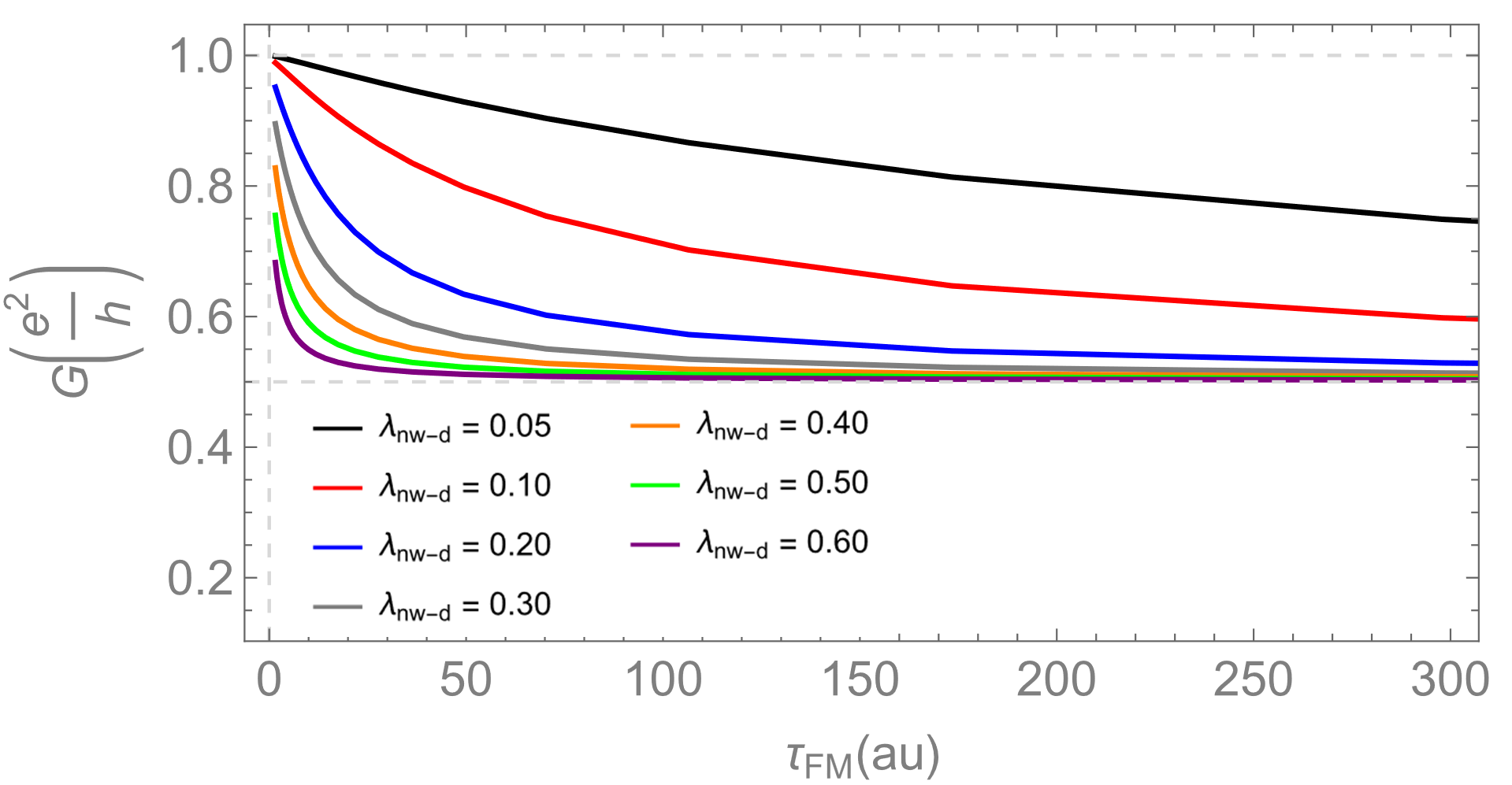
In order to better understand the conductance signal of the dissipative FMZMs, we show in Fig. 3 the values of $G$ as a function of FMZM lifetime $\tau_{FM}$ for different $\lambda_{nw-d}$. By increasing the strength $A$ of the Floquet drive (and shortening the FMZM lifetime $\tau_{FM}$) we find a transition between $G=e^{2}/2h$, indicating the presence of a Floquet Majorana mode, to $G=e^{2}/h$, which is the conductance of an uncoupled dot resonant at zero energy. A stronger coupling stabilizes the conductance signal around the Majorana signature $G=e^{2}/2h$. In the following, we start from the simplest toy model for dissipative Majorana modes in order to better analyze the numerical results.

A setting in which the undesired coupling could happen is the case in which the nanowire-dot coupling gets too large, the coupling of states above the induced gap can affect the value of the conductance. For instance, this effect can manifest itself when engineering very short FMZMs’ lifetimes, corresponding to larger amplitudes in the drive, as explained in section II.B and as established in [65]: in such a case, the spectrum in the nanowire is broadened and the SC gap derived from the Floquet GF becomes soft [64]. The effect on the conductance is shown in Fig. 5(a), where we modify our model parameters and we set some $\lambda_{nw-d}\gtrsim\Delta_{ind}$: the numerical results show values $G<e^{2}/2h$ when approaching shorter FMZM lifetimes. However, these conductance curves show a minimum for small $\tau_{FM}$, reverting to $G\rightarrow e^{2}/h$ for $\tau_{FM}\rightarrow 0$. A value of $G=0$ is a signature of a dot coupled to a normal fermion: Hence, the features seen in the figure are probably due to the contribution of states above the induced gap, detected via the strong coupling. However, since such quasiparticles also acquire a finite lifetime due to the drive and dissipation, the limit $G(\tau\rightarrow 0)=e^{2}/h$ should be maintained.

To analyze this behavior, we add to the MZM a normal fermion with finite width $\Gamma_{f}(\omega)$ and with finite energy $\delta$ –slightly off-resonant with the QD– to the MZM toy model. Hence, the GF becomes –in particle-hole space–

In order to derive the simplest possible expression for $G$ capturing the numerics, we make the following assumptions: The lifetimes of both the MZM and the off-resonant fermion are set to be the same $\Gamma_{f}=\Gamma_{M}\sim 1/\tau_{M}$, as well as the nanowire-QD coupling $\lambda_{nw-d}$. This leads to the following expression for the conductance (always with $\epsilon_{d}=0$):

A plot of the above function is shown in Fig. 5(b): The model is able to replicate the small-$\tau_{M}$/large-$\lambda$ features of the numerical simulation of 5(a), which we can now explain as follows: On the one hand, the FMZM’s lifetime is reduced by dissipation, leading to a reduced “effective coupling” $\tilde{\lambda}$ to the dot. On the other hand, the effect of SC gap softening in the nanowire as the amplitude of the periodic drive is increased can lead to a signal $G\rightarrow 0$ as the dot starts coupling to a normal fermion above the gap. This effect only becomes important as the nanowire-QD coupling $\lambda_{nw-dot}\gtrsim\Delta_{ind}$.

References

- Read and Green [2000] N. Read and D. Green, Phys. Rev. B 61, 10267 (2000).
- Kitaev [2001] A. Y. Kitaev, Physics-Uspekhi 44, 131 (2001).
- Kitaev [2003] A. Y. Kitaev, Annals of Physics 303, 2 (2003).
- Nayak et al. [2008] C. Nayak, S. H. Simon, A. Stern, M. Freedman, and S. Das Sarma, Rev. Mod. Phys. 80, 1083 (2008).
- Leinaas and Myrheim [1977] J. M. Leinaas and J. Myrheim, Il Nuovo Cimento B (1971-1996) 37, 1 (1977).
- Fredenhagen et al. [1989] K. Fredenhagen, K.-H. Rehren, and B. Schroer, Communications in Mathematical Physics 125, 201 (1989).
- Ivanov [2001] D. A. Ivanov, Phys. Rev. Lett. 86, 268 (2001).
- Sau et al. [2010] J. D. Sau, R. M. Lutchyn, S. Tewari, and S. Das Sarma, Phys. Rev. Lett. 104, 040502 (2010).
- Lutchyn et al. [2010] R. M. Lutchyn, J. D. Sau, and S. Das Sarma, Phys. Rev. Lett. 105, 077001 (2010).
- Oreg et al. [2010] Y. Oreg, G. Refael, and F. von Oppen, Phys. Rev. Lett. 105, 177002 (2010).
- Alicea [2010] J. Alicea, Phys. Rev. B 81, 125318 (2010).
- Alicea [2012] J. Alicea, Reports on Progress in Physics 75, 076501 (2012).
- Mourik et al. [2012] V. Mourik, K. Zuo, S. M. Frolov, S. Plissard, E. P. Bakkers, and L. P. Kouwenhoven, Science 336, 1003 (2012).
- Deng et al. [2012] M. Deng, C. Yu, G. Huang, M. Larsson, P. Caroff, and H. Xu, Nano letters 12, 6414 (2012).
- Das et al. [2012] A. Das, Y. Ronen, Y. Most, Y. Oreg, M. Heiblum, and H. Shtrikman, Nature Physics 8, 887 (2012).
- Churchill et al. [2013] H. O. H. Churchill, V. Fatemi, K. Grove-Rasmussen, M. T. Deng, P. Caroff, H. Q. Xu, and C. M. Marcus, Phys. Rev. B 87, 241401 (2013).
- Finck et al. [2013] A. D. K. Finck, D. J. Van Harlingen, P. K. Mohseni, K. Jung, and X. Li, Phys. Rev. Lett. 110, 126406 (2013).
- Albrecht et al. [2016] S. M. Albrecht, A. P. Higginbotham, M. Madsen, F. Kuemmeth, T. S. Jespersen, J. Nygård, P. Krogstrup, and C. Marcus, Nature 531, 206 (2016).
- Deng et al. [2016] M. Deng, S. Vaitiekėnas, E. B. Hansen, J. Danon, M. Leijnse, K. Flensberg, J. Nygård, P. Krogstrup, and C. M. Marcus, Science 354, 1557 (2016).
- Zhang et al. [2017a] H. Zhang, Ö. Gül, S. Conesa-Boj, M. P. Nowak, M. Wimmer, K. Zuo, V. Mourik, F. K. De Vries, J. Van Veen, M. W. De Moor, et al., Nature communications 8, 1 (2017a).
- Gül et al. [2018] Ö. Gül, H. Zhang, J. D. Bommer, M. W. de Moor, D. Car, S. R. Plissard, E. P. Bakkers, A. Geresdi, K. Watanabe, T. Taniguchi, et al., Nature nanotechnology 13, 192 (2018).
- Zhang et al. [2021] H. Zhang, M. W. de Moor, J. D. Bommer, D. Xu, G. Wang, N. van Loo, C.-X. Liu, S. Gazibegovic, J. A. Logan, D. Car, et al., arXiv preprint arXiv:2101.11456 (2021).
- Wang et al. [2022a] Z. Wang, H. Song, D. Pan, Z. Zhang, W. Miao, R. Li, Z. Cao, G. Zhang, L. Liu, L. Wen, R. Zhuo, D. E. Liu, K. He, R. Shang, J. Zhao, and H. Zhang, Phys. Rev. Lett. 129, 167702 (2022a).
- Wang et al. [2022b] Z. Wang, S. Zhang, D. Pan, G. Zhang, Z. Xia, Z. Li, D. Liu, Z. Cao, L. Liu, L. Wen, D. Liao, R. Zhuo, Y. Li, D. E. Liu, R. Shang, J. Zhao, and H. Zhang, Phys. Rev. B 106, 205421 (2022b).
- Song et al. [2022] H. Song, Z. Zhang, D. Pan, D. Liu, Z. Wang, Z. Cao, L. Liu, L. Wen, D. Liao, R. Zhuo, D. E. Liu, R. Shang, J. Zhao, and H. Zhang, Phys. Rev. Res. 4, 033235 (2022).
- Aghaee et al. [2022] M. Aghaee et al., (2022), 10.48550/ARXIV.2207.02472.
- Eckardt [2017] A. Eckardt, Rev. Mod. Phys. 89, 011004 (2017).
- Oka and Kitamura [2019] T. Oka and S. Kitamura, Annual Review of Condensed Matter Physics 10, 387 (2019), https://doi.org/10.1146/annurev-conmatphys-031218-013423 .
- Rudner and Lindner [2020] M. S. Rudner and N. H. Lindner, Nature reviews physics 2, 229 (2020).
- Castro et al. [2022] A. Castro, U. De Giovannini, S. A. Sato, H. Hübener, and A. Rubio, Phys. Rev. Research 4, 033213 (2022).
- Lindner et al. [2011] N. H. Lindner, G. Refael, and V. Galitski, Nature Physics 7, 490 (2011).
- Kitagawa et al. [2011] T. Kitagawa, T. Oka, A. Brataas, L. Fu, and E. Demler, Phys. Rev. B 84, 235108 (2011).
- Dahlhaus et al. [2011] J. P. Dahlhaus, J. M. Edge, J. Tworzydło, and C. W. J. Beenakker, Phys. Rev. B 84, 115133 (2011).
- Jiang et al. [2011] L. Jiang, T. Kitagawa, J. Alicea, A. R. Akhmerov, D. Pekker, G. Refael, J. I. Cirac, E. Demler, M. D. Lukin, and P. Zoller, Phys. Rev. Lett. 106, 220402 (2011).
- Kitagawa et al. [2012] T. Kitagawa, M. A. Broome, A. Fedrizzi, M. S. Rudner, E. Berg, I. Kassal, A. Aspuru-Guzik, E. Demler, and A. G. White, Nature communications 3, 1 (2012).
- Reynoso and Frustaglia [2013] A. A. Reynoso and D. Frustaglia, Phys. Rev. B 87, 115420 (2013).
- Liu et al. [2013] D. E. Liu, A. Levchenko, and H. U. Baranger, Phys. Rev. Lett. 111, 047002 (2013).
- Iadecola et al. [2013] T. Iadecola, D. Campbell, C. Chamon, C.-Y. Hou, R. Jackiw, S.-Y. Pi, and S. V. Kusminskiy, Phys. Rev. Lett. 110, 176603 (2013).
- Fregoso et al. [2013] B. M. Fregoso, Y. H. Wang, N. Gedik, and V. Galitski, Phys. Rev. B 88, 155129 (2013).
- Iadecola et al. [2014] T. Iadecola, T. Neupert, and C. Chamon, Phys. Rev. B 89, 115425 (2014).
- Foa Torres et al. [2014] L. E. F. Foa Torres, P. M. Perez-Piskunow, C. A. Balseiro, and G. Usaj, Phys. Rev. Lett. 113, 266801 (2014).
- Sedrakyan et al. [2015] T. A. Sedrakyan, V. M. Galitski, and A. Kamenev, Phys. Rev. Lett. 115, 195301 (2015).
- Rechtsman et al. [2013] M. C. Rechtsman, J. M. Zeuner, Y. Plotnik, Y. Lumer, D. Podolsky, F. Dreisow, S. Nolte, M. Segev, and A. Szameit, Nature 496, 196 (2013).
- Potter et al. [2016] A. C. Potter, T. Morimoto, and A. Vishwanath, Phys. Rev. X 6, 041001 (2016).
- Roy and Harper [2017] R. Roy and F. Harper, Phys. Rev. B 96, 155118 (2017).
- Bomantara and Gong [2018a] R. W. Bomantara and J. Gong, Phys. Rev. Lett. 120, 230405 (2018a).
- Bomantara and Gong [2018b] R. W. Bomantara and J. Gong, Phys. Rev. B 98, 165421 (2018b).
- Peng and Refael [2018] Y. Peng and G. Refael, Phys. Rev. B 98, 220509 (2018).
- Wang et al. [2013] Y. H. Wang, H. Steinberg, P. Jarillo-Herrero, and N. Gedik, Science 342, 453 (2013), https://www.science.org/doi/pdf/10.1126/science.1239834 .
- Mahmood et al. [2016] F. Mahmood, C.-K. Chan, Z. Alpichshev, D. Gardner, Y. Lee, P. A. Lee, and N. Gedik, Nature Physics 12, 306 (2016).
- Aeschlimann et al. [2021] S. Aeschlimann, S. A. Sato, R. Krause, M. Chávez-Cervantes, U. De Giovannini, H. Hübener, S. Forti, C. Coletti, K. Hanff, K. Rossnagel, A. Rubio, and I. Gierz, Nano Letters, Nano Letters 21, 5028 (2021).
- Mori et al. [2016] T. Mori, T. Kuwahara, and K. Saito, Phys. Rev. Lett. 116, 120401 (2016).
- Abanin et al. [2017a] D. A. Abanin, W. De Roeck, W. W. Ho, and F. m. c. Huveneers, Phys. Rev. B 95, 014112 (2017a).
- Abanin et al. [2017b] D. Abanin, W. De Roeck, W. W. Ho, and F. Huveneers, Communications in Mathematical Physics 354, 809 (2017b).
- Ponte et al. [2015] P. Ponte, A. Chandran, Z. Papić, and D. A. Abanin, Annals of Physics 353, 196 (2015).
- von Keyserlingk and Sondhi [2016] C. W. von Keyserlingk and S. L. Sondhi, Phys. Rev. B 93, 245145 (2016).
- Zhang et al. [2017b] J. Zhang, P. W. Hess, A. Kyprianidis, P. Becker, A. Lee, J. Smith, G. Pagano, I.-D. Potirniche, A. C. Potter, A. Vishwanath, et al., Nature 543, 217 (2017b).
- Choi et al. [2017] S. Choi, J. Choi, R. Landig, G. Kucsko, H. Zhou, J. Isoya, F. Jelezko, S. Onoda, H. Sumiya, V. Khemani, et al., Nature 543, 221 (2017).
- Bauer et al. [2019] B. Bauer, T. Pereg-Barnea, T. Karzig, M.-T. Rieder, G. Refael, E. Berg, and Y. Oreg, Phys. Rev. B 100, 041102 (2019).
- Hone et al. [2009] D. W. Hone, R. Ketzmerick, and W. Kohn, Phys. Rev. E 79, 051129 (2009).
- Iadecola et al. [2015] T. Iadecola, T. Neupert, and C. Chamon, Phys. Rev. B 91, 235133 (2015).
- Liu [2015] D. E. Liu, Phys. Rev. B 91, 144301 (2015).
- Seetharam et al. [2015] K. I. Seetharam, C.-E. Bardyn, N. H. Lindner, M. S. Rudner, and G. Refael, Phys. Rev. X 5, 041050 (2015).
- Yang et al. [2021a] Q. Yang, Z. Yang, and D. E. Liu, Phys. Rev. B 104, 014512 (2021a).
- Yang et al. [2021b] Z. Yang, Q. Yang, J. Hu, and D. E. Liu, Phys. Rev. Lett. 126, 086801 (2021b).
- Liu et al. [2017] D. E. Liu, A. Levchenko, and R. M. Lutchyn, Phys. Rev. B 95, 115303 (2017).
- Liu and Baranger [2011] D. E. Liu and H. U. Baranger, Phys. Rev. B 84, 201308 (2011).
- Kells et al. [2012] G. Kells, D. Meidan, and P. W. Brouwer, Phys. Rev. B 86, 100503 (2012).
- Moore et al. [2018a] C. Moore, T. D. Stanescu, and S. Tewari, Phys. Rev. B 97, 165302 (2018a).
- Moore et al. [2018b] C. Moore, C. Zeng, T. D. Stanescu, and S. Tewari, Phys. Rev. B 98, 155314 (2018b).
- Vuik et al. [2019] A. Vuik, B. Nijholt, A. R. Akhmerov, and M. Wimmer, SciPost Phys. 7, 061 (2019).
- Liu et al. [2021] D. Liu, Z. Cao, X. Liu, H. Zhang, and D. E. Liu, Phys. Rev. B 104, 205125 (2021).
- Pan and Das Sarma [2020] H. Pan and S. Das Sarma, Phys. Rev. Research 2, 013377 (2020).
- Shtanko and Movassagh [2020] O. Shtanko and R. Movassagh, Phys. Rev. Lett. 125, 086804 (2020).
- Liu et al. [2015] D. E. Liu, M. Cheng, and R. M. Lutchyn, Phys. Rev. B 91, 081405 (2015).
- Kamenev [2011] A. Kamenev, Field Theory of Non-Equilibrium Systems (Cambridge University Press, 2011).
- Altland and Simons [2010] A. Altland and B. D. Simons, Condensed Matter Field Theory, 2nd ed. (Cambridge University Press, 2010).
- Haug et al. [2008] H. Haug, A.-P. Jauho, et al., Quantum kinetics in transport and optics of semiconductors, Vol. 2 (Springer, 2008).