Chiral edge waves in a dance-based human topological insulator
Topological insulators are insulators in the bulk but feature chiral energy propagation along the boundary. This property is topological in nature and therefore robust to disorder. Originally discovered in electronic materials, topologically protected boundary transport has since been observed in many other physical systems. Thus, it is natural to ask whether this phenomenon finds relevance in a broader context. We choreograph a dance in which a group of humans, arranged on a square grid, behave as a topological insulator. The dance features unidirectional flow of movement through dancers on the lattice edge. This effect persists when people are removed from the dance floor. Our work extends the applicability of wave physics to the performance arts.
A topological property of an object is one that is unchanged as the object undergoes continuous deformation, which includes translation, rotation, stretching/compression, and bending but excludes puncturing, tearing, and gluing (together different parts of it). More than just a theoretical concept, this notion can have real-life applications. Consider a physical material with a topological property. The latter is resistant to material imperfections that constitute continuous deformations (though not necessarily in real space). Due to this robustness, such materials, which are known as topological materials, have garnered widespread attention over the past several decades [1, 2, 3].
To date, the most studied topological material has been the topological insulator [1]. A topological insulator is insulating in the bulk but conducting on the boundary. The earliest known topological insulators are two-dimensional electronic materials that exhibit the integer quantum Hall effect [4], in which the (transverse Hall) conductance along the sample edge is proportional to a nonzero integer . Reflecting the net number of edge states that support clockwise (or counterclockwise) current, and thus the edge conductance are topological properties [5]. Remarkably, these characteristics of the edge are intimately related to properties of the material bulk. Such bulk-boundary correspondence is a hallmark of topological insulators.
Since their discovery, topological insulators have been observed in a plethora of other physical media. Examples include traditional wave media, both natural (e.g., oceanic and atmospheric fluids [6]) and synthetic (e.g., photonic [7, 8] and acoustic [9, 10] lattices). Topological insulators have also been reported in settings that have less in common with electronic materials: systems governed by Newton’s equations of motion [11, 12, 10], amorphous materials [13], active matter [14, 15, 16], and stochastic processes [17, 15, 18].
The ubiquity of topological insulators prompts the question of whether their physics can manifest in contexts that transcend the usual boundaries of science. In this work, we present a human topological insulator in the form of a group dance. Functioning literally as a numerical integrator of the time-dependent Schrödinger equation (TDSE), the dance features chiral motion through people along the edge of the dance floor, even when “defects” are introduced by removing dancers. In essence, this dance is distinct from those that serve as natural examples or purely qualitative representations of concepts in science and math (including seismic waves [19], electrical circuits [20], and topology [21]). Thus, the dance described in this article serves both as a rigorous realization of topological edge modes as well as an ideal outreach activity to introduce broader audiences to the universal concepts of topological protection.
To begin the choreography, we consider the Harper-Hofstadter Hamiltonian [22, 23] with next-nearest neighbor (NNN) coupling [24] and magnetic flux per plaquette (Fig. 1A),
| (1) |
which models an electron hopping on a square lattice in a magnetic field. The lattice sites are labeled by , and ( here) is the magnitude of intersite coupling. Hops to a nearest neighbor (NN) occur with an amplitude of , while hops to a NNN occur with an amplitude of . Here, H.c. stands for Hermitian conjugate.
The Hamiltonian gives rise to several dynamical features that are characteristic of topological insulators, as shown by simulations on a finite lattice [25]. When exciting an edge site of a square-shaped lattice, the excitation propagates clockwise along the edge (Fig. 1B and Movie S1). This chiral transport persists after introducing lattice defects of various shapes (Fig. 1C and Movie S2). For a lattice with a hole in the middle, which is known as the Corbino geometry [26, 27], an excitation at the inner edge moves along this edge with opposite handedness, i.e., counterclockwise (Fig. 1D and Movie S3). The unidirectional conduction on the edges is drastically different from the dynamics in the bulk, in which a localized excitation diffuses with little directional selectivity (Fig. 1E and Movie S4).
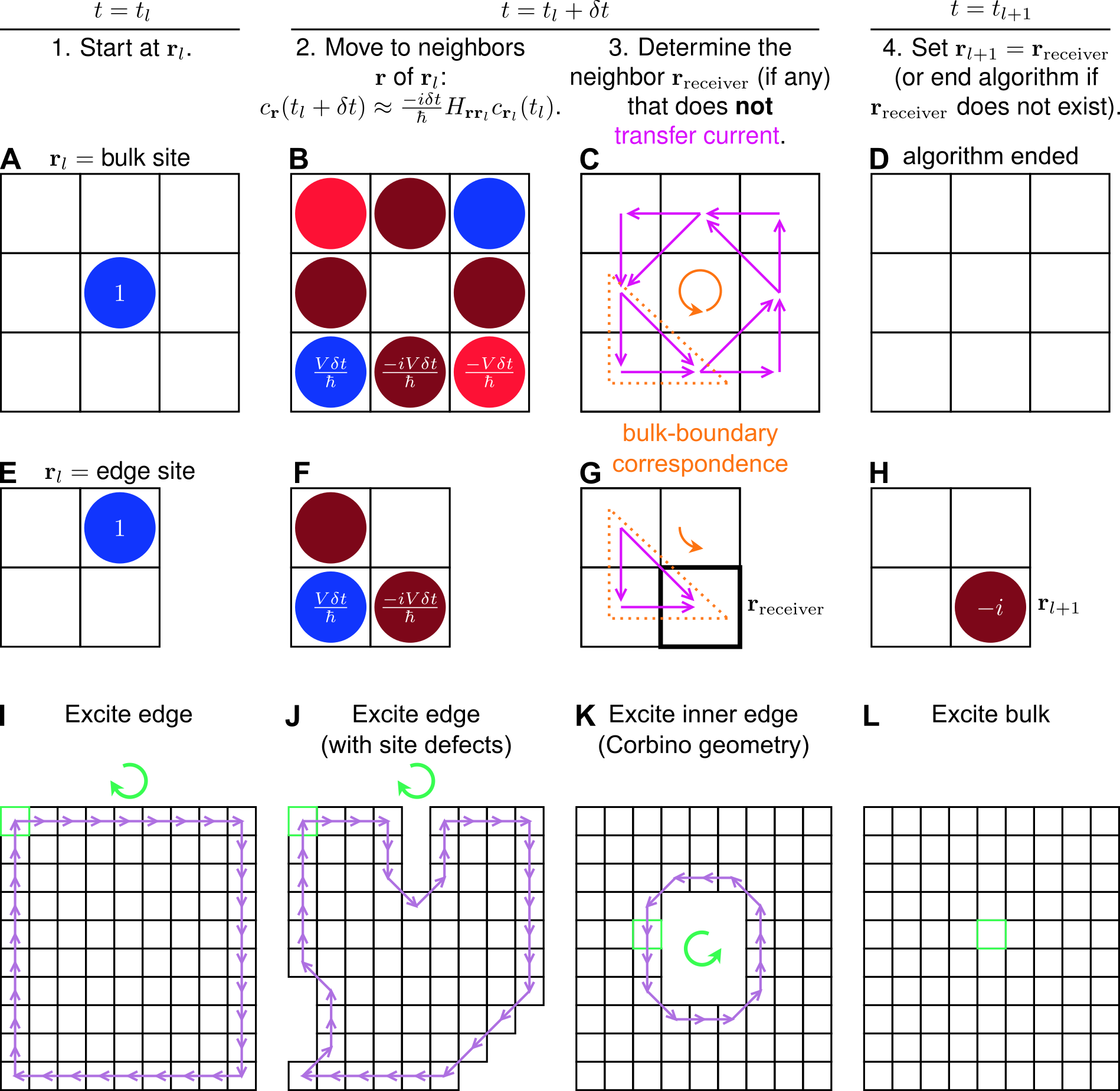
To capture such dynamics in a dance, we first present an algorithm to (approximately) propagate the wavefunction in discrete time. The algorithm goes as follows (Fig. 2, A to H):
- 1.
- 2.
Evolve the wavefunction forward by time , and approximate the resulting state up to :
(4) where is the set of neighbors (NN and NNN) of (Fig. 2, B and F).
- 3.
- 4.
Crucial to the algorithm are Steps 3 and 4, during which the probability amplitudes interfere, ultimately localizing at . This makes intuitive sense, since is the “attractor/sink” of the current field at time (Step 3, Fig. 2G). We have assumed that there is at most one neighbor of , which is true for the lattice geometries appearing in this work [see supplementary materials (SM) Section 2].
In Fig. 2, I to L, we show the dynamics generated by the algorithm. The results are in excellent qualitative agreement with the exact dynamics (Fig. 1, B to E, respectively; see also Movies S1-S4, respectively). Notably, the algorithm reproduces the confinement of an edge excitation to the edge, the chirality with which this excitation moves, and the robustness of these properties to site defects. Also captured is the diagonal movement of an edge excitation as it travels around the defects (cf. Figs. 2J and 1C) and, in the Corbino geometry, past the corners of the inner edge (cf. Figs. 2K and 1D).
Underlying the high qualitative accuracy of Algorithm 1 is the direct dependence of the dynamics on the site currents. For an iteration starting at a bulk site (Fig. 2A), current flows to and from all neighbors of the initial site (Fig. 2C). As a result, the algorithm ends (Fig. 2, D and L), reflecting the absence of unidirectional propagation in the bulk. Interestingly though, the current vectors form a vortex with a well-defined chirality (i.e., counterclockwise; see Fig. 2C, purple arrows). By considering an appropriate subset of this current field (Fig. 2C, orange dotted triangle), one can obtain the current field for an iteration beginning at an edge (Fig. 2G, orange dotted triangle). This subfield (Fig. 2G, purple arrows) determines the site that the wavefunction will occupy at the start of the next iteration (Fig. 2H). Thus, the currents of a bulk-localized wavefunction indicate how an edge-localized wavefunction would propagate. In particular, the subset relation between edge and bulk current fields (Fig. 2, G and C, orange dotted triangles), and the structure of the latter (Fig. 2C, purple arrows), explain why edge excitations are confined to the edge. Furthermore, the chirality of the bulk currents (Fig. 2C, orange arrow) is directly correlated with the chirality of the edge dynamics (Fig. 2G, orange arrow). These properties constitute a dynamical form of bulk-boundary correspondence. In particular, they closely resemble the classical picture of an electron in a magnetic field, where the circular orbits of a free particle manifest as unidirectional skipping motion along an edge [1].
To convert the algorithm to a dance, it is useful to transform the wavefunction from the complex plane to the real numbers. To see that this transformation is possible, notice that, at all times explicitly considered in the algorithm (i.e., ), the probability amplitude at each satisfies
| (6) |
This property results from the choice of initial state (Eq. 3), which depends on whether is even or odd; the update rule of Step 4 (Eq. 4); and the structure of the Hamiltonian (Eq. 1), which has purely real NN couplings and purely imaginary NNN couplings. Moreover, since all hopping amplitudes have the same magnitude (Eq. 1), for all neighboring sites of . It follows that only the signs of these coefficients are necessary to capture the essential physics, where the signs are given by
| (7) |
Thus, applying to all probability amplitudes recasts the algorithm in terms of real numbers (SM Section 3), i.e., the transformed amplitudes and “effective Hamiltonian”
| (8) |
By definition, and each takes the values . We emphasize that the site probabilities at times , and hence the overall dynamics, remain unchanged from the original algorithm.
We proceed to choreograph a dance via a direct mapping of the reformulated algorithm. The probability amplitudes are represented by dance moves:
| (9) |
“Up” and “down” refer to the waving of flags with arms pointed in the indicated direction (Fig. 3B, blue and red, respectively). In contrast, “stand still” is exactly as the name suggests, with arms relaxed at the sides of the dancer (Fig. 3B, gray). The (nonzero) hopping amplitudes are represented as
| (10) |
The above redefinitions result in the following rules for multiplying the probability amplitudes with the hopping amplitudes:
| (11) |
With this “human representation” of the wavefunction and “effective Hamiltonian” , the real-valued algorithm is readily converted to a dance, described as follows. The dance floor (Fig. 3A) is a finite square grid, where the squares contain blue and red lines. Each square represents a lattice site . The blue/red lines within that square represent the amplitudes = same/opposite of hopping to neighboring sites (Fig. 3A, zoom-in). For each site that the electron can occupy, a dancer is placed in the corresponding square. Given this setup, the dance is performed in rounds, where each round has the steps below (Fig. 3D):
- (Command)
The person designated as the commander is dancing up or down. The commander tells each neighbor to dance in the same or opposite way, according to the line in the commander’s square that points to this neighbor (Fig. 3D, leftmost panel, circled lines). The neighbors start dancing as commanded.
- (Command-to-Match transition)
The commander stands still.
- (Match)
Within the neighbors of the commander, each person scans across the others, looking for a match. As demonstrated in Fig. 3C, the person at matches with the person at if the dance move of the former, times , equals the dance move of the latter, where is given by the line in square that points to square .
- (Match-to-Command transition)
All people with a match stop dancing. If there is a person without a match, this person continues dancing and becomes the commander; return to the Command step. If everyone has a match, the dance ends.
The Command step (equivalent to Step 2 of the algorithm) represents the spreading of a localized wavefunction to neighboring sites. The probability amplitudes at these sites interfere during the Match step (equivalent to Step 3 of the algorithm) and Match-to-Command transition (equivalent to Step 4 of the algorithm). Rather than having to memorize the values of for Command and Match, the dancers simply consult the blue and red lines in their respective squares.
As a science outreach event, we taught the dance to students at Orange Glen High School in Escondido, California [25]. Overall, the students mastered the dance steps (Fig. 4A) in under one hour. The students (plus some of us) then performed the dance for various initial conditions and lattice geometries [25]. To engage more students, some performances began with two people dancing (as commander) on the same dance floor; two independent dances ensued simultaneously (see, for example, Fig. 4B and Movie S5) for all but one dance round (see below). The performances display key dynamical features of topological insulators, namely, those generated by the algorithm on which the choreography is based. When the initial dancers are at an edge, the dancing propagates unidirectionally along this edge: clockwise on the outer edge of a square-shaped lattice (Fig. 4B and Movie S5) and counterclockwise on the inner edge of a lattice with Corbino geometry (Fig. 4D and Movie S7). For the former lattice, we introduced site defects by removing people at the edge of the dance floor. Still, the lattice sustains an edge-confined and clockwise-oriented “dance wave,” which maneuvers around the vacancies (Fig. 4C and Movie S6) and even persists through the interference of two concurrent dances (Movie S6) . As expected (Fig. 2L), the dance only lasts one round when an initial dancer is in the bulk (Fig. 4E and Movie S8).
In summary, we have choreographed a dance in which a group of people behave as a topological insulator. The choreography involves developing an algorithm for approximate wavefunction propagation and mapping the wavefunction first to the real numbers and then to human movements. The resulting dance, which operates as a numerical integrator of the TDSE, exhibits the salient dynamics of topological insulators. This work provides a blueprint for creating a classical simulator of topological insulators. Achieving this task for additional Hamiltonians would mark an intriguing and unique frontier at the interface of wave physics, science education, and performance arts.
References
- [1] M. Z. Hasan, C. L. Kane, Rev. Mod. Phys. 82, 3045 (2010).
- [2] X.-L. Qi, S.-C. Zhang, Rev. Mod. Phys. 83, 1057 (2011).
- [3] B. Yan, C. Felser, Annu. Rev. Condens. Matter Phys. 8, 337 (2017).
- [4] K. von Klitzing, G. Dorda, M. Pepper, Phys. Rev. Lett. 45, 494 (1980).
- [5] D. J. Thouless, M. Kohmoto, M. P. Nightingale, M. den Nijs, Phys. Rev. Lett. 49, 405 (1982).
- [6] P. Delplace, J. B. Marston, A. Venaille, Science 358, 1075 (2017).
- [7] Z. Wang, Y. Chong, J. D. Joannopoulos, M. Soljac̆ić, Nature 461, 772 (2009).
- [8] L. Lu, J. D. Joannopoulos, M. Soljac̆ić, Nat. Photonics 8, 821 (2014).
- [9] C. He, et al., Nat. Phys. 12, 1124 (2016).
- [10] G. Ma, M. Xiao, C. T. Chan, Nat. Rev. Phys. 1, 281 (2019).
- [11] R. Süsstrunk, S. D. Huber, Science 349, 47 (2015).
- [12] L. M. Nash, et al., Proc. Natl. Acad. of Sci. USA 112, 14495 (2015).
- [13] N. P. Mitchell, L. M. Nash, D. Hexner, A. M. Turner, W. T. M. Irvine, Nat. Phys. (2018).
- [14] S. Shankar, M. J. Bowick, M. C. Marchetti, Phys. Rev. X 7, 031039 (2017).
- [15] K. Dasbiswas, K. K. Mandadapu, S. Vaikuntanathan, Proc. Natl. Acad. Sci. USA 115, E9031 (2018).
- [16] S. Shankar, A. Souslov, M. J. Bowick, M. C. Marchetti, V. Vitelli, Nat. Rev. Phys. 4, 380 (2022).
- [17] A. Murugan, S. Vaikuntanathan, Nat. Commun. 8, 13881 (2017).
- [18] E. Tang, J. Agudo-Canalejo, R. Golestanian, Phys. Rev. X 11, 031015 (2021).
- [19] K. Miller, Demonstrating P and S Seismic Waves, \urlhttps://www.youtube.com/watch?v=gjRGIpP-Qfw&ab%005Fchannel=KeithMiller (2012).
- [20] NOVA PBS Official, How Dancing Can Help You Learn Science, \urlhttps://www.youtube.com/watch?v=d-7AZprW0Rw&ab%005Fchannel=NOVAPBSOfficial (2016).
- [21] G. M. Graf, Bulk-edge duality for topological insulators, presented at Quantum Spectra and Transport, Jerusalem, Israel, 30 June - 4 July, 2013, \urlhttp://math.huji.ac.il/%7Eavronfest/Graf.pdf.
- [22] P. G. Harper, Proc. Phys. Soc. Lond. A 68, 874 (1955).
- [23] D. R. Hofstadter, Phys. Rev. B 14, 2239 (1976).
- [24] Y. Hatsugai, M. Kohmoto, Phys. Rev. B 42, 8282 (1990).
- [25] Materials and methods are available as supplementary materials at the Science website.
- [26] O. M. Corbino, Atti R. Accad. Lincei 20, 342 (1911).
- [27] B. I. Halperin, Phys. Rev. B 25, 2185 (1982).
- [28] H. U. Baranger, D. P. DiVincenzo, R. A. Jalabert, A. D. Stone, Phys. Rev. B 44, 10637 (1991).
- [29] T. N. Todorov, J. Phys.: Condens. Matter 14, 3049 (2002).
Acknowledgments
M.D. would like to thank Raphael Ribeiro for discussions on topological insulators at the beginning of this project. We are grateful to the UCSD Chem 126a Fall 2019 undergraduate students for participating in the trial lesson for a preliminary version of the dance, and to Luis Martínez-Martínez and Leonardo Calderón for helping run that trial lesson. We thank Madison Edwards, Hilliary Frank, Melanie Gonzalez, Etienne Palos, Richa Rashmi, Michael Reiss, Shubham Sinha, Luisa Andreuccioli, Benjamin Huang, and Clara van den Wildenberg for pariticipating in the practice lessons for the final version of the dance. Regarding the official dance performances, we are grateful to Dania Monroy and the students of D.K. for their participation. We thank Amy Booth, Shannon Chamberlin, and Susan Yonezawa for their help in organizing the outreach event.
Funding
The scientific and outreach components of this work were funded by the NSF Grant No. CAREER CHE 1654732.
Author contributions
J.Y.-Z. conceptualized and supervised the study. M.D. designed the wavefunction propagation algorithms and ran simulations. M.D. choreographed the dance, with input from J.B.P.-S., J.A.C.-G.-A., A.K., F.M., S.P.-S., Y.R.P., K. Schwennicke, K. Sun, S.v.d.W., and J.Y.-Z. M.D., D.K., A.B., and J.Y.-Z. organized the outreach event. M.D., J.B.P.-S., J.A.C.-G.-A., A.K., F.M., S.P.-S., Y.R.P., K. Schwennicke, K. Sun, S.v.d.W., J.Y.-Z., and D.K. ran the event. J.B.P.-S. and S.v.d.W. took pictures and recorded videos of the dance lessons and performances. M.D. and J.B.P.-S. analyzed the dance performances. M.D. and J.Y.-Z. wrote the manuscript.
Competing interests
The authors declare no competing interests.
Data and materials availability
All data are available in the main text or the supplementary materials.
Supplementary materials
Materials and Methods
Supplementary Text
Figs. S1 to S5
Movies S1 to S8



Supplementary Materials for
This PDF file includes:
Materials and Methods
Supplementary Text
Figs. S1 to S5
Other Supplementary Material for this manuscript
includes the following:
Movies S1 to S8
Materials and Methods
Calculating the dynamics generated by
At time , the system is excited (i.e., initialized) at site , and the wavefunction is given by
| (S1) |
To calculate the wavefunction at later times, we first move to the eigenbasis:
| (S2) |
where is the eigenstate of with energy . We then calculate the wavefunction at time as
| (S3) |
Changing back to the position basis,
| (S4) |
we obtain the site probabilities . Fig. 1, B to E, and Movies S1-S4 plot the site probabilities as a function of time using a time step of 0.1 .
Science outreach: topological dance
In this section, we describe the science outreach event at Orange Glen High School on April 27, 2022, in which we taught the dance to its students. A dance lesson was held during each of three physics classes in lieu of the normal class activities. In the lesson, students learned, practiced, and performed the dance. The lesson took most of the class period, which was 100 minutes long. Since class sizes were around 20 or less, we (the school teachers and dance instructors) joined the students in the dance performances. We recommend that the dance be carried out with at least 25 people, so that the human lattice has a well-defined bulk (i.e., people who will never dance up or down if the initial dancers are at the edge).
Before the lesson, we set up (Fig. S1A) a big dance floor (6 6 square grid; Figs. S1B and S2A) and several small dance floors (2 2 square grid; Figs. S1C and S2C). The dance floors had grid lines made of beige masking tape (1” thick) and squares measuring approximately 1 m 1 m (Fig. S2). Pieces of blue and red painters tape (1” thick and 4-10” long) were placed in each square according to the structure of “effective Hamiltonian” (Fig. S2; compare to Fig. 3A). In the big dance floor, the squares were enumerated from 1 to 36 (Fig. S1B and S2B) to assist in the execution of the dance performances (see below).


Following a brief introduction to topological insulators and the lesson, the students were divided into groups of 4. Each group moved to a practice dance floor, where one of us taught them the mechanics of the dance. The students first learned the dance moves. Fig. S3 shows what the dance moves look like in real life (see cartoon version in Fig. 3B). To make the moves more distinguishable, dancers are encouraged to cover their flags with their hands when doing “stand still” (Fig. S3B) and crouch when doing “down” (Fig. S3D). The students then learned the Command step. After each student had a chance to practice being commander, they learned the Match step. Finally, the students practiced both steps together (including the transitions between the steps) until mastery was achieved. Most students had mastered the dance steps after 30-45 minutes.

Next, the students moved to the main dance floor to rehearse and perform the dance for 2-3 sets of initial conditions (i.e., who the commanders are in the first round of the dance) and arrangements of students (e.g., square-shaped lattice, Corbino geometry). Accompanied by music, each performance proceeded as follows. We first called out the number(s) of the student(s) who would serve as the commanders in the first round of the dance. To begin the dance, we blew a whistle and announced “Command,” signaling for the assigned commanders to carry out Command. Once all neighbors of the commander(s) had begun dancing, we blew a whistle and announced “Match,” initiating the transition from Command to Match. After 15-20 seconds, which was enough for students to carry out Match, we blew a whistle and announced “Command” to switch to Command of the next round. This cycle was repeated for each round of the dance.
Supplementary Text
1 A useful property of the current operator
Consider the operator (see main text for definition) representing the current from to . With respect to wavefunction , the expectation value of this current is
| (S5) |
We use this property later in the supplementary text.
2 Cases when there are multiple sites
In the algorithm of the main text, we assume that there is at most one neighbor (NN or NNN) of that does not transfer current to another neighbor of . The assumption is true for the lattice geometries (e.g., square shaped, Corbino) employed in our simulations and dances. In this section, we discuss cases featuring multiple neighbors .
For a given , there are multiple sites when the neighbors of are a union of non-neighboring sets of sites (Fig. S4). Here, we denote sets of sites as non-neighboring if none of are neighbors for any . For a given lattice geometry, the presence of multiple sites can occur if a site and its neighbors form an arrangement of Fig. S4.

3 Algorithm 2: generating real-valued, discrete-time dynamics of a topological insulator
The algorithm in the main text, hereafter referred to as Algorithm 1, propagates the (complex-valued) wavefunction in discrete time for the model topological insulator with (complex-valued) Hamiltonian (Eq. 1). In this section, we present the algorithm that results from transforming the probability amplitudes according to , where is the real-valued function defined in Eq. 7. The transformed algorithm, hereafter referred to as Algorithm 2, is written in terms of real-valued quantities.
3.1 Algorithm 2
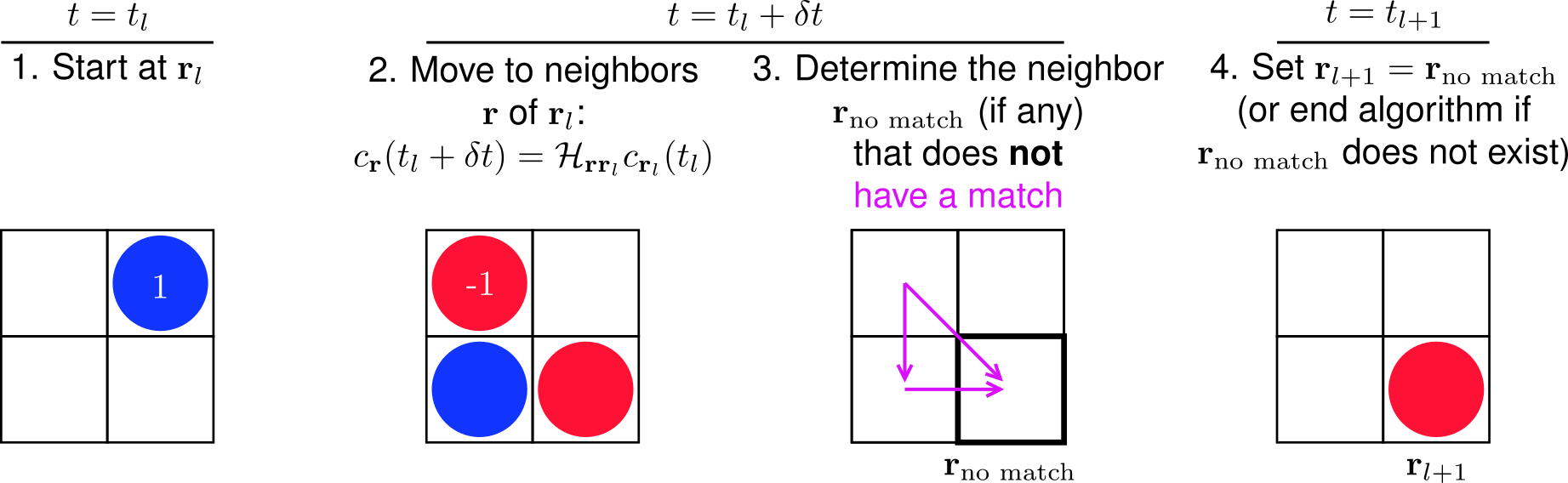
Here are the steps of Algorithm 2 (Fig. S5):
- 1.
At the th time step, , the wavefunction is at site :
(S6) - 2.
Evolve the wavefunction forward by time :
(S7) - 3.
Determine the neighbor (if any) of that does not match with another neighbor of . We say that matches with if the probability amplitude of the former equals that of the latter after multiplication by , i.e., .
- 4.
If there is a neighbor of , set
(S8) and ; return to Step 2. If not, the algorithm terminates.
3.2 Derivation of Algorithm 2
In this section, we show that applying (Eq. 7) to the probability amplitudes allows us to write each step of Algorithm 1 as the same step of Algorithm 2.
The derivation goes as follows:
- 1.
- 2.
Notice that (Eq. 1) has purely real NN couplings and purely imaginary NNN couplings, i.e.,
(S10) Using this equation, one can show that (see Eq. 4)
(S11) for . It follows that
(S12) where is defined in Eq. 8. Moreover, since (Eq. 4), then
(S13) Comparing Eqs. S12-S13 to Eq. S7 for of Algorithm 2, we see that applying to all converts Step 2 of Algorithm 1 to the same step of Algorithm 2.
- 3.
- 4.
Using
for all and renaming as ,we can rewrite Step 4 of Algorithm 1 as the same step of Algorithm 2.
Movie S1. Dynamics generated by for the parameters
used in Fig. 1B. The probability of the system being
at each site is represented by a circle (area probability).
Movie S2. Dynamics generated by for the parameters used
in Fig. 1C. The probability of the system being
at each site is represented by a circle (area probability).
Movie S3. Dynamics generated by for the parameters used
in Fig. 1D. The probability of the system being
at each site is represented by a circle (area probability).
Movie S4. Dynamics generated by for the parameters used
in Fig. 1E. The probability of the system being
at each site is represented by a circle (area probability).
Movie S5. The dance where the initial dancers are on the
lattice edge. Snapshots are shown in Fig. 4B.
Movie S6. The dance where the initial dancers are on the
edge of a lattice with site defects. Snapshots are shown in Fig. 4C.
Movie S7. The dance where the initial dancer is on the inner
edge of a lattice with a hole in the middle (i.e., Corbino geometry).
Snapshots are shown in Fig. 4D.
Movie S8. The dance where the initial dancer is in the lattice
bulk. Snapshots are shown in Fig. 4E.