quTARANG: A python GPE solver to study turbulence in quantum systems

Turbulence is a phenomenon associated with the chaotic nature of flows in space and time solely arising due to the nonlinear nature of the interactions. Turbulence in classical fluids, as best characterised by the Navier-Stokes equation, remains unresolved to this day. The complex nonlinear interactions at various length and time scales make it a difficult problem to handle analytically as well as numerically. One recent approach to shed some light on this long-standing problem has been the study of turbulence in quantum fluids. The zero viscosity and quantized vortices of quantum fluid systems like Bose-Einstein Condensates (BECs) [1] distinguish it from its classical counterparts. BEC is a state of matter where Bose particles occupy the ground state upon cooling to a very low temperature and thus can be represented by a macroscopic wave function. One can model the dynamics of BECs using the mean-field Gross-Pitaevskii Equation (GPE) given by [2]

where $\psi(\vec{r},t)$ is the macroscopic complex wave function, $m$ is the atomic mass, $V(\vec{r},t)$ is the trapping potential, $N$ is the number of particles, $\displaystyle U_{0}=(4\pi\hslash^{2}a_{s})/m$ is the nonlinear interaction parameter and $a_{s}$ denotes the scattering length for the interaction of the atomic particles.

Our quantum simulator code quTARANG¹¹ 1 github.com/sachinrawat2207/quTARANG is primarily designed for studying quantum turbulence in BECs by solving the GPE in laminar as well as in the turbulent regime.

quTARANG is a robust and easy-to-use application that solves the GPE with Graphics Processing Unit (GPU). GPUs are specialized units primarily designed for image processing and for performing massive multigrid simulations at high speed. They have a large number of parallelizing units compared to CPUs, due to which they are being widely used to speed up code. There are no packages available in python that can solve turbulent GPE in 2D and 3D on both CPUs and GPUs. There exist, however, some software packages in other languages that can solve the GPE such as GPELab [3], Massively Parallel Trotter-Suzuki Solver [4], CUDA-enabled GPUE [5], a split-step Crank-Nicolson based Fortran code [2] and MPI-OpenMP enabled Gross-Pitaevskii Solver (GPS) [6].

We have chosen the frequency ($\omega^{-1}$) as the time scale, oscillator length $a_{0}=\sqrt{\hbar/m\omega}$ as the characteristic length scale and the harmonic oscillator ground state energy $\hbar\omega$ as the energy scale. With this formalism, the non-dimensional variables can be written as $t^{\prime}=\omega t$, $\vec{r}^{\prime}=\vec{r}/a_{0}$ and $\psi^{\prime}=a_{0}^{3/2}\psi$. In what follows, we omit the prime $(^{\prime})$ from the variables. The non-dimensional form of the GPE is given by [2]

where $g$ is the non-dimensional interaction parameter.

quTARANG uses a pseudo-spectral scheme, Time-splitting spectral (TSSP) method [7], to solve the dynamics of the GPE. The main advantage of using the TSSP scheme is that it is unconditionally stable and conserves the total particle number.

The ground state calculations in quTARANG are done by using TSSP with an imaginary time propagation method. In this method, one replaces $t$ with $-it$. As we propagate in imaginary time, the eigenstates with higher energies begin to decay faster than the ground state as a result of which only the ground state survives. The wavefunction needs to be normalised at each time step in order to conserve total particle number.

quTARANG is equipped with various features, which include:

1. 1.

   Ground state calculations for different potentials such as harmonic and anharmonic trap, optical lattice potential, time-dependent potential and stochastic potential.

2. 2.

   Long-time dynamical evolution of different states using either CPUs or GPUs.

3. 3.

   Computation of different quantities relevant to the study of turbulence phenomenon in BECs, such as components of kinetic energy (KE) and various spectra (compressible KE spectrum, incompressible KE spectrum and particle number spectrum).

We have calculated the ground state and dynamics for given sets of initial conditions and compared them with the standard results.

1. 1.

   Validation of ground state : The initial condition for 2D and 3D cases are given as:

   2D : $\psi(\vec{r},0)=\left(\frac{1}{\pi}\right)^{1/2}e^{-\frac{(x^{2}+y^{2})}{2}}$,  $V(\vec{r})=\frac{1}{2}(x^{2}+y^{2})$

   3D : $\psi(\vec{r},0)=\left(\frac{1}{\pi}\right)^{3/4}e^{-\frac{(x^{2}+y^{2}+z^{2})}{2}}$,  $V(\vec{r})=\frac{1}{2}(x^{2}+y^{2}+4z^{2})$

   The ground state obtained by quTARANG has been compared with that obtained by using the finite difference code of Muruganandam and Adhikari [2]. The results for harmonic potential well for 2D and 3D are in good agreement with Muruganandam and Adhikari [2] as shown in Table 1. The root-mean-square size ($r_{rms}$) of the condensate is defined as $r_{rms}=\left(\int r^{2}|\psi(\vec{r},t)|^{2}dV\right)^{1/2}$.

2. 2.

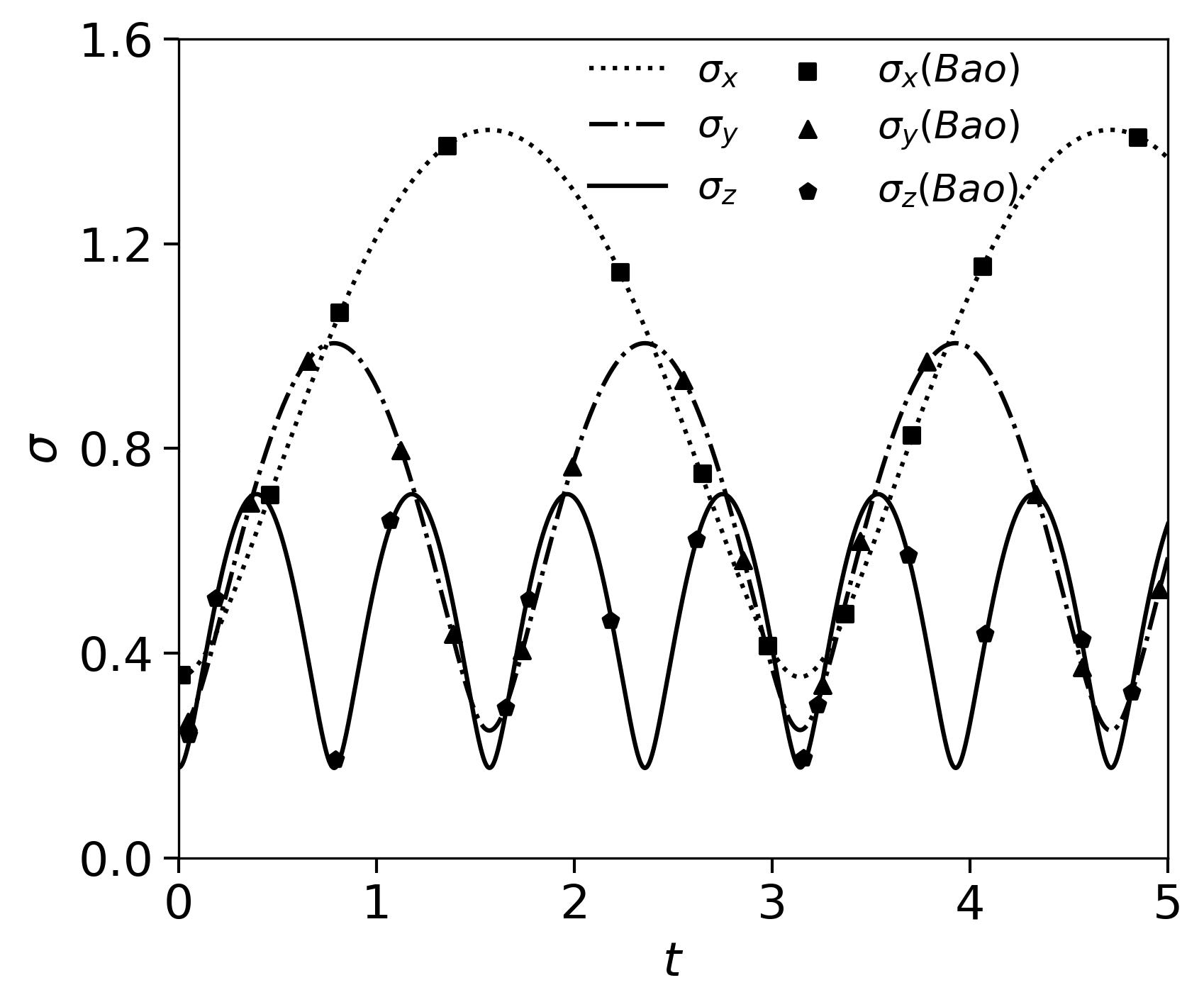
   Validation of dynamics : We have validated the dynamic evolution of a state by comparing our results with Bao et al. [7] for the following condition:

   $$\psi(\vec{r},0)=\frac{(\gamma_{y}\gamma_{z})^{1/4}}{\sqrt{(\pi\epsilon_{1})^{3/4}}}e^{-\frac{(x^{2}+\gamma_{y}y^{2}+\gamma_{z}z^{2})}{2\epsilon_{1}}},\ \ \ V(\vec{r},0)=\frac{1}{2}(x^{2}+\gamma_{y}^{2}y^{2}+\gamma_{z}^{2}z^{2}),$$

   where $\gamma_{y}=2.0$, $\gamma_{z}=4.0$, $\epsilon_{1}=0.25$ and $g=0.1$. Fig 1 shows the comparisons of the rms size of the condensate in $x$, $y$ and $z$ directions at different times calculated by using our code and those obtained by Bao et al. [7]. The results obtained from the quTARANG are in good agreement with the results obtained from Bao et al. for the same initial conditions.

References

- [1] L. Madeira, A. Cidrim, M. Hemmerling, M. A. Caracanhas, F. E. A. dos Santos, and V. S. Bagnato, AVS Quantum Sci., 2(3), 035901 (2020).
- [2] P. Muruganandam and S. K. Adhikari, Computer Physics Communications, 180(10), 1888-1912 (2009).
- [3] X. Antoine and R. Duboscq, Computer Physics Communications, 185(11), 2969–2991 (2014).
- [4] P. Wittek and F. M. Cucchietti, Computer Physics Communications, 184(4), 1165–1171 (2013).
- [5] J. R. Schloss and L. J. O’Riordan, The Journal of Open Source Software, 3(32), 1037 (2018).
- [6] M. Kobayashi, P. Parnaudeau, F. Luddens, C. Lothodé, L. Danaila, M. Brachet and I. Danaila, Computer Physics Communications, 258, 107579 (2021).
- [7] W. Bao, D. Jacksch, and P. A. Markowich, J. Comp. Phys., 187(1), 318-342 (2003).