Input-Output Analysis: New Results From Markov Chain Theory (To appear in Economie Appliquée Review)

Nizar Riane Claire David

Abstract

In this work, we propose a new lecture of input-output model reconciliation Markov chain and the dominance theory, in the field of interindustrial poles interactions.

A deeper lecture of Leontieff table in term of Markov chain is given, exploiting spectral properties and time to absorption to characterize production processes, then the dualities local-global/dominance-Sensitivity analysis are established, allowing a better understanding of economic poles arrangement. An application to the Moroccan economy is given.

^† Université Mohammed V de Rabat, Maroc¹¹ 1 Nizar.Riane@gmail.com

^‡ Sorbonne Université

CNRS, UMR 7598, Laboratoire Jacques-Louis Lions, 4, place Jussieu 75005, Paris, France²² 2 Claire.David@Sorbonne-Universite.fr

Keywords: Graph - Markov chain - Leontieff matrix - Dominance theory.

AMS Classification: 05C20 - 15A15 - 60J10

JEL Classification: C65 - C67 - L00

1 Introduction

In his seminal work of 1967, C. Ponsard [Pon67] proposed to apply graph theory to the analysis of interregional economic flows. Five years later, R. Lantner [Lan72] introduced his economic dominance theory based on Leontieff input-output model, where interdependencies are at stake. Under the Leontieff prism, for instance, a translation (of an interaction) enables one to measure the vulnerability of each patner.

The economic dominance theory makes use of input-output matrices, the coefficients of which correspond to quantitative measures of dependence versus interdependance. One can make a connection between minimal values of the determinant of those matrices, and situations of complete autarky,while maximal values correspond to a situation of perfect dominance. Yet, one thus misses local tools, which would enable one to better understand constantly changing situations.

In 1982, an analogy was made by B. Peterson and M. Olinick in [PO82] between Leontieff models and Markov chains, by considering the input-output matrix as a transition probability one. Thus, a stationary production vector is related to the case of a closed (no final expenditure) model, while a productivity condition occurs in the situation of open model. The analysis brought by the authors contain significant algebraic results, but the economic implications are not so clear ; moreover, the link between Markov chains and input-output analysis is not completely exploited.

Recently, D. Lebert [Leb19] generalized this theory to such fields as: international trade in industrial goods, the productive structuring of companies in the United States and in Western Europe, the economics of innovation and territorial cognitive dynamics.

We presently propose to revisit the input-output model as a Markov chains process. We then establish local results, in term of sensitivity analysis. Our study relies on the same assumptions that can be found in the work of R. Lantner [Lan72]:

i.

Homogeneity of poles activity.
ii.

No substitution phenomena.
iii.

Constant returns to scale.

Our results establish a close relationship between dominance phenomena and spillover effects.

2 Structural analysis : the economic dominance school

The theory of dominance, as a branch of structural analysis theory, is based on influence graphs. By representing the interaction web between economic poles, one can thus study the interdependence between poles by extracting, from the resulting graph, the intrinsic underlying information.

Starting from the following observation [Lan72]: “The importance of a transaction between a supplier and a requestor is measured less by its absolute value than by the degree of vulnerability it implies for one or the other”, a global measure of dominance might, first, be deduced from the influence graph.

Further developments can be reached then: according to R. Lantner [Lan72], the macroscopic analysis of the structure as a whole can be achieved by means of the determinant of the input-output matrix. The resulting analysis yields structural indicators, such as: autarky (or independence), hierarchy (or dependence), circularity (or interdependence).

In [Lan15], the author distinguishes three ways to design dominance analysis:

i.

By respecting the linearity assumption, one can dissociate the direct effect of dominance from indirect ones, and specify the importance of one in relation to the other, as established b R. Lantner and D. Lebert in [LL15]. The stability assumption thus makes it possible to forecast the development of the activity of divisions for all the moments to come.
ii.

The second approach consists in selecting a certain number of indicators associated to the arrangement of the structure. For instance, it was shown in [LD01] that the more numerous and more intense were the short circuits in a structure, the weaker was the determinant of its representative matrix. In [LY15], the authors exploit this property to construct and analyze the changes induced on a small number of global indicators by the elimination of some studied poles.
iii.

The third approach exploits properties of Boolean matrices, associated with graphs valuable for studying multiple properties of sets. In [HEYZ15], H. El Younsi et al. thus analyze the matrix of the world’s largest firms holding blocks of technological knowledge, which enable them to enlighten complex multinational strategies associated to the web of patents.

3 Elements of graph theory and Markov chains

An input-output table can be understood as a flow matrix, where the flow corresponds to the production transfer from one pole to another. Equivalently, it may also correspond to a demand between poles. With an appropriate normalization, one may transform those flows into transition probabilities between states (poles).

For the sake of clarity, we first recall definitions and results coming from graph theory and Markov chain processes. We refer to [Fel68], [Har94], [Die17], [KS83], and [DALW08] for further details.

3.1 Graph topology

Notation.

In the sequel, we denote by $n$ a strictly positive integer.

Definition 3.1 (Multidigraph [Die17]).

A multidigraph $G$ is an ordered pair $G=(V,A)$ where:

1.

$V=\{v_{1},\ldots,v_{n}\}$ is a set of vertices,
2.

$A\subset V^{2}$ is a multiset of ordered pairs of vertices, called arcs.

The graph $G=(V,A,w)$ dotted with a weight function $w\,:\,A\rightarrow{\mathbb{R}}$ is called a weighted multidigraph.

Definition 3.2 (Graph Topology [Har94]).

Let us denote by $G=(V,A)$ a multidigraph. We define:

i.

A walk in the multidigraph $G$ as an alternating sequence of vertices and arcs, $v_{0},a_{1},v_{1},\ldots,a_{n},v_{n}$ , where, for $1\leqslant i\leqslant n$ :

$a_{i}=v_{i-1}\,v_{i}$

The length of such a walk is $n$ , which is also equal to the number of arcs.
ii.

A closed walk as a one with the same first and last points ; a spanning walk as a one that contains all the points.
iii.

A path as a walk where all points are distinct.
iv.

A cycle as a nontrivial closed walk where all points are distinct, except the first and last ones.

Given $(i,j)\,\in\,\left\{1,\ldots,n\right\}^{2}$ , we will say that:

i.

A vertex $v_{j}$ is accessible from a vertex $v_{i}$ if there exists a path connecting $v_{i}$ to $v_{j}$ . The vertices $v_{j}$ and $v_{i}$ are then said mutually accessible. The distance $d(v_{i},v_{j})$ from $v_{i}$ to $v_{j}$ is equal to the length of any such shortest path.
ii.

If $v_{i}$ and $v_{j}$ are mutually accessible, we say they communicate.

We will also say that:

i.

A multidigraph is strongly connected or strong if both vertices of any pair of points communicate.
ii.

A digraph is unilaterally connected or unilateral if, for any two points at least one communicate with the other.
ii.

A digraph is disconnected if it is not even unilaterally connected.

Theorem 3.1 ([Har94]).

A digraph is strong if and only if it has a spanning closed walk, and it is unilateral if and only if it has a spanning walk.

Communication between vertices induce an equivalence relation and equivalence classes:

Definition 3.3 (Strong component of a graph [Har94]).

Let us consider a multidigraph $G=(V,A)$ . We define:

i.

A strong component of a digraph as a maximal strong subgraph.
ii.

A unilateral component as a maximal unilateral subgraph.

Now, given the strong components $S_{1},\ldots,S_{n}$ of $G$ , The condensation $G^{\star}$ of $G$ has the strong components of $G$ as its points, with an arc from $S_{i}$ to $S_{j}$ whenever there is at least one arc in $G$ from a point of $S_{i}$ , to a point in $S_{j}$ .

Graphs are directly related to matrices.

Definition 3.4 (Graph matrices [Har94]).

Given a multidigraph $G=(V,A)$ , we define:

i.

The adjacency matrix $\mathbf{A}=\left(a_{ij}\right)_{1\leqslant i\leqslant n,\,1\leqslant j\leqslant n}$ of $G$ as the square $n\times n$ matrix such that, for any pair of integers $(i,j)\,\in\,\left\{1,\ldots,n\right\}^{2}$ :

$a_{ij}=\left\{\begin{array}[]{ccc}1&\text{if}&v_{i}v_{j}\text{ is an arc of $G$}\\ 0&\text{otherwise}\end{array}\right.$
ii.

The accessibility matrix $\mathbf{R}=\left(r_{ij}\right)_{1\leqslant i\leqslant n,\,1\leqslant j\leqslant n}$ of $G$ as the square $n\times n$ matrix such that, for any pair of integers $(i,j)\,\in\,\left\{1,\ldots,n\right\}^{2}$ :

$r_{ij}=\left\{\begin{array}[]{ccc}1&\text{if}&v_{j}\text{ is accessible from $v_{i}$}\\ 0&\text{otherwise}\end{array}\right.$

iii.

The distance matrix $\mathbf{D}=\left(d_{ij}\right)_{1\leqslant i\leqslant n,\,1\leqslant j\leqslant n}$ of $G$ as the square $n\times n$ matrix containing the distances, taken pairwise, between the elements of $G$ . For any pair of integers $(i,j)\,\in\,\left\{1,\ldots,n\right\}^{2}$ :

d_{ij}=\left\{\begin{array}[]{ccc}d\left(v_{i},v_{j}\right)&\text{if}&v_{j}\text{ is accessible from $v_{i}$}\\ 0&\text{otherwise}\end{array}\right.

Notation (Hadamard product).

Given a pair of strictly positive integers $(p,q)$ , and two matrices $M_{1}=\left(m_{1,ij}\right)_{1\leqslant i\leqslant p,\,1\leqslant j\leqslant q}$ ,
$M_{2}=\left(m_{2,ij}\right)_{1\leqslant i\leqslant p,\,1\leqslant j\leqslant q}$ , we denote by $M_{1}\ast M_{2}$ their Hadamard product, which yields the $p\times q$ matrix:

M_{1}\ast M_{2}=\left(m_{1,ij}\,m_{2,ij}\right)_{1\leqslant i\leqslant p,\,1\leqslant j\leqslant q}\,\cdot

Theorem 3.2 ([Har94]).

Given a multidigraph $G=(V,A)$ , we define, for any pair of integers $(i,j)\,\in\,\left\{1,\ldots,n\right\}^{2}$ , the entry $\mathbf{A}^{n}_{ij}$ as the number of walks of length $n$ from $v_{i}$ to $v_{j}$ .

The entries of the accessibility and distance matrices can be obtained from the powers of $\mathbf{A}$ as follows:

i.

For $1\leqslant i\leqslant n$ :

$\mathbf{R}_{ii}=1\quad\text{and}\quad\mathbf{D}_{ii}=0$

ii.

For $1\leqslant i,j\leqslant n$ :

r_{ij}=\left\{\begin{array}[]{ccc}1&\text{if and only if there exist a value of\penalty\ $n$ such that\penalty\ $\mathbf{A}^{n}_{ij}>0$}\\ 0&\text{otherwise}\end{array}\right.

and:

d_{ij}=\left\{\begin{array}[]{ccc}\displaystyle\min_{k\,\in\,{\mathbb{N}}^{\star}}\left\{\mathbf{A}^{k}_{ij}>0\right\}&&\\ +\infty&\text{otherwise}&\end{array}\right.

For $1\leqslant i\leqslant n$ , the strong component of $G$ which contains $v_{i}$ is determined by the entries of $1$ in the $i^{\text{th}}$ row (or column) of the matrix $\mathbf{S}=\mathbf{R}\ast\mathbf{R}^{T}$ .

3.2 Absorbing Markov chains

In the sequel, we exclusively consider finite Markov chains.

Notation.

In the sequel, $V$ denotes a finite subset of ${\mathbb{N}}$ .

Definition 3.5 (Finite Markov chain [Bre08]).

A sequence $(X_{n})_{n\geqslant 0}$ of random variables is a finite Markov chain with finite state space $V$ and transition matrix $\mathbf{P}$ if, for all states $i_{0},\ldots,i_{n-1},i,j\in V$ , and any integer $n\geqslant 1$ , one has:

\displaystyle P(X_{n+1}=j\,|\,X_{n}=i,X_{n-1}=i_{n-1},\ldots,X_{0}=i_{0})

\displaystyle=P(X_{n+1}=j\,|\,X_{n}=i)=\mathbf{P}_{ij}

The transition matrix $\mathbf{P}$ is stochastic, in the sense that its entries are all non-negative and such that:

\forall\,i\,\in\,V\,:\quad\displaystyle\sum_{j\in V}\mathbf{P}_{ij}=1

Definition 3.6 (Stochastic and substochastic matrices).

A $n\times n$ matrix with non negative entries is said to be stochastic (resp. substochastic) if, for any pair of integers $(i,j)\,\in\,\left\{1,\ldots,n\right\}^{2}$ , one has:

\displaystyle\sum_{j=1}^{n}\mathbf{P}_{ij}=1\quad\left(\text{resp. }\sum_{j=1}^{n}\mathbf{P}_{ij}\leqslant 1\right)

One may now establish an analogy between graphs and Markov chains.

Definition 3.7 (Random walk on a graph).

Given a weighted multidigraph $G=(V,A,w)$ , and a stochastic $n\times n$ matrix $\mathbf{P}$ , we define a random walk on $G$ as the Markov chain with transition matrix

\mathbf{P}=\left(w_{ij}\right)_{1\leqslant i,j\leqslant n}

Conversely, given a Markov chain on the finite state space $V$ , one may build a weighted multidigraph $G=(V,A,w)$ , whose vertices set is the state space $V$ , while the weighted arcs are defined by the transition probabilities:

\forall\,(i,j)\,\in\,\left\{1,\ldots,n\right\}^{2}\,:\quad P(X_{k+1}=j\,|\,X_{k}=i)\quad,\quad k\geqslant 0

In a similar way, one may define accessibility and communication between states:

Definition 3.8 (Accessibility and communication [Fel68] ).

Let us consider a random walk $(X_{n})_{n\geqslant 0}$ on $G=(V,A)$ , with transition matrix $\mathbf{P}$ . Then:

i.

A state $j\,\in\,V$ is said accessible from another one $i\,\in\,V$ if the exists a natural integer $k$ such that $\mathbf{P}^{k}_{ij}>0$ . This is equivalent to the fact that $G$ contains a directed path from $v_{i}$ to $v_{j}$ .

Such a relation will de denoted as:

$i\rightarrow j$
ii.

A state $j\,\in\,V$ communicates with another one $i\,\in\,V$ if:

$i\rightarrow j\quad\text{and}\quad j\rightarrow i$

Such a relation will de denoted as:

$i\leftrightarrow j$
iii.

The relation $\leftrightarrow$ is a equivalence one.
iv.

A subset $C\subset V$ is closed if no state outside $C$ is accessible from any state in $C$ .
v.

A Markov chain is irreducible if it contains a unique closed set.
vi.

If, given a state $i\,\in\,V$ such that $\mathbf{P}_{ii}=1$ , the state $i$ is said to be absorbing.
vii.

Given a state $i\,\in\,V$ , the $gcd\{k\,\in\,{\mathbb{N}}^{\star}\,:\quad\mathbf{P}^{k}_{ii}>0\}$ , where $gcd$ denotes the greatest common divisor, is the period of the state $i$ . If $d=1$ , the state $i$ is aperiodic.

Remark 3.1.

Closed sets and strong components are two different notions: a closed set could be disconnected and a strong component could be open.

One may also note that:

\#\{i\,\in\,V\,:\,\mathbf{P}^{k}_{ii}\neq 0\}

represent the number of closed walks of length $k$ .

Definition 3.9 (Irreducible Matrix).

A matrix $A$ is irreducible if it is not similar via a permutation to a block upper triangular matrix. In the case of the adjacency matrix of a directed graph, it is irreducible if and only if the graph is strongly connected.

Theorem 3.3 ([Fel68] ).

Given a Markov transition $\mathbf{P}$ matrix on a finite state $V$ , the restriction of $\mathbf{P}$ to a closed set $C\subset V$ is also a Markov chain.

Definition 3.10 (States classification [Fel68]).

For $1\leqslant i,j\leqslant n$ , let us denote by $f_{ij}^{n}$ the probability that, starting from the state $i$ , the process will pass through $j$ at the $n^{\text{th}}$ step. We introduce:

i.

The probability that starting from the state $i$ the system will ever pass through $j$ :

$f_{ij}=\displaystyle\sum_{n=1}^{+\infty}f_{ij}^{n}$
ii.

The mean recurrence time for $i$ :

$\displaystyle\nu_{i}=\sum_{n=1}^{+\infty}nf_{ij}^{n}$

We will say that:

i.

The state $i$ is persistent if $f_{ii}=1$ .
ii.

The state $i$ is transient if $f_{ii}<1$ .

Theorem 3.4 ([Fel68] ).

The states of a finite Markov chain can be divided, in a unique manner, into non-overlapping sets $T,C_{1},\ldots,C_{q}$ such that:

i.

$T$ consists of all transient states.
ii.

There exists at least one closed set $C_{k}\subset V$ .
iii.

If $i\,\in\,C_{k}$ , then:

$\forall\,j\,\in\,C_{k}\,:\quad f_{ij}=1\quad\text{while}\quad\forall\,j\,\notin\,C_{k}\,:\quad f_{ij}=0$

Definition 3.11 (Absorbing Markov chain [KS83] ).

A Markov chain is said to be absorbing if all of its non-transient states are absorbing.

The transition matrix $\mathbf{P}\in M_{n}({\mathbb{R}})$ of a finite absorbing Markov chain can be represented in a canonical form:

\displaystyle\mathbf{P}

\displaystyle=\left(\begin{matrix}\mathbf{B}&\mathbf{R}\\ \mathbf{0}&\mathbf{I}\\ \end{matrix}\right)

where $\mathbf{B}\in M_{p}({\mathbb{R}})$ , $\mathbf{B}\in M_{pq}({\mathbb{R}})$ and $\mathbf{I}\in M_{q}({\mathbb{R}})$ , and $p$ (resp. $q$ ) is the cardinal of transient (resp. absorbant) states.

Proposition 3.5 ([KS83] ).

Let us consider the stochastic matrix $\mathbf{P}$ of an absorbing Markov chain. We define the fundamental matrix as:

\displaystyle\mathbf{N}

\displaystyle=(\mathbf{I}-\mathbf{B})^{-1}=\sum_{i=0}^{+\infty}\mathbf{B}^{i}

Then, for any pair of integers $(i,j)\,\in\,\left\{1,\ldots,n\right\}^{2}$ :

i.

The probability $\mathbf{B}_{ij}$ of being absorbed in the absorbing state $j$ when starting from transient state $i$ , is also the coefficient of indices $i,j$ of the product matrix $\mathbf{N}\,\mathbf{R}$ :

$\displaystyle\mathbf{B}_{ij}$ $\displaystyle=\left(\mathbf{N}\,\mathbf{R}\right)_{ij}$
ii.

The quantity $\mathbf{N}_{ij}$ represents the expected number of visits to a transient state $j$ starting from a transient state $i$ .

iii.

The expected number of steps (time) $\mathbf{t}_{i}$ before being absorbed when starting in state $i$ , is such that:

\displaystyle\mathbf{t}

\displaystyle=\left(\begin{matrix}\mathbf{t}_{1}\\ \vdots\\ \mathbf{t}_{p}\end{matrix}\right)=\mathbf{N}\,\left(\begin{matrix}1\\ \vdots\\ 1\end{matrix}\right)

Definition 3.12 (Stationary distribution [Fel68]).

Given a transition matrix $\mathbf{P}$ and a probability distribution $\mu$ on $V$ , we say that $\mu$ on $V$ is stationary if:

\displaystyle\mu\mathbf{P}

\displaystyle=\mu\,\cdot

Theorem 3.6 (Existence and uniqueness of stationary distribution [Fel68]).

Every finite Markov chain admit a stationary distribution $\mu$ and the stationary distribution is unique if and only if the chain is irreducible.

Moreover, $\mu(i)=0$ for any transient state $i\,\in\,V$ .

Theorem 3.7 (Spectrum of a finite Markov chain [DALW08] ).

Let us denote by $\mathbf{P}$ be the transition matrix of a finite Markov chain. Then:

i.

If $\lambda$ is an eigenvalue of $\mathbf{P}$ , then $|\lambda|\leqslant 1$ .
ii.

The eigenvalues of $\mathbf{P}$ of modulus equal to $1$ are complex roots of unity. The $d^{\text{th}}$ roots of unity are eigenvalues of $\mathbf{P}$ if and only if $\mathbf{P}$ has a recurrent class with period $d$ . The multiplicity of each $d^{\text{th}}$ root of unity is equal to the number of recurrent classes of period $d$ .
iii.

If $\mathbf{P}$ is irreducible, the vector space of eigenfunctions corresponding to the eigenvalue $1$ is the one-dimensional space generated by the column vector

$\mathbf{1}=(1,\ldots,1)^{T}$
iv.

If $\mathbf{P}$ is irreducible and aperiodic, then $-1$ is not an eigenvalue of $\mathbf{P}$ .

Definition 3.13 (Spectral gap and relaxation time [DALW08]).

Let us consider the eigenvalues of transition matrix $\mathbf{P}$ :

-1\leqslant\lambda_{n}\leqslant\ldots\leqslant\lambda_{2}<\lambda_{1}=1

We set:

\lambda^{\star}=\max\{|\lambda|\,:\,\lambda\text{ is an eigenvalue of }\mathbf{P},\,\lambda\neq 1\}

Then:

i.

The spectral gap is defined by: $\gamma=1-\lambda_{2}$ .
ii.

The absolute spectral gap is equal to the difference:

$\gamma^{\star}=1-\lambda^{\star}$

If the matrix $\mathbf{P}$ is aperiodic and irreducible, one has then: $\gamma^{\star}>0$ .
iii.

The relaxation time $t_{\text{rel}}$ is defined as:

$\displaystyle t_{\text{rel}}$ $\displaystyle=\frac{1}{\gamma^{\star}}$

Let us now recall an important result about non-negative matrices:

Theorem 3.8 (General Perron-Frobenius [RAH13]).

Let us consider a non-negative matrix $\mathbf{A}$ , with spectral radius $\rho(\mathbf{A})$ . Then:

i.

$\rho(\mathbf{A})$ is an eigenvalue of $\mathbf{A}$ , and there exists a non-negative, non-zero vector $\mathbf{v}$ such that:

$\mathbf{A}\mathbf{v}=\rho(\mathbf{A})\mathbf{v}$
ii.

$\displaystyle\min_{1\leqslant i\leqslant n}\sum_{j=1}^{n}\mathbf{A}_{ij}\leqslant\rho(\mathbf{A})\leqslant\max_{1\leqslant i\leqslant n}\sum_{j=1}^{n}\mathbf{A}_{ij}$ .

4 Input-output model : a Markov chain formulation

We now consider an economy with $n\,\in\,{\mathbb{N}}^{\star}$ poles, where, for $1\leqslant i\leqslant n$ , the production of the $i^{th}$ pole is denoted by $X_{i}$ , while its final consumption is $Y_{i}$ . The production is shared, with intermediary consumption $x_{ij}$ between the $i^{th}$ and $j^{th}$ poles, $1\leqslant i,j\leqslant n$ . The input-output system can be then written as:

\forall\,(i,j)\,\in\,\left\{1,\ldots,n\right\}^{2}\,:\quad X_{i}-\sum_{j=1}^{n}x_{ij}=Y_{i}\\

Such a design is called direct orientation of the flow. The indirect one is obtained by considering the origin (supply) instead of the destination (demand):

\forall\,(i,j)\,\in\,\left\{1,\ldots,n\right\}^{2}\,:\quad X_{i}-\sum_{j=1}^{n}x_{ji}=W_{i}

where $W_{i}$ denotes the added value of the $i^{th}$ pole.

For $1\leqslant i,j\leqslant n$ , we respectively define the technical and trade coefficients, as:

\theta_{ij}=\displaystyle\frac{x_{ij}}{X_{j}}\quad,\quad\alpha_{ij}=\displaystyle\frac{x_{ij}}{X_{i}}

One may then rewrite the model under the following matrix form:

\mathbf{X}-\mathbf{\Theta}\mathbf{X}=\mathbf{Y}\quad,\quad\mathbf{X}^{T}-\mathbf{X}^{T}\mathbf{A}=\mathbf{W}^{T}\\

where

\displaystyle\mathbf{\Theta}=\left(\begin{matrix}\theta_{11}&\ldots&\theta_{1n}\\ \vdots&\ddots&\vdots\\ \theta_{n1}&\ldots&\theta_{nn}\\ \end{matrix}\right),\quad\mathbf{A}=\left(\begin{matrix}\alpha_{11}&\ldots&\alpha_{1n}\\ \vdots&\ddots&\vdots\\ \alpha_{n1}&\ldots&\alpha_{nn}\\ \end{matrix}\right),\quad\mathbf{X}=\left(\begin{matrix}X_{1}\\ \vdots\\ X_{n}\end{matrix}\right),\quad\mathbf{Y}=\left(\begin{matrix}Y_{1}\\ \vdots\\ Y_{n}\end{matrix}\right),\quad\mathbf{W}=\left(\begin{matrix}W_{1}\\ \vdots\\ W_{n}\end{matrix}\right)

Let us set:

Y=\displaystyle\sum_{i=1}^{n}Y_{i}\quad\text{and}\quad W=\sum_{i=1}^{n}W_{i}

$Y$ represents the total final expenditure, while $W$ stands for the total added value.

Let us then introduce the following augmented matrices:

	$\displaystyle\widehat{\mathbf{\Theta}}$	$\displaystyle=\left(\begin{matrix}\mathbf{\Theta}&\mathbf{0}\\ \mathbf{w}^{T}&1\\ \end{matrix}\right),$	$\displaystyle\mathbf{w}$	$\displaystyle=\left(\begin{matrix}{W_{1}}/{X_{1}}\\ \vdots\\ {W_{n}}/{X_{n}}\end{matrix}\right),$	$\displaystyle\widehat{\mathbf{X}}$	$\displaystyle=\left(\begin{matrix}\mathbf{X}\\ W\end{matrix}\right),$	$\displaystyle\widehat{\mathbf{Y}}$	$\displaystyle=\left(\begin{matrix}\mathbf{Y}\\ -W\end{matrix}\right),$
	$\displaystyle\tilde{\mathbf{A}}$	$\displaystyle=\left(\begin{matrix}\mathbf{A}&\mathbf{y}\\ \mathbf{0}&1\\ \end{matrix}\right),$	$\displaystyle\mathbf{y}$	$\displaystyle=\left(\begin{matrix}{Y_{1}}/{X_{1}}\\ \vdots\\ {Y_{n}}/{X_{n}}\end{matrix}\right),$	$\displaystyle\tilde{\mathbf{X}}$	$\displaystyle=\left(\begin{matrix}\mathbf{X}\\ Y\end{matrix}\right),$	$\displaystyle\tilde{\mathbf{W}}$	$\displaystyle=\left(\begin{matrix}\mathbf{W}\\ -Y\end{matrix}\right)$

This yields:

	$\displaystyle\widehat{\mathbf{X}}-\tilde{\mathbf{\Theta}}\widehat{\mathbf{X}}$	$\displaystyle=\left(\begin{matrix}\mathbf{X}\\ W\end{matrix}\right)-\left(\begin{matrix}\mathbf{\Theta}&\mathbf{0}\\ \mathbf{w}^{T}&1\\ \end{matrix}\right)\left(\begin{matrix}\mathbf{X}\\ W\end{matrix}\right)$
		$\displaystyle=\left(\begin{matrix}\mathbf{X}\\ W\end{matrix}\right)-\left(\begin{matrix}\mathbf{\Theta}\mathbf{X}\\ \mathbf{w}^{T}\mathbf{X}+W\end{matrix}\right)$
		$\displaystyle=\left(\begin{matrix}\mathbf{X}\\ W\end{matrix}\right)-\left(\begin{matrix}\mathbf{\Theta}\mathbf{X}\\ 2W\end{matrix}\right)$
		$\displaystyle=\widehat{\mathbf{Y}}$

and:

	$\displaystyle\tilde{\mathbf{X}}^{T}-\tilde{\mathbf{X}}^{T}\tilde{\mathbf{A}}$	$\displaystyle=\left(\begin{matrix}\mathbf{X}^{T}&Y\end{matrix}\right)-\left(\begin{matrix}\mathbf{X}^{T}&Y\end{matrix}\right)\left(\begin{matrix}\mathbf{A}&\mathbf{y}\\ \mathbf{0}&1\\ \end{matrix}\right)$
		$\displaystyle=\left(\begin{matrix}\mathbf{X}^{T}&Y\end{matrix}\right)-\left(\begin{matrix}\mathbf{X}^{T}\mathbf{A}&\mathbf{X}^{T}\mathbf{y}+Y\end{matrix}\right)$
		$\displaystyle=\left(\begin{matrix}\mathbf{X}^{T}&Y\end{matrix}\right)-\left(\begin{matrix}\mathbf{X}^{T}\mathbf{A}&2Y\end{matrix}\right)$
		$\displaystyle=\tilde{\mathbf{W}}^{T}$

This artifact enables one to transform the model into an absorbing Markov chain with $n+1$ states, where $\widehat{\mathbf{\Theta}}$ and $\tilde{\mathbf{A}}$ play the role of the transition matrices (one may note that $\widehat{\mathbf{\Theta}}^{T}$ and $\tilde{\mathbf{A}}$ are stochastic matrices,while $\mathbf{\Theta}^{T}$ and $\mathbf{A}$ are substochastic ones).

Remark 4.1.

It is possible to obtain the final expenditure related to each pole, but with no significant interest in our situation. In the case of the indirect scheme, the matrices have the form:

\displaystyle\tilde{\mathbf{A}}

\displaystyle=\left(\begin{matrix}\mathbf{A}&\mathbb{Y}\\ \mathbf{0}&\mathbf{I}\\ \end{matrix}\right),

\displaystyle\mathbb{Y}

\displaystyle=\left(\begin{matrix}{Y_{1}}/{X_{1}}&&0\\ &\ddots&\\ 0&&{Y_{n}}/{X_{n}}\end{matrix}\right),

\displaystyle\tilde{\mathbf{X}}

\displaystyle=\left(\begin{matrix}\mathbf{X}\\ \mathbf{Y}\end{matrix}\right),

\displaystyle\tilde{\mathbf{W}}

\displaystyle=\left(\begin{matrix}\mathbf{W}\\ -\mathbf{Y}\end{matrix}\right)

By construction, the substochastic matrices $\mathbf{\Theta}^{T}$ and $\mathbf{A}$ are such that:

\displaystyle 0\leqslant\sum_{i=1}^{n}\mathbf{\Theta}_{ij}=1-\mathbf{w}_{j}\leqslant 1\quad\text{and}\quad 0\leqslant\sum_{j=1}^{n}\mathbf{A}_{ij}=1-\mathbf{y}_{i}\leqslant 1

It follows from Theorem 3.8 that:

\displaystyle\min_{1\leqslant j\leqslant n}\left(1-\mathbf{w}_{j}\right)\leqslant\rho(\mathbf{\Theta})\leqslant\max_{1\leqslant j\leqslant n}\left(1-\mathbf{w}_{j}\right)\quad\text{and}\quad\min_{1\leqslant i\leqslant n}\left(1-\mathbf{y}_{i}\right)\leqslant\rho(\mathbf{A})\leqslant\max_{1\leqslant i\leqslant n}\left(1-\mathbf{y}_{i}\right)

We have thus proved the following result:

Corollary 4.1.

One has:

\displaystyle\lim_{k\rightarrow+\infty}\mathbf{A}^{k}=\lim_{k\rightarrow+\infty}\mathbf{\Theta}^{k}=\mathbf{0}

and:

\mathbf{O}=\left(\mathbf{I}-\mathbf{\Theta}\right)^{-1}=\sum_{k=0}^{+\infty}\mathbf{\Theta}^{k}\geqslant 0\quad,\quad\mathbf{N}=\left(\mathbf{I}-\mathbf{A}\right)^{-1}=\sum_{k=0}^{+\infty}\mathbf{A}^{k}\geqslant 0

Remark 4.2.

The spectrum of the block triangular matrix $\tilde{\mathbf{A}}$ (resp. $\widehat{\mathbf{\Theta}}$ ) is the same as the one of $\mathbf{A}$ (resp. $\mathbf{\Theta}$ ) and $1$ .

Remark 4.3.

Let us consider the intermediary expenditures matrix $\mathbf{\Omega}$ , and the diagonal one $\mathbb{X}$ such that:

\forall\,i\,\in\,\left\{1,\ldots,n\right\}\,:\quad\mathbb{X}_{ii}=X_{i}

One has then:

\mathbf{\Theta}=\mathbf{\Omega}\,\mathbb{X}^{-1}\quad\text{and}\quad\mathbf{A}=\mathbb{X}^{-1}\,\mathbf{\Omega}

One might thus deduce that the direct and the indirect schemes have the same connection and spectral properties. Indeed, given an eigenvalue-eigenvector couple $(\lambda,v)$ of $\mathbf{\Theta}$ :

\displaystyle\mathbf{\Theta}v

\displaystyle=\mathbf{\Omega}\mathbb{X}^{-1}v=\lambda v

Multiplication of each side by $\mathbb{X}^{-1}$ yields:

\displaystyle\mathbb{X}^{-1}\mathbf{\Theta}v

\displaystyle=\left(\mathbb{X}^{-1}\mathbf{\Omega}\right)\left(\mathbb{X}^{-1}v\right)=\mathbf{A}\left(\mathbb{X}^{-1}v\right)=\lambda\left(\mathbb{X}^{-1}v\right)

which means that $(\lambda,\mathbb{X}^{-1}\,v)$ is the corresponding eigenvalue-eigenvector couple of $\mathbf{A}$ .

4.1 Dual interpretation

Let us consider again our economy with $n\,\in\,{\mathbb{N}}^{\star}$ poles: for $1\leqslant i\leqslant n$ , the production flow $X_{i}$ of the $i^{th}$ pole is equivalent to a monetary flow in the opposite direction (demand) $M^{d}_{i}$ . For $1\leqslant i,j\leqslant n$ , the intermediary expenditure $x_{ij}$ induces an intermediate monetary supply $m_{ji}$ , while the final consumption $Y_{i}$ induces a final monetary supply $K_{i}$ . The dual monetary input-output system can thus be written as:

\forall\,(i,j)\,\in\,\left\{1,\ldots,n\right\}^{2}\,:\quad M^{d}_{i}-\displaystyle\sum_{j=1}^{n}m_{ji}=K_{i}\\

For $1\leqslant i,j\leqslant n$ , we define the monetary supply coefficients:

\gamma_{ij}=\displaystyle\frac{m_{ij}}{M^{d}_{i}}

One gets then the dual monetary problem in term of monetary flows:

\displaystyle\mathbf{M^{d}}^{T}(\mathbf{I}-\mathbf{G})

\displaystyle=\mathbf{K}^{T}

where

\forall\,(i,j)\,\in\,\left\{1,\ldots,n\right\}^{2}\,:\quad\gamma_{ij}=\displaystyle\frac{m_{ij}}{M^{d}_{i}}=\displaystyle\frac{x_{ji}}{X_{i}}=\theta_{ji}

which means that $\mathbf{G}=\mathbf{\Theta}^{T}$ . One may then write:

\displaystyle\mathbf{M^{d}}^{T}(\mathbf{I}-\mathbf{\Theta}^{T})

\displaystyle=\mathbf{K}^{T}

In particular, the matrix $\mathbf{G}$ is substochastic.

5 Sensitivity analysis

Using the fundamental matrices $\mathbf{O}$ and $\mathbf{N}$ , one has:

\mathbf{X}=\mathbf{O}\mathbf{Y}\quad,\quad\mathbf{X}^{T}=\mathbf{W}^{T}\mathbf{N}

where:

\forall\,(i,j)\,\in\,\left\{1,\ldots,n\right\}^{2}\,:\quad\mathbf{X}_{i}=\displaystyle\sum_{j=1}^{n}\mathbf{O}_{ij}\mathbf{Y}_{j}\quad,\quad\mathbf{X}_{j}=\displaystyle\sum_{i=1}^{n}\mathbf{W}_{i}\mathbf{N}_{ij}

which yield:

\frac{\partial\mathbf{X}_{i}}{\partial\mathbf{Y}_{j}}=\mathbf{O}_{ij}\quad,\quad\frac{\partial\mathbf{X}_{j}}{\partial\mathbf{W}_{i}}=\mathbf{N}_{ij}

In the monetary sphere, one may write:

\mathbf{M^{d}}^{T}=\mathbf{K}^{T}(\mathbf{I}-\mathbf{G})^{-1}\\ =\mathbf{Y}^{T}\mathbf{Q}

For $j\,\in\,\{1,\ldots,n\}$ , one has:

\displaystyle\mathbf{M^{d}}_{j}

\displaystyle=\sum_{i=1}^{n}\mathbf{Y}_{i}\mathbf{Q}_{ij}

In particular:

\displaystyle\frac{\partial\mathbf{M^{d}}_{j}}{\partial\mathbf{Y}_{i}}

\displaystyle=\mathbf{Q}_{ij}

From the Markov chains theory, one knows that $\mathbf{O}^{T}_{ij}$ , $\mathbf{N}_{ij}$ and $\mathbf{Q}_{ij}$ represent the expected number of visits to $j$ starting from $i$ . In the specific case of the indirect scheme, may one compute the expected time $\mathbf{t}_{i}$ related to the production of the $i^{th}$ pole before been absorbed by final demand, one gets:

\displaystyle\mathbf{t}

\displaystyle=\left(\begin{matrix}\mathbf{t}_{1}\\ \vdots\\ \mathbf{t}_{n}\end{matrix}\right)=\mathbf{N}\,\mathbf{1}

which is not more than production process duration vector of each pole.

5.1 Long run effects and relaxation time

In the first section, we have introduced the relaxation time as the inverse of the spectral gap, which is the difference between the absolute values of the smallest and the greatest eigenvalue $\lambda^{\star}$ .

May one consider the indirect scheme, it follows from remark 4.1 that the maximal spectral radius of $\mathbf{A}$ is:

\lambda^{\star}=\displaystyle\max_{1\leqslant i\leqslant n}(1-y_{i})

One can thus question the situation where $\lambda^{\star}=1$ .

In an economy with no final expenditure, each pole shares its production with the other ones, the final expenditure state is thus connected to itself with probability $1$ . The transition matrix rank is $2$ , with a basis of two eigenvectors for the eigenvalue $1$ , corresponding to two recurrent classes. The spectral gap is thus minimized (null). This situation is an utopia.

In the situation of non-null final expenditure, let $\mathbf{v}$ be the non-negative eigenvector with respect to the spectral radius of the substochastic matrix $\mathbf{A}$ , as defined in theorem 3.8. The vector $\mathbf{v}$ cannot be constant unless:

\forall\,i\,\in\,\left\{1,\ldots,n\right\}\,:\quad(1-y_{i})=(1-y)=\lambda^{\star}

in which case:

\displaystyle\sum_{j=1}^{n}\mathbf{A}_{ij}\mathbf{v}_{j}

\displaystyle=v\sum_{j=1}^{n}\mathbf{A}_{ij}=\lambda^{\star}v

In the situation where $\mathbf{v}$ is not constant, let us set:

i^{\star}=\arg\max_{1\leqslant i\leqslant n}(1-y_{i})\quad\text{and}\quad\overline{i}=\arg\max_{1\leqslant i\leqslant n}\mathbf{v}_{i}

One has then:

If $i^{\star}\neq\overline{i}$ :

\displaystyle\sum_{j=1}^{n}\mathbf{A}_{\overline{i}j}\mathbf{v}_{j}

\displaystyle=\lambda^{\star}\sum_{j=1}^{n}\left(\frac{\mathbf{A}_{\overline{i}j}}{\lambda^{\star}}\right)\mathbf{v}_{j}<\lambda^{\star}\mathbf{v}_{\overline{i}}

since $\displaystyle\sum_{j=1}^{n}\left(\frac{\mathbf{A}_{\overline{i}j}}{\lambda^{\star}}\right)<1$ , which contradict the spectral identity.

ii.

If $i^{\star}=\overline{i}$ :

\displaystyle\sum_{j=1}^{n}\mathbf{A}_{\overline{i}j}\mathbf{v}_{j}

\displaystyle=\lambda^{\star}\sum_{j=1}^{n}\frac{\mathbf{A}_{\overline{i}j}}{\lambda^{\star}}\mathbf{v}_{j}=\lambda^{\star}\mathbf{v}_{\overline{i}}

which is not possible for a convex combination unless:

\mathbf{A}_{\overline{i}\overline{i}}=\lambda^{\star}\quad\text{and}\quad\mathbf{A}_{\overline{i}j}=0\quad\text{for }j\neq\overline{i}

This result describes an almost-infinite loop. This corresponds to an economy where the pole with the least final expenditures rate is in (supply) autarky. The production is then reinjected in the system, and creates spillover effects, while the speed of absorption by the final expenditure is at the slowest level. The pole at stake is the transformation one.

Let us consider now the situation where the whole production is consumed as final expenditure. The transition matrix $\mathbf{P}$ will have rank $1$ , with one eigenvector of the eigenvalue $1$ corresponding to the absorbing class, the other eigenvalues are null and the spectral gap will be maximized (equals to $1$ ). This situation is also an utopia.

With non-zero final expenditure, we proceed in the same way as before. We set

\lambda^{\star}=\displaystyle\min_{1\leqslant i\leqslant n}(1-y_{i})

and:

i_{\star}=\displaystyle\arg\min_{1\leqslant j\leqslant n}(1-y_{i})\quad,\quad\underline{i}=\arg\min_{1\leqslant i\leqslant n}\mathbf{v}_{i}

One has then:

If $i_{\star}\neq\underline{i}$ :

\displaystyle\sum_{j=1}^{n}\mathbf{A}_{\underline{i}j}\mathbf{v}_{j}

\displaystyle=\lambda^{\star}\sum_{j=1}^{n}\left(\frac{\mathbf{A}_{\underline{i}j}}{\lambda^{\star}}\right)\mathbf{v}_{j}>\lambda^{\star}\mathbf{v}_{\underline{i}}

since $\displaystyle\sum_{j=1}^{n}\left(\frac{\mathbf{A}_{\underline{i}j}}{\lambda^{\star}}\right)>1$ , contradiction.

ii.

If $i_{\star}=\underline{i}$ :

\displaystyle\sum_{j=1}^{n}\mathbf{A}_{\underline{i}j}\mathbf{v}_{j}

\displaystyle=\lambda^{\star}\sum_{j=1}^{n}\frac{\mathbf{A}_{\underline{i}j}}{\lambda^{\star}}\mathbf{v}_{j}=\lambda^{\star}\mathbf{v}_{\underline{i}}

which is not possible for a convex combination unless $\mathbf{A}_{\underline{i}\underline{i}}=\lambda^{\star}$ and $\mathbf{A}_{\underline{i}j}=0$ for $j\neq\underline{i}$ .

To ensure that, for the other eigenvalues $\lambda_{i}$ , $i=2,\ldots,n$ , one has:

\lambda_{i}\leqslant\lambda^{\star}

we apply the maximal spectral radius resonating to the matrix resulting from $\mathbf{A}$ by suppressing the line and the column $\underline{i}$ , this matrix is substochastic, so we can apply Perron-Frobenius theorem 3.8 for non-negative matrices to get the condition

\displaystyle\min_{i\neq\underline{i}}\sum_{j\neq\underline{i}}\mathbf{A}_{ij}

\displaystyle\leqslant\lambda^{\star}

This solution describes an almost-pyramidal structure, where the pole $i_{\star}$ of the highest final expenditure rate shares the remaining production proportion $\lambda^{\star}$ with himself, one of the other poles at least shares a production proportion not exceeding $\lambda^{\star}$ , the surplus $(1-y_{i})-\lambda^{\star}$ goes to the pole $i_{\star}$ . The spillover effects in this situation is minimized. We will call this pole the outlet pole.

A particular case emerges when the production is fairly shared with the other poles. For $(i,j)\,\in\,\{1,\ldots,n\}^{2}$ , the $j^{th}$ pole shares a production $\displaystyle\frac{(1-y_{i})}{n}$ with the the $i^{th}$ one The matrix $\mathbf{A}$ is singular with rank $1$ , and its spectrum contains only one non-zero eigenvalue, corresponding to:

\displaystyle\sum_{j=1}^{n}\mathbf{A}_{ij}\mathbf{v}_{j}

\displaystyle=\frac{(1-y_{i})}{n}\sum_{j=1}^{n}\mathbf{v}_{j}=\lambda^{\star}\mathbf{v}_{i}

Summation over $i$ yields:

	$\displaystyle\sum_{i=1}^{n}\sum_{j=1}^{n}\mathbf{A}_{ij}\mathbf{v}_{j}$	$\displaystyle=\sum_{i=1}^{n}\frac{(1-y_{i})}{n}\,\sum_{j=1}^{n}\mathbf{v}_{j}=\lambda^{\star}\sum_{j=1}^{n}\mathbf{v}_{j}$
	$\displaystyle\lambda^{\star}$	$\displaystyle=\sum_{i=1}^{n}\frac{(1-y_{i})}{n}$

This is a situation of fair division, the connection between poles is maximal, no pole gets a special treatment.

5.2 Marginal effects and fundamental matrix

Let us consider $(i,j)\,\in\,\left\{1,\ldots,n\right\}^{2}$ . We recall the marginal effects identity:

\displaystyle\frac{\partial\mathbf{X}_{i}}{\partial\mathbf{Y}_{j}}

\displaystyle=\mathbf{O}_{ij}

or, expressed in terms of an infinite sum

\displaystyle\mathbf{O}=\displaystyle\sum_{k=0}^{+\infty}\mathbf{\Theta}^{k}

The minimal marginal effect is:

\mathbf{O}_{ij}=\delta_{ii}(ij)

This corresponds to a situation where there is no walk from $i$ to $j$ . In other words, the output of pole $i$ never integer the production process of pole $j$ .

The maximal marginal effect is:

\mathbf{O}_{ii}=\displaystyle\sum_{k=0}^{+\infty}(1-y_{i})^{k}=\displaystyle\frac{1}{y_{i}}\quad\text{if}\quad\mathbf{\Theta}_{ij}=(1-y_{i})\,\delta_{ii}(ij)

and :

\mathbf{O}_{ij}=\displaystyle\sum_{k=0}^{+\infty}(1-y_{i})\,(1-y_{j})^{k}=\displaystyle\frac{(1-y_{i})}{y_{j}}\quad\text{for $j\neq i$ if $\mathbf{\Theta}_{ij}=(1-y_{i})$, $\mathbf{\Theta}_{jj}=(1-y_{j})$ and $\mathbf{\Theta}_{ik}=\mathbf{\Theta}_{jk}=0$ for $k\neq j$}

the output of pole $i$ is totally used in the production of pole $j$ , and pole $j$ is in autarky.

5.3 Production cycle

The production process duration is defined by means of the expected time before absorption vector:

\displaystyle\mathbf{t}

\displaystyle=\left(\begin{matrix}\mathbf{t}_{1}\\ \vdots\\ \mathbf{t}_{n}\end{matrix}\right)=\mathbf{N}\,\mathbf{1}

where

\displaystyle\mathbf{N}

\displaystyle=(\mathbf{I}-\mathbf{A})^{-1}=\sum_{k=0}^{+\infty}\mathbf{A}^{k}

By analogy with previous section, the minimal value:

\displaystyle\min_{1\leqslant i\leqslant n}\mathbf{t}_{i}

with non-zero final expenditure, is reached when the whole output of the $i^{th}$ pole is destined to the outlet one in autarky $i_{\star}$ . One has then:

\underline{\mathbf{t}_{i}}=\displaystyle 1+\frac{(1-y_{i})}{y_{i_{\star}}}\quad\text{if }i\neq i_{\star}\quad\text{or }\underline{\mathbf{t}_{i}}=\displaystyle\frac{1}{y_{i_{\star}}}\text{ if }i=i_{\star}

In the same way, the maximal value of $\mathbf{t}_{i}$ , $i=,\ldots,n$ , is reached when all the output of the $i^{th}$ pole is destined to the transformation pole $i^{\star}$ in autarky, in which case:

\overline{\mathbf{t}_{i}}=\displaystyle 1+\frac{(1-y_{i})}{y_{i^{\star}}}\quad\text{ if }i\neq i^{\star}

\overline{\mathbf{t}_{i}}=\displaystyle\frac{1}{y_{i^{\star}}}\quad\text{ if }i=i^{\star}

The proof is obtained by induction, since: $\mathbf{A}^{k}=\mathbf{A}^{k-1}\mathbf{A}$ , and:

\mathbf{N}=\mathbf{I}+\displaystyle\sum_{k=1}^{+\infty}\mathbf{A}^{k}

One has thus:

	$\displaystyle(1-y_{i})(1-y_{i_{\star}})\leqslant(1-y_{i})\,\min_{1\leqslant l\leqslant n}\mathbf{A}_{lj}\leqslant\mathbf{A}^{2}_{ij}$	$\displaystyle=\sum_{l=1}^{n}\mathbf{A}_{il}\,\mathbf{A}_{lj}$
		$\displaystyle=(1-y_{i})\,\sum_{l=1}^{n}\left(\frac{\mathbf{A}_{il}}{(1-y_{i})}\right)\mathbf{A}_{lj}$
		$\displaystyle\leqslant(1-y_{i})\,\max_{1\leqslant l\leqslant n}\mathbf{A}_{lj}\leqslant(1-y_{i})(1-y_{i^{\star}})$

and

\displaystyle\frac{1-y_{i}}{y_{i^{\star}}}

\displaystyle\leqslant\mathbf{N}_{ij}=\sum_{k=0}^{\infty}\mathbf{A}^{k}_{ij}\leqslant\frac{1-y_{i}}{y_{i_{\star}}}

In order to quantify the relative duration of a production process $i$ , we introduce, for $1\leqslant i\leqslant n$ , the ratio

\displaystyle 0\leqslant\Delta\mathbf{t}_{i}

\displaystyle=\frac{\mathbf{t}_{i}-\underline{\mathbf{t}_{i}}}{\overline{\mathbf{t}_{i}}-\underline{\mathbf{t}_{i}}}\leqslant 1

5.4 Discussion

The analysis toolbox presented in this section considers the input-output model from two point of view: a first one, through a global vision based on the spectral radius and the relaxation time, measuring the spillover effect and the return time to equilibrium ; a second one, through a local vision defined by the marginal effects and the time to absorption, measuring the interactions between poles and the production processes duration.

The three measures are deeply related: the almost-infinite loop structure describes a maximal spillover effect induced by the maximal spectral radius. Such a situation corresponds to the longest time to absorption, and the maximum self-marginal effect for the transformation pole.

The almost-pyramidal structure is produced when the spillover effect is minimal, with a spectral radius minimal too. In this case, the absorption time reaches its minimum for the outlet pole.

One may summarize those implications as follows:

	Almost-infinite loop	$\displaystyle\Leftrightarrow\forall\,i\,\in\,\left\{1,\ldots,n\right\}\,:\quad\mathbf{t}_{i^{\star}}=\overline{\mathbf{t}_{i}}\Leftrightarrow\max_{i,j}\frac{\partial\mathbf{X}_{i}}{\partial\mathbf{Y}_{j}}=\frac{\partial\mathbf{X}_{i^{\star}}}{\partial\mathbf{Y}_{i^{\star}}}=\frac{1}{y_{i^{\star}}}$
	Almost-pyramidal structure	$\displaystyle\Rightarrow\forall\,i\,\in\,\left\{1,\ldots,n\right\}\,:\quad\mathbf{t}_{i_{\star}}=\underline{\mathbf{t}_{i}}\Leftrightarrow\frac{\partial\mathbf{X}_{i_{\star}}}{\partial\mathbf{Y}_{i_{\star}}}=\frac{1}{y_{i_{\star}}}$

6 Moroccan input-output table

Input-output tables describe the inter-industrial flows of goods and services in current prices (USD million), defined according to industry outputs. We hereafter describe next the Moroccan input-output table of 2015, drawn from the OCDE database [OCD18]. It is a matrix flow of 36 poles, which are coded according to (see Table 1):

Code	D01T03	D05T06	D07T08	D09	D10T12	D13T15
Designation	Agriculture, forestry and fishing	Mining and extraction of energy producing products	Mining and quarrying of non-energy producing products	Mining support service activities	Food products, beverages and tobacco	Textiles, wearing apparel, leather and related products

D16	D17T18	D19	D20T21	D22	D23	D24
Wood and products of wood and cork	Paper products and printing	Coke and refined petroleum products	Chemicals and pharmaceutical products	Rubber and plastic products	Other non-metallic mineral products	Basic metals

D25	D26	D27	D28	D29	D30	D31T33
Fabricated metal products	Computer, electronic and optical products	Electrical equipment	Machinery and equipment, nec	Motor vehicles, trailers and semi-trailers	Other transport equipment	Other manufacturing; repair and installation of machinery and equipment

D35T39	D41T43	D45T47	D49T53	D55T56	D58T60	D61
Electricity, gas, water supply, sewerage, waste and remediation services	Construction	Wholesale and retail trade; repair of motor vehicles	Transportation and storage	Accommodation and food services	Publishing, audiovisual and broadcasting activities	Telecommunications

D62T63	D64T66	D68	D69T82	D84	D85	D86T88
IT and other information services	Financial and insurance activities	Real estate activities	Other business pole services	Public admin. and defense; compulsory social security	Education	Human health and social work

D90T96	D97T98
Arts, entertainment, recreation and other service activities	Private households with employed persons

Table 1: The Moroccan input-output table of 2015.

The input-output table reflects the supply-uses identity:

\displaystyle\overset{\textbf{Supply}}{\overbrace{\textbf{Output}+\textbf{Imports}}}

\displaystyle=\overset{\textbf{Uses}}{\overbrace{\textbf{Inter. consump.}+\underset{\textbf{Final expenditure}}{\underbrace{\textbf{Domestic consump.}+\textbf{GFCF}+\Delta\textbf{ inventories}+\textbf{Exports}}}}}

Let us recall that the indirect orientation leads to a Markov chain with transition matrix $\widehat{\mathbf{A}}$ , which represents the repartition of the supply flows. The direct (use/demand) orientation for which the monetary dual leads to a Markov chain with transition matrix $\widehat{\mathbf{G}}=\widehat{\mathbf{\Theta}}^{T}$ , which represents the repartition of the uses flows.

We hereafter plot the Markov chain’s web (see Figure 1).

The web contains three strong components: the final expenditure (F.E.) representing the absorbent state, D97T98 for private households with employed persons, and the other poles. All the poles are transient states communicating and sharing production, except for the private households pole with employed persons, totally destined to final expenditure.

For a better understanding of connections between poles, we have choosen to keep only connections that exceed $\displaystyle\frac{1}{37}$ (the fair division case). This yield the graphs 2:

The essential strong components of the indirect (supply) orientation are all singletons, except for the supply group $\{$ D01T03 : Agriculture, forestry and fishing, D10T12 : Food products, beverages and tobacco, D45T47 : Wholesale and retail trade; repair of motor vehicles, D55T56 : Accommodation and food services, D64T66 : Financial and insurance activities, D69T82 : Other business pole services $\}$ representing the food industry.

From the user’s point of view, we found a different essential component represented by the uses group $\{$ D05T06 : Mining and extraction of energy producing products, D07T08 : Mining and quarrying of non-energy producing products, D09 : Mining support service activities, D24 : Basic metals $\}$ representing the metallurgy industry.

Table 2 summarizes the spectral properties of the technical (and trade) matrix: spectral radius, the relaxation time, the minimal and maximal final expenditure rates :

$\lambda^{\star}$	$0.293934$
$t_{\text{rel}}$	$1.4163$
$1-y_{\underline{i}}$	$0.911226$
$1-\overline{y}$	$0.308206$
$1-y_{\overline{i}}$	$0$

Table 2: The spectral properties of the technical (and trade) matrix.

Those parameters provide a global appreciation of the spillover effects, and of the attenuation speed. In order to give a relative evaluation of them, in terms of the economy potential, we introduce a new measure, $f$ , taking the values:

f(1-y_{i^{\star}})=1\quad,\quad f(1-\overline{y})=\displaystyle\frac{1}{2}\quad,\quad f(1-y_{i_{\star}})=0\\

The value $1$ occurs in the situation of almost-infinite loop with maximum spillover effect, $0$ occurs in the situation of almost-pyramidal structure with the minimum spillover effect, while $0.5$ is the intermediary situation of fair division. $f$ is defined using Lagrange interpolation as:

\displaystyle f(x)

\displaystyle=\frac{1}{2}\frac{(x-a)(x-b)}{(c-a)(c-b)}+\frac{(x-a)(x-c)}{(b-a)(b-c)}

where:

a=1-y_{i^{\star}}\quad,\quad b=1-y_{i_{\star}}\quad,\quad c=1-\overline{y}

In the Moroccan case, one has:

f(\lambda^{\star})=0.480498

which corresponds to a situation of downward fair division, characterized by weak pyramidal structure. The spillover effect of the economy is medium. One may note that the relaxation time indicated $1.4163$ steps before the system could return to the steady state of no production.

From a local point of view, the expected time before absorption (E.T.A.) represents the duration of an industrial production process before been absorbed by final expenditure. We summarize in Table 3 the expected time before absorption $\mathbf{t}_{i}$ when starting in state $i$ .

Pole	E.T.A.	$\overline{\mathbf{t}_{i}}$	$\underline{\mathbf{t}_{i}}$	$\Delta{\mathbf{t}_{i}}$
D01T03	$1.59156$	$5.798013421$	$1.42593988$	$0.037881366$
D05T06	$2.60198$	$11.26453202$	$1.911225784$	$0.073851342$
D07T08	$1.95377$	$8.258599566$	$1.644376487$	$0.046777$
D09	$2.83355$	$10.953322577$	$1.88359841$	$0.104738752$
D10T12	$1.20384$	$2.703975775$	$1.151269114$	$0.033857578$
D13T15	$1.18072$	$2.66411798$	$1.147730769$	$0.02175515$
D16	$1.74648$	$7.84390081$	$1.60756193$	$0.022275581$
D17T18	$2.01144$	$8.951063463$	$1.705849426$	$0.042178267$
D19	$1.75013$	$6.820058155$	$1.5166711$	$0.044020717$
D20T21	$1.18653$	$2.571492976$	$1.139508057$	$0.032836898$
D22	$1.55758$	$5.52228095$	$1.401461946$	$0.0378852$
D23	$2.04427$	$10.824915992$	$1.872199216$	$0.019219952$
D24	$1.98661$	$9.384341624$	$1.744313355$	$0.031714103$
D25	$1.20291$	$2.745771947$	$1.154979536$	$0.03012993$
D26	$1.23853$	$3.136547068$	$1.189670291$	$0.025096457$
D27	$1.06766$	$1.638851502$	$1.056713541$	$0.018803891$
D28	$1.08302$	$1.646084891$	$1.05735568$	$0.043592741$
D29	$1.04159$	$1.353595176$	$1.031390135$	$0.031656443$
D30	$1.05987$	$1.56508697$	$1.050165153$	$0.018847225$
D31T33	$1.17029$	$2.436422272$	$1.127517261$	$0.03267826$
D35T39	$1.7901$	$7.09122291$	$1.540743539$	$0.044925212$
D41T43	$1.01321$	$1.107244285$	$1.009520527$	$0.037754102$
D45T47	$1.58799$	$5.739340748$	$1.42073126$	$0.038729767$
D49T53	$1.38415$	$4.00360591$	$1.26664276$	$0.042933439$
D55T56	$1.38708$	$4.263278233$	$1.289694967$	$0.032750061$
D58T60	$1.15296$	$2.359375424$	$1.120677488$	$0.02606165$
D61	$1.07444$	$1.660539484$	$1.058638875$	$0.02625205$
D62T63	$1.09222$	$1.78142887$	$1.069370735$	$0.032089044$
D64T66	$1.94122$	$7.789725066$	$1.60275252$	$0.054706478$
D68	$1.17236$	$2.43074642$	$1.127013392$	$0.034782127$
D69T82	$1.52432$	$5.228638776$	$1.375394093$	$0.038649481$
D84	$1.03745$	$1.31337571$	$1.027819683$	$0.03372479$
D85	$1.03546$	$1.315536489$	$1.028011504$	$0.025905559$
86T88	$1.18021$	$2.531030273$	$1.135916012$	$0.031749362$
D90T96	$1.27396$	$3.286460329$	$1.202978723$	$0.034068588$
D97T98	$1$	$1$	$1$	$\_$

Table 3:

The minimal expected time before absorption correspond to the pole D97T98: private households with employed persons whose production is totally oriented to final consumption, the maximal expected time before absorption is about $2.83355$ and correspond to D09: Mining support service activities, the duration of the industrial transformation process for this pole is the longest, and the relative duration ratio is the highest for this pole too.

The highest vs lowest values of the sensitivity parameters are summarized in Table 4:

$\max_{i,j}\displaystyle\frac{\partial\mathbf{X}_{i}}{\partial\mathbf{Y}_{j}}$	Value	Origin $j$	Target $i$
$\mathbf{1}$	$1.27355$	D64T66	D64T66
$\mathbf{2}$	$1.21066$	D01T03	D01T03
$\mathbf{3}$	$1.12336$	D09	D09
$\mathbf{4}$	$1.11943$	D23	D23
$\mathbf{5}$	$1.1147$	D35T39	D35T39

$\min_{i,j}\displaystyle\frac{\partial\mathbf{X}_{i}}{\partial\mathbf{Y}_{j}}$	Value	Origin $j$	Target $i$
$\mathbf{1}$	$0$	D97T98	Any destination except D97T98
		Any origin except D97T98	D97T98
$\mathbf{2}$	$9.1386*10^{-6}$	D68	D30
$\mathbf{3}$	$0.0000142119$	D09	D30
$\mathbf{4}$	$0.0000152982$	D28	D30
$\mathbf{5}$	$0.000016291$	D85	D30

Table 4: The highest vs lowest values of the sensitivity parameters.

The maximal marginal impacts are obtained for self-sensitivity, we sort them in decreasing order: D64T66: Financial and insurance activities, D01T03: Agriculture, forestry and fishing, D09 : Mining support service activities, D23: Other non-metallic mineral products, D35T39: Electricity, gas, water supply, sewerage, waste and remediation services.

The minimal marginal impacts is null between D97T98: Private households with employed persons, and the others poles. Then we found the final expenditure marginal impact on D3 : Other transport equipment, from the production of D68: Real estate activities, D09: Mining support service activities, D28 : Machinery and equipment, nec and D85: Education.

6.1 Benchmark

To enrich our study, we enclose a benchmark panel between: Brazil (BRA), China (CHI), France (FRA), Germany (GER), Morocco (MOR), Saoudian Arabia (SAO), South Africa (SAF), Thailand (THA), Tunisia (TUN), Turkey (TUR), USA, Vietnam (VIE), increasingly ranged by growth rate $r$ :

Country	BRA	FRA	TUN	SAF	GER	USA
$r$	$-3,546$	$1.113$	$1.166$	$1,194$	$1.492$	$2.706$
$\lambda^{\star}$	$0.4631$	$0.4186$	$0.3575$	$0.4693$	$0.3946$	$0.3860$
$t_{\text{rel}}$	$1.8623$	$1.7199$	$1.5564$	$1.8843$	$1.6517$	$1.6286$
$1-y_{\underline{i}}$	$0.8820$	$0.8411$	$0.9252$	$0.9970$	$0.7952$	$0.8848$
$1-\overline{y}$	$0.4700$	$0.3441$	$0.3550$	$0.4716$	$0.3797$	$0.4552$
$1-y_{\overline{i}}$	$0$	$0$	$0$	$0$	$0$	$0$
$f(\lambda^{\star})$	$0.492117$	$0.591679$	$0.503008$	$0.497679$	$0.518782$	$0.422013$
$\max t_{i}$	$2.9190$	$2.3570$	$2.9677$	$3.2989$	$2.4036$	$3.1479$
$\min t_{i}$	$1$	$1$	$1$	$1$	$1$	$1$
$\arg\max t_{i}$	D09	D64T66	D09	D09	D07T08	D09
$\arg\min t_{i}$	D97T98	D97T98	D97T98	D97T98	D97T98	D97T98

Country	THA	SAO	MOR	TUR	VIE	CHI
$r$	$3.134$	$4.106$	$4.536$	$6.085$	$6.679$	$7.041$
$\lambda^{\star}$	$0.3969$	$0.2636$	$0.2939$	$0.4780$	$0.469$	$0.5525$
$t_{\text{rel}}$	$1.6580$	$1.3580$	$1.4163$	$1.9159$	$1.8843$	$2.2344$
$1-y_{\underline{i}}$	$0.9967$	$0.9250$	$0.9112$	$0.9969$	$0.9970$	$1$
$1-\overline{y}$	$0.3885$	$0.2928$	$0.3082$	$0.4616$	$0.4716$	$0.5937$
$1-y_{\overline{i}}$	$0$	$0$	$0$	$0$	$0$	$0.0165$
$f(\lambda^{\star})$	$0.509256$	$0.457765$	$0.480459$	$0.516592$	$0.497376$	$0.456129$
$\max t_{i}$	$3.2940$	$2.3280$	$2.83355$	$3.1539$	$3.2989$	$4.2133$
$\min t_{i}$	$1$	$1$	$1$	$1$	$1$	$1$
$\arg\max t_{i}$	D05T06	D62T63	D09	D35T39	D09	D05T06
$\arg\min t_{i}$	D97T98	D97T98	D97T98	D97T98	D97T98	D97T98

The dominance/long run effects measure $f$ brings out three categories in the panel:

i.

A weak pyramidal structure: the measure for those countries are slightly smaller than $0.5$ , which concern USA, Saoudian Arabia, Morocco, China.
ii.

Fair division countries: Brazil, Tunisia, South Africa, Thailand, Vietnam.
iii.

A weak loop structure: France, Germany, Turkey.

We now propose to question the possible relation between the growth rate $r$ , the spectral radius $\lambda^{\star}$ , and the longest time of absorption $\max t_{i}$ for these panel of countries, as displayed in Figure4:

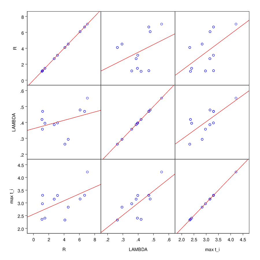
The correlation and the corresponding p-value of the t-test are reported in Table 6.1, wherecomputations have been done after putting apart the outlier corresponding to Brazil:

Correlation	$r$	$\lambda^{\star}$	$\max t_{i}$
$r$	$1$	$0.355589(0.2832)$	$0.553374(0.0774)$
$\lambda^{\star}$	$0.355589(0.2832)$	$1$	$0.725540(0.0115)$
$\max t_{i}$	$0.553374(0.0774)$	$0.725540(0.0115)$	$1$

This shows a significant positive relation between the maximal production process duration, and the growth rate, the relation is positive too with the spectral radius, but it not seem to be statistically significant.

7 Conclusion

This paper had a threefold purpose. First, we aimed at introducing a local measure of dominance based on the spectral properties of the input-output matrix. This has highlighted a local-global duality, in so far as the determinant is nothing more than the product of the eigenvalues.

Second, we wanted to reconcile sensitivity analysis and dominance theory - which was not possible without a local measure of dominance.

Third, we wished to give a new lecture of the input-output matrix in term of Markov chains, with a deeper interpretation of the underlying dynamics. One must of course bear in mind that the classical lecture is reduced to the analysis of mechanical transition, and does not enable one to determine the intrinsic and fundamental properties of the production process: interdependency and long run effects.

With respect to Lantner’s classification evoked at the beginning of our study, we thus place ourselves in the line of the first category of contributions, where we plan to bring further developments.

References

[Bre08] P. Bremaud. Markov chains: Gibbs fields, Monte Carlo simulation, and queues. Springer, 2008.
[DALW08] Y. Peres D. A. Levin and E. L. Wilmer. Markov chains and mixing times. American Mathematical Society, 2008.
[Die17] R. Diestel. Graph theory. Springer-Verlag, 2017.
[Fel68] W. Feller. An introduction to probability theory and its applications. Wiley, 1968.
[Har94] F. Harary. Graph theory. CRC Press, 1994.
[HEYZ15] F.-X. MEUNIER H. El Younsi, D. Lebert and C. ZYLA. Exploration, exploitation et cohérence technologique. Revue économie appliquée, 68(3), 2015.
[KS83] J. G. Kemeny and J. L. Snell. Finite Markov chains. Springer-Verlag, 1983.
[Lan72] R. Lantner. L’analyse de la dominance économique. Revue d’économie politique, 82(2):216–283, 1972.
[Lan15] R. Lantner. L’input-output est mort ? vive l’analyse structurale ! Revue économie appliquée, 68(3), 2015.
[LD01] M. Lahr and E. Dietzenbacher. Input-Output Analysis: Frontiers and Extensions. Palgrave Macmillan, 2001.
[Leb19] D. Lebert. Essais sur la théorie de la dominance économique, 2019.
[LL15] R. Lantner and D. Lebert. Dominance et amplification des influences dans les structures linéaires. Revue économie appliquée, 68(3):143–165, 2015.
[LY15] D. Lebert and H. El Younsi. Théorie de la dominance économique: indicateurs structuraux sur les relations interafricaines. Revue économie appliquée, 68(3), 2015.
[OCD18] OCDE. Stan input-output: Domestic output and imports. 2018.
[PO82] B. Peterson and M. Olinick. Leontief models, markov chains, substochastic matrices, and positive solutions of matrix equations. Mathematical Modelling, 3:221–239, 1982.
[Pon67] C. Ponsard. Les graphes de transfert et l’analyse économique des systèmes interrégionaux. Revue économique, 18(4):543–575, 1967.
[RAH13] C. R. Johnson R. A. Horn. Matrix Analysis. Cambridge University Press, 2013.